Neural networks in catchment hydrology: a comparative study of different algorithms in an ensemble of ungauged basins in Germany

This study presents a comparative analysis of different neural network models, including convolutional neural networks (CNN), long short-term memory (LSTM) and gated recurrent units (GRUs), with regard to predicting discharge within ungauged basins in Hesse, Germany. All models were trained on 54 catchments with 28 years of daily meteorological data, either including or excluding 11 static catchment attributes. The training process for each model scenario combination was repeated 100 times using a Latin hypercube sampler for hyperparameter optimisation with batch sizes of 256 and 2048. The evaluation was carried out using data from 35 additional catchments (6 years) to ensure predictions in basins that were not part of the training data. This evaluation assessed predictive accuracy and computational efficiency concerning varying batch sizes and input configurations and conducted a sensitivity analysis of dynamic input features. The findings indicated that all examined artificial neural networks demonstrated significant predictive capabilities, with a CNN model exhibiting slightly superior performance, closely followed by LSTM and GRU models. The integration of static features was found to improve performance across all models, highlighting the importance of feature selection. Furthermore, models utilising larger batch sizes displayed reduced performance. The analysis of computational efficiency revealed that a GRU model was 41 % faster than the CNN model and 59 % faster than the LSTM model. Despite a modest disparity in performance among the models (<3.9 %), the GRU model's advantageous computational speed rendered it an optimal compromise between predictive accuracy and computational demand.

1 Introduction

Artificial intelligence (AI) is increasingly being used to answer scientific questions, including those in the realm of hydrology (Kratzert et al., 2019a, b; Afzaal et al., 2019; Nabipour et al., 2020). The predictive accuracy of AI in these hydrological studies, particularly concerning discharge, is of paramount importance for flood control, watershed management or the estimation of water availability (Sharma and Machiwal, 2021; Brunner et al., 2021). In the era of climate change, which causes tremendous variability in rainfall patterns and increases evapotranspiration, the role of precise hydrological forecasts becomes even more essential (Tabari, 2020). An area of particular challenge is prediction in ungauged basins (PUB), an endeavour fraught with substantial uncertainty due to the lack of empirical data for model calibration (Blöschl, 2016). Effective models for PUB should thus possess robust generalisation capabilities across diverse watershed behaviours, enabling more universal basin type predictions (Sivapalan et al., 2003).

As demonstrated by Kratzert et al. (2019a), an artificial neural network (ANN) model, namely the long short-term memory (LSTM) network (Hochreiter and Schmidhuber, 1997), showed unprecedented accuracy in PUB. The employed LSTM model exhibited the ability to generalise rainfall–runoff predictions across a substantial number of basins (531), surpassing the performance of traditional hydrological models that typically operate best when independently calibrated for each separate basin. Further comparative analyses, such as those by Le et al. (2023), evaluated the performance of LSTM against other ANNs like multilayer perceptrons (MLPs) and convolutional neural networks (CNNs) in daily streamflow prediction. This study revealed superior performance by LSTM and CNN models over conventional ANNs, with LSTM exhibiting a marginal edge over CNN. Moreover, a novel approach proposed by Ghimire et al. (2021) involved a hybrid CNN–LSTM model, designed for hourly discharge predictions. When benchmarked against various ANNs (CNN; LSTM; deep neural network – DNN), traditional AI models (extreme learning machine, MLP) and ensemble methods (decision tree, gradient boosting regression, extreme gradient boosting, multivariate adaptive regression splines), the CNN–LSTM model displayed superior performance with regard to multiple evaluation metrics, although all ANNs exhibited high efficacy. This is evidence that deep learning, a subset of machine learning characterised by multilayered ANNs, holds substantial promise for streamflow prediction. However, while numerous studies have explored discharge prediction using ANNs, only a limited number have conducted comparative analyses of different ANN architectures. Table 1 summarises these studies from 2020 to December 2023, noting that most incorporate lagged target variables as inputs. This methodology, though effective, is less applicable for PUB due to the absence of discharge data in ungauged or poorly gauged regions, necessitating the use of discharge-independent inputs.

Among the studies shown in Table 1, three specifically addressed this constraint. The first, by Nguyen et al. (2023a), evaluated CNN and LSTM models for daily discharge prediction in the 3S river basin, exclusively using daily mean temperature and precipitation data. This study adopted a “regional” approach, akin to that of Kratzert et al. (2019a), training both model architectures with data from all three sub-basins. The LSTM was found to outperform the CNN, although the latter's results were not extensively discussed. The second study, by Wegayehu and Muluneh (2023), contrasted three super ensemble learners against eight base models, including LSTM, a gated recurrent unit model (GRU) and a compound CNN–GRU model, for daily discharge prediction. Here, the LSTM ranked among the top three in four out of five scenarios based on R² metrics. However, its performance declined significantly in the absence of feature selection, indicating susceptibility to redundant features. Notably, this study trained separate models for each basin, thus not directly addressing PUB generalisation capabilities. The third study, by Oliveira et al. (2023), compared three ANN models (LSTM, CNN and MLP) for daily discharge estimation in a single basin, where the CNN model exhibited superior performance (Nash–Sutcliffe efficiency (NSE) of 0.86). However, this does not imply generalisability in non-calibrated catchments as both calibration and testing occurred within the same basin. Regrettably, this limitation pertains to all three studies. Consequently, this research aimed to bridge the existing literature gap by comparing the performance of three distinct ANN architectures for predicting discharge in ungauged basins. Through a comparative analysis, this study not only addresses a significant gap in hydrological literature but also provides valuable insights into the relative strengths and limitations of each ANN model, thereby guiding future applications and development in the field of hydrological prediction. Furthermore, a comprehensive sensitivity analysis was conducted to identify key drivers affecting the prediction of each model. This methodological approach contributes to refining model selection and calibration strategies in hydrological forecasting.

The first architecture under examination was the LSTM, which demonstrated robust performance in numerous studies (Kratzert et al., 2019a, b; Le et al., 2023; Nguyen et al., 2023a). Although LSTM models demonstrated promising performance, the inherent sequential architecture of LSTM led to higher computational costs. This resulted in a relative decrease in computational efficiency when compared to feed-forward neural networks or CNNs, as discussed in Gauch et al. (2021). In pursuit of addressing these limitations and challenges that are inherent to LSTM models, the second architecture chosen for examination was the CNN. This model is characterised by its parallel processing capabilities, significantly boosting computational efficiency, a critical factor when handling large-scale, high-resolution time series data; extensive input sequences; and a multitude of input features (Bai et al., 2018). The third architecture under consideration was the gated recurrent unit. GRU, a variant of LSTM, is recognised for its proficiency in effectively capturing temporal dependencies in time series data while imposing less computational burden (Cho et al., 2014).

Given that PUB is often characterised by data scarcity, this study incorporated two distinct scenarios: the first involving the use of only daily forcing data and the second extending this with additional static catchment features. This approach allowed for an evaluation of the model's generalisation capacity when constrained to minimal data. Additionally, it provided insights into the degree to which static catchment features could contribute to enhancing model performance, as indicated by Kratzert et al. (2019a). Accordingly, the objectives of this study were delineated as follows:

1. to evaluate the potential of predicting discharge in ungauged basins by means of daily forcing data with ANNs, namely LSTM, CNN and GRU;

2. to compare the computational efficiency of LSTM, CNN and GRU models for daily time series prediction;

3. to investigate the potential of static features to enhance prediction performance; and

4. to assess the impact of batch size on model performance and computational efficiency.

Nguyen et al. (2023a)Wegayehu and Muluneh (2023)Oliveira et al. (2023)Nguyen et al. (2023b)Cheng et al. (2020)Vatanchi et al. (2023)Le et al. (2023)Haznedar et al. (2023)Hong et al. (2020)Le et al. (2021)Li et al. (2022)Hong et al. (2021)Deng et al. (2022)Herbert et al. (2021)

Table 1 Overview of recent studies focused on comparing discharge prediction using various artificial neural networks. “Target independence” indicates that discharge data were not utilised as input features during model training and/or testing. “Ungauged” indicates model evaluation with catchments that were not part of the training dataset. “Multi-catchment” denotes that the models were evaluated on multiple catchments.

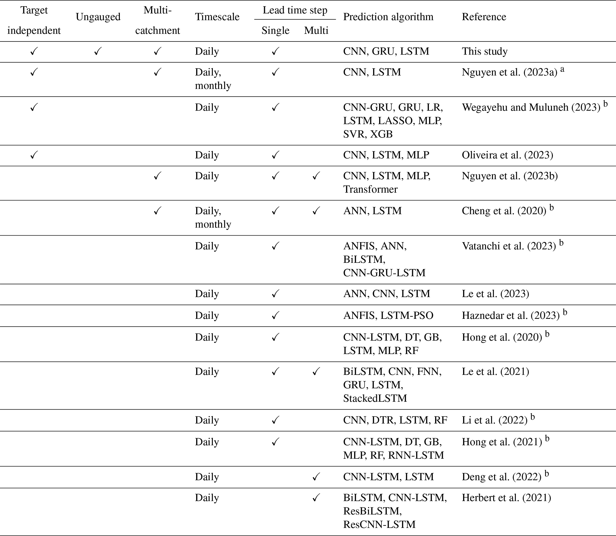
ANFIS denotes adaptive neuro-fuzzy inference system, ANN denotes artificial neural network, BiLSTM denotes bidirectional LSTM, CNN denotes convolutional neural network, DT denotes decision tree, DTR denotes decision tree regressor, FNN denotes feed-forward neural network, GB denotes gradient boosting, GRU denotes gated recurrent unit, LSTM denotes long short-term memory, LR denotes linear regression, MLP denotes multilayer perceptron, LASSO denotes least absolute shrinkage and selection operator, PSO denotes particle swarm optimisation, Res denotes residual, RF denotes random forest, RNN denotes recurrent neural network, SVR denotes support vector regression, and XGB denotes extreme gradient boosting. ^a Only the results of the LSTM model are stated. ^b Hyperparameter configuration nontransparent.

2 Materials and methods

2.1 Study area

All basins analysed in this study are located in the federal state of Hesse, Germany (Fig. 1). The climate of this region is temperate–humid and is characterised by moderate temperature and precipitation levels (Heitkamp et al., 2020). The topography of Hesse, characterised by a complex blend of lowlands, hilly terrains and modest mountain ranges, fosters a multifaceted hydrological setting. A variety of geological formations and soil types within the region contribute to the mixed pattern of infiltration rates, groundwater recharge and surface runoff (Jehn et al., 2021).

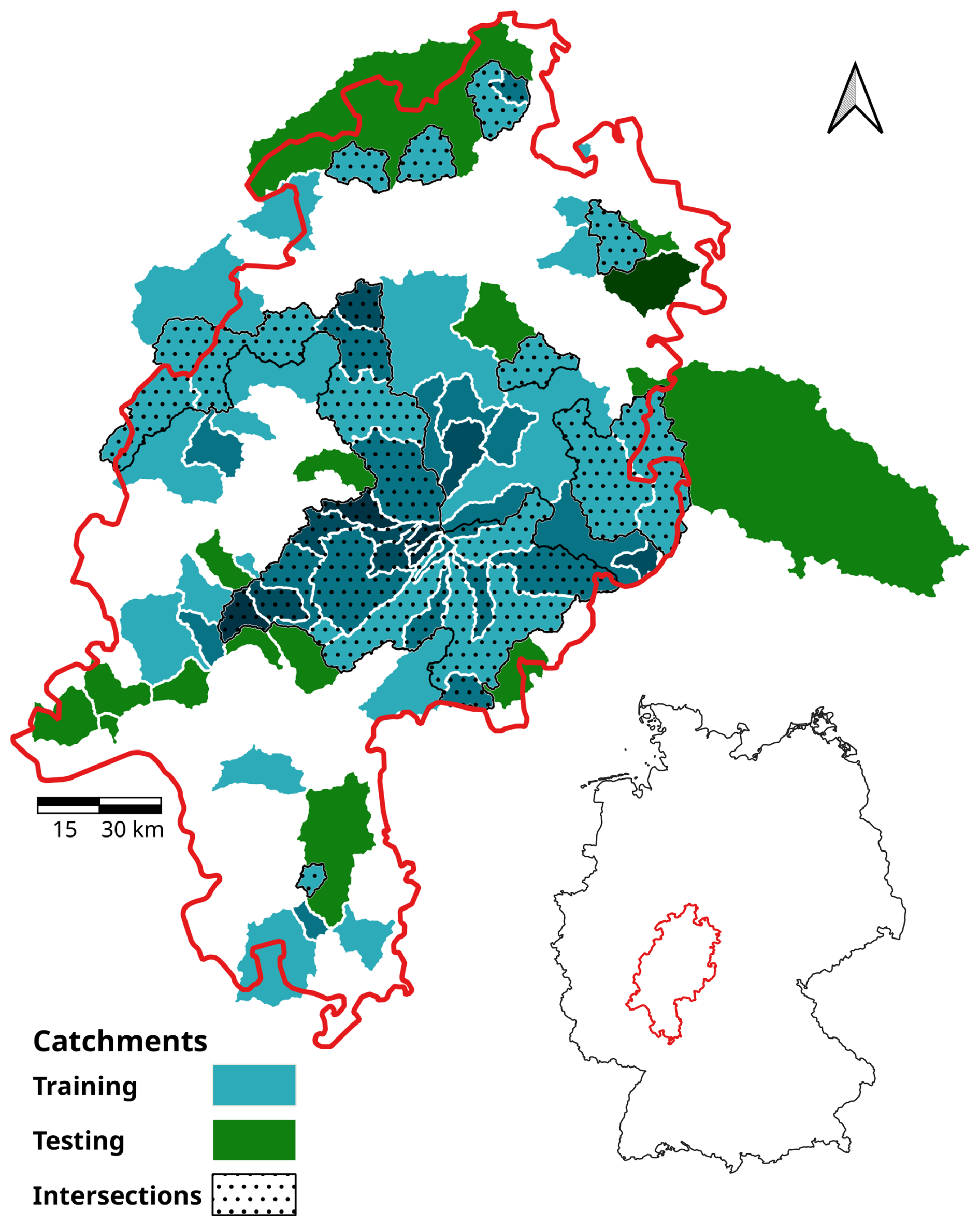
Figure 1 Geographic distribution of the catchments in Hesse and Hesse's location within Germany. Darker shades represent nested catchments, while intersections indicate catchments partially incorporated into both training and testing phases.

2.2 Data sources

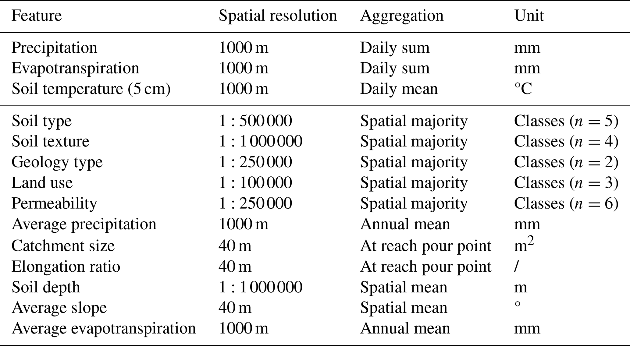
The dataset used in this study was derived from Jehn et al. (2021). For each catchment, daily sums of precipitation [mm], daily sums of evapotranspiration [mm] and soil temperature at 5 cm soil depth [°C] were available along with the corresponding discharge [mm]. The discharge data were obtained from a gauging station located within the respective catchment. In addition, the dataset included 11 static catchment features corresponding to every catchment (Table 2). As suggested by Kratzert et al. (2019a), the inclusion of static catchment attributes can improve the performance of machine learning models. Table 2 provides an understanding of the underlying aggregation of data, spatial resolution and units. Apart from discharge data, which are accessible upon contacting the Hessian Agency for Nature Conservation, Environment and Geology, all other datasets are publicly available within the associated repository of Jehn (2020).

Table 2 Summary of daily forcing data and static catchment attributes utilised for modelling: detailing the spatial resolution of the original data sources with the aggregation methods and the respective units.

2.3 Data preprocessing

The preprocessing of the input data was an essential step to ensure that the quality and integrity of the data were maintained. This process entailed a detailed analysis of data continuity, encoding of non-numerical values, and splitting of the dataset into training and validation subsets, followed by data normalisation and subsequent transformation. The data analysis revealed discontinuities in the discharge data across the time series of 39 catchments. In order to provide the longest possible time series for the training process, a total of 54 out of the full set of 95 catchments were selected for model training. These catchments covered 28 years (1991–2018). Of the remaining 39 catchments, 35 were utilised for testing, each with a temporal resolution spanning 6 years from 1997 to 2002. Rivers containing artificial constructions that impede discharge through impoundments (e.g. reservoirs) were not considered in this analysis. However, it should be noted that a subset of the selected rivers might be equipped with hydraulic control mechanisms, such as floodgates (Jehn et al., 2021).

For both training and testing datasets, all categorical features (Table 2) were encoded using label encoding. In this approach, every unique variable of a categorical feature was replaced by a non-repeatable integer value (Lin et al., 2020). This method was preferred over the frequently recommended one-hot-encoding technique (Duan, 2019; Cerda and Varoquaux, 2022) in order to circumvent an increase in the total feature count equivalent to the number of unique feature variables, as occurs with the one-hot-encoding technique (Ul Haq et al., 2019). Moreover, label encoding accommodates ordinal scales, which are better suited for hierarchical features such as permeability. In contrast, categorical features without a meaningful order, such as soil type or soil texture, are better handled by the one-hot-encoding technique, which treats each category independently. Furthermore, Potdar et al. (2017) indicated that label encoding yielded the lowest performance among various investigated encoding methods. Consequently, it cannot be unequivocally asserted that this method stood as the optimal approach. To avoid further increasing the number of static input features, label encoding was selected.

The training dataset of 54 catchments was then further divided, using 80 % of the data for training and 20 % for validation. Subsequently, the two datasets were normalised by employing a min–max scaling method, with a range of [0,1] chosen as the boundaries. The choice of this scaling method was made empirically based on the observed performance in the dataset and model configuration. Concurrently, the precision of the data representation was configured to adhere to a float32 format. The target variable was scaled independently of the features. Moreover, to prevent data leakage, each feature normalisation was established solely based on the training dataset.

The normalised training dataset exhibited a shape of N×D for each catchment, where N signified the number of samples in time, and D represented the number of features. To assess the impact of additional static features, two distinct datasets were created. The first dataset included only three features with daily forcing data and assumed a shape of N×3, while the second incorporated all 11 static features and took a shape of N×14.

To transform the datasets into training batches, a two-dimensional moving window, characterised by dimensions of T×D, was subsequently implemented, where T represents the moving-window size, also known as the look-back period or sequence length (Fig. 2). This window is continuously incremented by a single period in the dimension of N, with the initial window encompassing observations [N₁, N_T]. The consecutive window encapsulates observations $[N_{\mathrm{2}},N_{T+\mathrm{1}}]$, and this pattern is maintained until the window reaches the final element of the dataset (N_n). Consequently, the entire dataset was partitioned into $m=N_{n-T+\mathrm{1}}$ subsamples for every catchment. All subsamples were combined into a three-dimensional array ($N_{n-T+\mathrm{1}}\times T\times D$). The transformed catchment datasets were stacked into one final training set with the shape of $C\times N_{n-T+\mathrm{1}}\times T\times D$, where C was equal to the number of catchments. The identical transformation was implemented for both validation and test datasets, encompassing those with and without static features.

It is important to note that the transformation of the data is already part of the hyperparameterisation process, a concept further elucidated below.

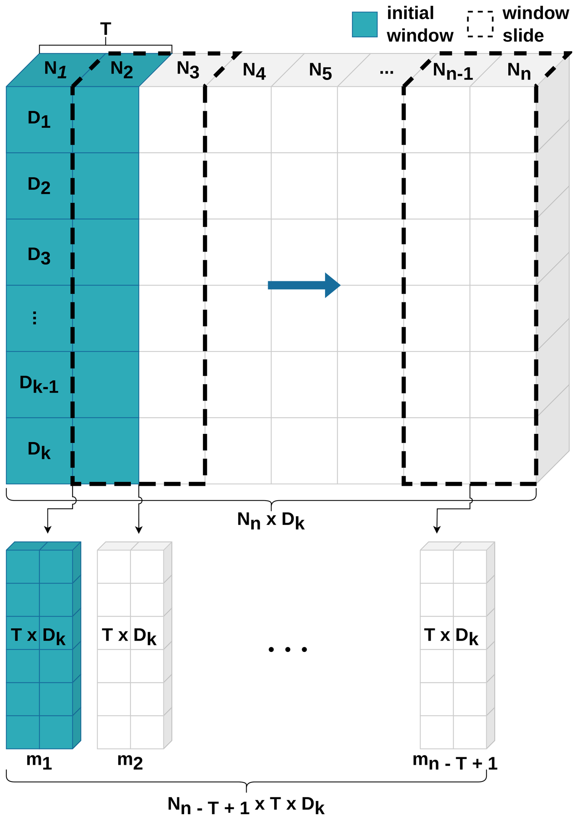
Figure 2 Schematic procedure of data transformation by applying a moving window: this procedure primarily involves the partitioning of the data into distinct sections, employing a window (blue) that slides across the dataset, effectively creating a temporal snapshot (m). T delineates the window size within the temporal dimension, D represents the feature dimension, and N signifies the temporal samples with a daily resolution.

2.4 Hyperparameterisation

The performance of machine learning models is influenced by the optimisation of their respective hyperparameters (Shekhar et al., 2022; Ozaki et al., 2021). In the domain of machine learning, hyperparameters are variables that define the configuration of the models and are set prior to the training process (Bhattacharjee et al., 2021), while the term parameter refers to the variables that the model learns during training (Goodfellow et al., 2016). The selection of an appropriate tool for hyperparameter optimisation is a critical step. Consequently, this task was conducted utilising a Python framework known as Spotpy (Houska et al., 2015). The framework offers computational optimisation techniques for calibrating models, such as a Latin hypercube sampler (LHS), an appropriate method for selecting input variable values within a specified range given its ability to generate near-random samples from a multidimensional hyperparameter distribution (McKay et al., 1979).

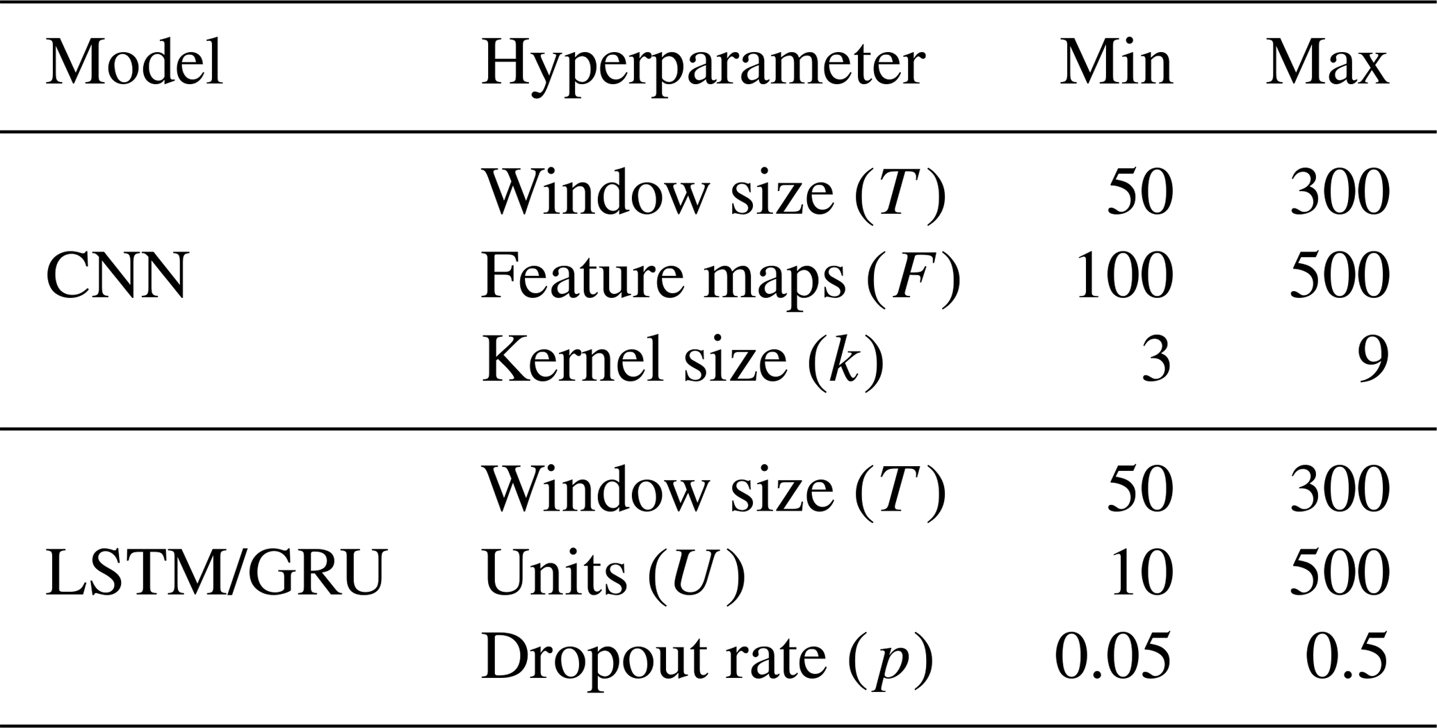
The hyperparameters of the models are contingent upon the architectural design. In this study, three distinct model architectures were explored: LSTM, GRU and CNN. LSTM and GRU are both types of recurrent neural networks (RNNs), specifically designed to handle sequential data, such as time series. As the employed LSTM and GRU models possess an identical layer structure, both models share an equivalent set of hyperparameters. A detailed overview of the utilised hyperparameters can be found in Table 3.

The hyperparameter T denotes the window size employed in the moving-window mechanism and signifies the length of the sequence, representing how many time steps (past days) are used to predict the discharge of the following day. The feature maps F quantify the number of results or features generated within the convolution process. This is achieved by utilising a kernel of size k, referred to as the filter size, which is systematically applied over the data to extract essential patterns and characteristics, thereby transforming the input data.

In the context of LSTM and GRU models, the unit U refers to the number of hidden neurons within the RNN layer. This quantity not only characterises the internal complexity of the layer but also corresponds to the output dimension. The final hyperparameter under consideration is the dropout rate p, which represents the fraction of the neurons that are randomly set to zero during training (Srivastava et al., 2014).

The ranges of the hyperparameters were delineated in preliminary experiments by repeatedly training each model employing LHS over wider ranges. Any hyperparameter that fell below or exceeded the minimum and maximum bounds of Table 3 demonstrated inferior performance on average. The final training process was executed with a sampling size of 100 for each model and batch size combination, with and without static features. This culminated in a total of 12 distinct sampling processes.

Table 3 Ranges of hyperparameters deployed across different neural network models within the Latin hypercube sampling framework.

2.5 Model architectures

The architecture of the LSTM was first introduced by Hochreiter and Schmidhuber (1997). An LSTM consists of a memory cell governed by four specific gate units, granting the capacity to preserve information over extended periods (Cho et al., 2014). Through this architectural design, LSTMs possess the capability to mitigate the challenges associated with exploding or vanishing gradients, as encountered in traditional RNNs. While the nuanced workings of LSTM cells and their concomitant advantages are pertinent (Hochreiter and Schmidhuber, 1997), they have been extensively discussed in prior research and thus will not be repeated within this study.

The architectural design of a GRU model is inspired by the structure of LSTMs, with the distinction that it incorporates only two gates to regulate the information flow. This results in reduced computational complexity, thereby rendering GRUs more computationally efficient while still addressing the exploding- and vanishing-gradient problem (Cho et al., 2014).

In contrast, CNNs are tailored for grid-like data structures, including images. The CNN architecture was first introduced by Fukushima (1980). The term convolutional neural network was introduced by LeCun et al. (1989), who developed a model for handwritten digit recognition.

CNN models possess a significant advantage in that the convolution operation is inherently parallelisable, allowing for the simultaneous execution of numerous calculations. An additional merit is the ability to extract features irrespective of the exact location where the feature is found. This reduces the number of input samples needed for training and thus improves computational efficiency (Lecun et al., 1998). Note that these extracted features are distinct from those listed in Table 2.

The architectural configurations of the three models employed in this study are depicted in Fig. 3, with further explanations provided in the subsequent sections.

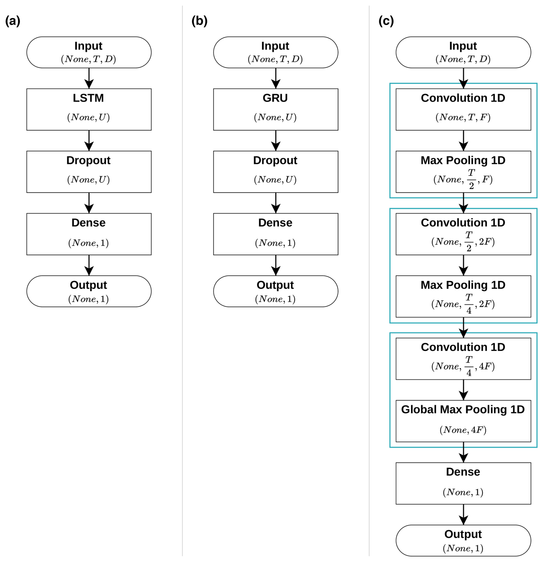
Figure 3 Schematic diagrams of the architectures of the three utilised models: (a) long short-term memory (LSTM), (b) gated recurrent unit (GRU) and (c) convolutional neural network (CNN).

2.5.1 LSTM

The LSTM model comprises a single LSTM layer configured with a designated number of hidden units (U). To mitigate overfitting and promote generalisation, a dropout layer is directly connected to the LSTM layer, introducing regularisation by randomly deactivating a specific fraction (dropout rate) of the hidden units (Srivastava et al., 2014).

The final layer is a dense layer that applies a sigmoid activation function, which converts the output into a probability value between 0 and 1 (Fig. 4c). The adoption of this specific activation function was motivated by the need to prevent the generation of negative discharge predictions, which were previously encountered with the use of alternative activation functions like LeakyReLU or a linear function. Such negative predictions are hydrologically implausible and undermine the validity of the model outputs. However, the utilisation of a sigmoid function, in conjunction with a min–max scaling technique, introduces a structural limitation wherein the model is incapable of extrapolating beyond the maximum discharge values observed during the training phase. Considering these trade-offs, the sigmoid function was chosen as a compromise to balance model stability and physical realism.

A comprehensive examination of all activation functions employed within the models is provided in Fig. 4. This illustration delineates the specific characteristics of each function, highlighting that both the rectified linear unit (ReLU) and sigmoid functions are designed to avoid negative values. The ReLU function, in particular, suppresses negative values by setting them to 0, while the sigmoid function, recognised by its characteristic S shape, maps any input into values between 0 and 1. Pertinently, in the context of deep learning, especially in image recognition, ReLU is often favoured for its expedited learning capabilities, yielding enhanced performance and superior generalisation attributes (Krizhevsky et al., 2017). However, it was observed in preliminary experimental setups that the sigmoid function exhibits greater stability, while ReLU demonstrated a higher propensity to induce gradient exploding. The complete architectural design of the LSTM model is illustrated in Fig. 3a.

2.5.2 GRU

The architecture of the GRU model shares a structure similar to that of the previously described LSTM model, with the primary difference being the substitution of the LSTM layer with a GRU layer (Fig. 3b). Similarly to the LSTM model, the GRU model contains a single layer configured with a designated number of hidden units (U) and employs a dropout layer directly connected to the GRU layer to mitigate overfitting and to promote generalisation. The final dense layer similarly employs a sigmoid activation function to ensure that all predicted discharge values remain within a physically plausible range.

2.5.3 CNN

The CNN is composed of a series of three convolution cells, each containing a one-dimensional convolution layer followed by a pooling layer. The convolution layers incorporate a ReLU activation function (Fig. 4b) and employ a sliding-window mechanism known as a kernel that traverses the input data for processing. As previously elucidated, this kernel is responsible for extracting feature maps (F) from time-dependent input features. The kernel, with a size of k, is applied uniformly across all convolution layers. In each successive convolution layer, the quantity of feature maps is increased by a factor of 2, thereby enhancing the model's capacity to extract and represent complex features.

In the initial pair of convolution cells, the temporal dimension (T array) within the pooling layer is reduced by a factor of 2 by employing a stride of size 2 across each T array, while the third pooling layer extracts a single set of feature maps along the temporal axis of all T arrays. To preserve the temporal dimension during the convolution process, each convolution layer incorporates symmetric zero-padding. This technique involves adding zeros around the input data, ensuring that the processed dimension remains unchanged after applying the convolution operation.

The last layer of the model is a dense layer that compresses the model dimensions to produce a single output value for each prediction. This layer is fully connected to the preceding layer and uses a leaky rectified linear unit (LeakyReLU) activation function as depicted in Fig. 4b. The LeakyReLU, akin to the standard ReLU (shown in the same figure), differs by introducing a small, non-zero slope for negative values. This characteristic enhances gradient propagation and mitigates the issue of vanishing gradients (Ramachandran et al., 2021).

The selection of the LeakyReLU over the standard linear activation function (Fig. 4a) was driven by the latter's propensity to generate negative predictions for the discharge values. Although LeakyReLU does not entirely preclude negative predictions, it effectively modulates them into marginally negative outputs and therefore reduces the extent of negative predictions. Although the sigmoid function is effectively utilised in LSTM and GRU models to prevent negative discharge predictions, its application within the CNN model framework yielded suboptimal results in preliminary trials, particularly when compared to the performance achieved using the LeakyReLU activation function. This informed the decision to opt for LeakyReLU in our work.

A visual representation of the complete architectural design of the CNN model is presented in Fig. 3c.

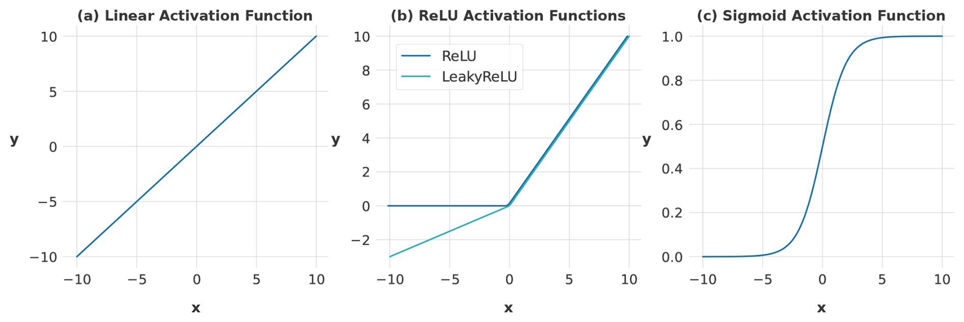
Figure 4 Visualisation of the three activation functions utilised within the employed models. The diagrams show the graphical representations and functional ranges of (a) the linear function, which preserves the raw, untransformed input; (b) the rectified linear unit (ReLU) function, which maps negative inputs to zero and passes positive inputs unchanged; and (c) the sigmoid function, characterised by its distinct S shape, which compresses any input into a range between 0 and 1. Note the different y-axis scales.

2.6 Loss function

In machine learning algorithms, the role of the loss function is paramount as it quantifies the discrepancy between the model's predictions and the actual data (Wang et al., 2022). The optimiser, an algorithm designed to minimise the loss, regulates the process of updating the model's parameters. This optimiser strives to enhance model performance by iteratively determining the loss and then adjusting the model parameters to reduce this loss. This is achieved by identifying the gradient or derivative of the loss function, which denotes the local minimum (least steep ascent). Thus, by minimising the loss, the machine learning model can improve its predictive accuracy.

The optimiser used for all models in this study is the Adam optimiser (Kingma and Ba, 2017). This algorithm provides high computational efficiency for gradient-based optimisation and is suitable for large models that include a high number of parameter sets.

The choice of loss function is dictated by the specific task at hand. A commonly used loss function when predicting continuous data is the mean square error (MSE), which is favoured for its computational efficiency. However, MSE suffers from sensitivity to outliers due to its quadratic penalty and exhibits scale dependence, rendering it less interpretable and comparably challenging when evaluating models across disparate output scales (Liano, 1996; Gupta et al., 2009).

Another metric used to capture model performance, traditionally employed in hydrology, is the Nash–Sutcliffe efficiency (NSE) (Knoben et al., 2019). Based on the close similarities between MSE and NSE and, hence, the inherent disadvantages, NSE is not an ideal choice as a loss function either (Gupta et al., 2009).

To mitigate the systematic issues encountered in optimisation processes that arise from formulations linked to the MSE or NSE, we decided to utilise the more resilient Kling–Gupta efficiency (KGE). KGE corrects for underestimation of variability by providing a direct evaluation of four different facets of the discharge time series, encompassing shape, timing, water balance and variability (Santos et al., 2018). The definition of KGE is delineated in Eq. (1):

$$\begin{array}{}\text{(1)}& \text{KGE}=\mathrm{1}-\sqrt{{\left(r-\mathrm{1}\right)}^{\mathrm{2}}+{\left(\mathit{\alpha }-\mathrm{1}\right)}^{\mathrm{2}}+{\left(\mathit{\beta }-\mathrm{1}\right)}^{\mathrm{2}}},\end{array}$$

with

$$\begin{array}{rl}& r={\displaystyle \frac{{\text{Cov}}_{\left(\text{obs, sim}\right)}}{{\mathit{\sigma }}_{\text{obs}}\cdot {\mathit{\sigma }}_{\text{sim}}}},\\ & \mathit{\alpha }={\displaystyle \frac{{\mathit{\sigma }}_{\text{sim}}}{{\mathit{\sigma }}_{\text{obs}}}},\\ & \mathit{\beta }={\displaystyle \frac{{\mathit{\mu }}_{\text{sim}}}{{\mathit{\mu }}_{\text{obs}}}},\end{array}$$

where μ is the mean, σ is the standard deviation, and r is the linear correlation factor between observations and simulations. The variable α is a measure of how well the model captures the variability of the observed data, and β defines a bias term indicating how much the model's predictions systematically deviate from the true values (Knoben et al., 2019).

Analogously to NSE, KGE also indicates the highest performance when equal to 1. However, the goal of the loss function is to minimise the error; thus, the discrepancy between simulation and observation should approach 0. Therefore, the implemented loss function L results in Eq. (2).

$$\begin{array}{}\text{(2)}& L_{\left(\text{obs, sim}\right)}=\sqrt{{\left(r-\mathrm{1}\right)}^{\mathrm{2}}+{\left({\displaystyle \frac{{\mathit{\sigma }}_{\text{sim}}}{{\mathit{\sigma }}_{\text{obs}}}}-\mathrm{1}\right)}^{\mathrm{2}}+{\left({\displaystyle \frac{{\mathit{\mu }}_{\text{sim}}}{{\mathit{\mu }}_{\text{obs}}}}-\mathrm{1}\right)}^{\mathrm{2}}}\end{array}$$

2.7 Model training

The training process was conducted using a GeForce RTX 3090 graphics card equipped with 24 GB of memory. Each model was subjected to training with batch sizes of 256 and 2048. The batch size is a fraction of the total number of training samples and represents the number of samples utilised to train the model prior to an update of the internal parameters (Radiuk, 2017).

The batch size has no physical interpretation in the context of hydrological processes but functions as a crucial hyperparameter in the training of neural networks. Prior studies, such as that of Kratzert et al. (2019a, b), have demonstrated the successful application of a batch size of 256. In this study, this batch size was also adopted and served as the baseline. To further explore the impact of larger batch sizes, a multiple of 256 was employed. A batch size of 2048 was then utilised, representing the upper limit of the memory capacity of the graphics card used.

The maximum number of epochs designated for training was set to 60. An epoch refers to a single iteration over the entire training dataset during which the model's parameters are adjusted to minimise loss. However, the training process was configured to terminate when the validation loss failed to show improvement throughout five consecutive epochs. An enhancement was recognised when the validation loss decreased by a minimum of 0.001 during these five epochs. This mechanism is called early stopping.

Given that the input data for the training procedure are arranged by catchments, shuffling of data was implemented to circumvent the potential for overfitting to a specific catchment. Furthermore, each model was trained both with and without the inclusion of static features for the two specified batch sizes. This leads to a total of four distinct training phases for every model with a specific hyperparameter set.

The static features were processed analogously within the models in relation to the treatment of the daily features. The learning rate, frequently acknowledged as the paramount hyperparameter to tune, exerts a considerable influence on the training of models that employ gradient descent algorithms (Xu et al., 2019).

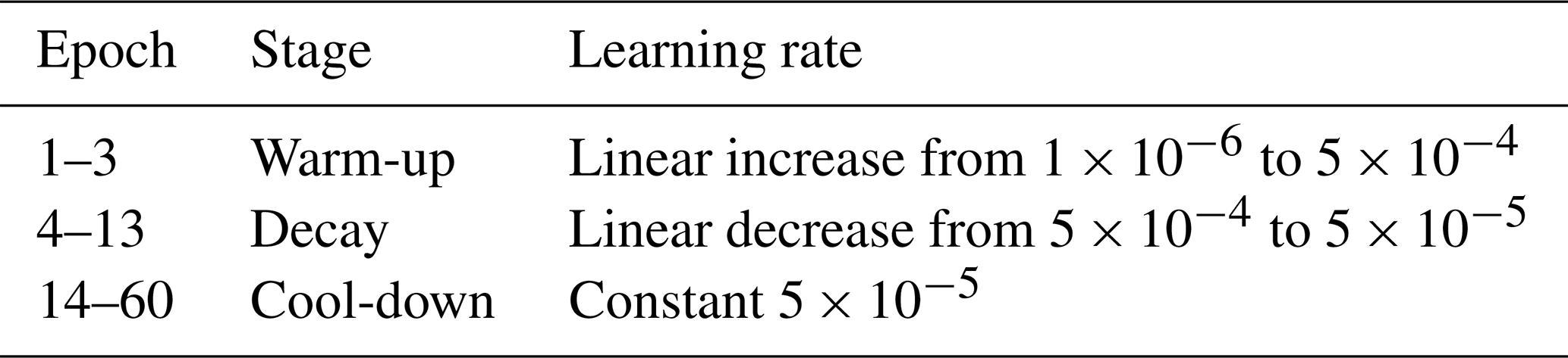
When the learning rate is too high, the optimiser may diverge from the local minimum, while setting it too low can result in a protracted learning process (Zeiler, 2012). To efficiently address this behaviour, a dynamic adjustment of the learning rate was integrated into the training process using a learning-rate scheduler.

This algorithm modifies the learning rate based on the current epoch number. During the warm-up period, the learning rate linearly increased from the initial rate to the base rate throughout three epochs. The warm-up period was followed by a decay period lasting 10 epochs, during which the learning rate linearly decreased from the base rate to the minimum rate. Following the decay phase, the learning rate was kept constant at the minimum rate for the remaining epochs. Detailed information can be found in Table 4.

Table 4 Gradual alterations in the learning rate throughout the 60 epochs of the model training process.

3 Results and discussion

3.1 Model performance

The analysis depicted in Fig. 5 delineates a comparative evaluation of model performance concerning architectural variations, batch sizing and the incorporation of supplementary static attributes. The findings reveal that employing CNN models in conjunction with static features yielded a mean KGE of 0.80 and 0.78 for batch sizes of 256 and 2048, respectively. The inclusion of static features provides a performance benefit as the mean accuracy drops to 0.71 and 0.67 when static features are omitted for batch sizes of 256 and 2048, respectively. This aligns with the findings presented by Kratzert et al. (2019b), who assert that static catchment attributes enhance overall model performance by improving the distinction between different catchment-specific rainfall–runoff behaviours.

Notably, the maximum KGE in the absence of static features reached 0.97 and 0.92 for batch sizes of 256 and 2048, respectively, highlighting the potential for high model performances even without static features. On the contrary, the minimum KGE drops when omitting static features to −0.21 and −0.26 for batch sizes of 256 and 2048, respectively, showing the lowest minimum performance of all models. This suggests a deficiency in the model's ability to generalise, a phenomenon frequently observed when overfitting occurs (Srivastava et al., 2014).

Regarding the minimum KGE values when utilising static features, the CNN models demonstrated the third and fourth highest minimum values, registering at 0.24 and 0.20 for batch sizes of 256 and 2048, respectively.

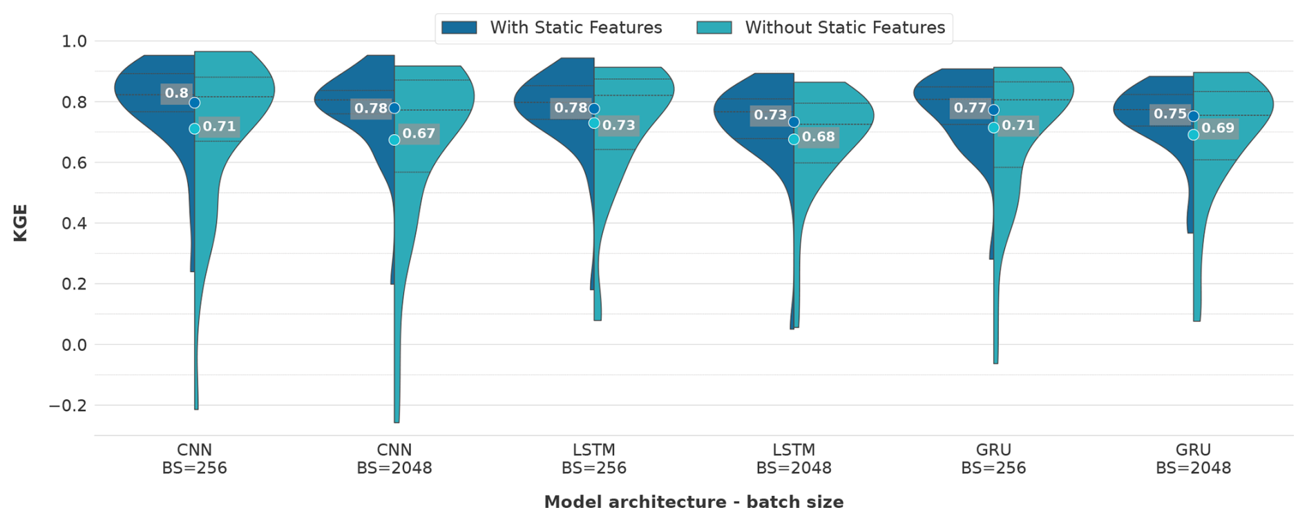
Figure 5 Evaluation of performance discrepancies in the applied models relative to batch size and additional static catchment attributes during the testing period. The number represents the average KGE over all 35 catchments. The dotted line displays the percentile intervals.

In the case of LSTM networks, mean KGE values of 0.78 and 0.73 with static features for batch sizes of 256 and 2048, respectively, can be noted. The mean KGE declined to 0.73 and 0.68 when static features were omitted for batch sizes of 256 and 2048, respectively. Notable is the maximum performance achieved with static features, which reached 0.94 for a batch size of 256. In contrast, the LSTM with a batch size of 2048 exhibited the lowest minimum value of 0.05 across all models with static features. For models run without static features, the LSTM with a batch size of 256 recorded the highest minimum value of 0.09. Conversely, the LSTM model with no static features and a batch size of 2048 presented the lowest maximum KGE of 0.86.

For GRU, the mean KGE exhibited similar trends with the inclusion of static features, reaching 0.77 and 0.75 for batch sizes of 256 and 2048, respectively. The mean performance declined to 0.71 and 0.69 when static features were omitted for batch sizes of 256 and 2048, respectively. The GRU model with a batch size of 2048 demonstrated the highest minimum KGE value of 0.37 among all models when static features were incorporated. Following closely, the GRU model with a batch size of 256 under the same feature scenario presented the second highest minimum KGE of 0.28.

Upon examining the performance range, the GRU model with static features and a batch size of 2048 exhibited the narrowest performance range of 0.52. Subsequently, the GRU model with static features and a batch size of 256 displayed a performance range of 0.63, indicating robust generalisation capabilities for these two models. Notably, for both batch sizes, the GRU model demonstrated a marginally higher maximum KGE when static features were omitted. This finding contradicts the outcomes of all other models, where the inclusion of static features consistently reduced the maximum KGE, regardless of batch size. The sole exception to this pattern was observed in the CNN model with a batch size of 256 and utilising no static features.

Altogether, when analysing the influence of batch size across various models, it becomes evident that an increase in batch size correlates with a decrease in performance. This observation is confirmed by the study of Masters and Luschi (2018), who discovered that smaller batch sizes contribute to enhanced training stability and generalisation performance when employing CNN models for image classification. Additionally, Kandel and Castelli (2020) identified a strong correlation between learning rate and batch size, proposing that higher learning rates should be employed when utilising larger batch sizes. However, the learning rate remained constant across varying batch sizes throughout this study.

Altogether, these results suggest the following:

1. The smaller batch size of 256 contributes to better model performance with regard to mean KGE values.

2. Static features generally improved the mean KGE across all architectures and batch sizes.

3. The CNN model with static features and a batch size of 256 showed the highest mean KGE and therefore outperforms LSTM and GRU models slightly.

4. The KGE performance ranges for models with static features are substantially smaller and at a higher level than the ranges for models without static features.

5. Overall, the GRU model with a batch size of 256 and static features exhibited favourable KGE performances akin to LSTM and CNN models and mitigated poor predictions across all test catchments.

Comparing evaluation metrics

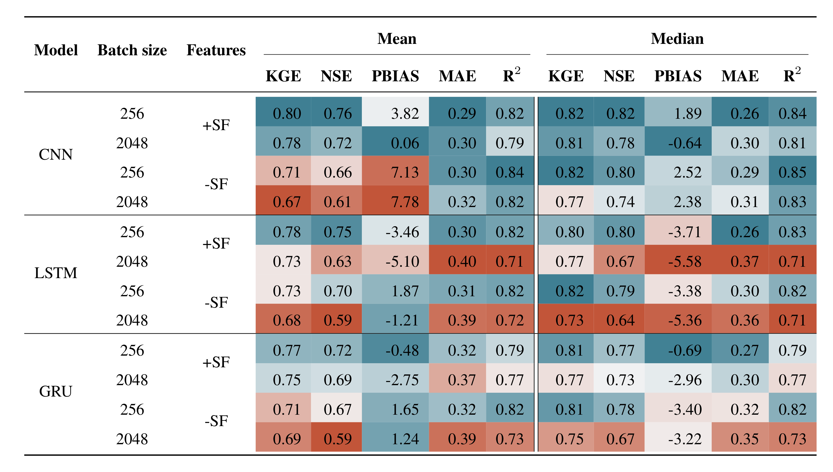
To further investigate the efficacy of the applied models, additional performance metrics were incorporated. Among these, the NSE was selected to facilitate comparison with prior studies that conventionally utilise this metric. Moreover, the percent bias (PBIAS) was employed to gauge the systematic deviation of the modelled data from observed values, indicating whether the model predictions consistently overestimate or underestimate the observations (Moriasi et al., 2007). The mean absolute error (MAE) was integrated as a metric to quantify the absolute discrepancies between model predictions and actual observations, serving as a direct assessment of model precision (Siqueira et al., 2016). Lastly, the coefficient of determination (R²) was adopted as an indicator for evaluating the degree of alignment between simulations and observed data, reflecting the model's “goodness of fit” (Onyutha, 2022). A comparative view of the results of all of the employed performance metrics is shown in Table 5.

Overall, the presented data indicate that NSE metrics are marginally lower than the KGE values. This phenomenon could potentially stem from the presence of counterbalancing errors, an inherent limitation associated with the KGE metric. Such counterbalancing errors materialise through concurrent overestimation and underestimation of the predictive target. Given that bias and variability collectively constitute two-thirds of the KGE, their effects may augment the aggregate score without necessarily indicating a more accurate or relevant model (Cinkus et al., 2023).

$$\begin{array}{}\text{(3)}& {\displaystyle }\text{NSE}=\mathrm{1}-{\displaystyle \frac{{\sum }_{i=\mathrm{1}}^N({\text{obs}}_i-{\text{sim}}_i{)}^{\mathrm{2}}}{{\sum }_{i=\mathrm{1}}^N({\text{obs}}_i-\stackrel{\mathrm{‾}}{\text{obs}}{)}^{\mathrm{2}}}}\text{(4)}& {\displaystyle }\text{PBIAS}=\mathrm{100}\times {\displaystyle \frac{{\sum }_{i=\mathrm{1}}^N({\text{sim}}_i-{\text{obs}}_i)}{{\sum }_{i=\mathrm{1}}^N{\text{obs}}_i}}\text{(5)}& {\displaystyle }\text{MAE}={\displaystyle \frac{\mathrm{1}}{N}}\sum _{i=\mathrm{1}}^N\left|{\text{obs}}_i-{\text{sim}}_i\right|\text{(6)}& {\displaystyle }{R}^{\mathrm{2}}={\left({\displaystyle \frac{{\sum }_{i=\mathrm{1}}^N({\text{obs}}_i-\stackrel{\mathrm{‾}}{\text{obs}})({\text{sim}}_i-\stackrel{\mathrm{‾}}{\text{sim}})}{\sqrt{{\sum }_{i=\mathrm{1}}^N({\text{obs}}_i-\stackrel{\mathrm{‾}}{\text{obs}}{)}^{\mathrm{2}}}\sqrt{{\sum }_{i=\mathrm{1}}^N({\text{sim}}_i-\stackrel{\mathrm{‾}}{\text{sim}}{)}^{\mathrm{2}}}}}\right)}^{\mathrm{2}}\end{array}$$

Notably, the CNN and LSTM models, when configured with a batch size of 256 and incorporating static features, achieved the highest NSE (Eq. 3) values of 0.76 and 0.75, respectively. In comparison, the GRU model under identical configurations exhibited a slightly inferior performance, marked by an NSE of 0.72. In the context of existing literature, Nguyen et al. (2023a) reported an NSE of 0.66 for an LSTM model calibrated across three distinct catchments, each with its own separate calibration and not extending to ungauged scenarios.

While models calibrated to individual basins often perform better than those generalised across multiple catchments, particularly in PUB, our results demonstrate that the generalised models trained here achieve even better results than these specialised models. Kratzert et al. (2019a) documented an NSE of 0.54 for an LSTM model, which, despite being lower, is deemed to be more robust due to its validation across 531 catchments using k-fold cross-validation. Nonetheless, the observation that NSE values surpassing 0.7 in the most efficacious model across each architecture underscores the potential of these artificial models, provided that optimal hyperparameter tuning is applied and that sufficient data are available to support the learning process.

All CNN models universally exhibit a positive PBIAS (Eq. 4), signifying a consistent underestimation of discharge rates, regardless of variations in batch size or feature scenarios. Notably, CNN models lacking static features manifest, on average, smaller discharge deviations of approximately 7 %, marking them as the models with the most significant underestimations. Conversely, the CNN model employing a batch size of 256 alongside static features demonstrates the smallest PBIAS, recorded at 0.06 %.

In contrast, LSTM models display a PBIAS pattern that does not adhere to a discernible trend. The LSTM model achieving the highest KGE metric overestimates the discharge by an average of 3.46 %. The LSTM models with a batch size of 2048 and inclusion of static features exhibit the most substantial overestimation, with a PBIAS of −5.1 %. The absence of static features in LSTM models tends to yield PBIAS values closer to zero, which is preferable.

GRU models reveal a negative PBIAS when static features are incorporated and show a positive PBIAS without them. The most favourable PBIAS among GRU models, −0.48 %, is observed in the model with a batch size of 256 and static features, closely aligning with the best-performing CNN model's PBIAS of 0.06 %. Overall, GRU models display the least average deviation in PBIAS.

Regarding MAE (Eq. 5), most models exhibit comparable outcomes, with an MAE of around 0.3 mm. However, LSTM and GRU models with a batch size of 2048 are exceptions, showing a slightly elevated MAE around 0.4 mm. Despite this, the models generally demonstrate an ability to minimise this error metric, particularly evident in CNN models with higher PBIAS values where the cancellation of positive and negative predictive errors does not occur.

The R² (Eq. 6) scores of every model architecture show a slightly better fit without static features when comparing equal batch sizes. One exception to this trend is the GRU model with a batch size of 2048, where the model incorporating static features shows a higher fit than that without static features. Furthermore, the R² values confirm the analysis of the KGE performance, which showed better performance with smaller batch sizes.

After considering the effects of batch size, feature scenarios and resulting performance metrics, it is also instructive to examine the chosen window sizes across the employed models, which may offer further insight into how each model processes temporal dependencies.

Across architectures, CNN models generally utilise smaller window sizes compared to LSTM models, with GRU models employing window sizes that lie between the two. This trend might reflect the intrinsic architectural efficiencies of CNN models in handling spatial–temporal data more compactly, while LSTM models, designed to capture long-term dependencies, benefit from broader temporal windows. The GRU models, with their simpler architectural design, may not manage extensive temporal sequences as effectively as the more complex LSTM models. Regarding batch sizes, there is an observable trend where smaller window sizes are generally favoured when larger batch sizes are used, with the exception of GRU models. The usage of static features does not directly influence the choice of window size but consistently correlates with enhanced performance across all window sizes and models.

Furthermore, for GRU models and, to a certain extent, for LSTM models at a batch size of 256, a decline in performance with increasing window size is observed, suggesting a potential overload of contextual information that may not be essential for accurate predictions. Conversely, for CNN and LSTM models at a batch size of 2048, an increase in window size correlates with improved performance.

Overall, these observations indicate that, while window size is a critical parameter in model configuration, its impact on performance is significantly modulated by other factors such as model architecture; batch size; and, especially, the inclusion of static features. In summary, the insights of Table 5 corroborate that CNN models, when incorporating static features, manifest superior efficacy, particularly in the context of the metrics assessed for validation.

Table 5 Synthesis of performance metrics across models, batch sizes and feature scenarios during the testing period. Numbers shaded blue denote higher scores for each metric.

Statistical variability across model runs

To assess whether the differences in performance among the best-performing CNN, LSTM and GRU models with a batch size of 256 and incorporating static features stem from random initialisation, each model was trained 20 times with distinct random seeds. The results are summarised in Fig. 6, which illustrates the distribution of KGE values across the repeated runs.

The mean KGE for CNN LSTM, and GRU models remained consistent within the range of the initial single-run results, registering at 0.76, 0.75 and 0.76, respectively. The interquartile range (IQR) for each model is relatively small, indicating low variability in performance due to random initialisation. Notably, the GRU model exhibits the narrowest IQR, reflecting its robustness across multiple runs. The LSTM model exhibits slightly greater variability, though its performance distribution largely overlaps with that of the GRU model. In comparison, the CNN model displays the widest IQR; however, the majority of its distribution is positioned at higher KGE values relative to the other models. Furthermore, the CNN model achieves the highest reported KGE value (0.80) but also includes the lowest outlier at 0.62.

These findings confirm that the CNN model exhibits a slight performance advantage over the LSTM and GRU models in terms of KGE. This observed difference is not predominantly influenced by random initialisation but instead reflects distinctions in the architectural design of the models and their respective capacities for generalisation. However, while the observed difference is relatively small, it is important to note that the overall performance of all models is strong, inherently leaving limited room for substantial improvement.

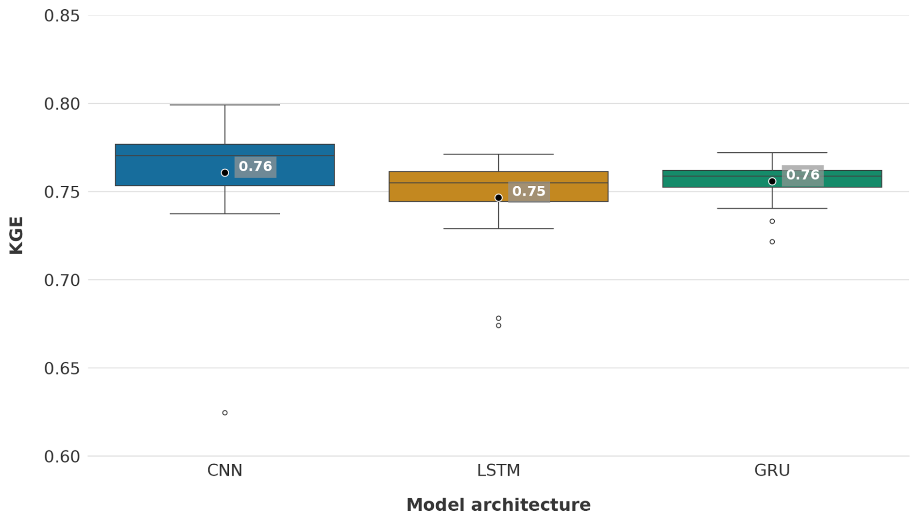
Figure 6 Distribution of KGE values for CNN, LSTM and GRU models across 20 independent runs with different random seeds using a batch size of 256 and incorporating static features. The number represents the average KGE over all 20 runs.

3.2 Runtime

To investigate the computational efficiency associated with the models employed, the runtime of the training process was measured for each model, considering variations in both batch size and the combination of features.

Both the batch size and the integration of additional static features significantly influence the runtime of models across all employed architectures, as evidenced in Fig. 7. The CNN model with a batch size of 2048 and without static features presented the shortest runtime of approximately 2.3 min. Although the CNN model demonstrated rapid convergence towards its optimal minimum error, it simultaneously exhibited the lowest performance as delineated in Fig. 5. This suggests that the conditions were not sufficiently robust to discern the intrinsic patterns.

Using an identical batch size and feature configuration, the GRU model, along with the CNN model configured with a batch size of 256 and no static features, had the second shortest runtimes of approximately 4.2 min.

The introduction of static features resulted in a notable increase in the runtime for all models, barring the GRU model with a batch size of 256, where the inclusion of static features marginally reduced the runtime, rendering it the fastest among all models that utilised static features. The runtime augmentation was especially pronounced in the CNN model with a batch size of 2048, showing a more than 12-fold increase, thereby marking it as the most time-consuming model across all evaluated scenarios. LSTM models also exhibited a substantial increase in runtime across both batch sizes upon the incorporation of static features.

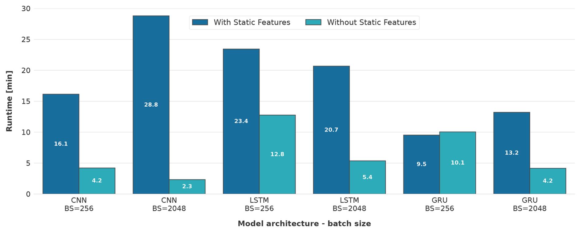
Figure 7 Comparison of model runtime across three different architectures (CNN, LSTM and GRU) with varying batch sizes (256 and 2048) and the presence or absence of static features.

Within identical model architectures, it is observed that larger batch sizes contribute to faster runtimes in the absence of static features. Conversely, when static features are employed, models tend to exhibit faster runtimes with smaller batch sizes, with the exception of the LSTM models. For these models, an escalation in batch size consistently results in accelerated runtimes, irrespective of the feature configuration.

The different behaviour of additional features towards training runtime while using different batch sizes is unexpected and cannot be explained solely by considering the batch size and feature scenarios. As reported by Radiuk (2017), larger batch sizes correlate with increased runtimes, which is attributable to the higher computational utilisation required to process an increased quantity of training samples for the purpose of updating model weights. Nonetheless, this assertion assumes that the models under comparison diverge only in terms of batch and feature size. This presumption does not apply to the present study, where each model is also characterised by a unique optimised combination of hyperparameters (Table 3). A possible explanation might be that all models exhibiting a more protracted runtime require additional epochs to converge. This phenomenon could be facilitated by the early-stopping mechanism deployed in model training, which permits the termination of the training process when the optimised metric ceases to demonstrate improvement.

Altogether, when static features are incorporated, the GRU model utilising a batch size of 256 demonstrates the fastest runtime (9.5 min). In contrast, the CNN model, configured identically with respect to batch size and employed features, exhibited a runtime of 16.1 min, consequently rendering the runtime of the GRU model 41 % faster. In the final analysis, it becomes evident that the GRU model exhibits superior runtime performance compared to both the CNN and LSTM models, specifically when employing a batch size of 256 and utilising static features. In the context of RNN models, with a focus on runtime, GRU models were found to be superior in terms of efficiency compared to LSTM models. This stands in alignment with the findings of Yang et al. (2020), who reported that GRU was 29 % faster than LSTM when processing the identical dataset. However, as stated before, the examined models in this study not only exhibit disparities in terms of batch size but also encompass other architectural parameters such as the number of utilised epochs, hidden units and the window size (Table 6). These differences may result in altered computational efforts.

Apart from the different model architectures, the specific configuration of hyperparameters in each model yields varying computational effort. For example, an increase in window size results in a more extended sequence to process, thereby necessitating additional computational effort. In the context of the CNN models, the computational effort is contingent on the window size, feature maps, kernel size and quantity of input features. Models incorporating static features (+SF) possess 14 input features, whereas those without static features (−SF) contain only 3 dynamic features. In contrast, the computational effort of the LSTM and GRU models is determined by the units within the corresponding cell, the input feature size and the window size.

The observed increase in computational time for the GRU model, when running with a batch size of 256 and no static features, is mainly due to a significantly larger window size, which increased from 87 to 298. This expansion, in the absence of static features, requires a more extensive computational effort. In contrast, for CNN models employing a batch size of 2048, the pronounced augmentation in execution time is primarily induced by an increase in the quantity of feature maps, presenting a 2.3-fold increase. Generally, the marked prolongation in computational duration for CNN models incorporating static features, as opposed to those excluding them, can be elucidated by the incorporation of a considerably higher number of feature maps in the former. This enlargement is a direct consequence of the increased data volume processed by the models when supplemented with static features. Notably, CNN models utilising a batch size of 2048 manifest a reduction in window size, implying that the model may encounter challenges in generalising from extended input sequences due to potentially excessive variability among the samples within a batch.

For the LSTM models with a batch size of 2048, an 83 % increase in the number of hidden units when static features are introduced is the primary factor contributing to the substantial increase in runtime for this configuration. Notably, the GRU model with a batch size of 256 and static features, which exhibits the smallest window size of 87 among all recurrent models, achieves the fastest runtime for models incorporating static features, a result directly attributable to its reduced window size, while still maintaining commendable predictive performance.

Table 6 Selection of utilised hyperparameters for the employed CNN, LSTM and GRU models: a comparative examination of different feature scenarios, including scenarios with static features (+SF) and without static features (−SF), across two distinct batch sizes (256 and 2048).

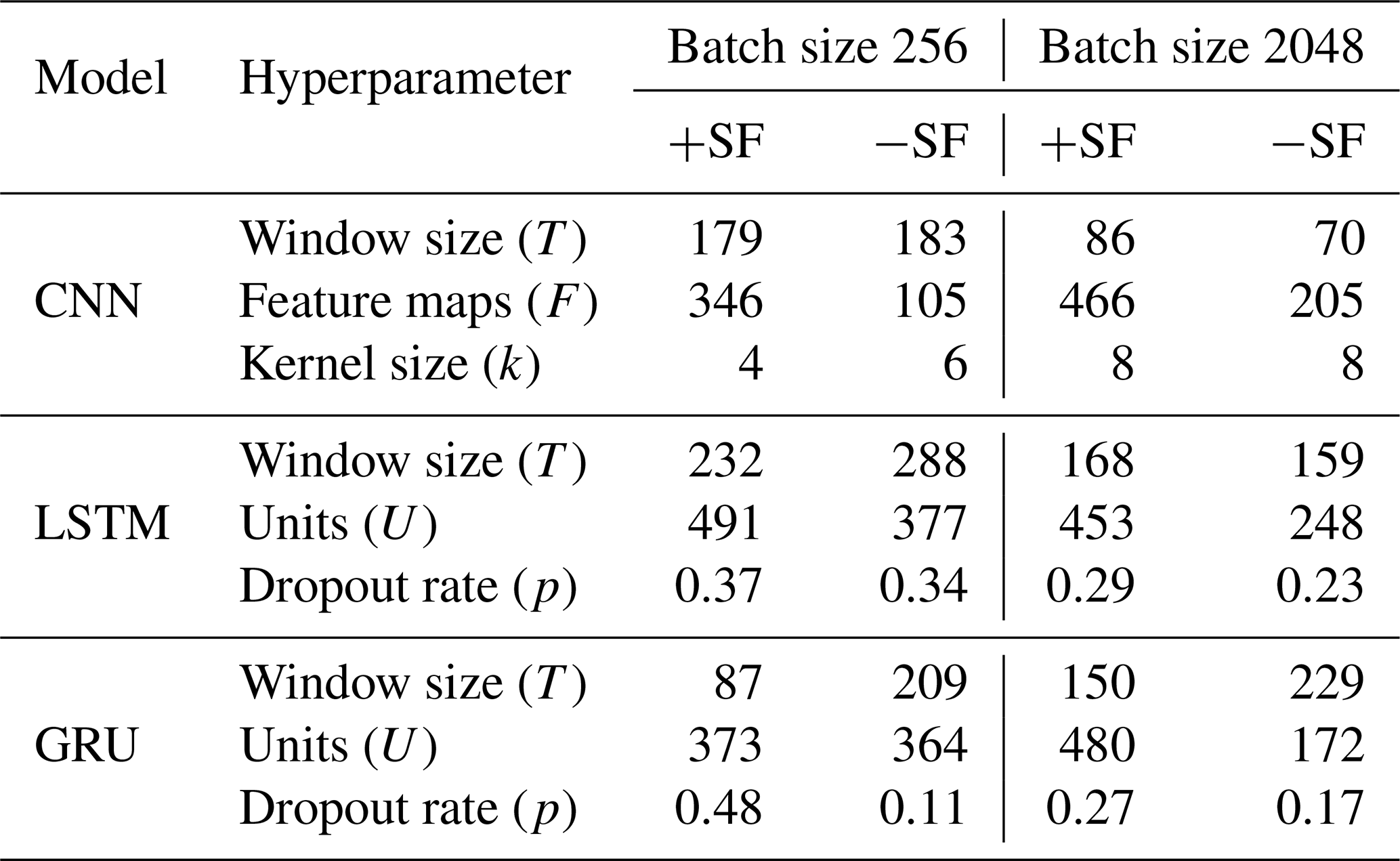
The architectural differences between CNN models and recurrent models (LSTM and GRU) render direct comparisons of their hyperparameter configurations impracticable, with the exception of window size. As indicated in Table 6, the window sizes of CNN models are smaller than those observed in recurrent models, except for the GRU model employing a batch size of 256 and incorporating static features.

Moreover, an assessment of the best-performing models within each architecture (all configured with a batch size of 256 and incorporating static features) reveals that the aforementioned GRU model possesses the smallest window size (87), followed by the CNN (179) and the LSTM (232) models. The increased length of input sequences implies greater computational demands, which partly accounts for the elevated runtime observed in the specified CNN model despite its inherent capacity for parallel processing. As outlined in Sect. 2.5, this attribute is typical of CNN models, whereas the sequential-processing nature of LSTM and GRU models limits such parallelisation.

In conclusion, the comparative analysis suggests that the GRU model, particularly when utilising a batch size of 256 and incorporating static features, emerges as the optimal choice for hydrological applications prioritising computational efficiency alongside predictive performance. Furthermore, the differential impact of batch sizes and feature configurations on the runtime across CNN, GRU and LSTM models underscores the critical role of tailored hyperparameter optimisation in achieving computational efficiency without compromising model performance.

Given the observed favourable outcomes when employing a batch size of 256 with static features, subsequent analyses will focus exclusively on models adhering to this configuration.

Assessment of flow segment performance

To reinforce the analysis of performance, the recorded discharge data from all evaluated catchments, corresponding to the highest-performing model within each architectural category, were divided into quartiles. First, the discharge data for each catchment were sorted in ascending order. Then, the sorted data were divided into four quartiles, with each quartile representing a 25 % portion of the data range for each catchment, thereby forming four distinct segments. Subsequently, for each segment, KGE and PBIAS of the predicted discharge were calculated in relation to the observed values, as illustrated in Fig. 8.

Across all models, a noticeable increase in KGE is observed from the lowest to the highest flow segments, with the exception of Q2, which represents lower flow levels and records the lowest KGE values. Remarkably, only within the highest flows is a positive KGE observed. This implies that the models predominantly discern peak flow events as critical data for learning, treating low flows as less significant or noise, which the models aim to diminish.

This phenomenon may be attributed to a bias in the KGE towards elevated flows, thereby inadequately penalising inaccuracies in lower flow predictions. Specifically, KGE includes three parts, namely the Pearson correlation coefficient r, variability α and bias β (Eq. 1). Because peak flows typically exhibit larger numerical values than lower flows, they might dominate the overall variance; slight improvements in capturing these high-flow events can thus yield relatively large gains in all three components, thereby improving the overall KGE score.

Consequently, forthcoming research should explore evaluation metrics that facilitate a more holistic optimisation approach. Regarding the highest flows, the KGE metrics exhibit close resemblance across models, with the CNN model leading slightly with a KGE of 0.69. Conversely, the LSTM model demonstrates superior efficacy in modelling Q1 and Q2 flow segments.

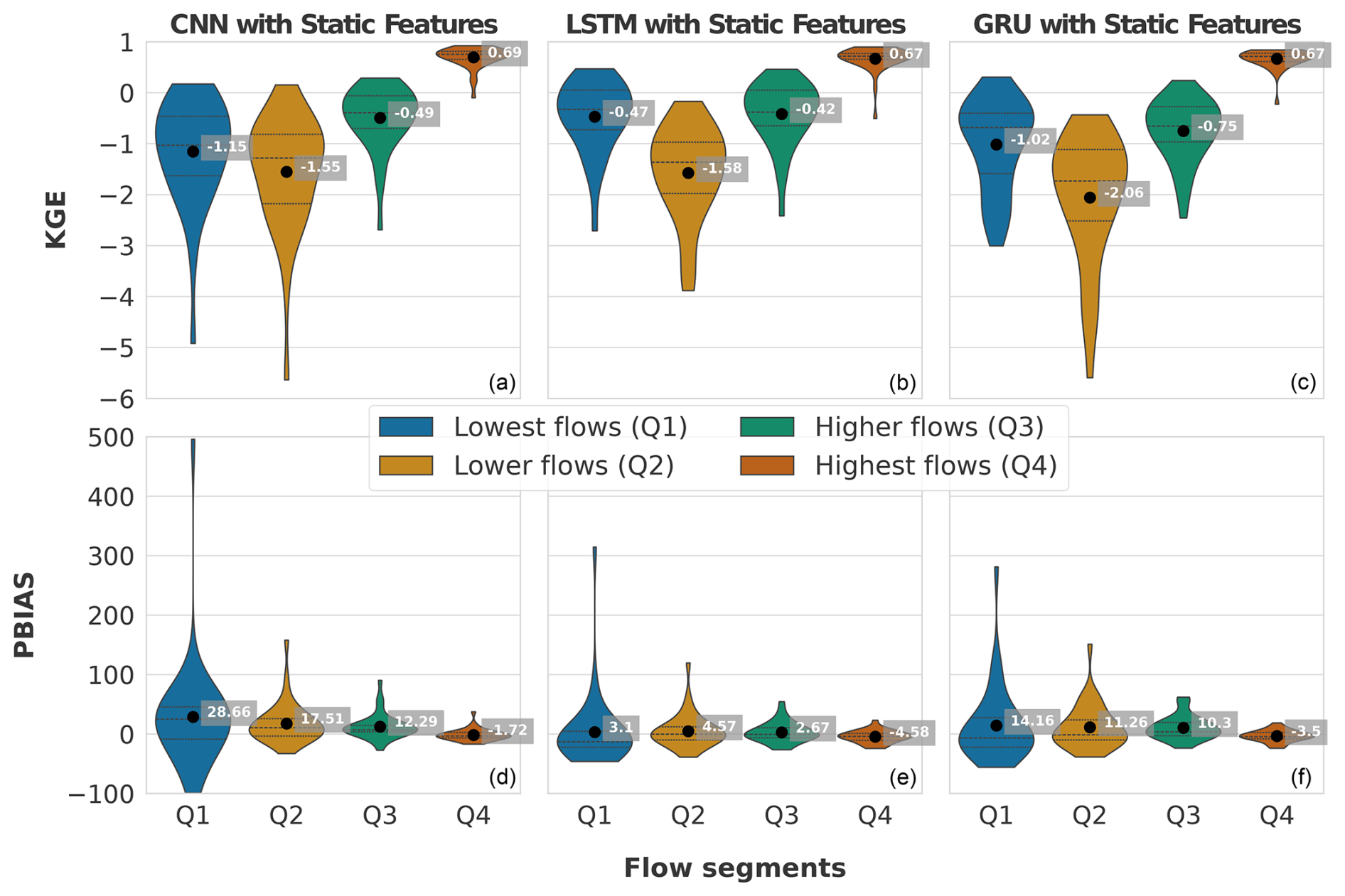
Figure 8 Comparative performance of CNN, LSTM and GRU models incorporating static features across different flow segments. The top row (a–c) displays the Kling–Gupta efficiency (KGE), and the bottom row (d–f) shows the percent bias (PBIAS) for the lowest flows (Q1), lower flows (Q2), higher flows (Q3) and highest flows (Q4). Each violin plot represents the distribution of model performance metrics for all evaluated catchments within each flow segment. The black dots indicate the mean values for each segment.

Addressing the PBIAS, the pattern of enhanced model performance with increasing flow magnitudes, as noted with KGE metrics, persists. This is evidenced by the narrowing spread of the violin plots. Intriguingly, except for the Q4 segment, the PBIAS remains positive across all models for each flow segment, indicating a general overestimation of the lowest to higher flows and a mild underestimation of peak flows. This phenomenon may be attributed to the limitation described in Sect. 2.5.1, whereby the integration of a sigmoid activation function with a min–max scaler inherently limits the highest possible prediction value to the maximum observed during the training phase.

Notably, the predictions by the CNN model for the lowest flow exhibit the most pronounced bias, particularly on the positive spectrum, pointing to a lack of adequate generalisation capabilities.

A further decomposition of the KGE is illustrated in Fig. 9, where each of the three components of the KGE (Pearson correlation coefficient (r), variability (α) and bias (β)) are presented separately. These components offer insights into distinct aspects of the model's performance. The Pearson correlation coefficient (r) measures the strength and direction of the linear relationship between the observed and simulated data. A value of 1 indicates perfect positive correlation, −1 indicates perfect negative correlation, and 0 indicates no correlation. The variability (α) measures the ability of the model to capture the observed variability. A value of 1 indicates that the model's variability matches the observed variability. Values greater than 1 indicate that the model has higher variability, while values less than 1 indicate lower variability. The bias term (β) indicates the systematic overestimation or underestimation by the model. A bias value of 1 means there is no bias, values greater than 1 indicate overestimation, and values less than 1 indicate underestimation.

Figure 9 reveals that r is more consistent across Q1 to Q4 for the LSTM model, unlike the CNN and GRU models, which display a wider range for r below 0.25. This indicates that the LSTM model is better at matching the timing of prediction for low flows. A similar trend is observed for α, where the LSTM and GRU models exhibit higher variability, particularly for the lowest flows (Q1). However, the GRU model shows difficulties in capturing variability for lower and higher flows (Q2 and Q3), with values of 3.96 and 2.63, respectively, compared to the LSTM and CNN models.

The bias term (β) shows that the CNN model achieves the best score for the highest flows (Q4). Nevertheless, it also exhibits the largest bias for the lowest flows (Q1) among all models. Conversely, the LSTM model demonstrates superior performance for Q1 through Q3.

Overall, this analysis suggests that the LSTM model exhibits favourable results across all KGE components. Appendix A presents the three best-performing and three worst-performing hydrographs of each model. Within the poorly performing hydrographs, it becomes evident that, while the timing of the flow events is mostly accurate, the magnitude is poorly captured, and the base flow is often underestimated. This suggests that these catchments might exhibit different hydrological behaviours compared to the better-predicted catchments, indicating the need for more diverse catchments in the training dataset. Furthermore, Appendix A4 presents a comparison of the simulated hydrographs for the same basin. Consistent performance trends are observed across all models, with either poor or high performance in the same basin. However, one plot exhibits mixed performance, where both LSTM and GRU models perform well, while the CNN model shows poor performance. Notably, this is the only validated catchment where such a strong discrepancy is observed.

In summary, the evaluation of flow segment performance has provided valuable insights into the performance distribution. While the CNN model showed superior average performance, as demonstrated within the preceding sections, the LSTM model exhibited a higher degree of consistent performance across all flow segments. Additionally, the recurrent models displayed enhanced generalisation capabilities for the lowest flow rates in each catchment.

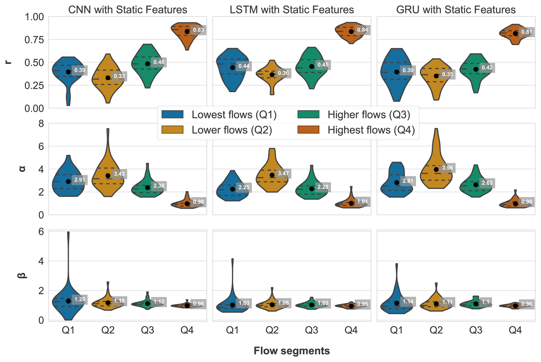
Figure 9 Components of the Kling–Gupta efficiency (KGE) for the employed CNN, LSTM and GRU models with a batch size of 256 and incorporating static features, evaluated across four flow segments: lowest flows (Q1), lower flows (Q2), higher flows (Q3) and highest flows (Q4). From top to bottom, the rows represent the Pearson correlation coefficient (r), the variability ratio (α) and the bias (β). Each violin plot illustrates the distribution of these metrics for all evaluated catchments within each flow segment, with black dots indicating the mean values for each segment. The ideal value for all three metrics is 1, indicating perfect performance.

3.3 Model sensitivity

To elucidate the effect of the input features on discharge prediction, a sensitivity analysis was conducted. For that, each daily input feature was uniformly increased by 10 %, and, subsequently, the prediction was executed again with the modified inputs. The newly predicted discharge values were then systematically averaged over both time and all catchments, resulting in one metric. Variations in the mean discharge resulting from these adjustments yield insights into the comparative significance of each evaluated feature within the model. This analysis focuses solely on dynamic features due to the limited number of catchments (35). With only 35 samples for static features, the models lack sufficient variability in the input to reliably interpret these features.

The results of this analysis are shown in Fig. 10, representing the mean percentage change in discharge, calculated by averaging over all daily predictions and across all 35 catchments.

For the CNN model, the meteorological feature precipitation exhibited the most positive impacts on the model, with changes of 11.1 % (Fig. 10a). This underscores its pivotal role in influencing the output of the CNN model. Increasing the daily feature soil temperature led to a decline in discharge of −2 %, likely related to increasing atmospheric water losses with rising temperature through increasing actual soil evaporation and plant transpiration. The daily forcing evapotranspiration showed a small positive impact of 0.4 %. The observation that daily evapotranspiration increases with discharge is seemingly counterintuitive. However, daily evapotranspiration derived from Jehn et al. (2021) represents actual evapotranspiration, which can increase with wetter conditions and therefore also correlate positively with discharge.

Although this may offer a plausible explanation for the observed anomalous behaviour, it is unlikely within the context of this study. Given that all models share the same input features, both the LSTM and GRU models should exhibit similar behaviour, which is not observed (see Fig. 10).

Analogously to the findings from the CNN model analysis, the LSTM model further corroborated the fact that precipitation exerts the most substantial positive impacts on discharge, registering enhancements of 15 % (Fig. 10b). Conversely, daily sum evapotranspiration negatively impacted discharge, resulting in decreases of −2.2 %. In comparison to the CNN model, the LSTM model displays a substantially higher sensitivity to precipitation, implying that this feature serves as the principal driving force for this model. The daily feature soil temperature revealed a decrease of −3.3 %.

The sensitivity analysis of the GRU model parallels the findings of the LSTM model. Precipitation exerts strong positive effects on discharge, with increases of 13.3 % (Fig. 10c). Evapotranspiration demonstrated a negative impact on discharge by −3.1 %. This makes the GRU model the most sensitive to this feature. The soil temperature exhibited a uniform reduction in discharge of −3.3 %.

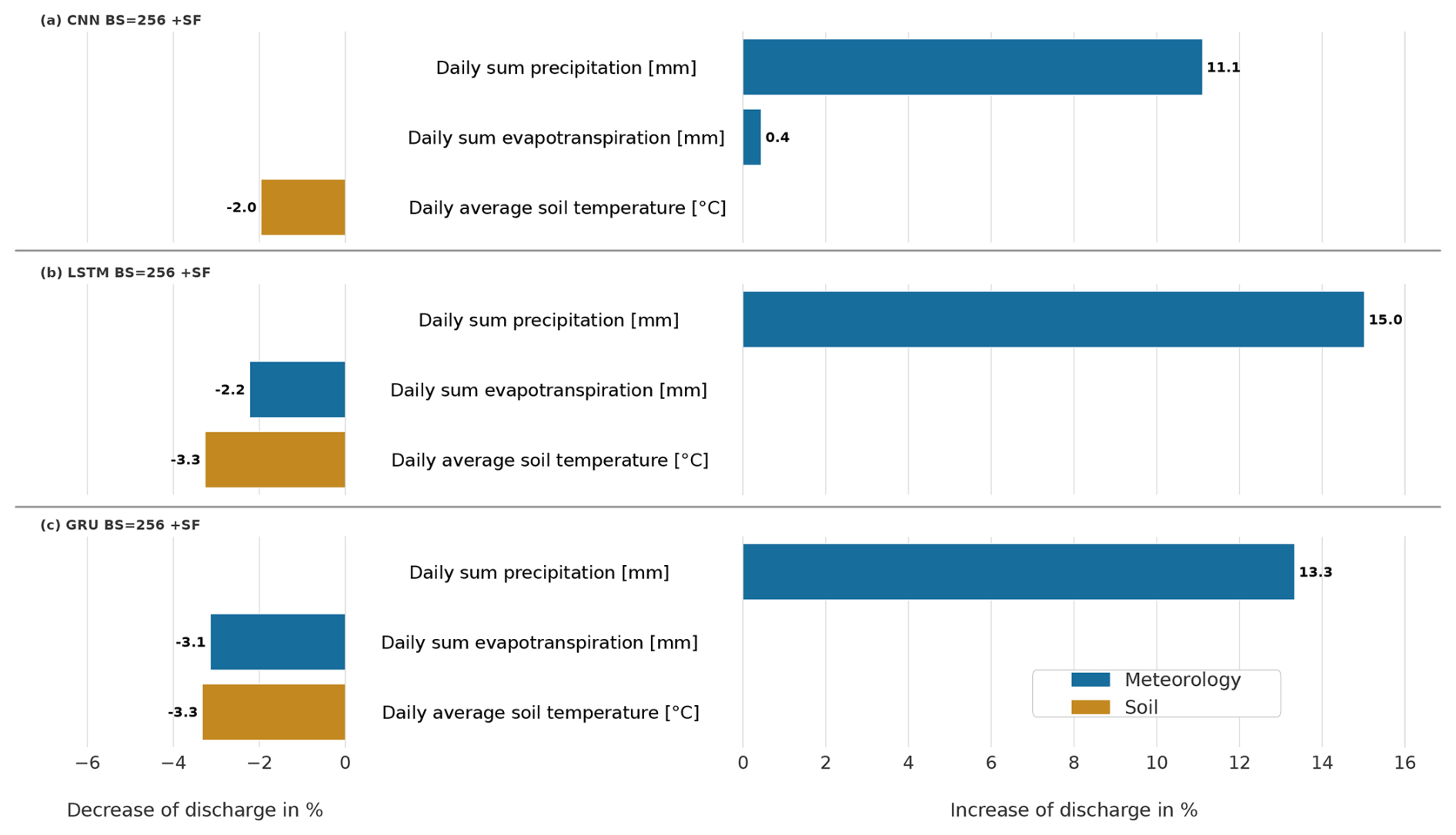
Figure 10 Sensitivity analysis of the CNN (a), LSTM (b) and GRU (c) models with static features and a batch size of 256. All features have been uniformly increased by 10 % to evaluate their impact on discharge prediction.

In summary, the GRU model's sensitivity analysis reveals a high degree of concordance with the LSTM model in terms of feature influences on discharge predictions. All daily input features of these two models exhibited expected behaviours, aligning with established hydrological principles. This indicates a robust understanding of the input features' influences by both models.

The similarity in effects across all input features suggests that GRU models are also adept at accurately discerning hydrological processes despite their simpler architecture compared to LSTM models. The CNN model exhibits counterintuitive results with the daily evapotranspiration feature, indicating potential limitations in handling these inputs, although it is possible that certain static features had a greater influence on this model's performance.

Overall, the sensitivity analysis of the LSTM and GRU models revealed a more realistic representation for evapotranspiration compared to the CNN model. These findings emphasise the importance of considering various input parameters and their interactions in improving discharge prediction models for hydrological applications.

4 Conclusions

This study conducted a comparative evaluation of CNN, LSTM and GRU models for predicting daily discharge in ungauged basins across Hesse, Germany. All three deep-learning architectures exhibited significant predictive capabilities. Specifically, the CNN model yielded marginally higher accuracy (KGE = 0.8) compared to the recurrent models, effectively capturing local short-term rainfall–runoff dynamics. Conversely, the LSTM model (KGE = 0.78) demonstrated superior consistency across the entire flow spectrum, maintaining balanced performance from low to high flows rather than disproportionately excelling at peak events, as observed with CNN models. The GRU model (KGE = 0.77) provided a robust balance between computational efficiency and predictive accuracy. The minor performance gaps observed indicate that no single architecture dominates significantly in terms of predictive skills.

Consistently with the findings of Kratzert et al. (2019a), augmenting models with static catchment attributes improved prediction performance, underscoring the critical importance of integrating catchment-specific information into ungauged basin modelling. Additionally, models trained with smaller batch sizes yielded better KGE scores compared to larger batch sizes, suggesting that optimisation dynamics such as gradient noise and update frequency substantially influenced generalisation performance. These results reinforce existing evidence that modern deep-learning methods achieve robust streamflow predictions even in data-scarce basins (Nabipour et al., 2020; Afzaal et al., 2019).

Evaluation across varying flow conditions further revealed that the model architecture substantially influenced the prediction accuracy of peak and low-flow events. The LSTM demonstrated superior generalisation across lowest-flow conditions, indicating reduced systematic errors during extended dry spells. This generalisation capability can be attributed to the LSTM model's gated recurrent structure, effectively capturing long-term dependencies associated with baseflow and recession periods. Conversely, the CNN model employs fixed-size convolutional filters optimised for identifying short-term flow patterns, particularly sharp increases from precipitation events, but exhibited limited capability in terms of capturing slower hydrological processes such as evapotranspiration-driven drawdown.

Sensitivity analyses confirmed precipitation to be the primary discharge driver across all models. However, CNN models showed reduced sensitivity to daily evapotranspiration signals. This characteristic suggests that the CNN architecture may inadequately represent cumulative drying effects, potentially explaining its comparatively weaker performance during low-flow periods. These architectural distinctions highlight how internal model designs significantly affect learned hydrological behaviours. Recurrent networks inherently integrate temporal information, aiding the modelling of sustained processes, whereas convolution-based models may necessitate additional mechanisms or expanded receptive fields to achieve equivalent long-term awareness. Despite these nuances, CNN models still attained the highest aggregate accuracy (KGE), suggesting that accurate peak-flow predictions compensated for deficits in low-flow estimations. Consequently, alternative metrics focused specifically on low-flow performance might rank the LSTM ahead of the CNN.

Regarding computational efficiency, clear distinctions emerged. The GRU model trained significantly faster (over 40 % runtime reduction compared to the CNN model and nearly 60 % faster runtime than the LSTM model), attributable to its streamlined gating mechanism, with fewer parameters and simpler operations (Chung et al., 2014). CNN models, despite being marginally slower than GRU models, benefited from parallelisable convolutional operations and exhibited competitive runtimes coupled with the highest accuracy. In contrast, LSTM models' sequential processing and complex gating incurred greater computational demands (Goodfellow et al., 2016). Additionally, Ebtehaj and Bonakdari (2024) reported an equivalent performance of LSTM and CNN models for high-precipitation events yet observed that CNN models outperformed LSTM models for significant precipitation events at short lead times, thereby reinforcing our results.

Furthermore, our findings align with recent literature on data-driven streamflow forecasting. Oliveira et al. (2023) similarly reported superior CNN model performance relative to LSTM and multilayer perceptron models within calibrated basins. However, that result, obtained from a calibrated basin, did not guarantee broader generalisability. Our multi-basin study confirms CNN model efficacy even in ungauged basins, alongside consistently strong performances by LSTM and GRU models. The minor accuracy differences align with Farfán-Durán and Cea (2024), emphasising context-dependent model performance. For example, the GRU model excelled at very short lead times in one basin (Spain), whereas, in another basin, CNN, LSTM and GRU models performed comparably. Additionally, the computational efficiency advantages observed for GRU and CNN models corroborate prior studies, highlighting parallelism and simplified gating mechanisms as significant computational benefits. Nonetheless, GRU models' simplified gating may reduce performance relative to LSTM models as Wegayehu and Muluneh (2023) demonstrated that LSTM models generally outperform GRU models regardless of input data.

Certain design choices and limitations must be acknowledged. Both recurrent models (LSTM and GRU) constrained outputs to non-negative discharges within the training-data range using sigmoid activation and min–max normalisation. This constraint ensures physically plausible predictions but restricts extrapolation beyond maximum observed flows. This saturation effect may attenuate extreme flood peaks, limiting the model's extrapolation capacity. For practical applications requiring accurate flood forecasting (primarily focusing on high discharge), alternative activation functions such as LeakyReLU, which allow unbounded outputs, may offer greater flexibility and should be considered in future model designs.

Furthermore, our analysis was confined to Hesse, Germany, potentially limiting generalisability to different hydro-climatic contexts such as arid or monsoon climates. Hybrid or ensemble models combining CNN and LSTM layers were outside the scope of this comparison.

Future research should explore loss functions better aligned with hydrological objectives and sequence length handling through longer sliding windows or emerging self-attention transformers (Lim et al., 2021). Investigating architectures that seamlessly fuse static and dynamic inputs via attention mechanisms or dedicated subnetworks could improve the use of catchment attributes and remote sensing data, thereby enhancing generalisation (Lim et al., 2021).

These insights serve as guidance for researchers utilising neural networks in hydrology and contribute to a comprehensive framework for evaluating algorithms. By systematically comparing CNN, LSTM and GRU models in multiple ungauged basins, this work bridges a critical gap in hydrological modelling literature and paves the way for more informed and effective application of artificial intelligence in hydrology. In summary, successful prediction in ungauged basins accentuates the potential of neural networks in advancing streamflow forecasting.

Appendix A

A1 Hydrographs of the CNN model with static features and batch size of 256

A1.1 Highest performance

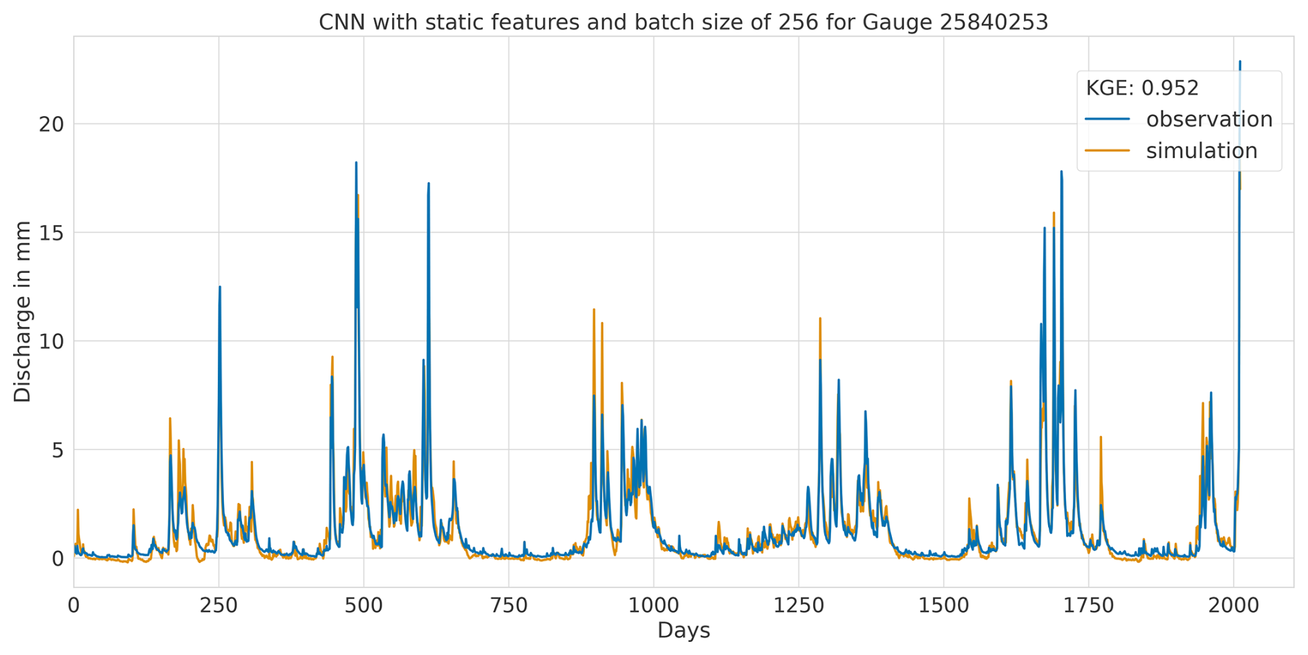
Figure A1 Hydrograph at gauge no. 25840253 illustrating high performance of the CNN model, with observed discharge (blue) and predicted discharge (orange), evaluated using the Kling–Gupta efficiency (KGE).

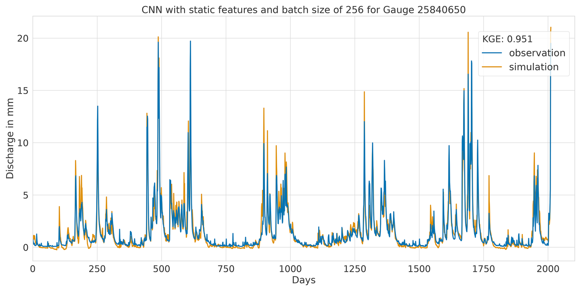
Figure A2 Hydrograph at gauge no. 25840650 illustrating high performance of the CNN model, with observed discharge (blue) and predicted discharge (orange), evaluated using the Kling–Gupta efficiency (KGE).

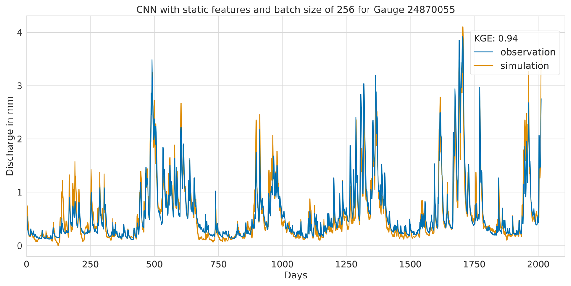
Figure A3 Hydrograph at gauge no. 24870055 illustrating high performance of the CNN model, with observed discharge (blue) and predicted discharge (orange), evaluated using the Kling–Gupta efficiency (KGE).

A1.2 Lowest performance

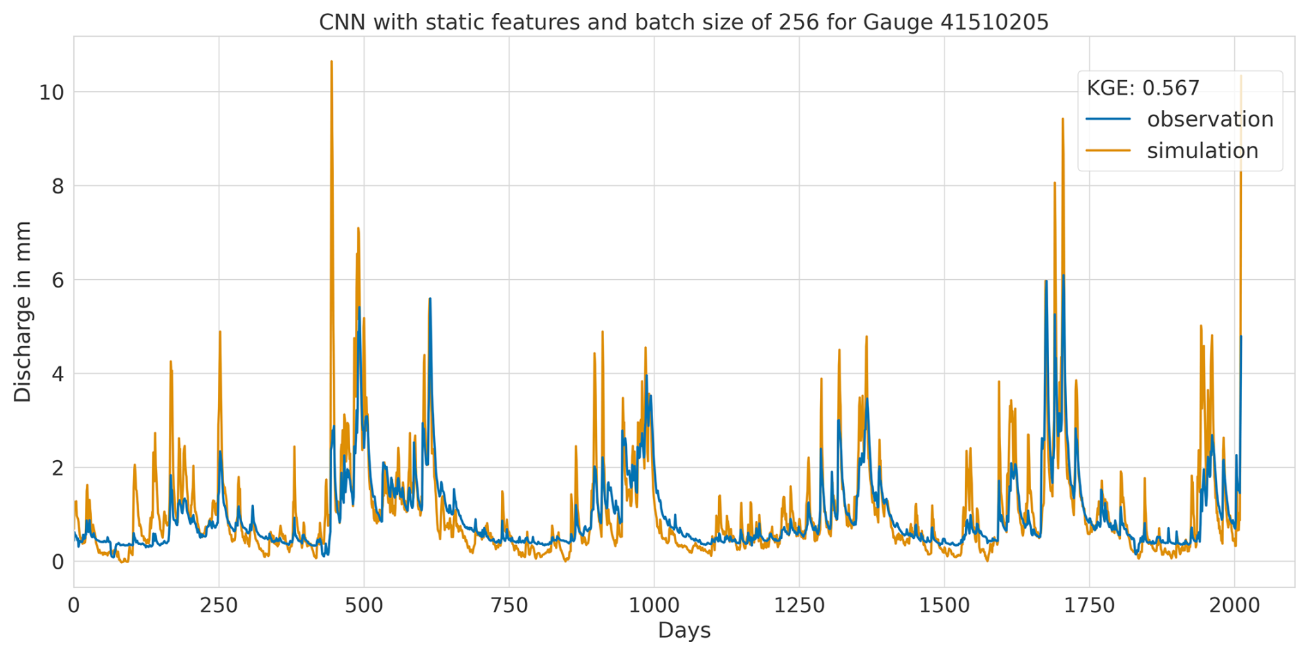
Figure A4 Hydrograph at gauge no. 41510205 illustrating low performance of the CNN model, with observed discharge (blue) and predicted discharge (orange), evaluated using the Kling–Gupta efficiency (KGE).

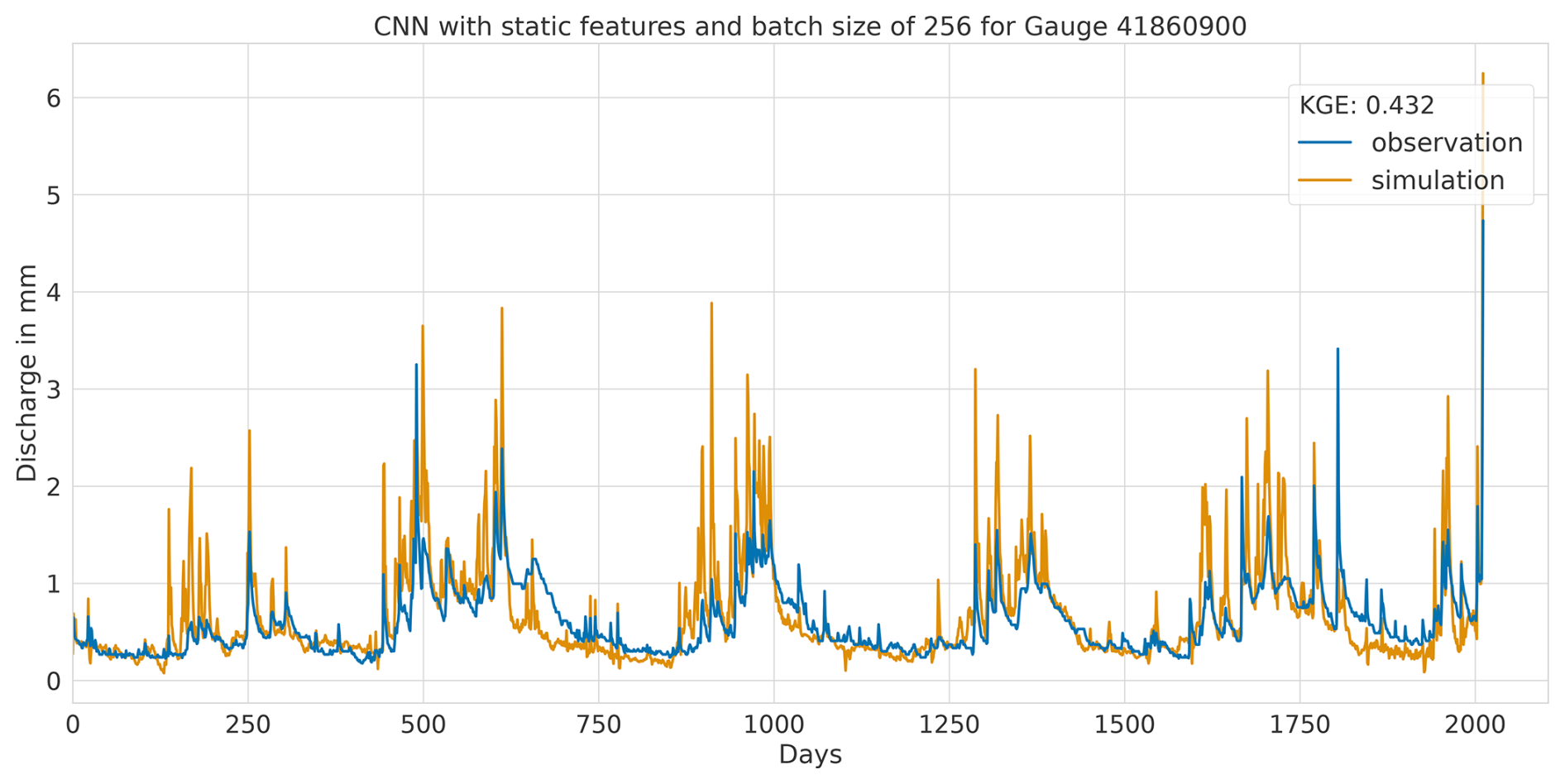
Figure A5 Hydrograph at gauge no. 41860900 illustrating low performance of the CNN model, with observed discharge (blue) and predicted discharge (orange), evaluated using the Kling–Gupta efficiency (KGE).

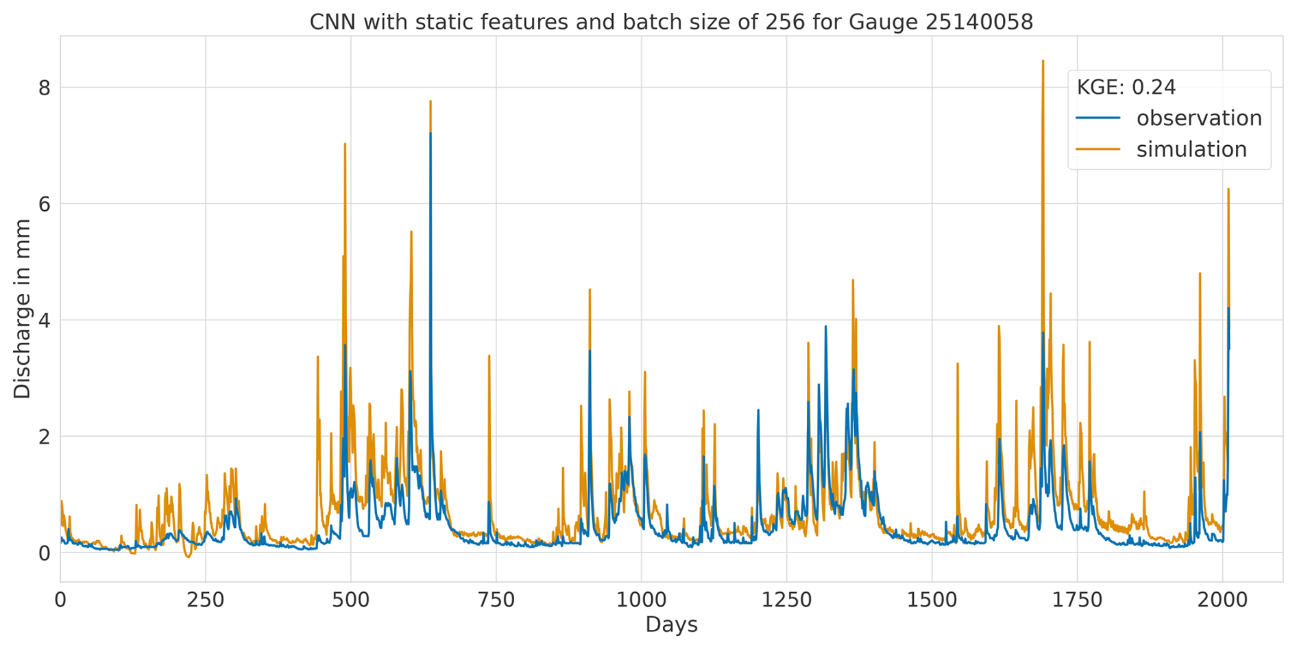
Figure A6 Hydrograph at gauge no. 25140058 illustrating low performance of the CNN model, with observed discharge (blue) and predicted discharge (orange), evaluated using the Kling–Gupta efficiency (KGE).

A2 Hydrographs of the LSTM model with static features and batch size of 256

A2.1 Highest performance

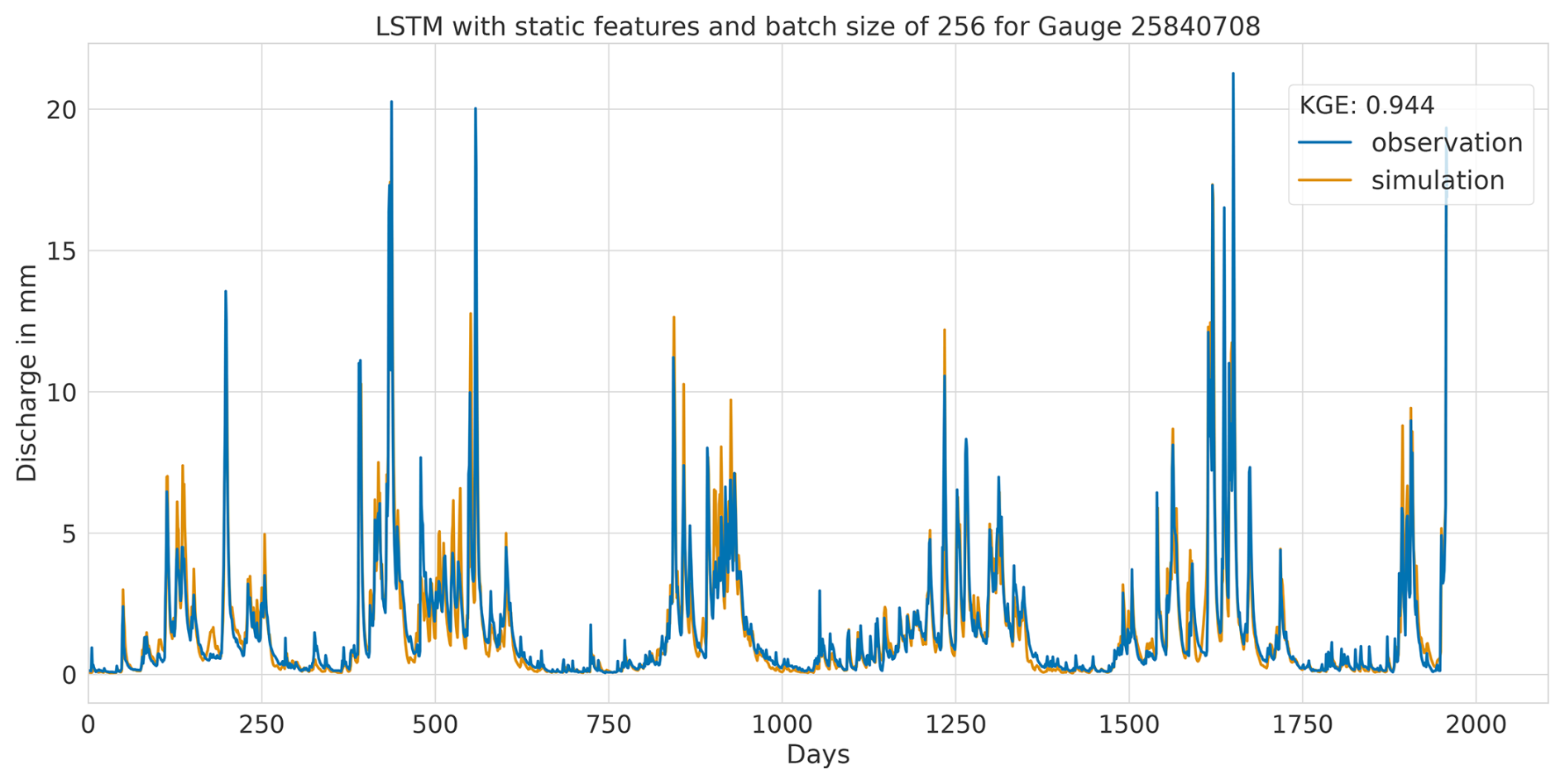
Figure A7 Hydrograph at gauge no. 25840708 illustrating high performance of the LSTM model, with observed discharge (blue) and predicted discharge (orange), evaluated using the Kling–Gupta efficiency (KGE).

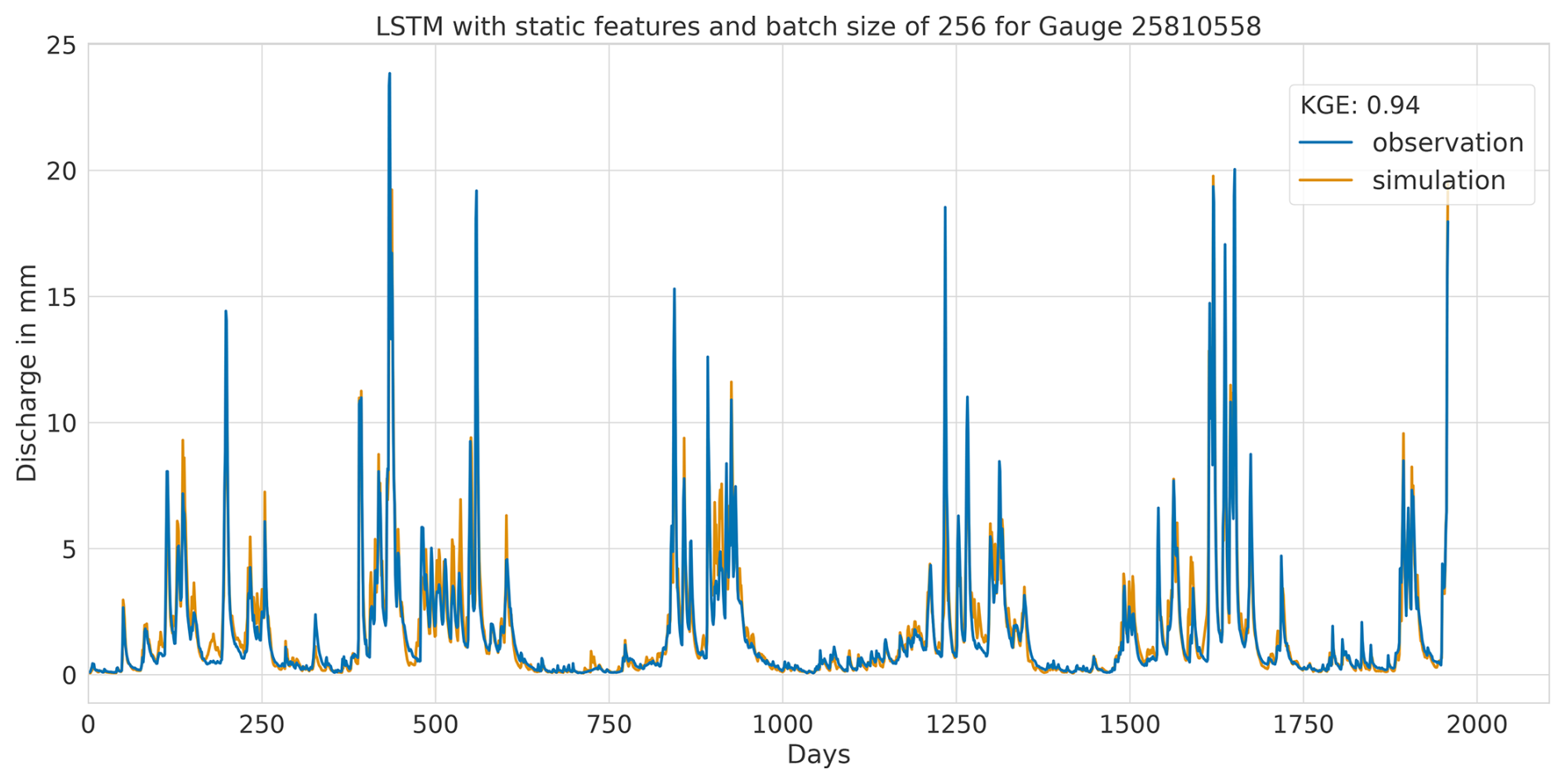
Figure A8 Hydrograph at gauge no. 25810558 illustrating high performance of the LSTM model, with observed discharge (blue) and predicted discharge (orange), evaluated using the Kling–Gupta efficiency (KGE).

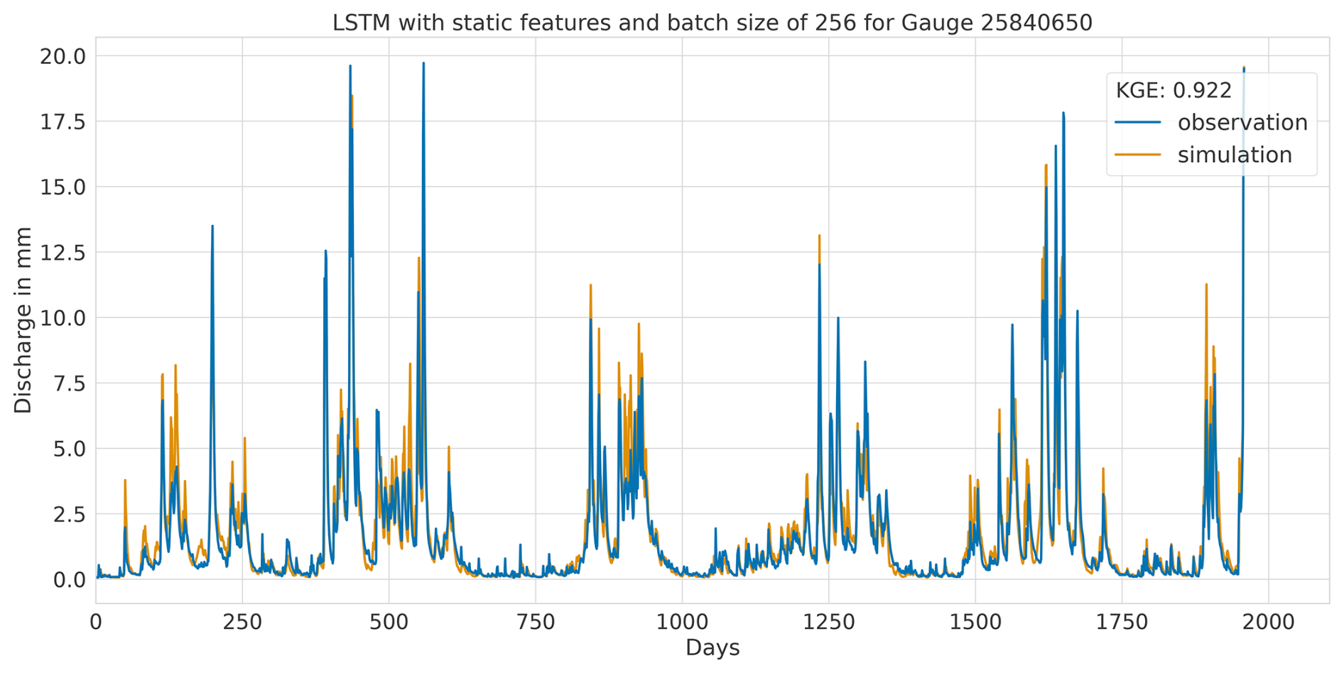
Figure A9 Hydrograph at gauge no. 25840650 illustrating high performance of the LSTM model, with observed discharge (blue) and predicted discharge (orange), evaluated using the Kling–Gupta efficiency (KGE).

A2.2 Lowest performance

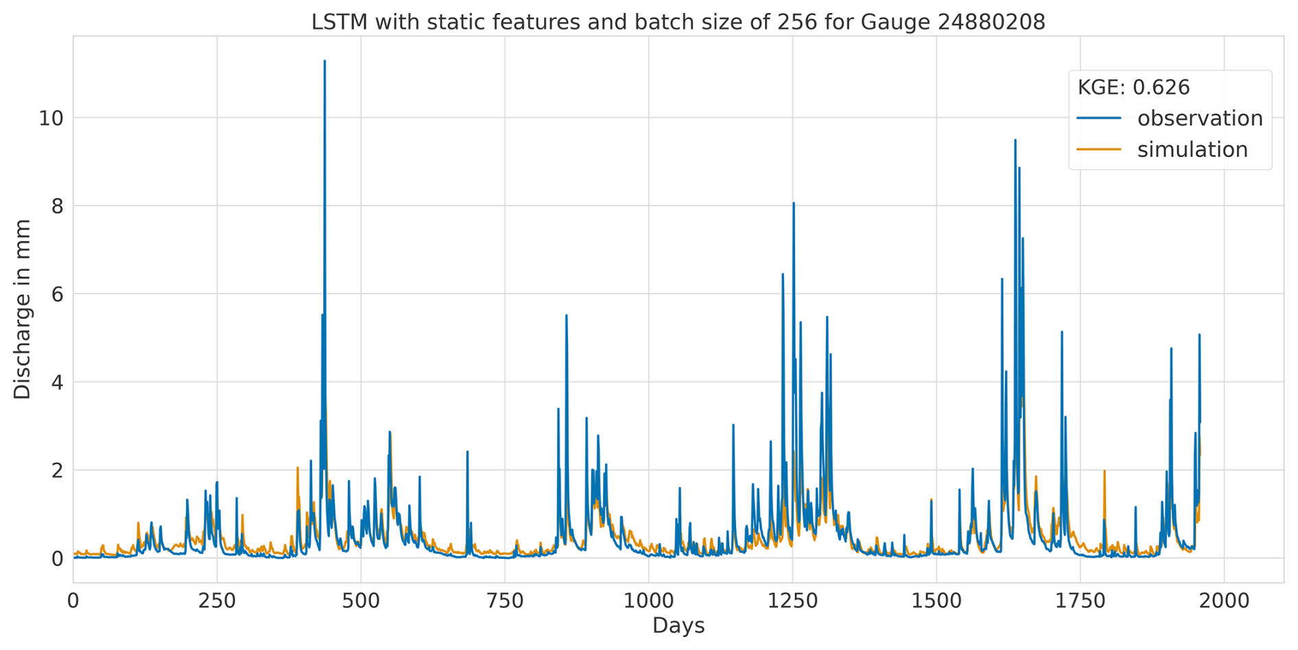
Figure A10 Hydrograph at gauge no. 24880208 illustrating low performance of the LSTM model, with observed discharge (blue) and predicted discharge (orange), evaluated using the Kling–Gupta efficiency (KGE).

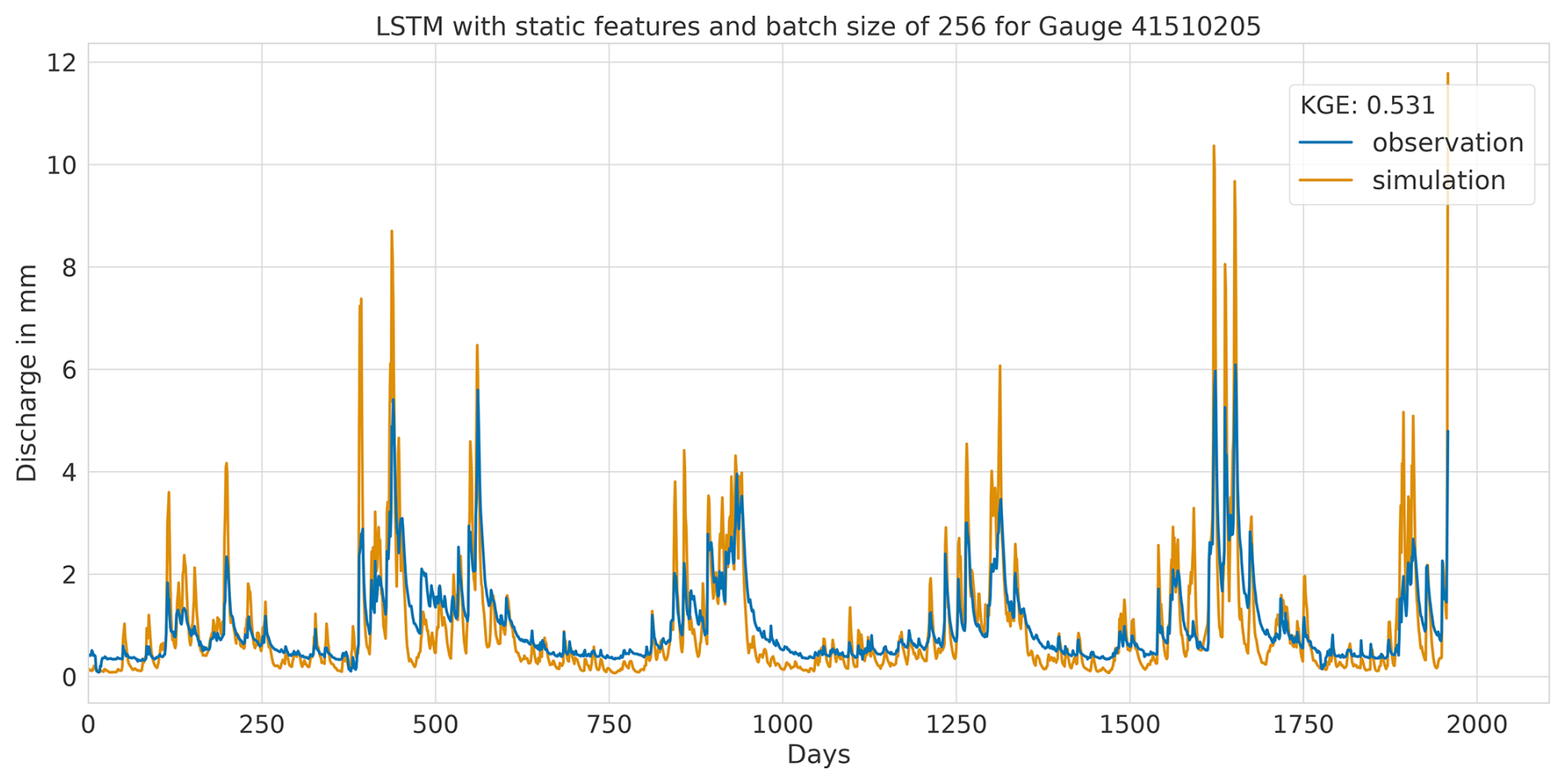
Figure A11 Hydrograph at gauge no. 41510205 illustrating low performance of the LSTM model, with observed discharge (blue) and predicted discharge (orange), evaluated using the Kling–Gupta efficiency (KGE).

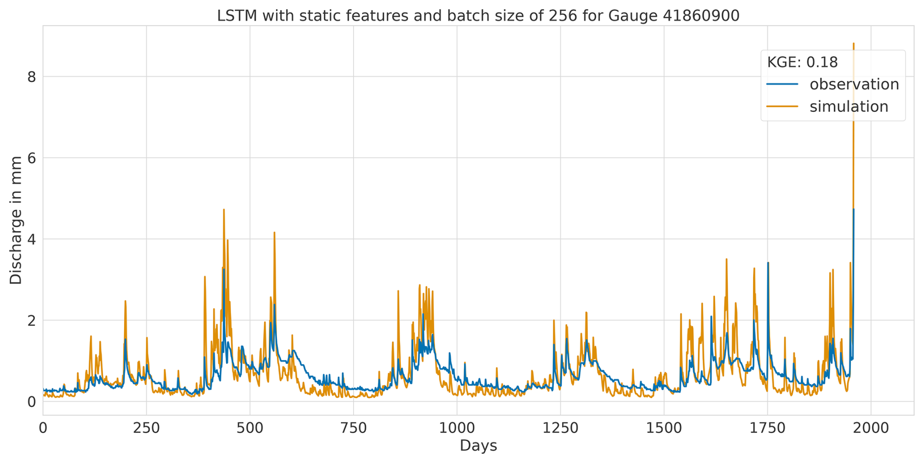
Figure A12 Hydrograph at gauge no. 41860900 illustrating low performance of the LSTM model, with observed discharge (blue) and predicted discharge (orange), evaluated using the Kling–Gupta efficiency (KGE).

A3 Hydrographs of the GRU model with static features and batch size of 256

A3.1 Highest performance

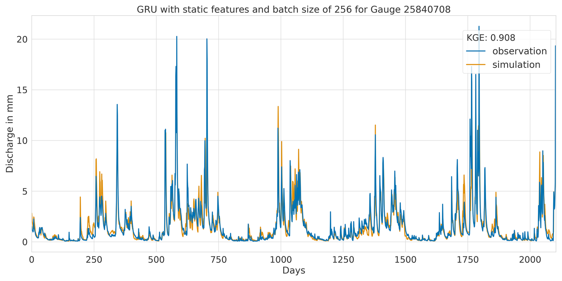
Figure A13 Hydrograph at gauge no. 25840708 illustrating high performance of the GRU model, with observed discharge (blue) and predicted discharge (orange), evaluated using the Kling–Gupta efficiency (KGE).

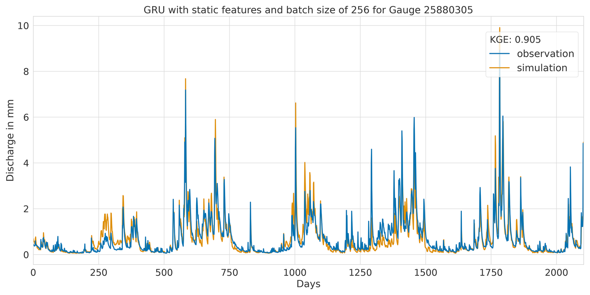
Figure A14 Hydrograph at gauge no. 25880305 illustrating high performance of the GRU model, with observed discharge (blue) and predicted discharge (orange), evaluated using the Kling–Gupta efficiency (KGE).

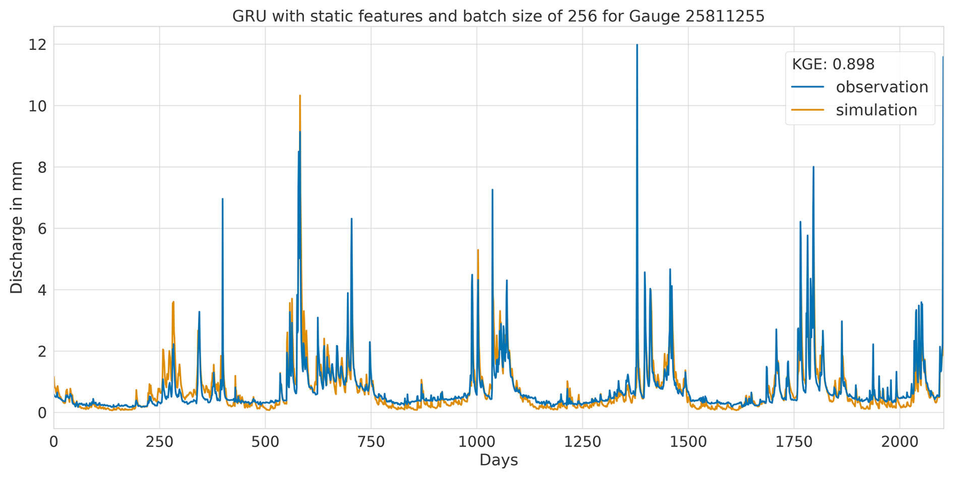
Figure A15 Hydrograph at gauge no. 25811255 illustrating high performance of the GRU model, with observed discharge (blue) and predicted discharge (orange), evaluated using the Kling–Gupta efficiency (KGE).

A3.2 Lowest performance

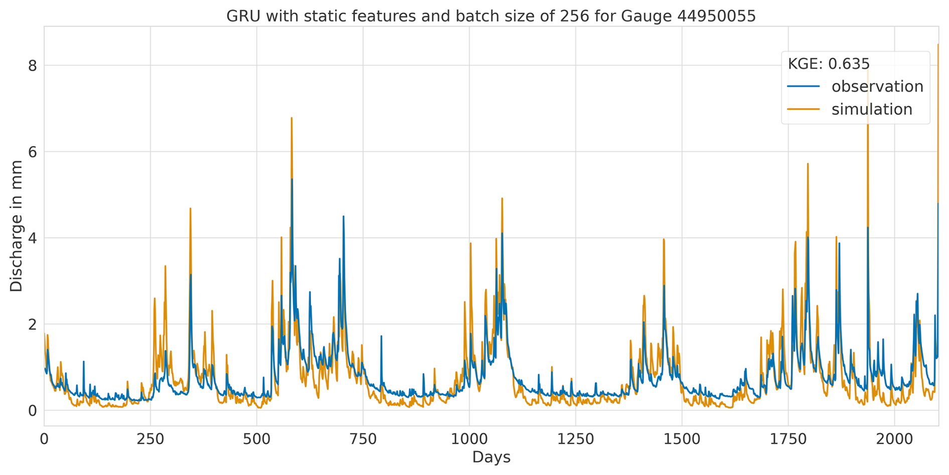
Figure A16 Hydrograph at gauge no. 44950055 illustrating low performance of the GRU model, with observed discharge (blue) and predicted discharge (orange), evaluated using the Kling–Gupta efficiency (KGE).

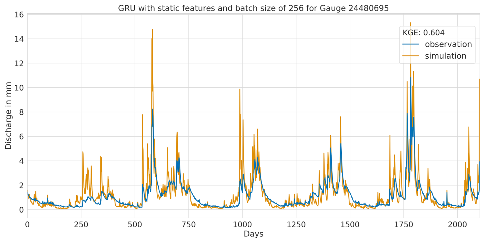
Figure A17 Hydrograph at gauge no. 24480695 illustrating low performance of the GRU model, with observed discharge (blue) and predicted discharge (orange), evaluated using the Kling–Gupta efficiency (KGE).

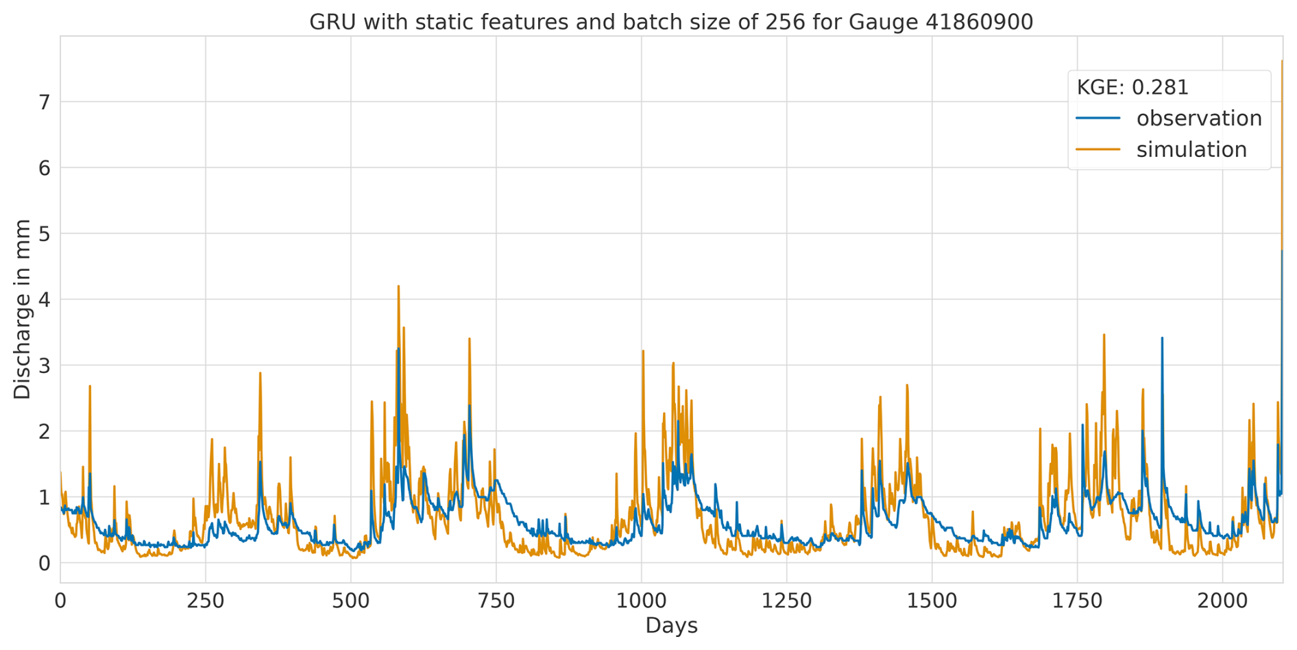
Figure A18 Hydrograph at gauge no. 41860900 illustrating low performance of the GRU model, with observed discharge (blue) and predicted discharge (orange), evaluated using the Kling–Gupta efficiency (KGE).

A4 Hydrograph comparison of the best-performing models with static features and batch size of 256

A4.1 Mixed performance

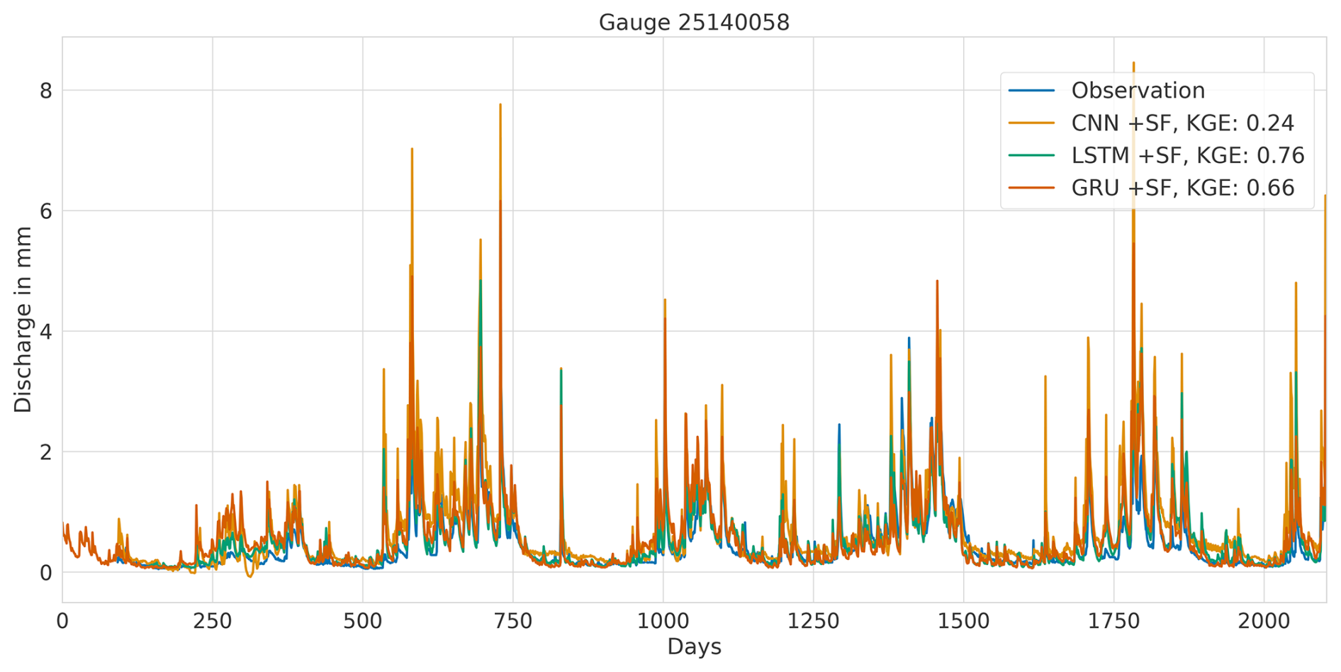
Figure A19 Hydrograph comparison at gauge no. 25140058 for the CNN, LSTM and GRU models, highlighting varying performance across the models. Performance is measured using the Kling–Gupta efficiency (KGE), with “+SF” denoting the inclusion of static features.

A4.2 High performance for all models

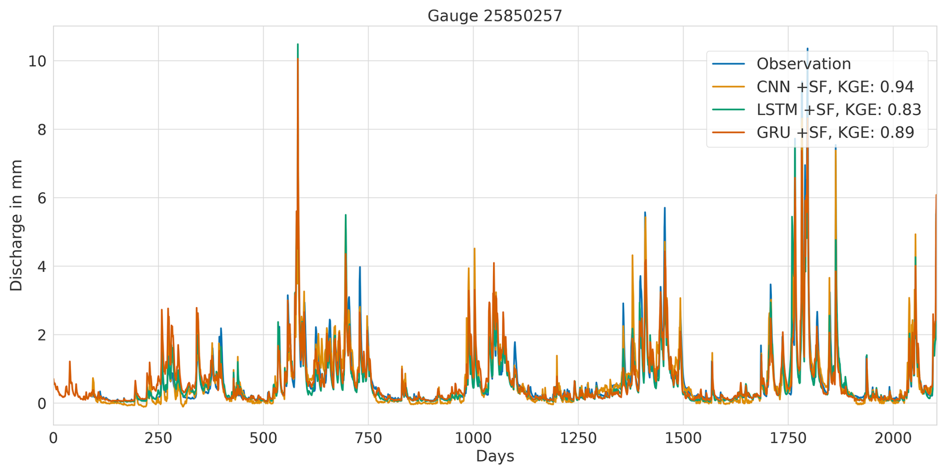
Figure A20 Hydrograph comparison at gauge no. 25850257 for the CNN, LSTM and GRU models, illustrating uniformly high performance across all models. Performance is quantified using the Kling–Gupta efficiency (KGE), with “+SF” indicating the integration of static features.

A4.3 Low performance of all models

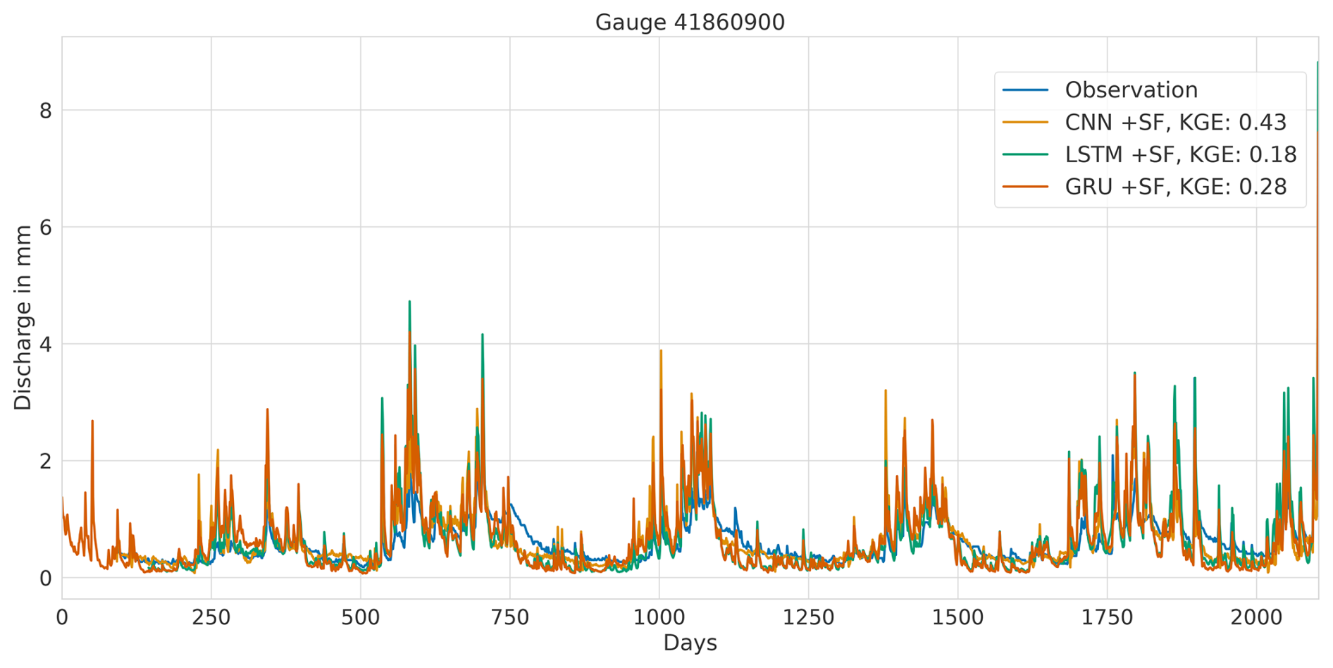
Figure A21 Hydrograph comparison at gauge no. 41860900 for the CNN, LSTM and GRU models, illustrating uniformly low performance across all models. Performance is quantified using the Kling–Gupta efficiency (KGE), with “+SF” indicating the integration of static features.