the Creative Commons Attribution 4.0 License.
the Creative Commons Attribution 4.0 License.
 | 24 Jan 2020
On the configuration and initialization of a large-scale hydrological land surface model to represent permafrost
Mohamed E. Elshamy
Daniel Princz
Gonzalo Sapriza-Azuri
Mohamed S. Abdelhamed
Al Pietroniro
Howard S. Wheater
Saman Razavi
Permafrost is an important feature of cold-region hydrology, particularly in river basins such as the Mackenzie River basin (MRB), and it needs to be properly represented in hydrological and land surface models (H-LSMs) built into existing Earth system models (ESMs), especially under the unprecedented climate warming trends that have been observed. Higher rates of warming have been reported in high latitudes compared to the global average, resulting in permafrost thaw with wide-ranging implications for hydrology and feedbacks to climate. The current generation of H-LSMs is being improved to simulate permafrost dynamics by allowing deep soil profiles and incorporating organic soils explicitly. Deeper soil profiles have larger hydraulic and thermal memories that require more effort to initialize. This study aims to devise a robust, yet computationally efficient, initialization and parameterization approach applicable to regions where data are scarce and simulations typically require large computational resources. The study further demonstrates an upscaling approach to inform large-scale ESM simulations based on the insights gained by modelling at small scales. We used permafrost observations from three sites along the Mackenzie River valley spanning different permafrost classes to test the validity of the approach. Results show generally good performance in reproducing present-climate permafrost properties at the three sites. The results also emphasize the sensitivity of the simulations to the soil layering scheme used, the depth to bedrock, and the organic soil properties.
- Article
(11122 KB) - Full-text XML
-
Supplement
(1140 KB) - BibTeX
- EndNote


Earth system models (ESMs) are widely used to project climate change, and they show a current global warming trend that is expected to continue during the 21st century and beyond (IPCC, 2014). Higher rates of warming have been observed in high latitudes compared to the global average (DeBeer et al., 2016; McBean et al., 2005), resulting in permafrost thaw with implications for soil moisture, hydraulic connectivity, streamflow seasonality, land subsidence, and vegetation (Walvoord and Kurylyk, 2016). Recent analyses provided by Environment and Climate Change Canada (Zhang et al., 2019) have shown that Canada's far north has already seen an increase in temperature of double the global average, with some portion of the Mackenzie River basin (MRB) already heating up by 4 ∘C between 1948 and 2016. Subsequent impacts on water resources in the region, however, are not so clear. Recent analysis of trends in Arctic freshwater inputs (Durocher et al., 2019) highlights that Eurasian rivers show a significant annual discharge increase during the 1975–2015 period, while in North America, only rivers flowing into the Hudson Bay region in Canada show a significant annual discharge change during that same period. Those rivers in Canada flowing directly into the Arctic, of which the Mackenzie River provides the majority of flow, show very little change at the annual scale. However, while the annual scale change may be small, larger changes have been reported at the seasonal scale for northern Canada (St. Jacques and Sauchyn, 2009; Walvoord and Striegl, 2007) and northeastern China (Duan et al., 2017). In the most recent assessment of climate change impacts on Canada, Bonsal et al. (2019) reported that higher winter flows, earlier spring flows, and lower summer flows were observed for some Canadian rivers. However, they also state that “It is uncertain how projected higher temperatures and reductions in snow cover will combine to affect the frequency and magnitude of future snowmelt-related flooding”.
As permafrost underlies about one quarter of the exposed land in the Northern Hemisphere (Zhang et al., 2008), it is imperative to study and accurately model its behaviour under current and future climate conditions. Knowledge of permafrost conditions (temperature, active-layer thickness – ALT, and ground ice conditions) and their spatial and temporal variations is critical for the planning of development in northern Canada (Smith et al., 2007) and other Arctic environments. The hydrological response of cold regions to climate change is highly uncertain, due to a large extent to our limited understanding and representation of how the different hydrologic and thermal processes interact, especially under changing climate conditions. Despite advances in cold-region process understanding and modelling at the local scale (e.g. Pomeroy et al., 2007), their upscaling and systematic evaluation over large domains remain rather elusive. This is largely due to a lack of observational data, the local nature of these phenomena, and the complexity of cold-region systems. Hydrological response and land-surface feedbacks in cold regions are generally complex and depend on a multitude of interrelated factors including changes to precipitation intensity, timing, and phase as well as soil composition and hydraulic and thermal properties.
There have been extensive regional and global modelling efforts focusing on permafrost (refer to Riseborough et al., 2008; Walvoord and Kurylyk, 2016 for a review), using thermal models (e.g. Wright et al., 2003), global hydrological models coupled to energy balance models (e.g. Zhang et al., 2012) and, most notably, land surface models (e.g. Lawrence and Slater, 2005). These studies, however, have typically focused on and modelled only a shallow soil column in the order of a few metres. For example, the Canadian Land Surface Scheme (CLASS) typically uses 4.1 m (Verseghy, 2012), and the Joint UK Land Environment Simulator (JULES) standard configuration is only 3.0 m (Best et al., 2011). These are too shallow to represent permafrost properly and could result in misleading projections. For example, Lawrence and Slater (2005) used a 3.43 m soil column to project the impacts of climate change on near-surface permafrost degradation in the Northern Hemisphere using the Community Climate System Model (CCSM3), which led to an overestimation of climate change impacts and raised considerable criticism (e.g. Burn and Nelson, 2006). It eventually led to the further development of the Community Land Model (CLM), the land surface scheme of the CCSM, to include deeper soil profiles (e.g. Swenson et al., 2012). Similarly, the first version of the CHANGE land surface model had only an 11 m soil column (Park et al., 2011), which was increased to 30.5 m in subsequent versions (Park et al., 2013). Recognizing this issue, most recent studies have indicated the need to have a deeper soil column (20–25 m at least) in land surface models (run stand-alone or embedded within ESMs) than previously used, to properly capture changes in freeze and thaw cycles and active-layer dynamics (Lawrence et al., 2012; Romanovsky and Osterkamp, 1995; Sapriza-Azuri et al., 2018).
However, a deeper soil column implies larger soil hydraulic and, more importantly, thermal memory that requires proper initialization to be able to capture the evolution of past, current, and future changes. Initial conditions are established by either spinning up the model for many annual cycles (or multi-year historical cycles, sometimes detrended) to reach some steady state or by running it for a long transient simulation for hundreds of years or both (spinning to stabilization followed by a long transient simulation). Lawrence et al. (2008) spun up CLM v3.5 for 400 cycles with data for the year 1900 for deep soil profiles (50–125 m) to assess the sensitivity of model projections to soil column depth and organic soil representation. Dankers et al. (2011) used up 320 cycles of the first year of the record to initialize JULES to simulate permafrost in the Arctic. Park et al. (2013) used 21 cycles of the first 20 years of their climate record (1948–2006) to initialize their CHANGE land surface model to study differences in active-layer thickness between Eurasian and North American watersheds.
Conversely, Ednie et al. (2008) inferred from borehole observations in the Mackenzie River valley that present-day permafrost is in disequilibrium with the current climate, and therefore, it is unlikely that we can establish a reasonable representation of current ground thermal conditions by employing present or 20th-century climate conditions to start the simulations. Analysis of paleo-climatic records (Szeicz and MacDonald, 1995) of summer temperature at Fort Simpson, dating back to the early 1700s, shows that a negative (cooling) trend prevailed until the mid-1800s, followed by a positive (warming) trend until the present. However the authors “assumed” a quasi-equilibrium period prior to 1720, using an equilibrium thermal model to establish the initial conditions of 1721 and then the temperature trends thereafter to carry out a transient simulation until 2000. Thermal models use air temperature as their main input, while land surface models (as used here and described below) consider a suite of meteorological inputs and consider the interaction between heat and moisture. The effect of soil moisture, and ice in particular, could be large on the thermal properties of the soil. Sapriza-Azuri et al. (2018) used tree-ring data from Szeicz and Macdonald (1995) to construct climate records for all variables required by CLASS at Norman Wells in the Mackenzie River valley since 1638 to initialize the soil profile of their model. While useful, such proxy records are not easily available at most sites. Additionally, reconstructing several climatic variables from summer temperature introduces significant uncertainties that need to be assessed. Thus, there is a need to formulate a more generic way to define the initial conditions of soil profiles for large domains.
Concerns for appropriate subsurface representation not only include the profile depth. The vertical discretization of the soil column (the number of layers and their thicknesses) requires due attention. Land surface models that utilize deep soil profiles exponentially increase the layer thicknesses to reach the total depth using a tractable number of layers (15–20). For example, CLM 4.5 (Oleson et al., 2013) used 15 layers to reach a depth of 42.1 m for the soil column. Sapriza-Azuri et al. (2018) used 20 layers to reach a depth of 71.6 m in their experiments using CLASS as embedded in the MESH (Modélisation Environmenntale Communautaire – Surface and Hydrology) modelling system. Park et al. (2013) had a 15-layer soil column with exponentially increasing depth to reach a total depth of 30.5 m in the CHANGE land surface model. Clearly, the role of the soil column discretization needs to be addressed.
The importance of insulation from the snow cover on the ground and/or organic matter in the upper soil layers is key to the quality of ALT simulations (Lawrence et al., 2008; Park et al., 2013). Organic soils have large heat and moisture capacities that, depending on their depth and composition, moderate the effects of the atmosphere on the deeper permafrost layers and work all year round but could lead to deeper frost penetration in winter (Dobinski, 2011). Snow cover, in contrast, varies seasonally and interannually and can thus induce large variations to ALT, especially in the absence of organic matter (Park et al., 2011). Climate change impacts on precipitation intensity, timing, and phase are translated to permafrost impacts via the changing the snow cover period, spatial extent, and depth. Therefore, it is critical to the simulation of permafrost that the model includes organic soils and has adequate representation of snow accumulation (including sublimation and transport) and melt processes.
This study proposes a generic approach to initialize deep soil columns in land surface models and investigates the impact of the soil column discretization and the configurations of organic soil layers (how many and which type) on the simulation of permafrost characteristics. This is done through detailed studies conducted at three sites in the Mackenzie River valley, located in different permafrost zones. The objective is to be able to generalize the findings to the whole Mackenzie River basin and elsewhere, rather than finding the best configuration for the selected sites. Using the same modelling framework at both small and large scales is key to facilitating such generalization.
2.1 The MESH modelling framework
MESH is a community hydrological land surface model (H-LSM) coupled with two-dimensional hydrological routing (Pietroniro et al., 2007). It has been widely used in Canada to study the Great Lakes basin (Haghnegahdar et al., 2015) and the Saskatchewan River basin (Yassin et al., 2017, 2019a) amongst others. Several applications to basins outside Canada are underway (e.g. Arboleda-Obando, 2018; Bahremand et al., 2018). The MESH framework allows for the coupling of a land surface model, either the Canadian Land Surface Scheme (Verseghy, 2012) or Soil, Vegetation, and Snow (SVS; Husain et al., 2016), that simulates the vertical processes of heat and moisture flux transfers between the land surface and the atmosphere, with a horizontal routing component (WATROUTE) taken from the distributed hydrological model WATFLOOD (Kouwen, 1988). Unlike many land surface models, the vertical column in MESH has a slope that allows for the lateral transfer of overland flow and interflow (Soulis et al., 2000) to an assumed stream within each grid cell of the model. MESH uses a regular latitude–longitude grid and represents subgrid heterogeneity using the grouped response unit (GRU) approach (Kouwen et al., 1993), which makes it semi-distributed. In the GRU approach, different land covers within a grid cell do not have a specific location, and common land covers in adjacent cells share a set of parameters, which simplifies basin characterization. While land cover classes are typically used to define a GRU, other factors can be included in the definition such as soil type, slope, and aspect. MESH has been under continuous development; its new features include improved representation of baseflow (Luo et al., 2012) and controlled reservoirs (Yassin et al., 2019b) as well as permafrost (this paper). For this study, we use CLASS as the underlying land surface model within MESH.
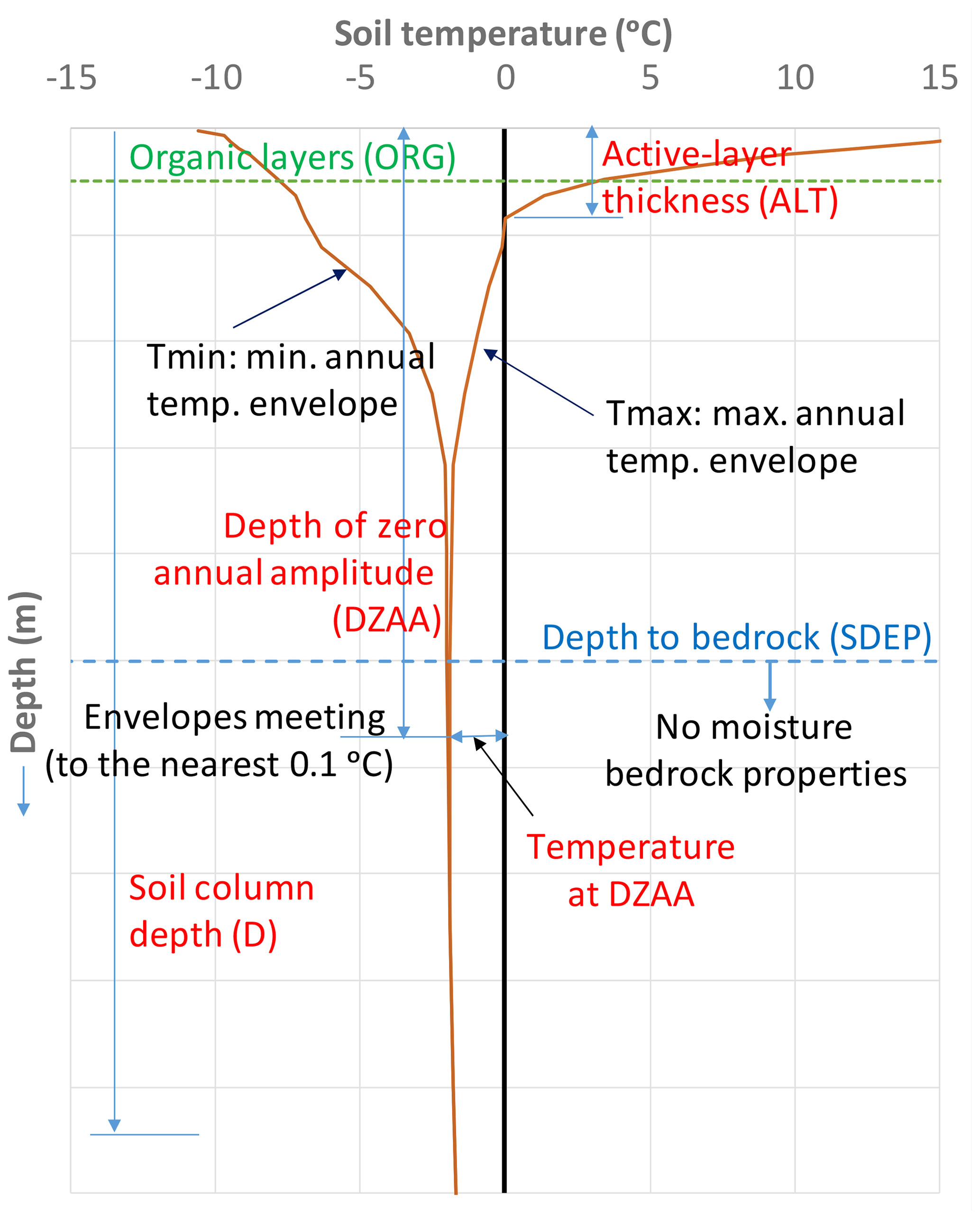
Underground, CLASS couples the moisture and energy balances for a user-specified number of soil layers of user-specified thicknesses, which are uniform across the domain. Each soil layer, thus, has a diagnosed temperature and both liquid and frozen moisture contents down to the soil permeable depth (SDEP) or the “depth to bedrock” below which there is no moisture and the thermal properties of the soil are assumed to be as those of bedrock material (sandstone). MESH usually runs at a 30 min time step, and thus from the MESH-simulated continuous temperature profiles, one can determine several permafrost related aspects that are used in the presented analyses such as (see Fig. 1):
-
Temperature envelopes (Tmax and Tmin) are taken at daily, monthly, and annual time steps and defined by the maximum and minimum simulated temperature for each layer over the specified time period. To compare with available observations, we use the annual envelopes.
-
Active-layer thickness is defined as the maximum depth, measured from the ground surface, of the zero isotherm over the year taken from the annual maximum temperature envelopes by linear interpolation between layers bracketing the zero value (the freezing point depression is not considered) and has to be connected to the surface. The daily progression of ALT can also be generated to visualize the thaw and freeze fronts and determine the dates of thaw and freeze-up. These are calculated in a similar way to the annual ALT but using daily envelopes.
-
Depth of the zero annual amplitude (DZAA) is where the annual temperature envelopes meet within 0.1∘ (van Everdingen, 2005), and the temperature at this depth is TZAA.
Permafrost is usually defined as ground that remains cryotic (i.e. temperature ≤0∘C) for at least 2 years (Dobinski, 2011; van Everdingen, 2005), but for modelling purposes and to validate against annual ground temperature envelopes and ALT observations, a 1-year cycle is adopted. This is common amongst the climate and land surface modelling community (e.g. Park et al., 2013). van Everdingen (2005) defined the active-layer thickness as the thickness of the layer that is subject to annual thawing and freezing in areas underlain by permafrost. Strictly speaking, the active-layer thickness should be the lesser of the maximum seasonal frost depth and the maximum seasonal thaw depth (Walvoord and Kurylyk, 2016). The maximum frost depth can be less than the maximum thaw depth, and, in such a case, there is a layer above the permafrost that is warmer than 0 ∘C but is not connected to the surface (a lateral talik). Because active-layer observations are usually based on measuring the maximum thaw depth, we adopted the same (thaw rather than freeze) criterion when calculating ALT in the model.
Prior versions of MESH/CLASS merely outputted temperature profiles. The code has been amended to calculate the additional permafrost-related outputs detailed above. A typical CLASS configuration consists of 3 soil layers of 0.1, 0.25, and 3.75 m thickness, but in 2006, the CLASS code was amended to accommodate as many layers as needed (Verseghy, 2012). Neglecting lateral heat flow, the one-dimensional finite difference heat conservation equation is applied to each layer to obtain the change in average layer temperature over a time step Δt as
where t denotes the time, i is the layer index, Gi−1 and Gi are the downward heat flux at the top and bottom of the soil layer, respectively, Δzi is the thickness of the layer, Ci is the volumetric heat capacity, and Si is a correction term applied when the water phase changes (freezing or thawing) or the water percolates (exits the soil column at the lowest boundary). The volumetric heat capacity of the layer is calculated as the sum of the heat capacities, Cj, of its constituents (liquid water, ice, soil minerals, and organic matter), weighted by their volume fractions θj and, therefore, varies with time depending on the moisture content.
Heat fluxes between soil layers are calculated using the layer temperatures at each time step using the one-dimensional heat conduction equation
where λ(z) is the thermal conductivity of the soil calculated analogously to the heat capacity. Temperature variation within each soil layer is assumed to follow a quadratic function of depth (z). Setting the flux at the bottom boundary to a constant (i.e. Neumann-type boundary condition for the differential equation) and diagnosing the flux into the ground surface, G(0), from the solution of the surface energy balance results in a linear equation for G(0) as a function of for the different layers in addition to soil surface temperature, T(0). This enables the diagnosing of fluxes and temperatures of all layers using a forward explicit scheme. More details are given in Sect. S1 of the Supplement, and full details are given in Verseghy (2012, 1991).
The CLASS thermal boundary condition at the bottom of the soil column is either “no flux” (i.e. the gradient of the temperature profile should be zero) or a constant geothermal flux. For this study, we considered the no-flux condition, as data for the geothermal flux are not easy to find at the Mackenzie River basin scale. Nicolsky et al. (2007) ignored the geothermal flux in their study over Alaska using CLM with an 80 m soil column. Sapriza-Azuri et al. (2018) showed that the difference in temperature at DZAA between the two cases is within the error margin for geothermal temperature measurements for 60 % of their simulations at Norman Wells. However, we also tested with a constant geothermal flux to verify those previous findings.
As for organic soils, CLASS can use a percentage of organic matter within a mineral soil layer, a fully organic layer, or thermal and hydraulic properties provided directly. As the latter are not usually available, especially at large scales, we used the first two options. In the first case, the organic content is used to modify soil hydraulic and thermal properties, similar to CLM (Oleson et al., 2013). For fully organic soils, CLASS has special values for those properties depending on the type of organic soil selected (fibric, hemic, or sapric) based on the work of Letts et al. (2000) for peat soils (see Sect. S1). In traditional CLASS applications, when the flag for organic soil is activated, fibric (type 1) parameters are assigned to the first soil layer, hemic (type 2) parameters to the second, and sapric (type 3) parameters to deeper layers (Verseghy, 2012; see Supplement Table S1 for parameter values). The corresponding code in MESH was amended such that more than one fibric or hemic layer can be present, and that the organic soil flag can be switched off (returning to a mineral soil parameterization) for lower layers. In assigning the organic-layer type, the same order is used (fibric at the surface, followed by hemic, then sapric with depth), as this represents the natural decomposition process. But with the introduction of many more layers with depth, it is necessary to have more flexibility in how the organic layers can be configured. The fully organic parameterization was activated when the organic content is 30 % or more, based on recommendation by the Soil Classification Working Group (1998).
2.2 Study sites and permafrost data
The Mackenzie River basin extends between 102–140∘ W and 52–69∘ N (Fig. 2). It drains an area of about 1.775×10⁶ km2 of western and northwestern Canada and covers parts of the provinces of Saskatchewan, Alberta, and British Colombia, as well as the Yukon and the Northwest Territories (NWT). The average annual discharge at the basin outlet to the Beaufort Sea exceeds 300 km3, which is the fifth largest discharge to the Arctic. Such a large discharge influences regional as well as global circulation patterns under the current climate, and it is expected to have implications for climate change. Figure 2 also shows the permafrost extent and categories for the MRB taken from the Canadian Permafrost Map (Hegginbottom et al., 1995). About 75 % of the basin is underlain by permafrost that can be either continuous (in the far north and the western mountains), discontinuous (to the south of the continuous region), sporadic (in the southern parts of the Liard and in the Hay sub-basin), or patchy further south. It is important to properly represent permafrost for the MRB model, given the current trends of thawing and its major impacts on landforms and connectivity, and thus the hydrology of the basin. This is achieved through detailed studies conducted at three sites along a transect near the Mackenzie River going from the sporadic permafrost zone (Jean Marie River) to the extensive discontinuous zone (Norman Wells) and the extensive continuous zone (Havikpak Creek) as shown in Fig. 3. The following paragraphs give brief descriptions of the three sites. Table 1 gives details of permafrost monitoring at the sites, while more detailed descriptions are given in Sect. S2 of the Supplement.
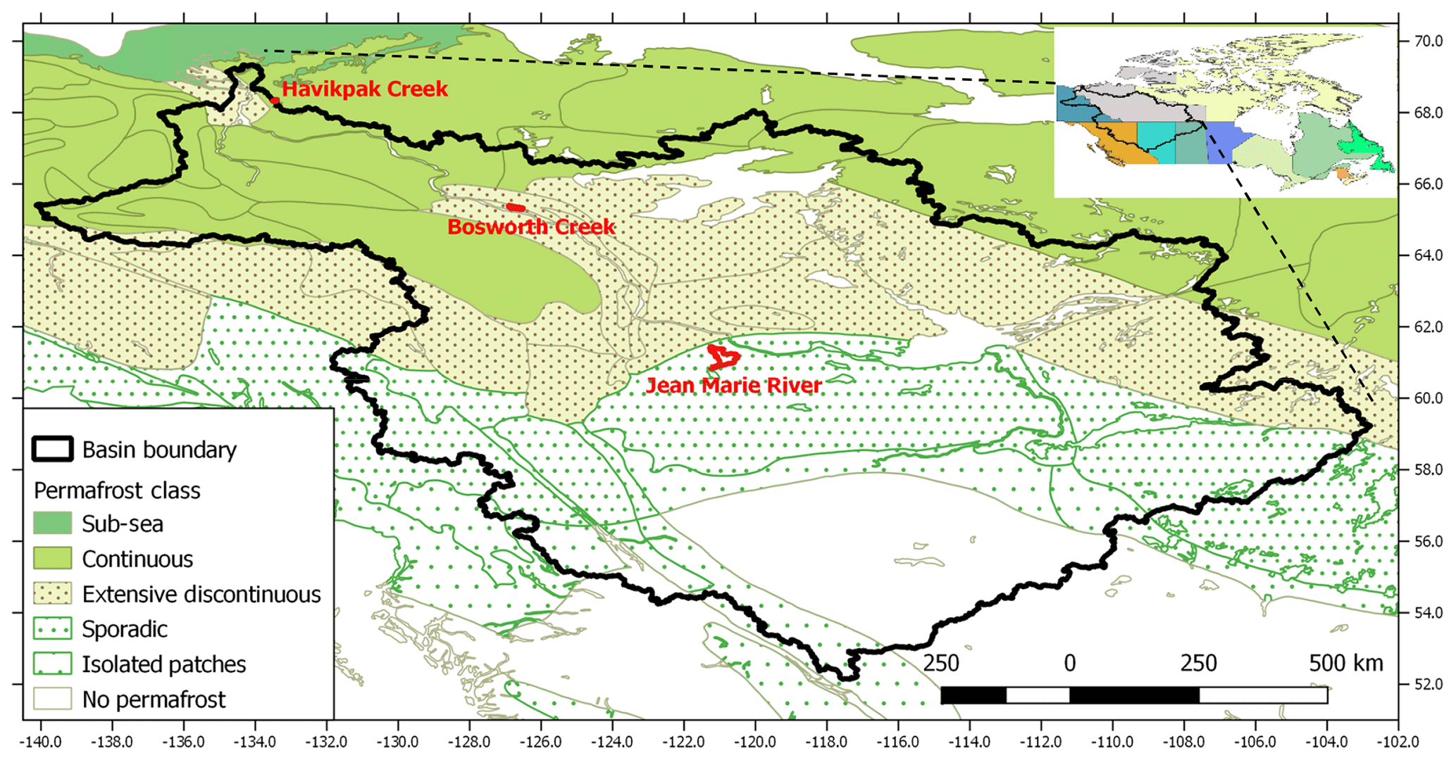
Figure 2Mackenzie River basin: location, permafrost classification, and the three study sites.

Figure 3Location of and permafrost measurement sites in the (a) Jean Marie River sub-basin, (b) Bosworth Creek sub-basin, and (c) Havikpak Creek sub-basin.
Table 1Permafrost sites and important measurements for the study sites. NA: not available. KP: kilometre post (distance from the start of the pipeline in Norman Wells). R.O.W.: right-of-way (of the pipeline).
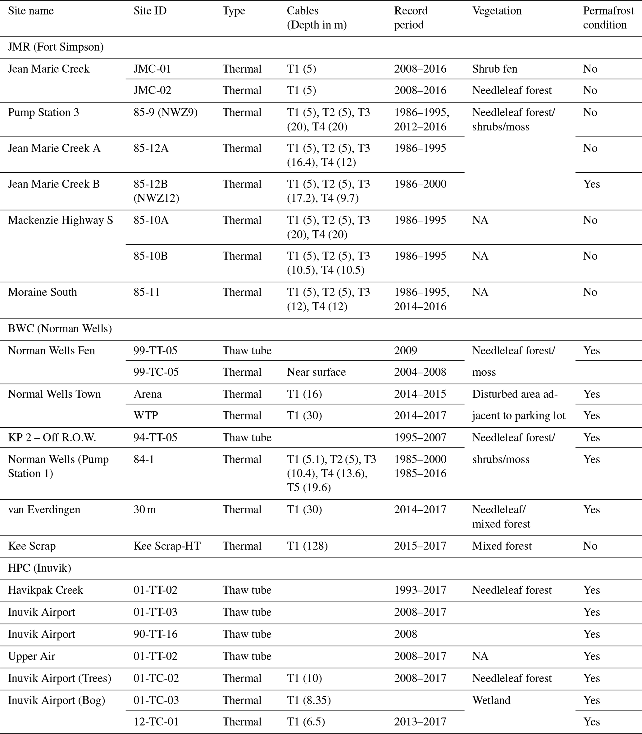
The Jean Marie River (JMR) is a tributary of the main Mackenzie River basin (Fig. 3a) in the Northwest Territories of Canada. The basin is dominated by boreal (deciduous, coniferous, and mixed) forest on raised peat plateaux and bogs. The basin is located in the sporadic permafrost zone where permafrost underlies few spots only and is characterized by warm temperatures ( ∘C) and limited (<10 m) thickness (Smith and Burgess, 2002). The basin and adjacent basins (e.g. Scotty Creek) have been subject to extensive studies because the warm, thin, and sporadic permafrost underling the region has been rapidly degrading (Calmels et al., 2015; Quinton et al., 2011). Several permafrost monitoring sites have been established in and around the basin mostly as part of the Norman Wells–Zama pipeline monitoring program launched by the government of Canada and Enbridge Pipeline Inc. in 1984–1985 (Smith et al., 2004) to investigate the pipeline impact on permafrost conditions. This study uses data from sites 85-12A and 85-12B (see Table 1). Site 85-12A has no permafrost, while site 85-12B, in close proximity, has a thin (3–4 m) permafrost layer with an ALT of about 1.5 m as estimated from soil temperature envelopes over the period 1986–2000. See Fig. S1 in the Supplement for a plot of observed temperature envelopes.
Bosworth Creek (BWC) has a small basin draining from the northeast to the main Mackenzie River near Norman Wells (Fig. 3b). Permafrost monitoring activities started in the region in 1984 with the construction of the Norman Wells–Zama buried oil pipeline (as described above). The basin is dominated by boreal (deciduous, coniferous, and mixed) forest. It is located in the extensive discontinuous permafrost zone with relatively deep active-layer (1–3 m) and relatively thick (10–50 m) permafrost (Smith and Burgess, 2002). Sapriza-Azuri et al. (2018) used cable T5 at the Pump Station 1 site (84-1) (see Table 1) to investigate the appropriate soil depth and initial conditions for their permafrost simulations, which serve as a pre-cursor for this current study. They recommended a soil depth of at least 20 m to ensure that the simulated DZAA is within the soil profile. However, they based their analysis on cable T5, which is within the right-of-way of the pipeline and is likely to be affected by its construction or operation. We focus on the Norman Wells Pump Station 1 site (84-1), and for this study we choose cable T4 as it is more likely to reflect the natural permafrost conditions being out of the right of way of the pipeline. There has been a continuous record since 1985 (Smith et al., 2004; Caroline Duchesne, personal communication, 2017).
Havikpak Creek (HPC) is a small Arctic research basin (Fig. 3c) located in the eastern part of the Mackenzie River basin delta, 2 km north of Inuvik Airport in the Northwest Territories. The basin is dominated by sparse taiga forest and shrubs and is underlain by thick permafrost (>300 m). The basin has been subject to several hydrological studies, especially during the Mackenzie GEWEX (Global Energy and Water Exchanges) Study (MAGS). Recently, Krogh et al. (2017) modelled its hydrological and permafrost conditions using the Cold Regional Hydrological Model (CRHM) (Pomeroy et al., 2007). They integrated a ground freeze and thaw algorithm called XG (Changwei and Gough, 2013) within CRHM to simulate the active-layer thickness and the progression of the freeze and thaw front with time, but they did not attempt to simulate the temperature envelopes or DZAA. Ground temperatures are measured with temperature cables installed in boreholes at two sites, 01TC02 and 01TC03, respectively (Smith et al., 2016). In addition, there are three thaw tubes at the Inuvik Upper Air station (90-TT-16) just to the west of the basin, at HPC proper (93-TT-02), and at the Inuvik Airport (Bog) site (01-TT-03) measuring the active-layer depth and ground settlement (Smith et al., 2009).
2.3 Land cover parameterization
Parameterizations for the three selected basins were extracted from a larger MRB model, described in Elshamy et al. (2020). This includes the land cover characterization and parameters for vegetation and hydrology. The land cover data are based on the Canada Centre for Remote Sensing (CCRS) 2005 dataset (Canada Centre for Remote Sensing et al., 2010). The parameterization of certain land cover types differentiates between the eastern and western sides of the basin using the Mackenzie River as a divide, informed by calibrations of the MRB model. HPC and BWC are on the east side of the river, while JMR is on the west side, and therefore these setups have different parameter values for certain GRU types (e.g. needleleaf forest). SDEP, soil texture information, and initial conditions were taken as described above and adjusted according to model evaluation versus permafrost-related observations (ALT, DZAA, and temperature envelopes) with the aim of developing an initialization and configuration strategy that can be implemented for the larger MRB model.
Provisions for special land covers within the MESH framework include inland water. Because of limitations in the current model framework, inland water must be represented as a porous soil. This is parameterized such that it remains as saturated as possible, drainage is prohibited from the bottom of the soil column, and it is modelled using CLASS with a large hydraulic conductivity value and no slope. Additionally, it was initialized to have a positive bottom temperature, and therefore, it does not develop permafrost. Wetlands are treated in a similar way (impeded drainage and no slope) but with grassy vegetation and preserving the soil parameterization as described in below in Sect. 2.5 and 2.6. It remains close to saturation but can still be underlain by permafrost, depending on location. Taliks are allowed to develop under wetlands this way.
2.4 Climate forcing
MESH requires seven climatic variables at a sub-daily time step to drive CLASS. For this study we used the WFDEI (WATer and global CHange (WATCH) Forcing Data (WFD) with the ERA-Interim analysis from the European Centre for Medium-Range Weather Forecasts) dataset that covers the period 1979–2016 at 3-hourly resolution (Weedon et al., 2014). The dataset was linearly interpolated from its original resolution to the MRB model grid resolution of . The high resolution forecasts of the Global Environmental Multiscale (GEM) atmospheric model (Côté et al., 1998b, a; Yeh et al., 2002) and the Canadian Precipitation Analysis (CaPA; Mahfouf et al., 2007) datasets, often combined as GEM-CaPA, provide the most accurate gridded climatic dataset for Canada in general (Wong et al., 2017). Unfortunately, these datasets are not available prior to 2002 when most of the permafrost observations used for model evaluation are available. However, an analysis by Wong et al. (2017) showed that precipitation estimates from the CaPA and WFDEI products are in reasonable agreement with station observations. Alternative datasets such as WFD (Weedon et al., 2011) and Princeton (Sheffield et al., 2006) go earlier in time (1901) but are not being updated (WFD stops in 2001, while Princeton stops in 2012). Additionally, Wong et al. (2017) showed that the Princeton dataset has large precipitation biases for many parts of Canada. Analysis of the sensitivity of the results presented here regarding the choice of the climatic dataset is beyond the scope of this work.
2.5 Soil profile and permeable depth
As mentioned earlier, Sapriza-Azuri et al. (2018) recommended a total soil column depth (D) of no less than 20 m to enable reliable simulation of permafrost dynamics considering the uncertainties involved mainly due to parameters. Their study is relevant because they used the same model used in this study (MESH/CLASS). They studied several profiles, down to 71.6 m depth. Recent applications of other H-LSMs also considered deep soil column depths; e.g. CLM 4.5 used 42.1 m (Oleson et al., 2013), and CHANGE (Park et al., 2013) used 30.5 m. After a few test trials with D=20, 25, 30, 40, 50 and 100 m at the study sites, we found that the additional computation time when adding more layers to increase D is outweighed by the reliability of the simulations. The reliability criterion used here is that the temperature envelopes meet (i.e. DZAA) well within the soil column depth over the simulation period (including spin-up) such that the bottom boundary condition does not disturb the simulated temperature profiles and envelopes and ALT (Nicolsky et al., 2007). DZAA is a relatively stable indicator for this criterion (Alexeev et al., 2007). The simulated DZAA reached a maximum of 20 m at one of the sites in a few years, and thus a total depth of 50 m was used in anticipation for possible changes in DZAA with future warming. We show that this depth is adequate at the three sites selected in the subsequent sections.
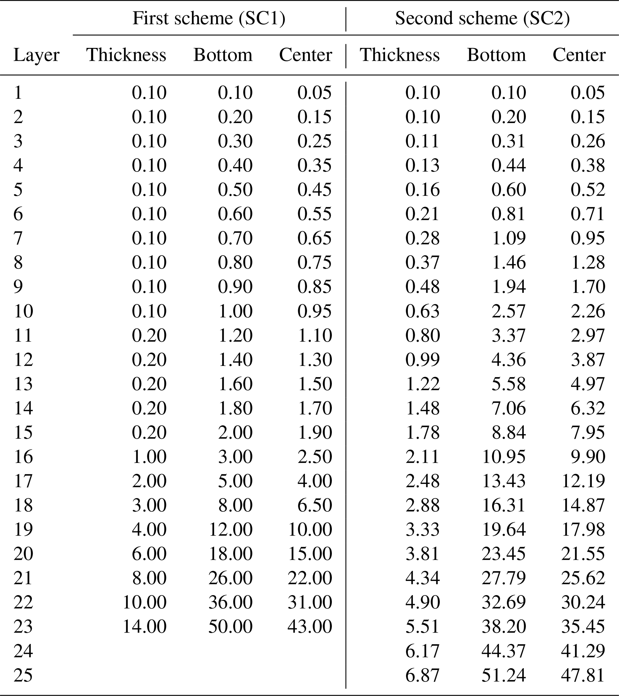
As noted above, the total soil column depth is only one factor in the configuration of the soil. The layering is as critical. In former modelling studies, exponentially increasing soil layer thicknesses were used, aiming to reach the required depth with a minimum number of layers. The exponential formulation creates more layers near the surface, which allows the models to capture the strong soil moisture and temperature gradients there and yet have a reasonable number of layers (15–20) to reduce the computational burden. However, for most of the MRB, the observed ALT is in the range of 1–2 m from the surface, and the exponential formulations increase layer thickness quickly after the first 0.5–1.0 m, which reduces the accuracy of the model, especially for transient simulations. Therefore, we adopted two layering schemes that have more layers in the top 2 m and increased layer thicknesses at lower depths to a total depth near 50 m. The first scheme has the first metre divided into 10 layers, the second metre divided into 5 layers, and the total soil column has 23 layers. The second scheme has soil thicknesses increasing more gradually to reach 51.24 m in 25 layers following a scaled power law. This latter scheme has the advantage that each layer is always thicker than the one above it (except the second layer), as the explicit forward difference numerical scheme to solve the energy and water balances in CLASS can have instabilities when layers in succession have the same thickness. The minimum soil layer thickness is taken as 10 cm as advised by Verseghy (2012). Table 2 shows the soil layer thicknesses and centers (used for plotting temperature profiles and envelopes) for both soil layering schemes.
As mentioned before, the permeable depth marks the hydrologically active horizon below which the soil is not permeable and where its thermal properties are changed to those of bedrock material. This makes it an important parameter for not only for water storage but also for thermal conductance. It was set for the various study basins from the Shangguan et al. (2017) dataset interpolated to 0.125∘ and the MRB model grid resolution by Keshav et al. (2019b). The sensitivity of the results to SDEP is assessed by perturbing it within a reasonable range at each site as shown in the results.
2.6 Configuration of organic soil
Organic soils were mapped from the Soil Landscapes of Canada (SLC) v2.2 dataset (Centre for Land and Biological Resources Research, 1996) for the whole MRB (Fig. 4) at 0.125∘ resolution by Keshav et al. (2019a). However, this dataset does not provide information on the depth of the organic layers or their configuration (i.e. the thicknesses of fibric, hemic, and sapric layers in peaty soils). Therefore, different configurations have been tested at the study sites based on available local information (Table 3). We also compared fully organic configurations (ORG) at the three sites with mineral configurations with organic content (M-org) to investigate the appropriate configuration at each site, keeping in mind the need to generalize it for larger basins.
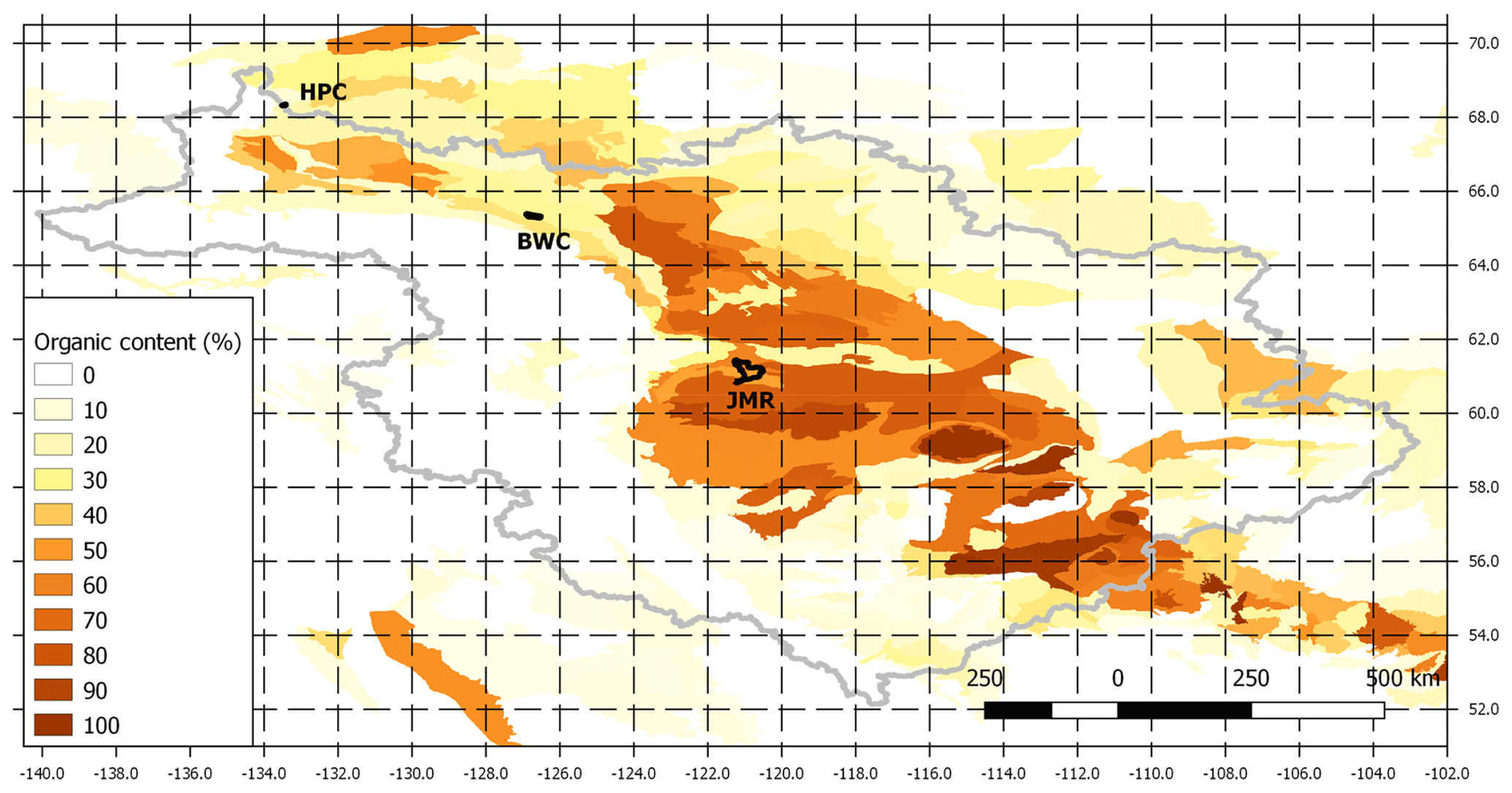
Figure 4Gridded organic matter in soil at 0.125∘ resolution for the MRB, processed from the Soil Landscapes of Canada (SLC) v2.2 dataset (Centre for Land and Biological Resources Research, 1996).
Table 3The number of layers of each organic sub-type for fully organic soil configurations (ORG) and organic content for mineral configurations (M-org).
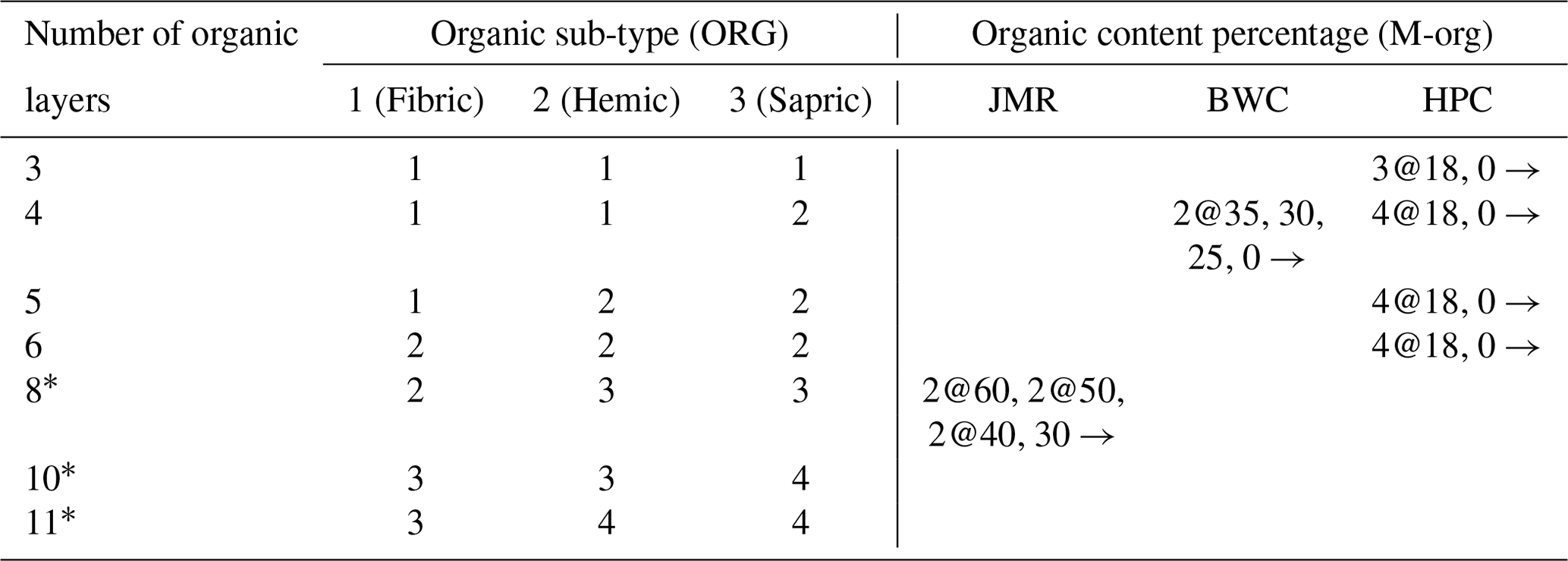
∗ Only used for JMR; x@y means x layers with the specified percentage, and x→ means the value is for the remainder of the layers below.
For JMR, we tested configurations with about 0.3 m organic soil (three layers) to over 2 m of organic soil, where organic content from SLC v2.2 ranged between 48 %–59 % (Fig. 4). The soil texture immediately below these layers was characterized as a mineral soil of uniform texture with 15 % sand and 15 % clay content, with the remainder assigned as silt. Peat depths of 4–7 m in the surrounding region have been identified in reports (Quinton et al., 2011) and by borehole data at permafrost monitoring sites (Smith et al., 2004). Therefore, layers at these depths until bedrock were characterized as mineral soils (as described above), but they had 50 % organic content. These deeper layers, while having considerable organic content, do not use the previously described parameterization for fully organic soils. This is an exception for this basin, which could be generalized for the MRB in areas with high organic content (e.g. >50 %) like this region. These configurations are summarized in Table 3. For the M-org configuration, we used a decreasing organic content with depth.
For BWC, the organic map indicated that organic matter ranges between 27 %–34 %. We tested configurations with 0.3–0.8 m organic layers. A borehole log for the 84-1-T4 site (Smith et al., 2004) shows a thin organic silty layer at the top (close to 0.2–0.3 m). Sand and clay content below the organic layers are uniformly taken to be 24 % and 24 % respectively based again on SLC v2.2, with the remainder (52 %) assumed to be silt. We tested ORG and M-org configurations as shown in Table 3.
The organic content indicated by the gridded soil information at HPC is only 18 %, which is lower than the 30 % threshold decided for fully organic soils. However, Quinton and Marsh (1999) used a 0.5 m thick organic layer in their conceptual framework developed to characterize runoff generation in the nearby Siksik Creek. Krogh et al. (2017) adopted the same depth for their modelling study of HPC. Therefore, we tested configurations with 0.3–0.8 m fully organic layers as well as the M-org configuration with a uniform 18 % organic content. Below that, soil texture values are taken to be 24 % sand and 32 % clay from SLC v2.2.
2.7 Spin-up and stabilization
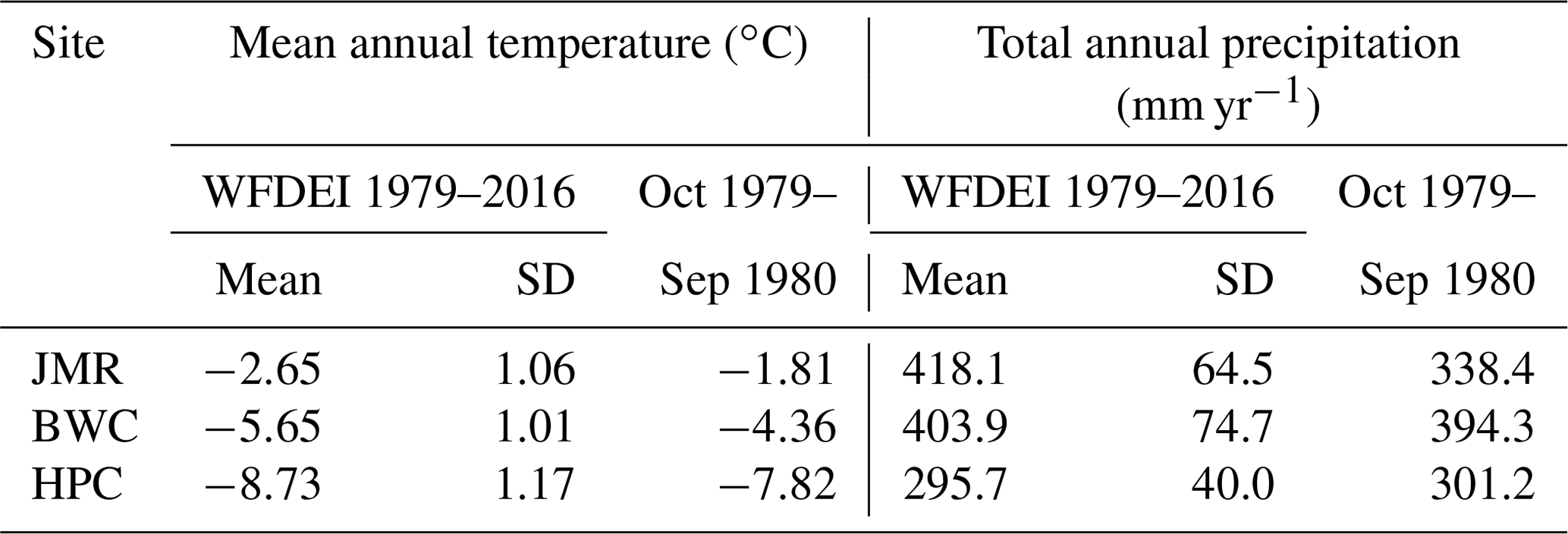
We used the first hydrological year of the climate forcing (October 1979–September 1980) to spin up the model repeatedly for 2000 cycles while monitoring the temperature and moisture (water and ice contents) profiles at the end of each cycle for stabilization. We checked that the selected year was close to average in terms of temperature and precipitation compared to the WFDEI record (1979–2016) as shown in Table 4. The start of the hydrological year was selected because it is easier to initialize CLASS when there is no snow cover or frozen soil moisture content. Stabilization is assessed visually using various plots as well as by computing the difference between each cycle and the previous one making sure the absolute difference does not exceed 0.1 ∘C for temperature (which is the accuracy of measurement of the temperature sensors) and 0.01 m3 m−3 for moisture components for all soil layers. The aim is to determine the minimum number of cycles that could inform the ongoing development of the MRB model, as it is computationally very expensive to spin up the whole MRB domain for 2000 cycles. We then assessed the impact of running the model for the period 1980–2016 after 50, 100, 200, 500, 1000, and 2000 spin-up cycles on ALT, DZAA, and the temperature envelopes at the three sites for selected years depending on the available observations. We assessed the quality of the simulations visually as well as quantitatively by calculating the root mean squared error (RMSE) for ALT, DZAA, and the temperature profiles.
Table 4Comparison of temperature and precipitation of the selected spinning year to mean climate of the WFDEI Dataset.
3.1 Establishing initial conditions
Figure 5 shows the temperature profiles at the end of spinning cycles for a selected GRU (needleleaf forest; NL) for the three selected sites using the two suggested soil layering schemes (SC1 and SC2) and using two different organic configuration (ORG and M-org) for SC2. NL forest is representative of the vegetation at the selected thermal sites for the three studied basins (except the HPC bog site). As expected, the profile changes quickly for the first few cycles then tends to stabilize such that no significant change occurs after 100 cycles and less in most cases. Similar observations can be made for soil moisture (both water and ice contents) from Fig. 6. Changes in moisture content tend to diminish more quickly than those for temperature, especially for ORG, and thus we will focus on temperature changes in the remaining results. However, water and ice fractions play important roles in defining the thermal properties of the soil and provide useful insights to understand certain behaviours in the simulations. Figure 7 shows the temperature of each layer for the same cases versus the cycle number to visualize the patterns of change over the cycles. Small oscillations are observed, indicating minor numerical instabilities in the model, but these do not cause major differences for the simulations. In some cases, the temperature keeps drifting for several hundred cycles before stabilizing (if stabilization occurs). We note a few important findings:
-
The temperature of the bottom layer (TBOT) remains virtually unchanged from its initial value. This triggered further testing using different initial values, and the impacts on stabilization were similar, as shown in the next sections. We also checked the model behaviour for shallower soil columns and found that the bottom temperature did change during spin-up, within a range that decreased as the total soil depth increased.
-
The vertical discretization of the soil plays an important role in the evolution of temporal moisture and temperature profiles. SC2 results in faster stabilization than SC1 with less drifting for all cases.
-
The depth of organic layers, and their sub-type in fully organic soils, controls the shape of the moisture content profiles and the ice and water content partitioning. This in turn influences the soil thermal properties (drier soils are generally less conductive, and icy soils are more conductive) and thus affects the number of cycles needed to reach stable conditions. Deeper fully organic soils (JMR) require more cycles to stabilize than mineral ones with organic content.
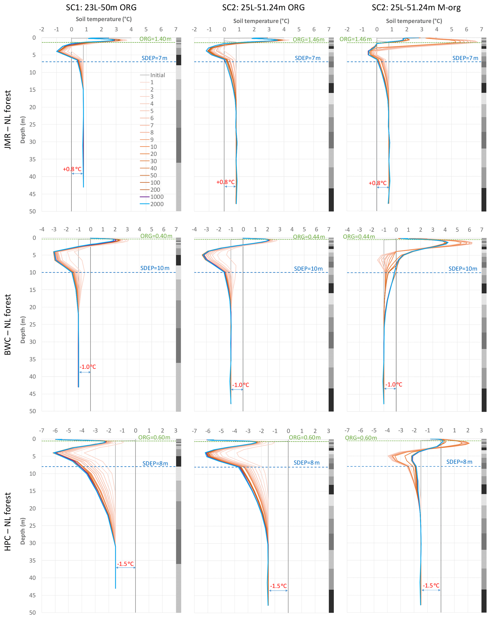
Figure 5Soil temperature profiles at the end of selected spin-up cycles for the NL forest GRU at all three sites using different soil layering schemes and organic configurations; grey bars on the side indicate soil layers.
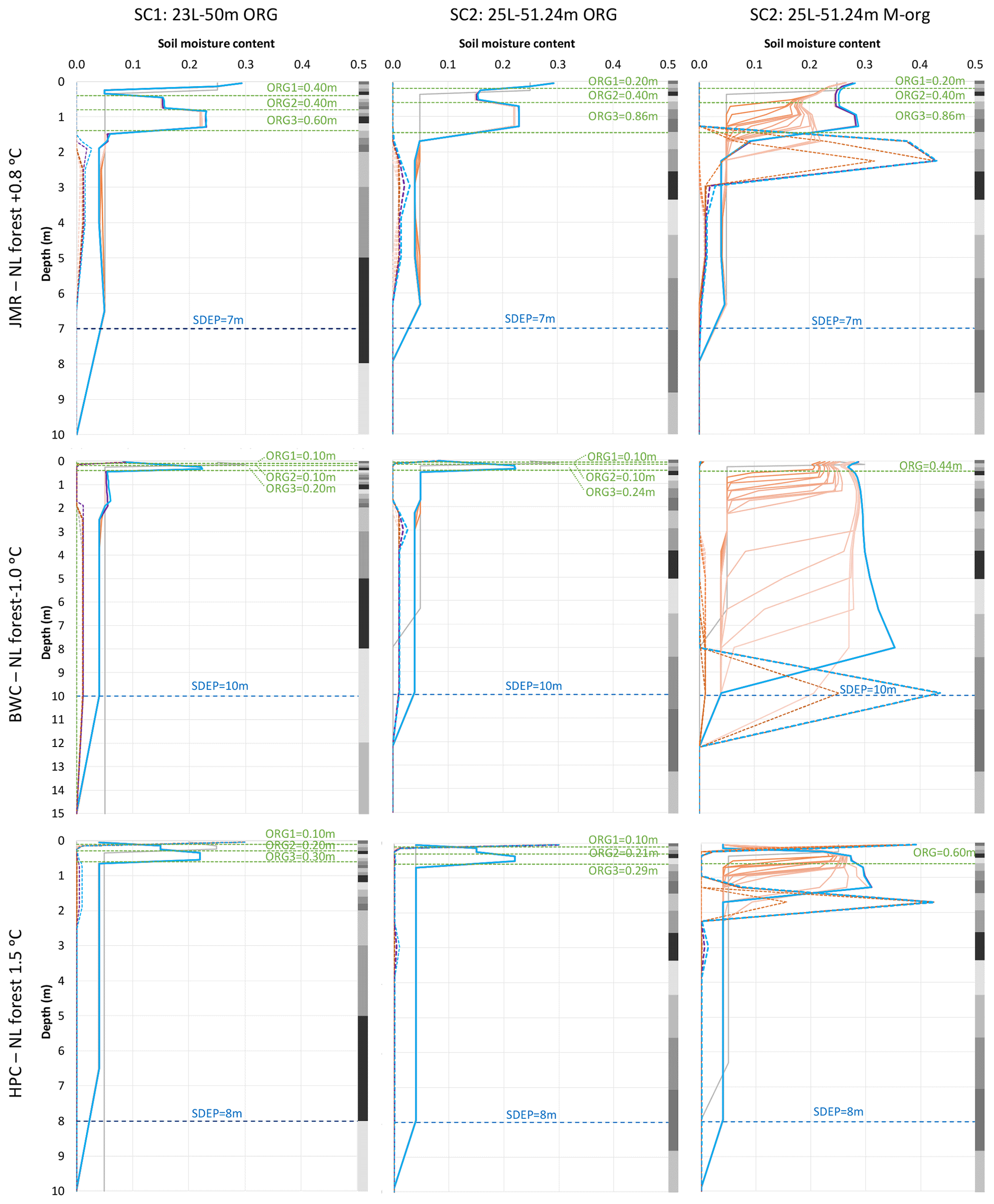
Figure 6Soil moisture profiles at the end of selected spin-up cycles for the NL forest GRU at all three sites using different soil layering schemes and organic configurations. Solid lines indicate liquid, and dashed lines indicate ice. Grey bars on the side indicate soil layers. The legend is as in Fig. 5.
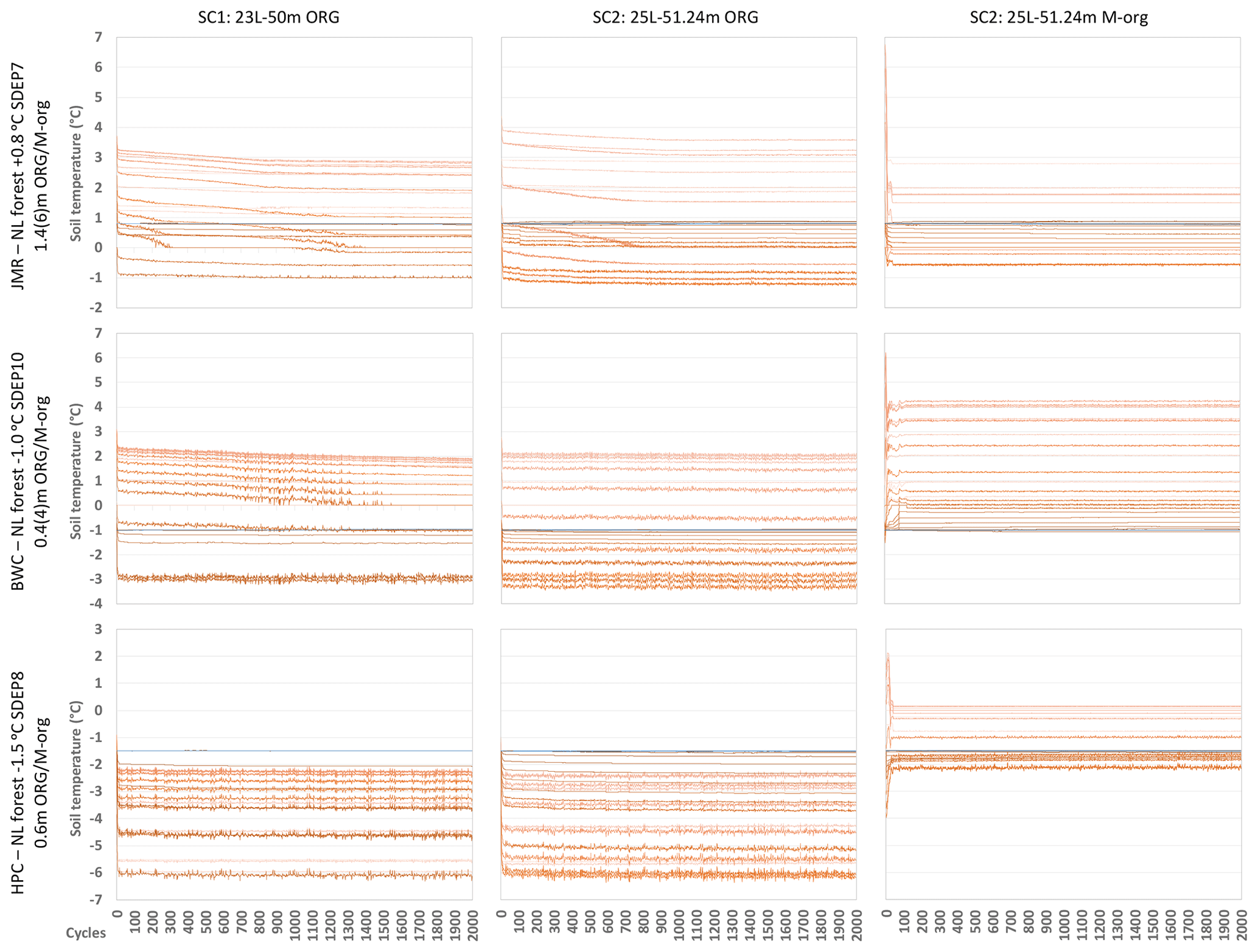
Figure 7Impact of the soil layering scheme selection on spin-up convergence at the three study sites (the darker the colour, the deeper the layer; the deepest layer is coloured blue).
The temperature gradient northward is clear comparing the different sites as well as the impact of the deeper organic layers at JMR on the slower stabilization of temperature and, to a lesser extent, moisture content. This is related to the low thermal conductivity of organic matter as well as the low moisture content below the organic layers as peat acts as a sponge absorbing water and heat and disallowing downward propagation, especially in the absence of ice (i.e. in summer). Hemic and sapric peat soils have relatively high minimum water contents as shown in Fig. 6 (see also Table S1 in the Supplement). The M-org configuration allows more moisture to seep below the organic layers and have some higher ice content at some depth, which depends on the thickness of the organic layers and the general site conditions. For example, it forms below the thick organic layers for JMR, but it formed at a deeper depth at BWC as the organic thickness is smaller. HPC has a comparable organic depth to BWC, but the layers with high ice content formed at a shallower depth because the site is colder. At all three sites, and for both ORG and M-org configurations, there is a change in the slope of the temperature profile at the depth corresponding to the interface of the soil to bedrock, illustrating the importance of the SDEP parameter for permafrost simulations. This is caused by the change in soil thermal properties above and below SDEP (respective of the two different mediums above and below this interface) and the moisture contents therein; bedrock is assumed to remain dry at all times, while soil will always have a minimum liquid water content depending on its type.
Given the above findings, the remainder of the results focus on SC2 only. Additionally, we considered different values for the bottom temperature based on site location and the extrapolation of observed temperature profiles. This is because it cannot be established through spin-up, and ground temperature measurements rarely go deeper than 20 m. There are established strong correlations between near-surface ground temperature and air temperature at the annual scale (e.g. Smith and Burgess, 2000), but the near-surface ground temperature is taken just a few centimetres below the surface. We spin up the model at the three sites for 2000 cycles for a few cases and then use the initial conditions after a selected number of cycles to run a simulation for the period of record (1979–2016) and assess the differences for ALT, DZAA, and the temperature profiles. The sensitivity of the results to SDEP, TBOT, and the organic soil depth will then be assessed using 100 spin cycles only.
3.2 Impact of spin-up
Figures 8, 9, and 10 show the simulated ALT, DZAA and temperature envelopes (selected years) at the three study sites respectively using initial conditions after 50, 100, 200, 500, 1000, and 2000 spin-up cycles using SC2 and the stated configuration for SDEP, TBOT, and ORG and M-org. Most differences across the spin-up range are negligible. What stands out are some large differences in ALT and DZAA at JMR for some years (ORG configuration only) depending on the initial conditions (i.e. number of cycles) used. The low thermal conductivity of the thick fully organic layers slows the stabilization process and thus yields slightly different initial conditions depending on the number of cycles used. That does not happen for the two other sites with thinner ORG layers or for M-org configurations. This is further emphasized by the RMSE values for ALT and DZAA shown in the legends of Figs. 8 and 9.
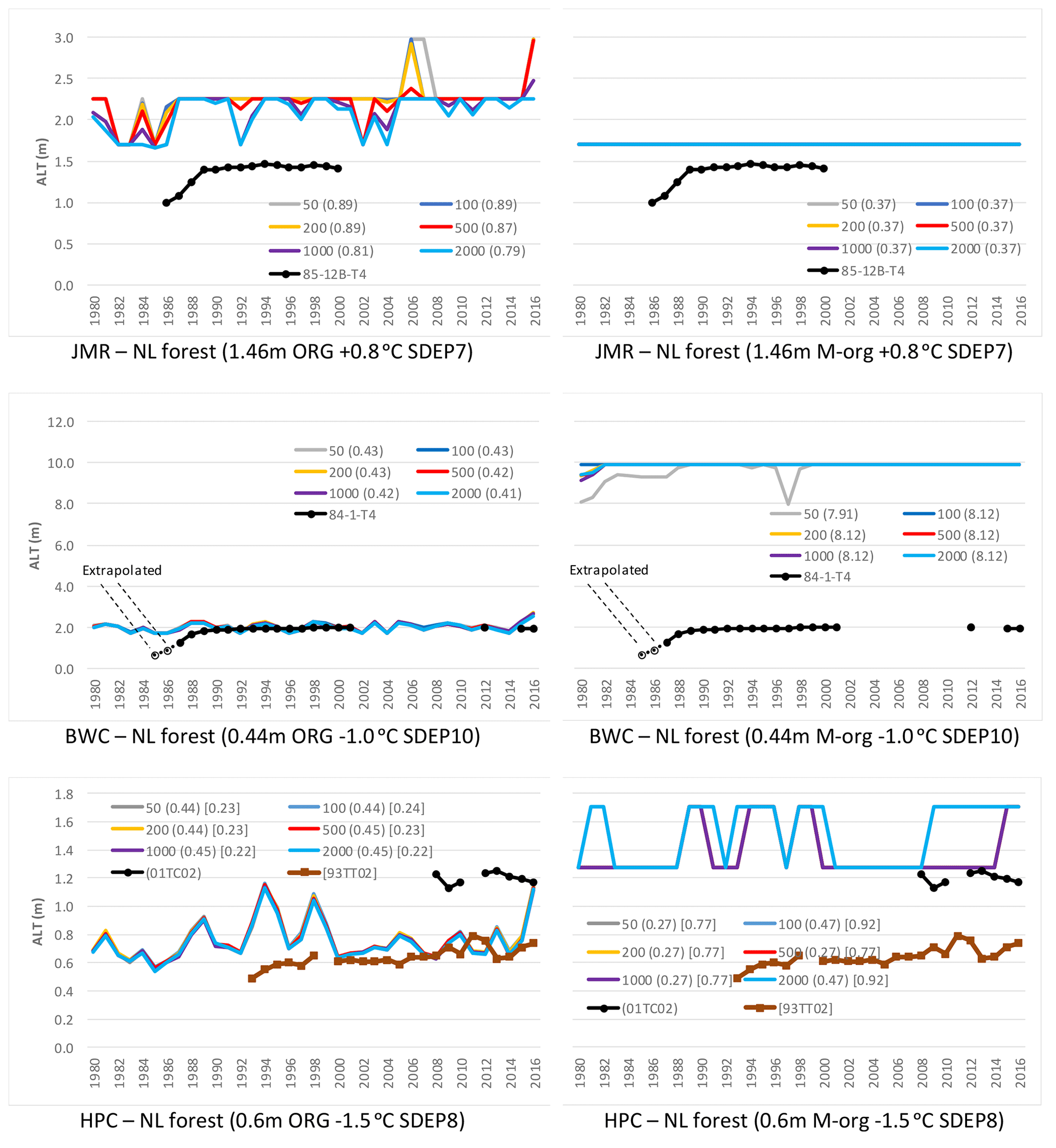
Figure 8Impact of the number of spin-up cycles on the simulated ALT for the needleleaf forest GRU at all sites. Two organic configurations were used for each site using the SC2 layering scheme; RMSE is shown in parenthesis.
Assuming that more spin-up cycles would lead to diminished differences, and thus considering the results initiated after 2000 cycles as a benchmark, one can accept an error of a few centimetres in the simulated ALT using a smaller number of spin-up cycles. For JMR, this error is about 10 % on average, which is much smaller than the error in simulating ALT at this site. Thus, there is a trade-off in computational time by limiting the number of cycles required for a slight loss of accuracy at some sites, particularly those located in the more challenging sporadic zone.
The figures also include relevant observations and RMSE values to assess the quality of simulations. The simulated ALT at JMR are overestimated (Fig. 8) by the ORG configuration. The M-org configuration does better for a mean ALT at JMR but is much worse than ORG for BWC which overestimates ALT by about 8 m. For BWC, the ALT simulation under ORG is close to observations for most years, but the simulation shows more interannual variability, while observations show a small upward trend after an initial period of a large increase (1988–1992), which may be the result of the disturbance of establishing the site. A couple of observations are marked “extrapolated” as the zero isotherm falls above the first thermistor (located 1 m deep). For HPC, M-org better represents the conditions at 01-TC-02, while ORG, resulting in a smaller ALT on average, is closer to the thaw tube measurements at HPC (93-TT-02), as indicated by the RMSE values. This is indicative of the large heterogeneity of conditions that can occur in close proximity to each other and that require different modelling configurations. M-org configurations generally show little to no interannual variability (except for HPC), while ORG ones show more interannual variability.

Figure 9Impact of the number of spin-up cycles on simulated DZAA for the needleleaf forest GRU at all three sites. Two organic configurations were used for each site using the SC2 layering scheme; RMSE is shown in parenthesis.
The simulated DZAA (Fig. 9) is overestimated at JMR under both ORG and M-org configurations, while it is close to values deduced from observations at BWC and HPC. In contrast to ALT, DZAA observations have larger interannual variability than simulations, possibly due to the large spacing of measuring thermistors and the failure of some in some years. For HPC, both ORG and M-org simulations are showing more variability in DZAA than the depth deduced from observations for 01-TC-02, and both underestimate it. In general, matching DZAA to observations is not an objective in itself, but its occurrence well within the selected soil depth is more important. The largest value simulated is about 19 m for HPC, which is less than half the total soil depth. This indicates that a smaller soil column depth would not be suitable for HPC but could be used for JMR and BWC.
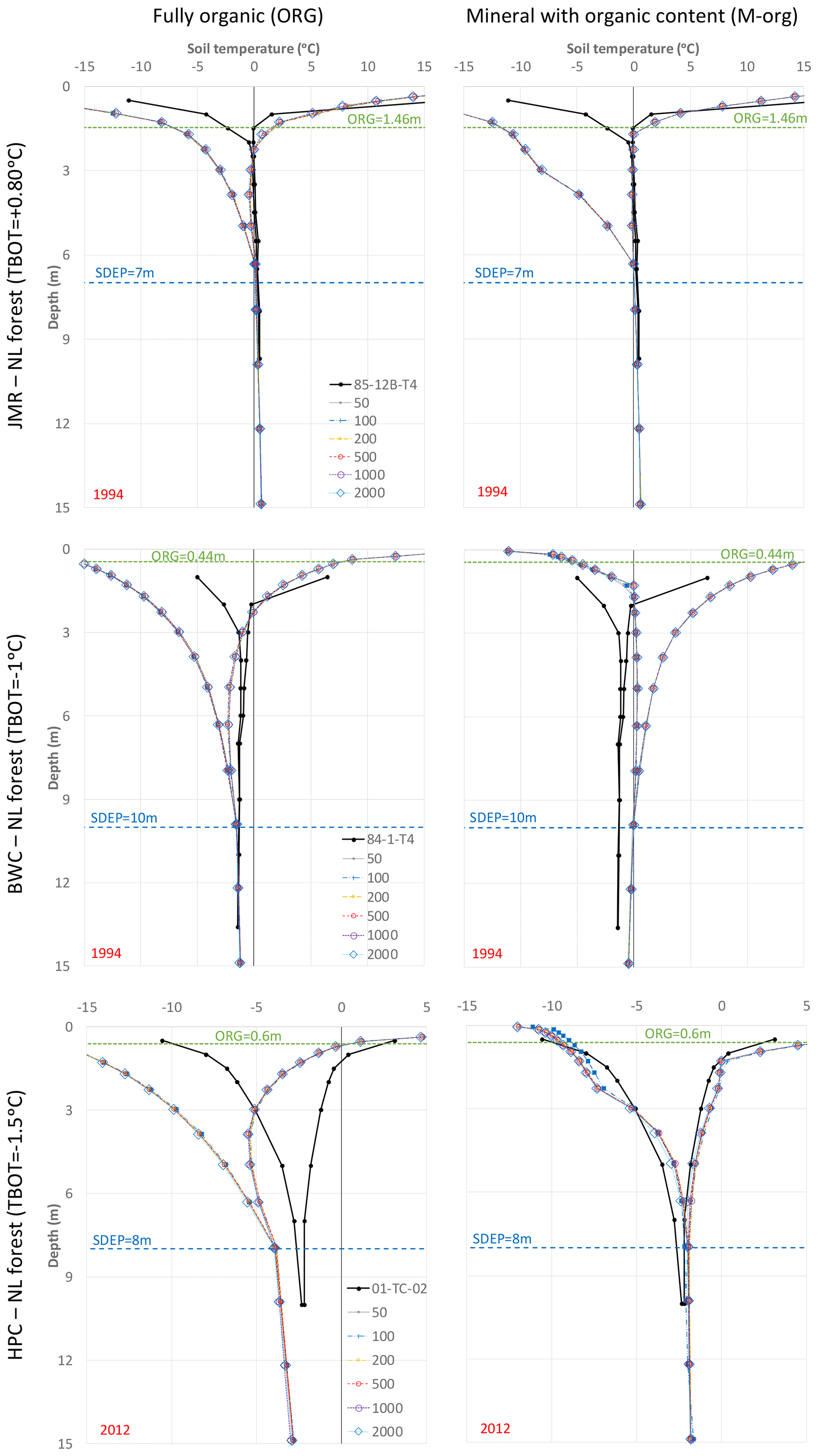
Figure 10Impact of the number of spin-up cycles on simulated temperature envelopes for the needleleaf forest GRU for a selected year at each study site. Two organic configurations were used for each site using the SC2 layering scheme.
Comparing temperature profiles for a selected year at each site (Fig. 10) reveals a large difference between ORG and M-org configurations, especially at HPC and BWC. The overall shapes of the profiles depend on the selected configuration. M-org works better for HPC, while ORG is better at BWC. Both configurations do relatively well for JMR, although this site is characterized with deep peat. At BWC, the ORG simulation agrees well with observations in terms of ALT, but the temperature envelopes are generally colder than observed. The M-org configuration at this site results in a talik between 2 and 9 m which is not seen in the observations. The minimum envelope is too cold near the surface for ORG configurations at the three sites because of the thermal properties of the peat (Dobinski, 2011; Kujala et al., 2008). This is discussed further in Sect. 3.5.
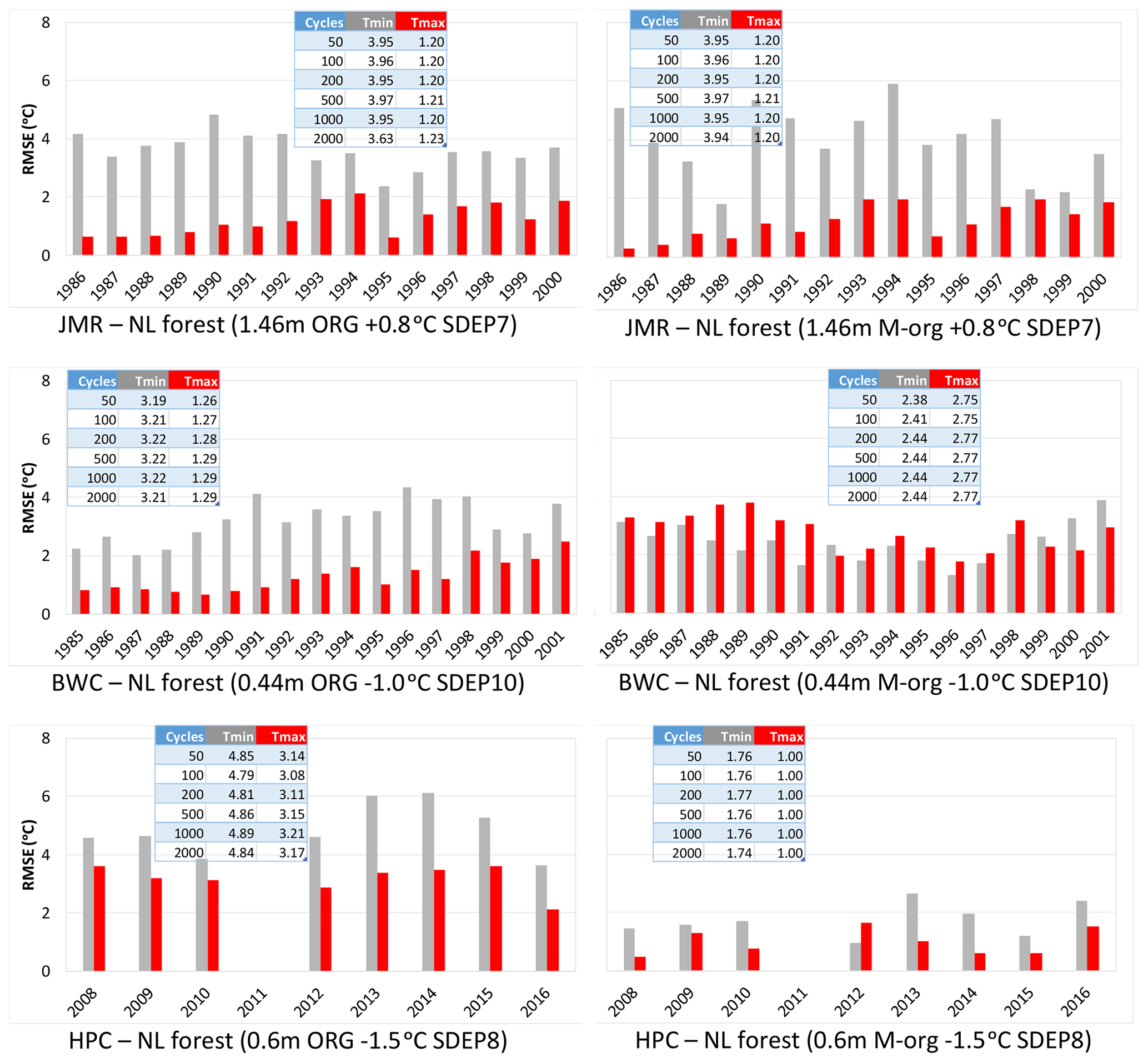
Figure 11Time series of RMSE of simulated envelopes at all three sites at the end of 2000 cycles. Two organic configurations were used for each site using the SC2 layering scheme. Table insets show the change in mean RMSE over the period of the available record for simulations initiated after the number of spin-up cycles.
To aid with the selection of the best configuration for each site, we calculated RMSE for the temperature envelopes (Tmax and Tmin separately) by interpolating the simulation results at the depths of observations, discarding points and years where and when the sensors fail. The available records vary from site to site. The results are shown in Fig. 11 for the simulations that stared after 2000 spin-up cycles with a small inset table on each panel showing how the mean RMSE over the simulation period changes with spin-up cycles. The change in RMSE with cycles is small to negligible. In general, Tmax is better simulated than the Tmin, except for the BWC M-org configuration. M-org has lower errors than ORG for HPC, while the situation is reversed for HPC (i.e. M-org is better than ORG). For JMR, the performance of the ORG configuration is similar to M-org for Tmax, but it is better for Tmin. The shape of the Tmin envelope is better. Given the requirement to have generic rules to be applicable at the MRB scale, we prefer to use the ORG configuration at this site. The following sections assess the sensitivity of the results to SDEP, TBOT, and organic depth for the preferred configuration at each site.
3.3 Impact of permeable depth (SDEP)
SDEP for the above-mentioned configurations for each site was perturbed in the range of 5–15 m keeping other studied parameters (TBOT and organic configuration) fixed. Figure 12 shows the impact for each site on the average ALT and DZAA over the analysis period (1980–2016) for all land cover types. A total of 100 spin-up cycles were used to initialize those simulations. The land-cover-derived GRUs vary between the sites. For JMR, wetlands do not develop permafrost, while at shallower SDEP values, taliks (i.e. no permafrost; NPF) develop under forest GRUs in some years. Thus, the averages shown on Fig. 12 are for those years when the soil is cryotic all year round, which varies across the tested SDEP range. There is a general tendency for ALT to slightly decrease with deeper SDEP values for all land cover types, except for grass and shrubs at HPC. The impact of SDEP on DZAA varies across sites and GRUs. While DZAA increases initially with SDEP at JMR then becomes insensitive, it initially decreases with SDEP for HPC then increases at a slower rate. At BWC it initially decreases with a larger SDEP then increases before becoming insensitive to SDEP. DZAA is generally shallower for JMR followed by BWC and then HPC in close correlation with the depth of organic layers. This behaviour may also be correlated to the thickness of permafrost that increases in the same order.
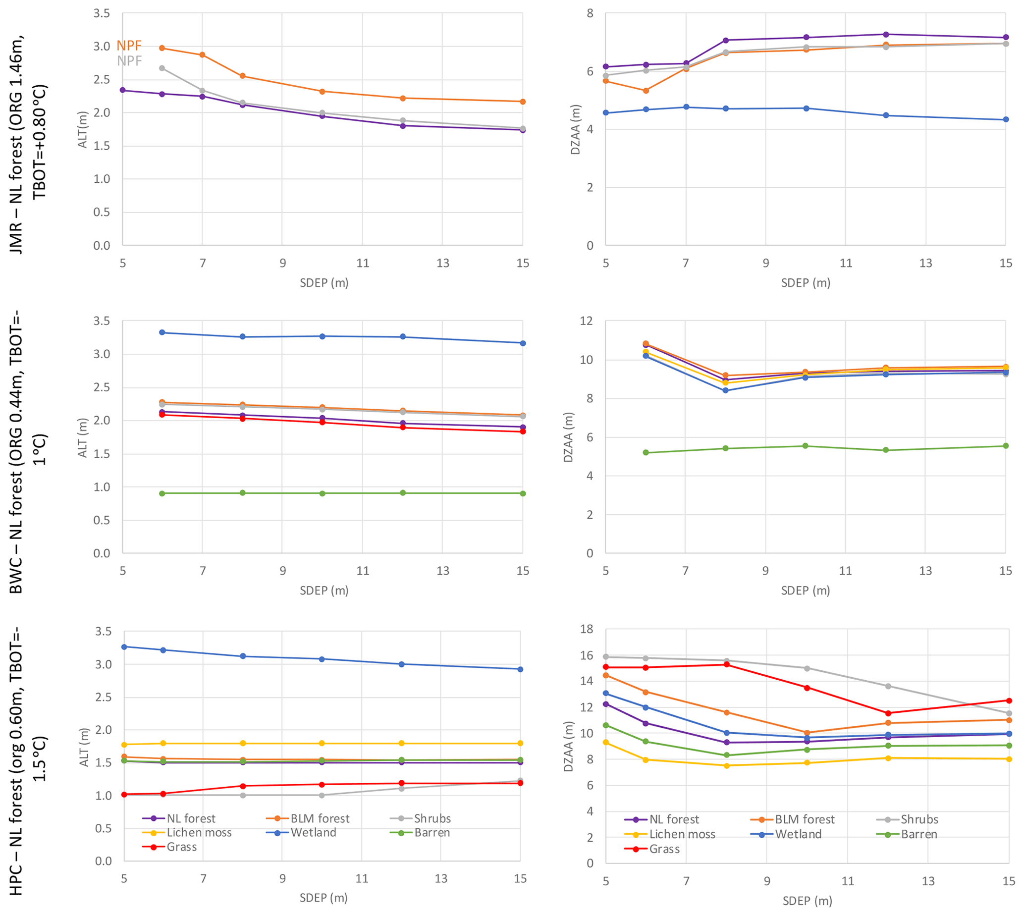
Figure 12Impact of SDEP on the average simulated ALT and DZAA for different GRUs at the three study sites over the 1980–2016 period. NPF: no permafrost.
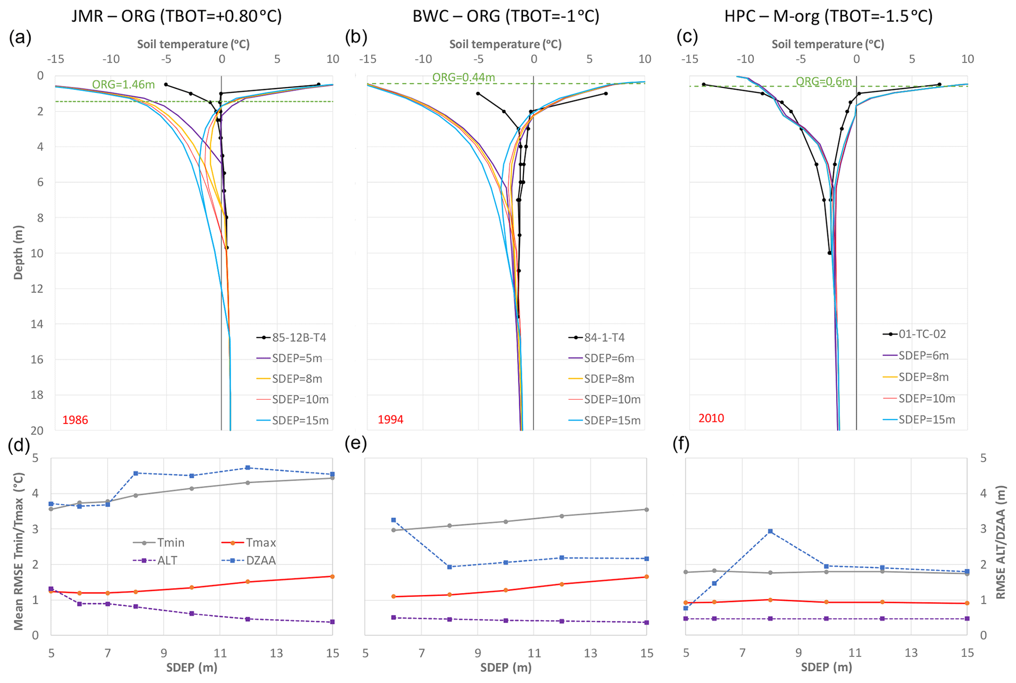
Figure 13Impact of SDEP on simulated temperature envelopes for a selected year at each study site (a–c). RMSE for temperature envelopes (Tmax and Tmin), ALT and DZAA (d–f) over the simulation period for the needleleaf forest GRU at each study site.
Figure 13 (top) shows how these changes to ALT and DZAA are occurring via changes in the shape of the temperature envelopes for a selected year. Increasing SDEP actually allows for more cooling of the middle soil layers (between 0.5–10 m), which pushes the maximum envelope upwards reducing ALT. The envelopes bend again to reach the specified bottom temperature, which is much clearer for JMR (because it is set to +0.80 ∘C) than BWC and HPC where it is set to a negative value. Differences across the SDEP range are small for HPC because of the M-org configuration. The straighter envelopes of HPC tend to meet (i.e. at DZAA) at larger depths than the curved ones at BWC and JMR. This cooling effect is possibly related to having moisture, especially ice, in deeper soil layers with a deeper SDEP, which affects the thermal properties of the soil. The presence of ice increases the thermal conductivity of the soil in general, compared to dry soil (see Sect. S1 in the Supplement). The bottom panel of Fig. 13 summarizes the impact of SDEP on RMSE for ALT, DZAA, Tmax, and Tmin over the simulation periods (years with observations as shown in Fig. 11). There are trade-offs in simulating the various aspects, as the minimum RMSE values are obtained at the maximum SDEP used for Tmin, Tmax, and DZAA at JMR and BWC, while the minimum RMSE values for ALT are obtained at the maximum used SDEP value. Except for ALT, RMSE seems insensitive to SDEP at HPC.
3.4 Impact of bottom temperature (TBOT)
As shown by the spin-up experiments above, the initial temperature of the deepest layer remains virtually unchanged through the spin-up and thus has to be specified. It was expected that simulations might converge to a possibly different steady state value at the end of spin-up, but they did not. The bottom of soil column has a constant flux boundary condition (Sect. 2.1). We used the default zero value for this constant, implying no gradient at the bottom, while TBOT is only an initial condition for the first spin-up cycle. We also tested values for the geothermal flux of 0.083 W m−2 at the three sites and found a negligible impact confirming the previous findings of Sapriza-Azuri et al. (2018). This value for the heat flux is the maximum of the range specified for western Canada by Garland and Lennox (1962). Temperature observations as deep as 50 m are rare, and relationships between that temperature and air or near-surface soil temperature are neither available nor appropriate. For the studied sites, it has been estimated from the observed profiles, and perturbed within a range of −3.0 to +1.5 ∘C, which was varied depending on the site condition and location. Figure 14 shows the impact of changing the temperature of the deepest layer on ALT and DZAA. For JMR, increasing TBOT increases ALT quickly so that taliks form under wetlands if TBOT >0 ∘C, and other land cover types follow at higher temperatures such that permafrost does not develop under most canopy types if TBOT >1.5 ∘C. This gives a way to simulate the no permafrost conditions observed at all sites in the basin (except 85-12B-T4). A similar relationship is simulated for BWC, as increasing TBOT increases ALT especially for wetlands. ALT at HPC is insensitive to TBOT because of the generally colder conditions and thicker permafrost. DZAA is showing low sensitivity to TBOT except for wetlands at JMR.
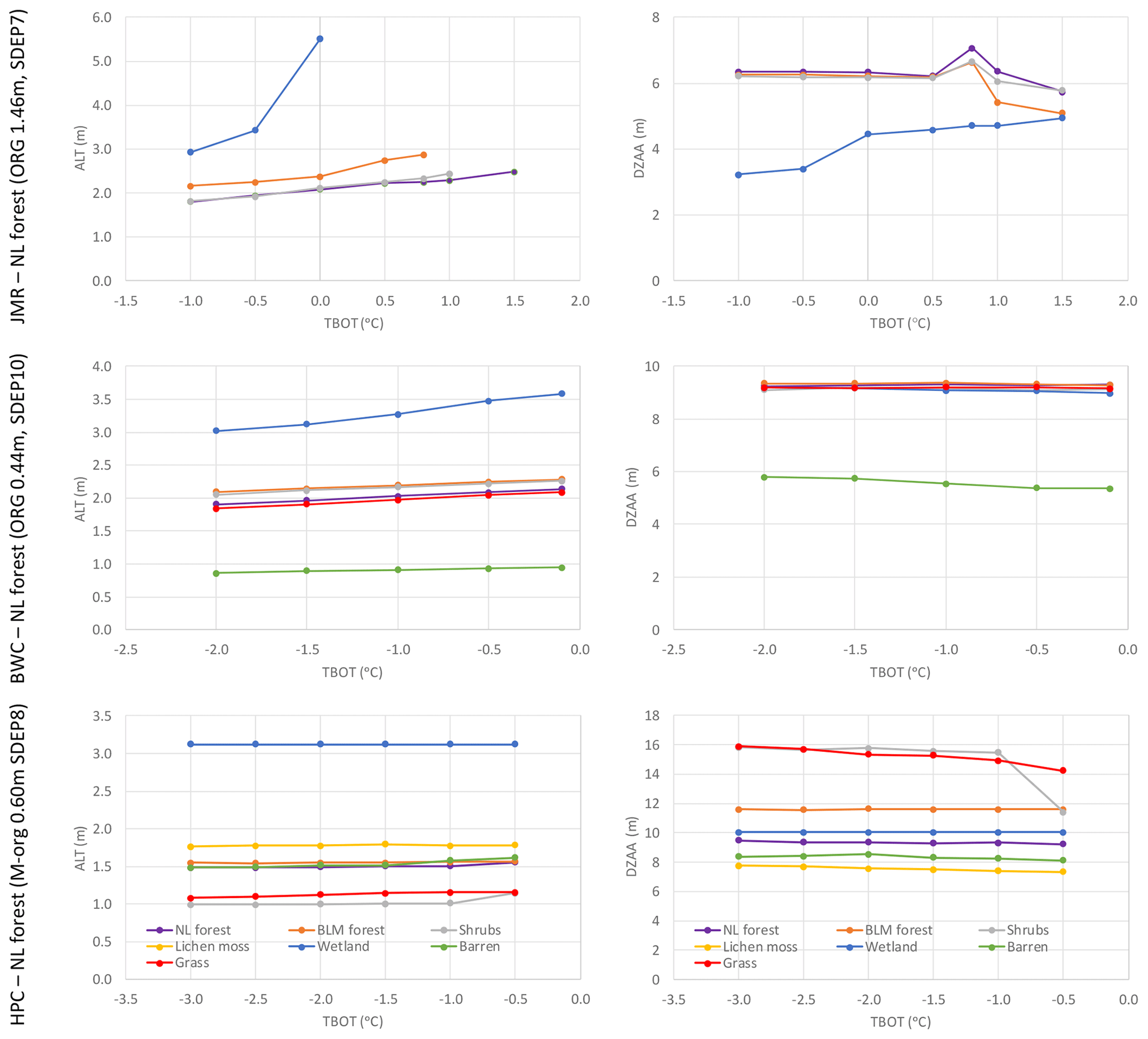
Figure 14Impact of TBOT on the average simulated ALT and DZAA for different GRUs at the three study sites over the 1980–2016 period.
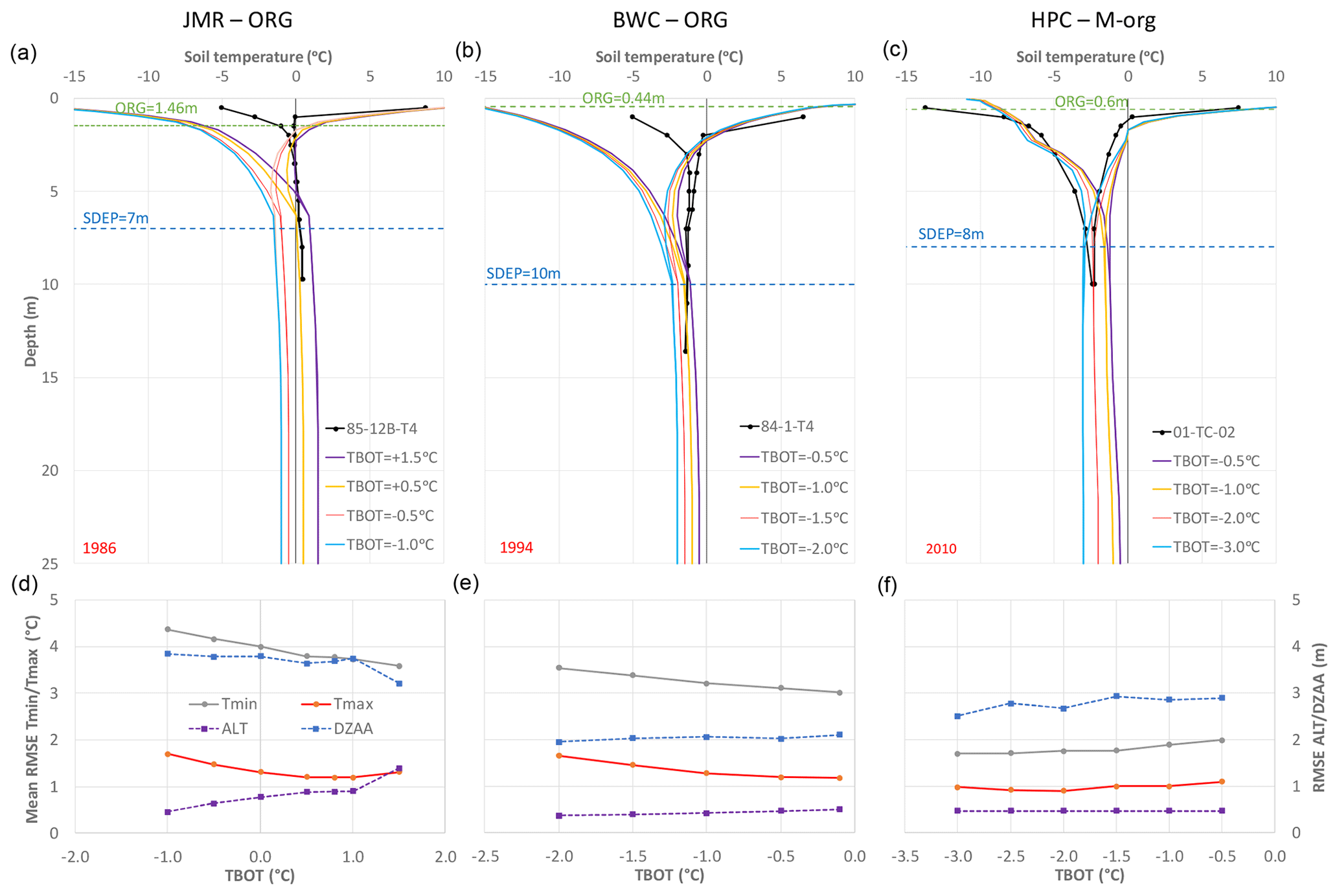
Figure 15Impact of TBOT on simulated temperature envelopes for a selected year at each study site (a–c). RMSE for temperature envelopes (Tmax and Tmin), ALT and DZAA (d–f) over the simulation period for the needleleaf forest GRU at each study site.
Figure 15 (top) shows how the temperature envelopes respond to changes in TBOT. In all cases, the envelopes seem to bend at some depth to try to reach the given bottom temperature. SDEP seems to influence the start of that inflection. This bending towards the given temperature causes another inflection of the maximum envelope closer to the surface. Depending on the depth of that first inflection, ALT may or may not be affected. DZAA is not affected as much, but the temperature at DZAA depends on TBOT. There is a noticeable difference between the M-org configuration of HPC on one hand and the ORG configuration at JMR and BWC on the other. Figure 15 (bottom) shows the impact of TBOT on model performance as measured by RMSE of ALT, DZAA, Tmin, and Tmax. Again we see trade-offs between getting the proper shape for the envelopes (as measured by RMSE for Tmax and Tmin) and ALT for JMR, indicating that a range between 0.5 to 1.0 ∘C for TBOT produces reasonable performance across the four metrics. For BWC, ALT and DZAA have a low sensitivity to TBOT at a range of −0.5 to −1 ∘C, which produces the best overall performance. For HPC, the colder the TBOT, the lower the RMSE values are for most metrics, with a value around −2 ∘C being reasonable.
3.5 Impact of organic depth (ORG) and configuration
It is believed that organic soils provide insulation to the impacts of the atmosphere on the soil temperature, which would lead to a thinner active layer than in a fully mineral soil. This assumption has been tested for the three sites by changing the depth of the fully organic layers for JMR and BWC as well as the mineral layers containing organic content at HPC. The results are sometimes counterintuitive. Peat plateaux are widespread in the JMR region, and thus the fully organic layers are followed by layers of high organic content (50 %) until SDEP. Increasing the fully organic layers initially reduces ALT (Fig. 16) as expected, but it also reduces DZAA quickly. Then ALT (which is defined mainly by the maximum temperature envelope) increases again which means that a deeper fully organic layer provides less insulation. The reason is related to the thermal and hydraulic properties of the peat. BWC exhibits different behaviour to JMR as ALT increases initially, when increasing the fully organic layers from three to four then decreases gradually. DZAA seems to decrease with an increasing organic depth for most land cover types at the three sites. DZAA and ALT show little sensitivity to the depth organic layers at HPC because the thermal and hydraulic properties under the M-org configuration are affected by the sand and clay fractions, while they are set to specific values for fully organic soils. Wetlands behave in a different way compared to other land cover types at the different sites because they are configured to remain close to saturation as much as possible. At JMR, wetlands are not underlain by permafrost for all organic configurations, which agrees with the literature.
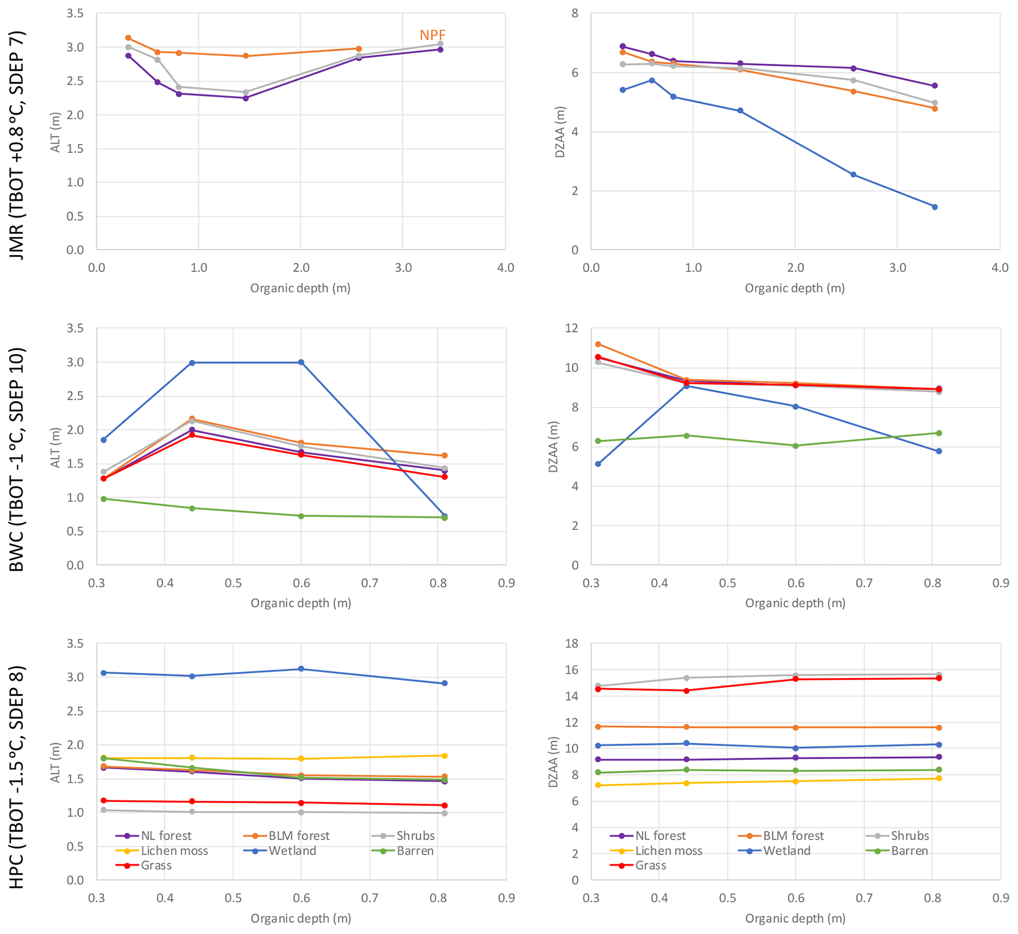
Figure 16Impact of the depth of organic soil layers on the average simulated ALT and DZAA for different GRUs at the three study sites for the 1980–2016 period. NPF: no permafrost.
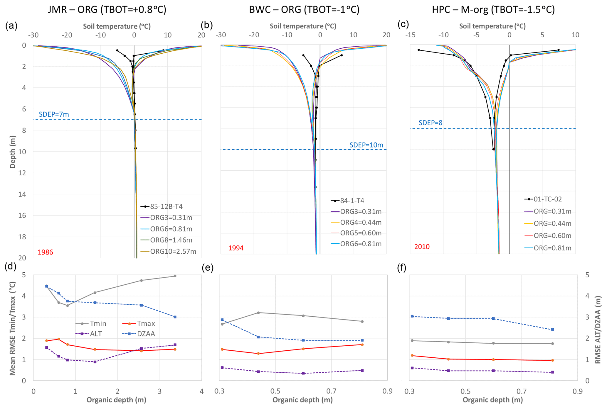
Figure 17Impact of organic depth on simulated temperature envelopes for a selected year at each study site (a–c). RMSE for temperature envelopes (Tmax and Tmin), ALT and DZAA (d–f) over the simulation period for the needleleaf forest GRU at each study site.
Figure 17 (top) shows the response of the temperature envelopes to changes in the organic depth. Increasing the organic depth causes much larger negative temperatures near the surface for the minimum envelope for ORG, but it causes the inflection of the minimum envelope to occur at slightly higher temperatures. A similar, but smaller, effect can be seen for the maximum envelope. The maximum envelopes for the different organic depth intersect, which corroborates with the above results for ALT. Another interesting feature can be observed comparing the ORG and M-org configurations. The M-org configurations has a much smaller temperature range near the surface than the fully organic soil and causes less cooling in the intermediate soil layers (above SDEP) such that the observed profiles are better matched to HPC. The high thermal capacity of the peat combined with its high thermal conductivity when containing ice in winter causes this cooling at the surface (Dobinski, 2011).
Figure 17 (bottom) summarizes the impact of organic depth (ORG for JMR and BWC; M-org for HPC) on the RMSE of ALT, DZAA, and the temperature envelopes. The impact in JMR is interesting as there are clear optimal values for ALT and Tmin and, to some extent, Tmax, although the optimal value is not the same for each aspect, leading to trade-offs. The selected 1.46 m depth (eight ORG layers) provides the best performance overall. For BWC, RMSE for Tmax and Tmin move in opposite directions (Tmin RMSE generally reduces, while Tmax RMSE increases with a deeper ORG). A depth around 0.5 m is generally satisfactory. For HPC, depths containing organic matter less then 0.6 m provide the optimal performance across the different aspects. A multi-criteria calibration framework can be set up using those performance metrics if the aim is the find the best configuration (including SDEP and TBOT) for each site. However, we are seeking generic rules that can be applied at larger scales, such as that of the MRB as a whole.
Permafrost is an important feature of cold regions, such as the Mackenzie River basin, and needs to be properly represented in land surface hydrological models, especially under the unprecedented climate warming trends that have been observed in these regions. The current generation of LSMs is being improved to simulate permafrost dynamics by allowing deeper soil profiles than typically used and incorporating organic soils explicitly. Deeper soil profiles have larger hydraulic and thermal memories that require more effort to initialize. We followed the recommendations of previous studies (e.g. Lawrence et al., 2012; Sapriza-Azuri et al., 2018) to select the total soil column depth to be around 50 m. The temperature envelopes meet (at DZAA) well within the 50 m soil column over the simulation period (including spin-up), such that the bottom boundary condition is not disturbing the simulated temperature profiles and envelopes and ALT.
We analysed the conventional layering schemes used by other LSMs, which tend to use an exponential formulation to maximize the number of layers near the surface and minimize the total number of layers (Oleson et al., 2013; Park et al., 2014). We found that the exponential formulation is not adequate to capture the dynamics of the active-layer depth and thus tested two other alternative schemes that have smaller thicknesses for the first 2 m, instead of the conventional ones. The first scheme had equally sized layers in the first metre, followed by thicker but equally sized layers in the second metre. The second scheme was formulated to have increasing thicknesses with depth following a scaled power law, which we found to be more suitable for the explicit forward numerical solution used by CLASS.
We discussed the common initialization approaches, including spinning up the model repeatedly using a single year (e.g. Dankers et al., 2011; Nishimura et al., 2009) or a sequence of years (e.g. Park et al., 2013), spinning up the model in a transient condition on long paleo-climatic records (e.g. Ednie et al., 2008), or combining both of these approaches (Sapriza-Azuri et al., 2018). Paleo-climatic reconstructions are scarce and provide limited information (e.g. mean summer temperature or total annual precipitation), while LSMs typically require a suite of meteorological variables at a high temporal resolution for the whole study domain. These variables can be stochastically generated at the resolution of interest informed by paleo-records. However, such practice is computationally expensive, especially for large domains and also introduces additional uncertainties. The approach of spinning up using available 20th-century data has been criticized as picking up the anthropogenic climate warming signal that started around 1850, thus yielding initial conditions that are not representative. However, paleo-climatic records also show that the climate has always been transient, and there may not exist a period of quasi-equilibrium long enough to start the spin-up process (Razavi et al., 2015). Spinning up using a sequence of years is thus more prone to having a trend than a single year, and detrending the sequence is not free of assumptions either.
Given the above complications, we investigated the impact of the simplest approach, which is spinning up using a single year (similar to Burke et al., 2013; Dankers et al., 2011), on several permafrost metrics (active-layer depth, depth of zero annual amplitude, and annual temperature envelopes). The aim was to determine the minimum number of spin-up cycles to have satisfactory performance (if reached) and to know how much accuracy is lost by not spinning more. We did this for three sites along a south–north transect in the Mackenzie River valley sampling the different permafrost zones (sporadic, extensive discontinuous, and continuous) in order to be able to generalize the findings to the whole MRB domain. Additionally, we investigated the sensitivity of the results to some important parameters such as the depth to bedrock, the temperature of the deepest layer, and the configuration of organic soil.
The results show that temperature profiles at the end of the spinning cycles remained virtually unchanged (i.e. reached a quasi steady state) after 50–100 cycles, when benchmarked against the results of 2000 cycles. We focused on temperature profiles for this stability analysis because we found that the soil moisture profiles (both liquid and frozen) stabilize much earlier during spin-up. In some cases, changes in the middle layers occurred after 100 cycles, but the influence of that on the simulated envelopes, ALT, and DZAA was found to be small to negligible compared to the uncertainty of observations and the scale of our model. We also found that the selection of the layering scheme has an effect on stabilization, and our proposed scheme with increasing thicknesses at depth reached stability faster and had less drifting. Therefore, the simple single-year spinning approach seems to be sufficient for our purpose using SC2. This agrees with Dankers et al. (2011), who showed that a higher vertical resolution improved the simulation of ALT using JULES.
We also found that the temperature of the deepest soil layer remained virtually unchanged from the specified initial value even after 2000 spinning cycles. Therefore, this temperature has to be specified by the modeller. For the study sites, we extrapolated it from the observed envelopes and studied the effect of perturbing it around the extrapolated value. This perturbation had small impacts on ALT and DZAA, except for JMR, which is located in the sporadic permafrost zone, but it had a significant impact on the shape of the envelopes. Temperature observations going as deep as 50 m are rare. Most of the permafrost monitoring sites in the MRB have up to 20 m cables, and thus we do not know whether the temperature of deeper soil layers has been changing over time, and if so, by how much. Changes in temperature at the deepest sensors at each of the three sites can be seen in Fig. S1 of the Supplement. To take the information back to the large scale, we recommend using a south–north gradient moving from +1.0 in the sporadic zone to -2.0 in the continuous zone and specifying a spatially variable field as an input initial condition. These effects show the regional variability which needs to be assessed for different applications such as other basins affected by permafrost or by using other LSMs. This could lead to the verification of such a finding and to the preparation of a global map of initial values for TBOT by combining observations and modelling. We have not seen such detailed analyses in the literature.
For this study, we tested whether a non-zero thermal flux boundary condition could resolve this issue, but the impacts were negligible using the literature values for the geothermal flux (0.083 W m−2) in the region. However, available datasets for the geothermal flux (e.g. Bachu, 1993) are not transient and estimate those fluxes at depths greater than the 50 m used. Our results agree with those of Nishimura et al. (2009) and Sapriza-Azuri et al. (2018), who showed that the geothermal heat flux had a negligible effect on most simulations in study areas in Siberia and Canada, respectively. Nevertheless, the issue may need further investigation using other models (including thermal ones) and tests in other regions before generalizing such conclusions.
The analyses also demonstrated the importance of the organic soil configuration (i.e. number of layers and their parameterization respective of organic sub-types) on the simulated temperature profiles and active-layer dynamics. This has been illustrated in the literature. For example, Dankers et al. (2011) found that adjusting soil parameters for organic content has relatively little effect on ALT simulations of the Arctic region, while Nicolsky et al. (2007) and Park et al. (2013) stressed the importance of organic content to the fidelity of permafrost simulations. Park et al. (2013) further indicated that organic matter evolves dynamically as it decomposes over time and depends on biogeochemical processes such as plant growth, root development, and littering. This could be simulated in LSMs by including the carbon cycle. However, fully organic soils were not extensively tested in a permafrost context as shown in our study.
In most cases, we found combinations of TBOT, SDEP, and ORG that produced satisfactory simulations, but the impact of organic layering seems to require further investigation, as increasing the thickness of organic layers does not always act to reduce ALT or reduce the cooling in the middle soil layers that should result from increased insulation. There is an interplay between the moisture properties and content and thermal properties of organic soils that needs further investigation. Additionally, we cannot represent stacked canopies using CLASS, e.g. trees or shrubs underlain by moss or the effect of litter under (deciduous) trees and shrubs. Moss or litter could be providing additional insulation under those canopies that is not represented. The quality of snow simulations can also impact the quality of permafrost simulations. For example, Burke et al. (2013) showed that a multi-layer snow model improved ALT simulations in JULES; CLASS has a single-layer snow model.
To conclude, we have formulated a generic approach to represent permafrost within the MESH framework (running CLASS) for applications at large scales that has the following features:
-
a 50 m deep soil profile with increasing soil thickness with depth;
-
50–100 spinning cycles of the first year of record to initialize the moisture and temperature profiles; and
-
spatially distributed TBOT, SDEP, and soil texture parameters, with a systematic guideline to use the 30 % threshold to identify fully organic soils.
The generic nature of this approach comes from testing it at three sites within different permafrost classes (sporadic, discontinuous, and continuous). However, testing the approach is other regions, and with other LSMs (e.g. CLM and MESH/SVS), is necessary before pursuing it for wider applications. This can be done using representative sub-basins where permafrost observations exist to test the above-mentioned elements and make any necessary adjustments for application at large scales. Additionally, this study demonstrated a simple and effective way to use small-scale investigations to inform larger-scale modelling. While the GRU-based parameterization approach facilitates such transferability, the key is to use the same physics at both scales.
It was necessary to increase the flexibility of the MESH framework to accommodate these input formats as well as to produce relevant permafrost outputs. However, the model is still deficient in some ways. For example, the explicit forward numerical solution may limit how soil layering should be defined. The lack of complex canopies, the use of a single-layer snow model, and the static nature of soil organic content may be affecting our parameterization of MESH. The parameterization of bedrock as sandstone requires further investigation, as it does not reflect the spatial variability of thermal properties of bedrock material. These findings are not specific to MESH or CLASS and could be beneficial for the LSM community in general. Therefore, further analysis and model development is required towards improving the realism of the simulations in permafrost regions. It is vitally required to incorporate key features of permafrost dynamics (e.g. taliks, land subsidence, and thermokarst) into LSMs, as well as the linkages between permafrost evolution phase (aggradation and degradation) and carbon–climate feedback cycles under the changing climatic conditions. The inclusion of such features could enhance the representation of hydrological processes within LSMs and, consequently, ESMs. Accordingly, there is a pressing need to promote multidisciplinary research in permafrost territories among hydrologists, climatologists, geomorphologists, and geotechnical engineers.
MESH code is available from the MESH wiki page (https://wiki.usask.ca/display/MESH/Releases; University of Saskatchewan, 2019).
Distributed soil texture and SDEP data are available from Keshav et al. (2019b, a). Permafrost observations were collected from various reports of Geological Survey Canada as referenced in the paper.
The supplement related to this article is available online at: https://doi.org/10.5194/hess-24-349-2020-supplement.
MEE, AP and HSW conceived the experimental design of this study. GSA provided the original MESH setup of the MRB. GSA and MEE collected the permafrost observations. DP provided the MESH code and implemented the necessary code changes. MEE conducted the simulation work and analyzed the results. MSA participated in the interpretation of results and preparation of some illustrations. MEE prepared the paper with contributions from all co-authors.
The authors declare that they have no conflict of interest.
This article is part of the special issue “Understanding and predicting Earth system and hydrological change in cold regions”. It is not associated with a conference.
This research was undertaken as part of the Changing Cold Regions Network. The Canada Excellence Research Chair (CERC) in Water Security at the University of Saskatchewan supported a number of co-authors and provided the facilities. We gratefully acknowledge the contribution of two anonymous reviewers to the improvement of the paper.
This research has been supported by the Natural Sciences and Engineering Research Council of Canada (grant for the Changing Cold Regions Network).
This paper was edited by Sean Carey and reviewed by two anonymous referees.
Alexeev, V. A., Nicolsky, D. J., Romanovsky, V. E., and Lawrence, D. M.: An evaluation of deep soil configurations in the CLM3 for improved representation of permafrost, Geophys. Res. Lett., 34, L09502, https://doi.org/10.1029/2007GL029536, 2007.
Arboleda-Obando, P.: Determinando los efectos del cambio climático y del cambio en usos del suelo en la Macro Cuenca Magdalena Cauca utilizando el modelo de suelo-superficie e hidrológico MESH, available at: http://bdigital.unal.edu.co/69823/1/1018438123.2018.pdf (last access: 18 April 2019), 2018.
Bachu, S.: Basement heat flow in the Western Canada Sedimentary Basin, Tectonophysics, 222, 119–133, https://doi.org/10.1016/0040-1951(93)90194-O, 1993.
Bahremand, A., Razavi, S., Pietroniro, A., Haghnegahdar, A., Princz, D., Gharari, S., Elshamy, M., and Tesemma, Z.: Application of MESH Land Surface-Hydrology Model to a Large River Basin in Iran Model Prospective works, in: Canadian Geophysical Union General Assembly, 10–14 June 2018, Niagara Falls, Canada, p. 3, 2018.
Best, M. J., Pryor, M., Clark, D. B., Rooney, G. G., Essery, R. L. H., Ménard, C. B., Edwards, J. M., Hendry, M. A., Porson, A., Gedney, N., Mercado, L. M., Sitch, S., Blyth, E., Boucher, O., Cox, P. M., Grimmond, C. S. B., and Harding, R. J.: The Joint UK Land Environment Simulator (JULES), model description – Part 1: Energy and water fluxes, Geosci. Model Dev., 4, 677–699, https://doi.org/10.5194/gmd-4-677-2011, 2011.
Bonsal, B. R., Peters, D. L., Seglenieks, F., Rivera, A., and Berg, A.: Changes in freshwater availability across Canada, in: Canada's Changing Climate Report, 261–342, available at: https://www.nrcan.gc.ca/sites/www.nrcan.gc.ca/files/energy/Climate-change/pdf/CCCR-Chapter6-ChangesInFreshwaterAvailabilityAcrossCanada.pdf, last access: 27 August 2019.
Burke, E. J., Dankers, R., Jones, C. D., and Wiltshire, A. J.: A retrospective analysis of pan Arctic permafrost using the JULES land surface model, Clim. Dynam., 41, 1025–1038, https://doi.org/10.1007/s00382-012-1648-x, 2013.
Burn, C. R. and Nelson, F. E.: Comment on “A projection of severe near-surface permafrost degradation during the 21st century” by David M. Lawrence and Andrew G. Slater, Geophys. Res. Lett., 33, L21503, https://doi.org/10.1029/2006gl027077, 2006.
Calmels, F., Laurent, C., Brown, R., Pivot, F., and Ireland, M.: How Permafrost Thaw May Impact Food Security of Jean Marie River First Nation, NWT, GeoQuebec 2015 Conf. Pap., 20–23 September 2015, Quebec City, Canada, 2015.
Canada Centre for Remote Sensing (CCRS), Nacional para el Conocimiento y Uso de la Biodiversidad (CONABIO), Comisión Nacional Forestal (CONAFOR), Insituto Nacional de Estadística y Geografía (INEGI), and U.S. Geological Survey (USGS): 2005 North American Land Cover at 250 m spatial resolution, available at: http://www.cec.org/tools-and-resources/map-files/land-cover-2005 (last access: 15 January 2016), 2010.
Centre for Land and Biological Resources Research: Soil Landscapes of Canada, v.2.2, Research Branch, Agriculture and Agri-Food Canada, Ottawa, Canada, 1996.
Changwei, X. and Gough, W. A.: A Simple Thaw-Freeze Algorithm for a Multi-Layered Soil using the Stefan Equation, Permafrost Periglac., 24, 252–260, https://doi.org/10.1002/ppp.1770, 2013.
Côté, J., Gravel, S., Méthot, A., Patoine, A., Roch, M., Staniforth, A., Côté, J., Gravel, S., Méthot, A., Patoine, A., Roch, M., and Staniforth, A.: The Operational CMC–MRB Global Environmental Multiscale (GEM) Model. Part I: Design Considerations and Formulation, Mon. Weather Rev., 126, 1373–1395, https://doi.org/10.1175/1520-0493(1998)126<1373:TOCMGE>2.0.CO;2, 1998a.
Côté, J., Desmarais, J.-G., Gravel, S., Méthot, A., Patoine, A., Staniforth, A., and Roch, M.: The Operational CMC – MRB Global Environmental Multiscale (GEM) Model. Part II: Results, Mon. Weather Rev., 126, 1397–1418, https://doi.org/10.1175/1520-0493(1998)126<1397:TOCMGE>2.0.CO;2, 1998b.
Dankers, R., Burke, E. J., and Price, J.: Simulation of permafrost and seasonal thaw depth in the JULES land surface scheme, The Cryosphere, 5, 773–790, https://doi.org/10.5194/tc-5-773-2011, 2011.
DeBeer, C. M., Wheater, H. S., Carey, S. K., and Chun, K. P.: Recent climatic, cryospheric, and hydrological changes over the interior of western Canada: a review and synthesis, Hydrol. Earth Syst. Sci., 20, 1573–1598, https://doi.org/10.5194/hess-20-1573-2016, 2016.
Dobinski, W.: Permafrost, Earth-Sci. Rev., 108, 158–169, https://doi.org/10.1016/J.EARSCIREV.2011.06.007, 2011.
Duan, L., Man, X., Kurylyk, B. L., and Cai, T.: Increasing winter baseflow in response to permafrost thaw and precipitation regime shifts in northeastern China, Water, 9, 25, https://doi.org/10.3390/w9010025, 2017.
Durocher, M., Requena, A. I., Burn, D. H., and Pellerin, J.: Analysis of trends in annual streamflow to the Arctic Ocean, Hydrol. Process., 33, 1143–1151, https://doi.org/10.1002/hyp.13392, 2019.
Ednie, M., Wright, J. F., and Duchesne, C.: Establishing initial conditions for transient ground thermal modeling in the Mackenzie Valley: a paleo-climatic reconstruction approach, in: Proceedings of the Ninth International Conference on Permafrost, edited by: Kane, D. L. and Hinkel, K. M., 29 June–3 July 2008, Institute of Northern Engineering, University of Alaska Fairbanks, Fairbanks, Alaska, USA, 403–408, 2008.
Elshamy, M. E., Pietroniro, A., and Wheater, H. S.: Development and validation of a large-scale hydrological land surface model for the Mackenzie River Basin, in preparation, 2020.
Garland, G. D. and Lennox, D. H.: Heat Flow in Western Canada, Geophys. J. Roy. Astr. S., 6, 245–262, https://doi.org/10.1111/j.1365-246X.1962.tb02979.x, 1962.
Haghnegahdar, A., Tolson, B. A., Craig, J. R., and Paya, K. T.: Assessing the performance of a semi-distributed hydrological model under various watershed discretization schemes, Hydrol. Process., 29, 4018–4031, https://doi.org/10.1002/hyp.10550, 2015.
Hegginbottom, J. A., Dubreuil, M. A., and Harker, P. T.: Permafrost, in: National Atlas of Canada, MCR 4177, Natural Resources Canada, https://doi.org/10.4095/294765, 1995.
Husain, S. Z., Alavi, N., Bélair, S., Carrera, M., Zhang, S., Fortin, V., Abrahamowicz, M., Gauthier, N., Husain, S. Z., Alavi, N., Bélair, S., Carrera, M., Zhang, S., Fortin, V., Abrahamowicz, M., and Gauthier, N.: The Multibudget Soil, Vegetation, and Snow (SVS) Scheme for Land Surface Parameterization: Offline Warm Season Evaluation, J. Hydrometeorol., 17, 2293–2313, https://doi.org/10.1175/JHM-D-15-0228.1, 2016.
IPCC: Climate Change 2014 Impacts, Adaptation, and Vulnerability Part B: Regional Aspects, edited by: Barros, V. R., Field, C. B., Dokken, D. J., Mastrandrea, M. D., Mach, K. J., Bilir, T. E., Chatterjee, M., Ebi, K. L., Estrada, Y. O., Genova, R. C., Girma, B., Kissel, E. S., Levy, A. N., MacCracken, S., Mastrandrea, P. R., and White, L. L., Cambridge University Press, Cambridge, UK and New York, NY, USA, 2014.
Keshav, K., Haghnegahdar, A., Elshamy, M., Gharari, S., and Razavi, S.: Aggregated gridded soil texture dataset for Mackenzie and Nelson-Churchill River Basins, Federated Research Data Repository (FRDR), Canada, https://doi.org/10.20383/101.0154, 2019a.
Keshav, K., Haghnegahdar, A., Elshamy, M., Gharari, S., and Razavi, S.: Bedrock depth dataset for Nelson-Churchill and Mackenzie River Basin based on bedrock data by Shangguan et al. (2016), Federated Research Data Repository (FRDR), Canada, https://doi.org/10.20383/101.0152, 2019b.
Kouwen, N.: WATFLOOD: a Micro-Computer Based Flood Forecasting System Based on Real-Time Weather Radar, Can. Water Resour. J., 13, 62–77, https://doi.org/10.4296/cwrj1301062, 1988.
Kouwen, N., Soulis, E. D., Pietroniro, A., Donald, J., and Harrington, R. A.: Grouped Response Units for Distributed Hydrologic Modeling, J. Water Resour. Plan. Manag., 119, 289–305, https://doi.org/10.1061/(ASCE)0733-9496(1993)119:3(289), 1993.
Krogh, S. A., Pomeroy, J. W., and Marsh, P.: Diagnosis of the hydrology of a small Arctic basin at the tundra-taiga transition using a physically based hydrological model, J. Hydrol., 550, 685–703, https://doi.org/10.1016/j.jhydrol.2017.05.042, 2017.
Kujala, K., Seppälä, M., and Holappa, T.: Physical properties of peat and palsa formation, Cold Reg. Sci. Technol., 52, 408–414, https://doi.org/10.1016/j.coldregions.2007.08.002, 2008.
Lawrence, D. M. and Slater, A. G.: A projection of severe near-surface permafrost degradation during the 21st century, Geophys. Res. Lett., 32, L24401, https://doi.org/10.1029/2005GL025080, 2005.
Lawrence, D. M., Slater, A. G., Romanovsky, V. E., and Nicolsky, D. J.: Sensitivity of a model projection of near-surface permafrost degradation to soil column depth and representation of soil organic matter, J. Geophys. Res.-Earth, 113, 1–14, https://doi.org/10.1029/2007JF000883, 2008.
Lawrence, D. M., Slater, A. G., and Swenson, S. C.: Simulation of present-day and future permafrost and seasonally frozen ground conditions in CCSM4, J. Climate, 25, 2207–2225, https://doi.org/10.1175/JCLI-D-11-00334.1, 2012.
Letts, M. G., Roulet, N. T., Comer, N. T., Skarupa, M. R., and Verseghy, D. L.: Parameterization of Peatland Hydraulic Properties for the Canadian Land Surface Scheme, Atmos.-Ocean, 38, 141–160, https://doi.org/10.1080/07055900.2000.9649643, 2000.
Luo, Y., Arnold, J., Allen, P., and Chen, X.: Baseflow simulation using SWAT model in an inland river basin in Tianshan Mountains, Northwest China, Hydrol. Earth Syst. Sci., 16, 1259–1267, https://doi.org/10.5194/hess-16-1259-2012, 2012.
Mahfouf, J.-F., Brasnett, B., and Gagnon, S.: A Canadian Precipitation Analysis (CaPA) Project: Description and Preliminary Results, Atmos.-Ocean, 45, 1–17, https://doi.org/10.3137/ao.v450101, 2007.
McBean, G., Alekseev, G., Chen, D., Førland, E., Fyfe, J., Groisman, P. Y., King, R., Melling, H., Vose, R., and H.Whitfield, P.: Arctic Climate: Past and Present, in: Impacts of a Warming Arctic: Arctic Climate Impact Assessment, Cambridge University Press, Canada, p. 140, 2005.
Nicolsky, D. J., Romanovsky, V. E., Alexeev, V. A., and Lawrence, D. M.: Improved modeling of permafrost dynamics in a GCM land-surface scheme, Geophys. Res. Lett., 34, 2–6, https://doi.org/10.1029/2007GL029525, 2007.
Nishimura, S., Martin, C. J., Jardine, R. J., and Fenton, C. H.: A new approach for assessing geothermal response to climate change in permafrost regions, Geotechnique, 59, 213–227, https://doi.org/10.1680/geot.2009.59.3.213, 2009.
Oleson, K. W., Lawrence, D. M., Bonan, G. B., Drewniak, B., Huang, M., Charles, D., Levis, S., Li, F., Riley, W. J., Zachary, M., Swenson, S. C., Thornton, P. E., Bozbiyik, A., Fisher, R., Heald, C. L., Kluzek, E., Lamarque, F., Lawrence, P. J., Leung, L. R., Muszala, S., Ricciuto, D. M., and Sacks, W.: Technical Description of version 4.5 of the Community Land Model (CLM), National Center For Atmospheric Research, Boulder, Colorado, USA, 2013.
Park, H., Iijima, Y., Yabuki, H., Ohta, T., Walsh, J., Kodama, Y., and Ohata, T.: The application of a coupled hydrological and biogeochemical model (CHANGE) for modeling of energy, water, and CO2 exchanges over a larch forest in eastern Siberia, J. Geophys. Res., 116, D15102, https://doi.org/10.1029/2010JD015386, 2011.
Park, H., Walsh, J., Fedorov, A. N., Sherstiukov, A. B., Iijima, Y., and Ohata, T.: The influence of climate and hydrological variables on opposite anomaly in active-layer thickness between Eurasian and North American watersheds, The Cryosphere, 7, 631–645, https://doi.org/10.5194/tc-7-631-2013, 2013.
Park, H., Sherstiukov, A. B., Fedorov, A. N., Polyakov, I. V., and Walsh, J. E.: An observation-based assessment of the influences of air temperature and snow depth on soil temperature in Russia, Environ. Res. Lett., 9, 064026, https://doi.org/10.1088/1748-9326/9/6/064026, 2014.
Pietroniro, A., Fortin, V., Kouwen, N., Neal, C., Turcotte, R., Davison, B., Verseghy, D., Soulis, E. D., Caldwell, R., Evora, N., and Pellerin, P.: Development of the MESH modelling system for hydrological ensemble forecasting of the Laurentian Great Lakes at the regional scale, Hydrol. Earth Syst. Sci., 11, 1279–1294, https://doi.org/10.5194/hess-11-1279-2007, 2007.
Pomeroy, J. W., Gray, D. M., Brown, T., Hedstrom, N. R., Quinton, W. L., Granger, R. J., and Carey, S. K.: The cold regions hydrological model: a platform for basing process representation and model structure on physical evidence, Hydrol. Process., 21, 2650–2667, https://doi.org/10.1002/hyp.6787, 2007.
Quinton, W. L. and Marsh, P.: A conceptual framework for runoff generation in a permafrost environment, Hydrol. Process., 13, 2563–2581, https://doi.org/10.1002/(SICI)1099-1085(199911)13:16<2563::AID-HYP942>3.0.CO;2-D, 1999.
Quinton, W. L., Hayashi, M., and Chasmer, L. E.: Permafrost-thaw-induced land-cover change in the Canadian subarctic: implications for water resources, Hydrol. Process., 25, 152–158, https://doi.org/10.1002/hyp.7894, 2011.
Razavi, S., Elshorbagy, A., Wheater, H., and Sauchyn, D.: Toward understanding nonstationarity in climate and hydrology through tree ring proxy records, Water Resour. Res., 51, 1813–1830, https://doi.org/10.1002/2014WR015696, 2015.
Riseborough, D., Shiklomanov, N., Etzelmüller, B., Gruber, S., and Marchenko, S.: Recent advances in permafrost modelling, Permafrost Periglac., 19, 137–156, https://doi.org/10.1002/ppp.615, 2008.
Romanovsky, V. E. and Osterkamp, T. E.: Interannual variations of the thermal regime of the active layer and near-surface permafrost in northern Alaska, Permafrost Periglac., 6, 313–335, https://doi.org/10.1002/ppp.3430060404, 1995.
Sapriza-Azuri, G., Gamazo, P., Razavi, S., and Wheater, H. S.: On the appropriate definition of soil profile configuration and initial conditions for land surface–hydrology models in cold regions, Hydrol. Earth Syst. Sci., 22, 3295–3309, https://doi.org/10.5194/hess-22-3295-2018, 2018.
Shangguan, W., Hengl, T., Mendes de Jesus, J., Yuan, H., and Dai, Y.: Mapping the global depth to bedrock for land surface modeling, J. Adv. Model. Earth Syst., 9, 65–88, https://doi.org/10.1002/2016MS000686, 2017.
Sheffield, J., Goteti, G., and Wood, E. F.: Development of a 50-year high-resolution global dataset of meteorological forcings for land surface modeling, J. Climate, 19, 3088–3111, https://doi.org/10.1175/JCLI3790.1, 2006.
Smith, S. L. and Burgess, M.: Ground Temperature Database for Northern Canada, Geological Survey of Canada Open File Report 3954, October 2000, Ottawa, Canada, 2000.
Smith, S. L. and Burgess, M. M.: A digital database of permafrost thickness in Canada, Geological Survey of Canada Open File 4173, Ottawa, Canada, 2002.
Smith, S. L., Burgess, M. M., Riseborough, D., Coultish, T., and Chartrand, J.: Digital summary database of permafrost and thermal conditions - Norman Wells pipeline study sites, Geol. Surv. Canada, Open File 4635, 4635, 1–104, https://doi.org/10.4095/215482, 2004.
Smith, S. L., Ye, S., and Ednie, M.: Enhancement of permafrost monitoring network and collection of baseline environmental data between Fort Good Hope and Norman Wells, Northwest Territories, Geological Survey of Canada, Current Research 2007-B7, 1–10, Ottawa, Canada, 2007.
Smith, S. L., Riseborough, D. W., Nixon, F. M., Chartrand, J., Duchesne, C., and Ednie, M.: Data for Geological Survey of Canada Active Layer Monitoring Sites in the Mackenzie Valley, N.W.T., Geological Survey Of Canada Open File 6287, Ottawa, Canada, 2009.
Smith, S. L., Chartrand, J., Duchesne, C., and Ednie, M.: Report on 2015 field activities and collection of ground thermal and active layer data in the Mackenzie corridor, Northwest Territories, Geol. Surv. Canada Open File 8125, https://doi.org/10.4095/292864, 2016.
Soil Classification Working Group: The Canadian system of soil classification, 3rd edn., NRC Research Press, Ottawa, Canada, available at: http://sis.agr.gc.ca/cansis/publications/manuals/1998-cssc-ed3/cssc3_manual.pdf (last access: 17 April 2019), 1998.
Soulis, E. D. E., Snelgrove, K. K. R., Kouwen, N., Seglenieks, F., and Verseghy, D. L. D.: Towards closing the vertical water balance in Canadian atmospheric models: Coupling of the land surface scheme class with the distributed hydrological model watflood, Atmos.-Ocean, 38, 251–269, https://doi.org/10.1080/07055900.2000.9649648, 2000.
St. Jacques, J. M. and Sauchyn, D. J.: Increasing winter baseflow and mean annual streamflow from possible permafrost thawing in the Northwest Territories, Canada, Geophys. Res. Lett., 36, L01401, https://doi.org/10.1029/2008GL035822, 2009.
Swenson, S. C., Lawrence, D. M., and Lee, H.: Improved simulation of the terrestrial hydrological cycle in permafrost regions by the Community Land Model, J. Adv. Model. Earth Syst., 4, 1–15, https://doi.org/10.1029/2012MS000165, 2012.
Szeicz, J. M. and MacDonald, G. M.: Dendroclimatic Reconstruction of Summer Temperatures in Northwestern Canada since A.D. 1638 Based on Age-Dependent Modeling, Quaternary Res., 44, 257–266, https://doi.org/10.1006/qres.1995.1070, 1995.
University of Saskatchewan: MESH – A Community Hydrology – Land Surface Model (Releases), available at: https://wiki.usask.ca/display/MESH/Releases, last access: 21 January 2019.
van Everdingen, R. O.: Multi-language Glossary of Permafrost and Related Ground-Ice Terms, International Permafrost Association, The Arctic Institute of North America, University of Calgary, Calgary, Canada, 2005.
Verseghy, D.: CLASS – The Canadian land surface scheme (version 3.6) - technical documentation, Intern. report, Clim. Res. Div. Sci. Technol. Branch, Environ. Canada, 2012.
Verseghy, D. L.: Class—A Canadian land surface scheme for GCMS. I. Soil model, Int. J. Climatol., 11, 111–133, https://doi.org/10.1002/joc.3370110202, 1991.
Walvoord, M. A. and Kurylyk, B. L.: Hydrologic Impacts of Thawing Permafrost – A Review, Vadose Zone J., 15, https://doi.org/10.2136/vzj2016.01.0010, 2016.
Walvoord, M. A. and Striegl, R. G.: Increased groundwater to stream discharge from permafrost thawing in the Yukon River basin: Potential impacts on lateral export of carbon and nitrogen, Geophys. Res. Lett., 34, L12402, https://doi.org/10.1029/2007GL030216, 2007.
Weedon, G. P., Gomes, S., Viterbo, P., Shuttleworth, W. J., Blyth, E., Österle, H., Adam, J. C., Bellouin, N., Boucher, O., and Best, M.: Creation of the WATCH Forcing Data and Its Use to Assess Global and Regional Reference Crop Evaporation over Land during the Twentieth Century, J. Hydrometeorol., 12, 823–848, https://doi.org/10.1175/2011JHM1369.1, 2011.
Weedon, G. P., Balsamo, G., Bellouin, N., Gomes, S., Best, M. J., and Viterbo, P.: The WFDEI meteorological forcing data set: WATCH Forcing Data methodology applied to ERA-Interim reanalysis data, Water Resour. Res., 50, 7505–7514, https://doi.org/10.1002/2014WR015638, 2014.
Wong, J. S., Razavi, S., Bonsal, B. R., Wheater, H. S., and Asong, Z. E.: Inter-comparison of daily precipitation products for large-scale hydro-climatic applications over Canada, Hydrol. Earth Syst. Sci., 21, 2163–2185, https://doi.org/10.5194/hess-21-2163-2017, 2017.
Wright, J. F., Duchesne, C., and Côté, M. M.: Regional-scale permafrost mapping using the TTOP ground temperature model, in: Proceedings of the Eighth International Conference on Permafrost, 21–25 July 2003, Zurich, Switzerland, 1241–1246, 2003.
Yassin, F., Razavi, S., Wheater, H., Sapriza-Azuri, G., Davison, B., and Pietroniro, A.: Enhanced identification of a hydrologic model using streamflow and satellite water storage data: A multicriteria sensitivity analysis and optimization approach, Hydrol. Process., 31, 3320–3333, https://doi.org/10.1002/hyp.11267, 2017.
Yassin, F., Razavi, S., Wong, J. S., Pietroniro, A., and Wheater, H.: Hydrologic-Land Surface Modelling of a Complex System under Precipitation Uncertainty: A Case Study of the Saskatchewan River Basin, Canada, Hydrol. Earth Syst. Sci. Discuss., https://doi.org/10.5194/hess-2019-207, 2019a.
Yassin, F., Razavi, S., Elshamy, M., Davison, B., Sapriza-Azuri, G., and Wheater, H.: Representation and improved parameterization of reservoir operation in hydrological and land-surface models, Hydrol. Earth Syst. Sci., 23, 3735–3764, https://doi.org/10.5194/hess-23-3735-2019, 2019b.
Yeh, K.-S., Côté, J., Gravel, S., Méthot, A., Patoine, A., Roch, M., Staniforth, A., Yeh, K.-S., Côté, J., Gravel, S., Méthot, A., Patoine, A., Roch, M., and Staniforth, A.: The CMC–MRB Global Environmental Multiscale (GEM) Model. Part III: Nonhydrostatic Formulation, Mon. Weather Rev., 130, 339–356, https://doi.org/10.1175/1520-0493(2002)130<0339:TCMGEM>2.0.CO;2, 2002.
Zhang, T., Barry, R. G., Knowles, K., Heginbottom, J. A., and Brown, J.: Polar Geography Statistics and characteristics of permafrost and ground-ice distribution in the Northern Hemisphere, Polar Geogr., 31, 47–68, https://doi.org/10.1080/10889370802175895, 2008.
Zhang, X., Flato, G., Kirchmeier-Young, M., Vincent, L., Wan, H., Wang, X., Rong, R., Fyfe, J., Li, G. and Kharin, V. V: Changes in Temperature and Precipitation Across Canada, in Canada's Changing Climate Report, 112–193, available at: https://changingclimate.ca/site/assets/uploads/sites/2/2018/12/CCCR-Chapter4-TemperatureAndPrecipitationAcrossCanada.pdf, last access: 22 April 2019.
Zhang, Y., Cheng, G., Li, X., Han, X., Wang, L., Li, H., Chang, X., and Flerchinger, G. N.: Coupling of a simultaneous heat and water model with a distributed hydrological model and evaluation of the combined model in a cold region watershed, Hydrol. Process., 27, 3762–3776, https://doi.org/10.1002/hyp.9514, 2012.