the Creative Commons Attribution 3.0 License.
the Creative Commons Attribution 3.0 License.
Are we using the right fuel to drive hydrological models? A climate impact study in the Upper Blue Nile
Stefan Liersch
Julia Tecklenburg
Henning Rust
Andreas Dobler
Madlen Fischer
Tim Kruschke
Hagen Koch
Fred Fokko Hattermann
Climate simulations are the fuel to drive hydrological models that are used to assess the impacts of climate change and variability on hydrological parameters, such as river discharges, soil moisture, and evapotranspiration. Unlike with cars, where we know which fuel the engine requires, we never know in advance what unexpected side effects might be caused by the fuel we feed our models with. Sometimes we increase the fuel's octane number (bias correction) to achieve better performance and find out that the model behaves differently but not always as was expected or desired. This study investigates the impacts of projected climate change on the hydrology of the Upper Blue Nile catchment using two model ensembles consisting of five global CMIP5 Earth system models and 10 regional climate models (CORDEX Africa). WATCH forcing data were used to calibrate an eco-hydrological model and to bias-correct both model ensembles using slightly differing approaches. On the one hand it was found that the bias correction methods considerably improved the performance of average rainfall characteristics in the reference period (1970–1999) in most of the cases. This also holds true for non-extreme discharge conditions between Q20 and Q80. On the other hand, bias-corrected simulations tend to overemphasize magnitudes of projected change signals and extremes. A general weakness of both uncorrected and bias-corrected simulations is the rather poor representation of high and low flows and their extremes, which were often deteriorated by bias correction. This inaccuracy is a crucial deficiency for regional impact studies dealing with water management issues and it is therefore important to analyse model performance and characteristics and the effect of bias correction, and eventually to exclude some climate models from the ensemble. However, the multi-model means of all ensembles project increasing average annual discharges in the Upper Blue Nile catchment and a shift in seasonal patterns, with decreasing discharges in June and July and increasing discharges from August to November.
- Article
(7339 KB) - Full-text XML
-
Supplement
(566 KB) - BibTeX
- EndNote


Ethiopia is a country where about 80 % of the population is engaged in the agricultural sector (Dile et al., 2013; Deressa et al., 2011), the main source of income for rural communities (Bryan et al., 2009). Around 90 % of the country's grain is produced by smallholder farms. Subsistence and rain-fed farming systems dominate and, with few exceptions, irrigation is not practised1. Consequently, agricultural and livestock production, people's livelihoods, and food security depend strongly on weather conditions, mainly on rainfall patterns such as amounts and timing. Hence, a large share of Ethiopia's population is very vulnerable to weather conditions and in particular to its inter-annual variability (Busby et al., 2014; Megersa et al., 2014; Headey et al., 2014; Zaitchik et al., 2012; Simane et al., 2012).
The Ethiopian highlands, where the Blue Nile rises, are considered to be the “water tower” of East Africa. The Blue Nile, for instance, contributes about 55–65 % of the flow of the Nile at the confluence with the White Nile (King, 2013; Sutcliffe and Parks, 1999). The river is therefore the most important water resource, not only for Ethiopia but also for the downstream riparian countries of Sudan and Egypt. Water politics in the Nile basin have a long history and are a central geopolitical feature in this region (Gebreluel, 2014; Ibrahim, 2012). With growing populations, industrialization, and climate change and its variability, the situation is becoming more and more tense (Gebreluel, 2014). Knowledge about availability of future water resources in this region and therefore studies providing insights into climate change and variability, and their impacts on hydrology, are of utmost importance.
A review of future hydrological and climate studies in the River Nile basin is provided by Di Baldassarre et al. (2011) and a review on hydrological extremes in the Upper Blue Nile catchment (UBN) by Taye et al. (2015). Recent studies on climate change and variability in the UBN or its tributaries served different purposes. The studies by Mengistu et al. (2014), Taye and Willems (2012), Conway and Schipper (2011), and Conway and Hulme (1993) investigated for instance trends of past climate change using observed and/or generated climate data. Diro et al. (2009) analysed the quality of rainfall data using two numerical weather prediction models. Another category of studies investigates the performance and projected trends of climate models (e.g. Conway and Schipper, 2011; Diro et al., 2011).
Studies performed to assess impacts of climate change in the UBN can be categorized into (i) studies applying simple approaches, assuming for instance a fixed percentage of decrease or increase of a climatic variable or discharge (Jeuland and Whittington, 2014); (ii) studies using a single climate model (e.g. McCartney and Menker Girma, 2012; Soliman et al., 2009; Abdo et al., 2009); and (iii) studies analysing complex climate model ensembles (e.g. Teklesadik et al., 2017; Liersch et al., 2017; Aich et al., 2014; Mengistu and Sorteberg, 2012; Setegn et al., 2011; Beyene et al., 2010; Elshamy et al., 2009; Kim et al., 2008).
As a matter of fact, climatic variables such as air temperature, precipitation, and radiation simulated by global and regional climate models usually have a bias in the historical (reference) period (e.g. Addor and Seibert, 2014; Berg et al., 2012; Gudmundsson et al., 2012; Hagemann et al., 2011). Moreover, they often fail to adequately represent spatio-temporal dynamics at the regional scale. In climate studies, the absolute or relative changes between historical and projection periods are analysed and reported in the following manner: model X projects a temperature increase of 2.5 K in 2021–2050 and an increase of 8 % of rainfall relative to its reference period. Here, it does not matter whether model X was too cold/warm or too dry/wet during the reference period. Only the rate of change matters, which might be reasonable in this context. Moreover, in climate change studies it is common practice nowadays to analyse the entire available model ensemble and to calculate the multi-model mean, which is superior to any one individual climate model (Pierce et al., 2009). Unfortunately, a daily multi-model mean climate time series does not serve as reasonable input for impact models operating at the daily time step. Therefore, the application of climate model ensembles is always recommended for hydrological studies (Teutschbein and Seibert, 2010) and is considered nowadays as state of the art.
Quantitative and application-oriented impact studies require a certain accuracy of input data as well as adequate representation of the relevant processes by the models used. Small biases already present in temperature or precipitation may lead to considerable biases in impact models (Maraun et al., 2010). Therefore, various bias correction approaches were developed, particularly for hydrological applications (Piani et al., 2010; Dosio and Paruolo, 2011). The expectation of using bias-corrected input data is that they are quantitatively more precise than their uncorrected counterparts.
The authors of studies using complex model ensembles in the UBN, cited above, applied different approaches to generate climate input time series for hydrological modelling. Elshamy et al. (2009) used a distribution mapping approach to simultaneously downscale and bias-correct 17 CMIP32 GCMs (SRES A1B) and applied the corrected climate data to run the Nile Forecasting System in the UBN. The delta-change method was used by Mengistu and Sorteberg (2012) and Kim et al. (2008) to generate time series of temperature and precipitation used as input for hydrological modelling. Mengistu and Sorteberg (2012) used 19 GCMs of the CMIP3 model ensemble (SRES scenarios A2, A1B, and B1) to generate climate inputs for the SWAT model and Kim et al. (2008) used six GCMs (SRES A2) to run a monthly water balance model. Setegn et al. (2011) applied a downscaling approach for daily temperature and precipitation data to 15 CMIP3 GCMs (SRES scenarios A2, A1B, and B1) using a cumulative frequency distribution approach. They used the climate data to run the SWAT model in the Lake Tana basin. Beyene et al. (2010) performed a quantile mapping approach to bias-correct 11 CMIP3 GCMs (SRES A2 and B1) to run the VIC hydrological model for the entire Nile basin. Recently, Teklesadik et al. (2017) published a study comparing climate change impacts, particularly on actual evapotranspiration, using six hydrological models driven by the same four CMIP5 GCMs used in the study at hand. Liersch et al. (2017) used a climate model ensemble to analyse the impacts of the Grand Ethiopian Renaissance Dam on downstream discharges under current and future climate conditions based on the 10 “best” global and regional climate models identified in this study.
The study at hand falls into the same category using the most recent global and regional climate projections released for the IPCC 5th Assessment Report (IPCC, 2013). Uncorrected and bias-corrected climate simulations of five CMIP53 Earth system models (ESMs) and 10 uncorrected and bias-corrected regional climate models (RCMs) from CORDEX Africa4 were used to run the Soil and Water Integrated Model (SWIM). The climate scenarios used by both model ensembles are the Representative Concentration Pathways (RCPs) RCP 4.5 and RCP 8.5 (van Vuuren et al., 2011; Meinshausen et al., 2011). Hence, we analyse 60 discharge simulations (two RCPs and 15 uncorrected and 15 bias-corrected climate model runs) for the reference period 1970–1999 and two future periods 2030–2059 and 2070–2099.
The first objective of this study is to assess climate change and its impacts on the availability of future water resources in the UBN defined at gauge El Diem (Sudan border). The second objective is to discuss the implications of using different model ensembles to project future discharges by comparing the results of the whole range of uncorrected and bias-corrected ESMs and RCM ensembles. Eventually an ensemble is assembled including only those members fulfilling certain performance criteria. These criteria are used to characterize the suitability of simulations for different purposes, such as for qualitative or quantitative studies. A qualitative impact study may have lower demands on the quality of climate simulations than a study investigating hydrological extremes or water management strategies. In the latter case, the requirements in terms of quantitative accuracy are much higher. The following questions were central to our investigations.
- a.
What are the likely impacts of climate change on future discharges in the UBN?
- b.
Is there an agreement on the signal of climate change impacts in the 21st century using different climate model ensembles?
- c.
To what extent can bias correction alter the magnitudes of change signals in hydrological simulations in the study area?
- d.
In how far can we trust simulations that require a strong correction?
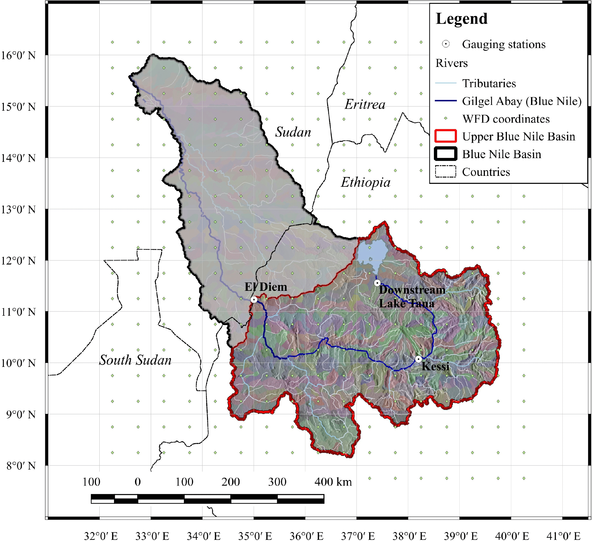
Figure 1Map of the Blue Nile River basin. The Upper Blue Nile (UBN) catchment (172 000 km2) is enclosed by the red line. The three gauges used for model calibration and validation are represented by white circles.
The entire Blue Nile River basin covers an area of about 296 000 km2. The study area considered here is the Upper Blue Nile catchment (UBN) defined at gauge El Diem at the border between Ethiopia and Sudan that covers an area of 172 000 km2. Elshamy et al. (2009) estimates a catchment area of 185 000 km2 and Mengistu and Sorteberg (2012) an area of 174 000 km2 for the UBN. These discrepancies are certainly based on different digital elevation models and GIS algorithms used to delineate the catchment area and thus may add to the uncertainties of such studies, which are not easily quantifiable. In Fig. 1, the UBN is encircled by a red line. In addition, it shows the 576 subbasins that were delineated for the hydrological modelling exercise, the three gauging stations used to calibrate the hydrological model, and the coordinates of the climate data grid. The source of the Blue Nile River is Lake Tana in the Ethiopian highlands and the catchment is located in the north-western part of Ethiopia (Taye and Willems, 2012). It drains a major part of the western highlands (Sutcliffe and Parks, 1999) that is predominantly governed by a unimodal rainfall regime depending on the movement of the intertropical convergence zone (ITCZ). The inter-annual variability of annual rainfall amounts in the Ethiopian highlands is high (Zaitchik et al., 2012) and ranges between 800 and 2200 mm, and the elevation of the UBN varies from 4000 to 500 m.a.s.l. (Taye and Willems, 2012). The river has a length of almost 1000 km from the Lake Tana outlet to the Sudan border.
3.1 Data
Freely available WATCH Forcing Data (WFD) (Weedon et al., 2011) based on ERA-40 (Uppala et al., 2005) reanalysis and climate observations were used to bias-correct five ESMs and 10 RCM runs and to calibrate and validate the hydrological model SWIM (Soil and Water Integrated Model), developed by Krysanova et al. (2005). Although the quality of WFD varies in space (Rust et al., 2015), this gridded product with a spatial resolution of 0.5∘ was used as input because observed climate data were not available for this study. The SRTM digital elevation model (Jarvis et al., 2008) was used to delineate the 576 subbasins and to derive some terrain-specific parameters. Required soil parameters were derived from the Digital Soil Map of the World (FAO et al., 2009) and land use cover data were reclassified from Global Land Cover (GLC2000) (Bartholomé and Belward, 2005). Observed monthly discharge data for model calibration and validation were provided by the Global Runoff Data Centre (GRDC5).
3.2 Hydrological model
The Soil and Water Integrated Model (SWIM), developed by Krysanova et al. (2005), is a semi-distributed, process-based eco-hydrological model that operates at the daily time step. It was developed on the basis of the MATSALU (Krysanova et al., 1989) and SWAT (Arnold et al., 1993) models and is continuously being further developed and adapted to new or specific requirements (Krysanova et al., 2015). Hydrological response units (HRUs), considered as areas with similar hydrological characteristics, are the smallest model units where all hydrological, nutrient, and vegetation processes are calculated. There is no lateral interaction between HRUs but area-weighted daily fluxes are calculated and aggregated at the subbasin scale and routed through the river network. SWIM distinguishes three flow components: surface runoff, subsurface runoff, and contributions of the shallow groundwater aquifer. Actual evapotranspiration is determined by simulated soil evaporation and transpiration from the vegetation cover. Water percolating from the shallow groundwater aquifer into the deep groundwater aquifer is lost from the system but is considered in the water balance.
A reservoir module, developed by Koch et al. (2013), was incorporated in SWIM and parameterized to better account for Lake Tana's storage effects and to consider the impact of the weir at the lake's outlet in future simulations that was constructed in the year 1996.
Radiation data required by SWIM as essential climate input were not available in all RCM runs. To maintain consistency and comparability in hydrological simulations, daily radiation data were computed after Hargreaves and Samani (1985) from daily minimum and maximum air temperature and the latitude of the respective subbasin. The simulated radiation data were calibrated to fit average annual observed radiation data of about 1800 kWh m−2.
3.3 Climate models
The ESM ensemble used in this study consists of the following five CMIP5 models: GFDL-ESM2M, HadGEM2-ES, IPSL-CM5A-LR, MIROC-ESM-CHEM, and NorESM1-M. Projections of these five ESMs were linearly downscaled and bias-corrected by Hempel et al. (2013) in the frame of the Inter-Sectoral Impact Model Intercomparison Project (ISIMIP)6 (Warszawski et al., 2014). The uncorrected ESM simulations were interpolated to the WFD 0.5∘ grid.
Table S1 in the Supplement provides an overview of the RCM runs organized by the CORDEX Africa initiative7. The ensemble consists of four RCMs driven by different ESMs. The RCM SMHI-RCA4 was driven by seven ESMs, CanRCM4 by CanESM2, and the RCMs KNMI-RACMO22T and DMI-HIRHAM4 by EC-EARTH. The 10 RCM runs were bias-corrected by the authors of this paper. Table S2 shows the model IDs of all 15 climate models used in some figures and tables.
3.4 Climate scenarios
For both the global and regional climate model ensembles, the two scenarios RCP 4.5 and RCP 8.5 were used because they represent a broad range of uncertainties with regard to possible future pathways and related climate projections. According to van Vuuren et al. (2011) and Meinshausen et al. (2011), RCP 4.5 represents the medium stabilization scenario (stabilization without overshoot pathway leading to +4.5 W m−2 radiative forcing (relative to pre-industrial forcing) and ∼ 650 ppm CO2 equiv. by 2100) and RCP 8.5 the highest emission scenario (rising radiative forcing pathway leading to +8.5 W m−2 and ∼ 1370 ppm CO2 eq. by 2100), assuming no stabilization in global greenhouse gas emissions.
3.5 Bias correction
Despite regional downscaling to finer resolution, RCM simulations often show considerable biases when compared to observed data (Addor and Seibert, 2014; Christensen et al., 2008). A review of bias correction methods (linear scaling, local intensity scaling, power transformation, and distribution or quantile mapping) is provided by Teutschbein and Seibert (2012). The authors conclude that the distribution or quantile mapping method achieves the best performance for most of the selected criteria. Although quantile mapping is a successful method to improve the representation of daily rainfall characteristics, it fails to correct multi-day and inter-annual variables, such as mean maximum 4-day precipitation, mean minimum 14-day precipitation, and inter-annual variability (Addor and Seibert, 2014). The drawback that all approaches have in common is that they are based on the stationarity assumption, which presumes that future physical processes in the atmosphere are comparable to the period used to correct the simulations. Bias correction of climate simulation data is nowadays a widely used practice in hydrological impact modelling, but it should be treated with caution. As Maraun et al. (2010) point out, the origins of the bias in climate simulations (mathematical formulations in climate models) are not solved by the post-processing and may disrupt internal physical coherence between weather variables. Hence, the correction is usually based on wrong reasons (Addor and Seibert, 2014). Alternatives to bias correction are so-called delta-change methods. Sophisticated approaches of this method are described by Anandhi et al. (2011), Bosshard et al. (2011), and Chiew et al. (2009).
3.5.1 Bias correction of ESMs
Bias-corrected data of five CMIP5 ESMs were available and provided by ISIMIP. In a first step ESM data were linearly interpolated to the WFD 0.5∘ grid, implementing the standard Gregorian calendar. Temperature data were corrected using a trend-preserving additive approach where monthly mean values were adjusted for a systematic bias by adding a grid-point-specific and month-specific constant offset. Therefore, the absolute projected temperature changes of the ESMs are not changed. The daily variability of ESM temperatures was adjusted to reproduce WFD variability by adding a monthly correction factor on temperature anomalies.
Precipitation data were corrected using a multiplicative approach where monthly mean precipitation was multiplied by a grid-point-specific and month-specific constant correction factor. Relative changes projected by the ESMs are thereby preserved. A known problem of this method is that extraordinarily high values of daily precipitation can occur in the bias-corrected simulation if very high simulated daily precipitation data are multiplied by high correction factors. Therefore, the correction factor was limited to a value of 10. Remaining extremely high daily precipitation values were truncated to 400 mm. After the method introduced by Piani et al. (2010), daily precipitation variability and the frequency of dry days were corrected by applying a transfer function to fit the normalized simulated time series of wet months to the normalized WFD time series. A more detailed description of the bias correction procedure applied to the five CMIP5 ESMs used in this study is provided by Hempel et al. (2013).
3.5.2 Bias correction of RCMs
Precipitation biases in most CORDEX RCMs show a high seasonality for grid boxes within the evaluation domain of the UBN. This limits a bias correction based on seasonal or annual means. However, as some of these grid boxes do show almost no precipitation events for single months, a harmonic-based bias correction method analogous to the one applied to temperature is not feasible for precipitation. Furthermore, this results in a large uncertainty in the estimation of the corresponding monthly biases. Thus, based on the recommendation from Dobler and Ahrens (2008), a bias correction is only applied on months and grid boxes with more than 100 rainy days (rainfall above 1 mm day−1) within the calibration period (1951–2001).
The method applied is based on a local rainy day intensity scaling, correcting the frequency of rainy days and the mean precipitation on rainy days to fit the observed values in a specific calibration period (Schmidli et al., 2006). Details on the implementation and an evaluation are given in Dobler and Ahrens (2008). The method has been successfully applied before as a downscaling and bias-correcting method for precipitation in alpine regions (Dobler and Ahrens, 2008; Dobler et al., 2011).
The underlying idea is the assumption of a smooth seasonal cycle for the variables simulated by the RCM and the observational reference (WFD). These cycles are modelled with a series of harmonic functions using vector generalized linear models (Yee, 2015), and the difference in cycles between an RCM reference simulation and the observational product is used for bias correction of the RCM projection.
The seasonality in the location parameter of a quantity (i.e. the expectation value in the case of a Gaussian distribution) can be modelled as
with , being the time variable running over all possible days of the year; K and L are the orders of the harmonic function expansion for μ. A scale parameter σ can be modelled analogously in this framework. The result is a climatological distribution, i.e. a description of the probability distribution throughout the year.
Selection of orders K and L is based on a 10-fold cross validation using the Continuous Rank Probability Score (CRPS, Wilks, 2011) as the cost function. The difference in parameters between the RCM reference and the observational product (WFD) is subtracted from the parameters of the RCM projections for bias correction. Quantile mapping (e.g. Vrac and Friederichs, 2015) now maps the values from the uncorrected to the corrected climatological distribution.
Particular care needs to be taken when correcting minimum and maximum temperature to avoid inconsistencies such as . Here, a variable transformation ensures physical consistency:
After bias-correcting T1 and T2, corrected values for Tmax and Tmin can be obtained by back-transforming the variables.
3.6 Evaluating the suitability of climate simulations
Evaluating the suitability of climate simulations for regional impact studies is a process that includes seemingly objective components (e.g. analysing performance criteria) and subjective components (choosing criteria and setting their thresholds). Data visualization and interpretation by the user might be considered as a mixture of both objectivity and subjectivity. The choice of periods used as reference and future projection does also influence the results. The former is often predetermined by data availability or conventions and the latter usually by the client. Moreover, there are uncertainties with regard to the quality of the dataset used as the comparison baseline, mostly observed and/or generated climate data.
Evaluation of climate model performance is complicated by the fact that climate simulations cannot be compared to the reference dataset on a real-time daily, monthly, or annual basis, as is common practice with discharge simulations in hydrological modelling. Climate simulations are not supposed to reproduce or predict the weather for a certain day, month, or year. Hence, only statistical parameters, summarized over a period of usually 30 years (e.g. the annual cycle represented by average daily or monthly time series), or the mean, quantile values, and standard deviation of the entire daily time series can be used as a basis for comparison.
In the first step of climate model evaluation, daily and monthly precipitation characteristics of uncorrected (UC) and bias-corrected (BC) climate simulations were compared to WFD characteristics (reference climate). In a second step, SWIM was employed to simulate daily discharge using all climate simulations for reference and future periods. Since the main purpose of this study is to assess climate change impacts on hydrology, using hydrological performance indicators to evaluate climate simulations is a straightforward method. A similar approach was used by Elshamy et al. (2013) who used a GLUE-like methodology to exclude and weigh climate model performance. Another benefit of this approach is that a spatially semi-distributed hydrological model does not only account for temporal but also for spatial patterns of climate inputs. Therefore, the annual cycle represented by daily (n=365) discharge simulations (sim), averaged over the 30-year reference period, was compared against the baseline simulation using WFD (ref). The performance criteria applied to these time series are the coefficient of determination (R2), PBIAS, standard deviation (SD), and the normalized SD of discrepancies (SDD) or the centred root mean square errors.
The characteristics of daily discharges were analysed using flow duration curves (FDCs), where every single discharge value is related to the percentage of time it is equalled or exceeded (Smakhtin, 2000). FDCs summarize discharge variability of a time series and display the complete range from low flows to flood events. In order to analyse and visualize average, low, and high flow characteristics, 17 percentile values (Q0.01–Q99.99) were used to compute FDCs based on the entire daily discharge time series of the 30-year reference period. This method was applied to assess whether model performance is suitable to study non-extreme discharge conditions (NED) and/or high and low flow situations as well as their extremes.
In addition to the criteria used to evaluate model performance in the reference period, it is also important to consider model behaviour in future periods. In fact, unexpected behaviour in projection periods was observed in several simulations, particularly in some BC simulations. The hypothesis is that the stronger the necessity of bias correction, the higher the risk that the BC simulation will show unexpected behaviour in future periods. Therefore, another criterion was introduced that indicates the rate of change of PBIAS between the future and the reference period. Note that the definition of threshold values is somewhat subjective and was influenced by the simulation results of the model ensemble. However, if the thresholds had been set more critically, almost no climate model would have passed the evaluation process successfully. The model selection process and the definition of criteria thresholds are described in the following section.
Table 1Selection of uncorrected (UC) and bias-corrected (BC) Earth system models (ESMs) and regional climate models (RCMs).
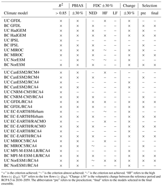
“×” is the criterion achieved; “∼” is the criterion almost achieved; “–” is the criterion not achieved. “HF” refers to the high flows (≤Q10); “LF” refers to the low flows (≥Q90). “Change ±30” is the volumetric change between the reference period and RCP 8.5 in 2030–2059. The abbreviation “pre” refers to the preselection; “final” refers to the models selected in the final ensemble.
3.7 Model selection
Beside analysing the impact of climate projections on future discharges using the whole UC and BC ESM and RCM ensembles, a climate model ensemble was assembled containing only those models that fulfil the criteria and their thresholds defined below. In order to become a member of the selected ensemble, a model must basically achieve all the following three criteria.
-
Seasonality. The annual cycle based on average daily discharge simulations must achieve R2≥0.85. Models with R2<0.85 are assumed to represent discharge seasonality only poorly.
-
Volumetric deviation. Average daily discharge simulations must achieve a %.
-
Non-extreme discharges (NED). NED represent discharge conditions between FDC percentile values between >Q10 and <Q90 (). Percentiles in this range should not deviate more than ±30 % from WFD discharge simulation.
Models meeting these three criteria are assumed to be suitable for a qualitative impact assessment and are indicated in the column ”pre” (preselection) in Table 1. In addition, the columns HF (high flows, FDC percentiles Q10, Q5, Q1, Q0.1, Q0.01) and LF (low flows, FDC percentiles Q90, Q95, Q99, Q99.9, Q99.99) indicate further whether a particular model adequately represents extreme discharge conditions and might be used for specific investigations. Again, the FDC values in the respective range should not exceed the threshold of ±30 %.
After simulating discharges using all climate scenarios it was found that several simulations project enormous increase in annual river discharge already in the period 2030–2059. This was particularly the case in simulations where bias correction resulted in stupendous increase of extreme daily rainfall and therefore extraordinary high peak discharges. Hence, another criterion was defined representing the rate of change. Simulations where average annual discharges changed by more than ±30 % in the period 2030–2059 (RCP 8.5) relative to the reference period were omitted from the selected ensemble, even if the first three criteria were achieved. This criterion is represented in Table 1 in the column ”Change”, which reveals that both UC and BC models either always achieve or do not achieve this criterion.
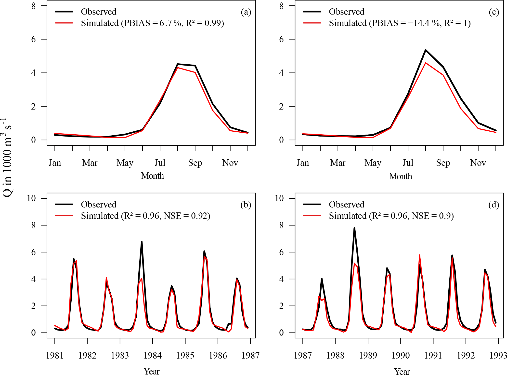
Figure 2Simulated discharges for calibration (a, b) and validation (c, d) periods at gauge El Diem (Sudan border) using WATCH Forcing Data (WFD). The annual cycle is shown in the top row and average monthly discharges in the bottom row.
4.1 Model calibration and validation
The eco-hydrological model SWIM was calibrated to three discharge gauges in the UBN: (1) downstream Lake Tana, (2) Kessie, and (3) El Diem. Due to limited data availability, the model was calibrated to the monthly time step using a semi-automated approach. The calibration (1981–1986) and validation (1987–1992) periods for gauge El Diem were on the one hand chosen according to data availability and on the other hand to cover periods of wet and dry years. Data availability for the gauges Lake Tana and Kessie was limited to the years 1969–1975 and 1976–1979, respectively. The gauges were successively calibrated where a parameter sensitivity analysis was performed in a first step to assess reasonable parameter ranges as boundary conditions for the automatic calibration algorithm PEST (Model-Independent Parameter Estimation & Uncertainty Analysis software)8. The objective functions to measure model performance are the Nash–Sutcliffe efficiency (NSE) (Nash and Sutcliffe, 1970) and PBIAS, where NSE was the primary criterion.
Figure 2 shows the results of monthly and average monthly discharges at gauge El Diem for calibration (left panel) and validation (right panel). According to Moriasi et al. (2007), NSE values of 0.92 (calibration) and 0.90 (validation) are considered to be very good for the monthly time step. The same classification is achieved for the volumetric errors in both periods. The percent bias (PBIAS) between simulated and observed data is −6.7 % (calibration) and −14.4 % (validation). SWIM simulates peak discharges adequately in most years with few exceptions of rather large underestimation in the years 1983, 1987, and 1988. One explanation for this is the lack of accuracy of WFD inputs and/or observed discharge in some years. The simulated amount of water percolating into the deep aquifer is about 7 % on average. Without this recharge component, it was not possible to achieve good simulations during the dry period.
Figure S1a and b in the Supplement show the calibration results for the gauges downstream Lake Tana and Kessie. The available GRDC discharge time series for both gauges are rather short and in the case of Tana, the data of the years 1973–1975 are not reliable. Compared to the discharge data given in Dile et al. (2013) and Setegn et al. (2011), maximum discharges are usually around 200–250 m3 s−1, as is the case in the years 1969–1972 (Fig. S1a). Monthly WFD precipitation volumes do not explain the high discharges observed in the last 3 years. Hence, only the first 4 years were used for calibration, where an NSE of 0.67 and a PBIAS of 23.1 % were achieved. Monthly discharges at gauge Kessie in the four years where GRDC data were available are underestimated by −18.8 % and achieved an NSE of 0.92. According to Moriasi et al. (2007) the results for the two gauges can be classified to be between good and very good.
4.2 Model performance
4.2.1 Performance of daily and monthly precipitation
Monthly medians and average annual precipitation sums of UC ESM and RCM simulations deviate sometimes strongly from WFD (see Figs. S2, S3, and S4 in the Supplement). The underlying data for the box plots are monthly precipitation sums of the 30-year reference period averaged over the UBN catchment area. Bias correction improved the performance of both indicators considerably in both model ensembles. Deviations of average annual precipitation of all BC ESMs are lower than ±2 %. The results for the BC RCM ensemble are more diverse. Five RCMs deviate 2 %, three RCMs 5 %, and two RCMs 7 %.
Despite the improvement of monthly medians and average annual precipitation sums, bias correction increased the range of monthly precipitation sums critically in several models in both ensembles. This phenomenon can be observed particularly if the deviation of monthly medians between UC simulation and WFD is rather large (e.g. IPSL from May to October, MIROC in July, NorESM in July and August). The effect of increasing variability of monthly precipitation sums is even higher with the method used to bias-correct RCMs and is true for all RCMs (Figs. S3 and S4). The extreme outliers in many models generated by both correction methods are also noticeable.
Not all UC models do adequately represent the unimodal rainfall regime in the UBN. UC NorESM shows for instance a distinct bimodal regime, which is also visible but less pronounced in GFDL and MIROC (Fig. S2) and only weakly visible in MIROC/RCA4 (Fig. S4). Although bias correction eliminated this deficiency, it is questionable at what cost. The physical basis was certainly disrupted by the correction method applied.
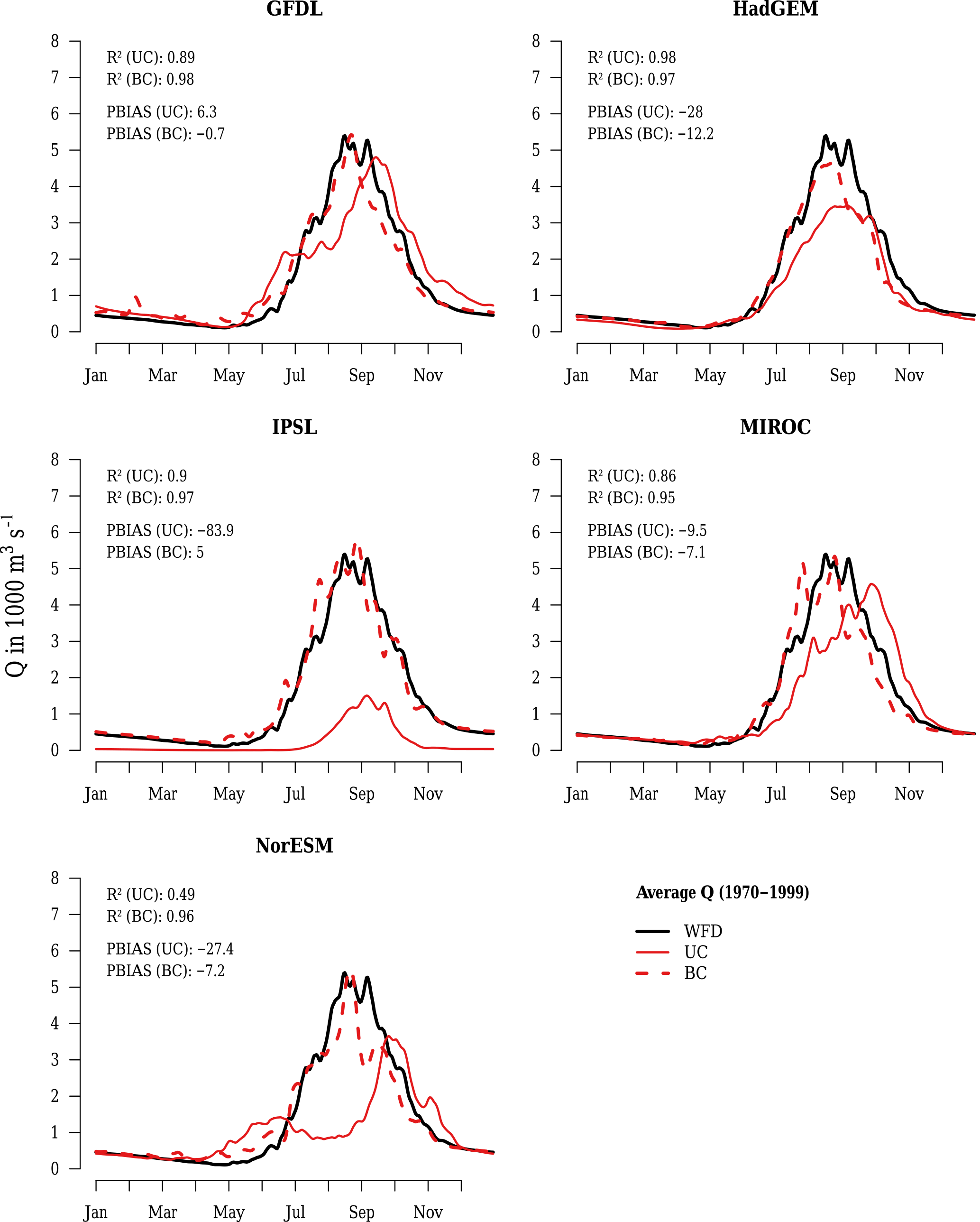
Figure 3Annual cycle of average daily uncorrected (UC) and bias-corrected (BC) simulated discharges at gauge El Diem using Earth system model input and WATCH Forcing Data (WFD) in the reference period (1970–1999).
Tables S3 and S4 in the Supplement show the following statistical parameters of daily precipitation averaged over the catchment: average number of days with precipitation > 1 mm per annum (nDays > 1 mm), average daily precipitation (ave), maximum daily precipitation (max), standard deviation (SD), average precipitation in July, August, and September (ave JAS), and the standard deviation of daily precipitation in July, August, and September (SD JAS). Where Table S3 shows absolute values, Table S4 shows the differences to WFD precipitation (sim-WFD). The two SD parameters were computed by division, SDsim∕SDWFD. The Tables show for instance that maximum daily precipitation is underestimated by all UC models except MIROC. Bias correction resulted in overestimation in 13 out of 15 models. All BC RCMs overestimate maximum daily precipitation, many of them significantly; yet the differences in average daily precipitation of BC simulations are, with exceptions, usually rather small. Large deviations in maximum daily precipitation and in the number of rainy days at the same time, while achieving only small differences in average daily precipitation, indicate that the distribution of daily rainfall can differ sometimes strongly among simulations. It is also noticeable that the SD of daily precipitation of all UC models is lower than the WFD SD. Almost all BC simulations show higher SD than the UC simulations, where all ESM SD values are still lower than WFD SD and all RCM SD values are greater than or equal to WFD SD.
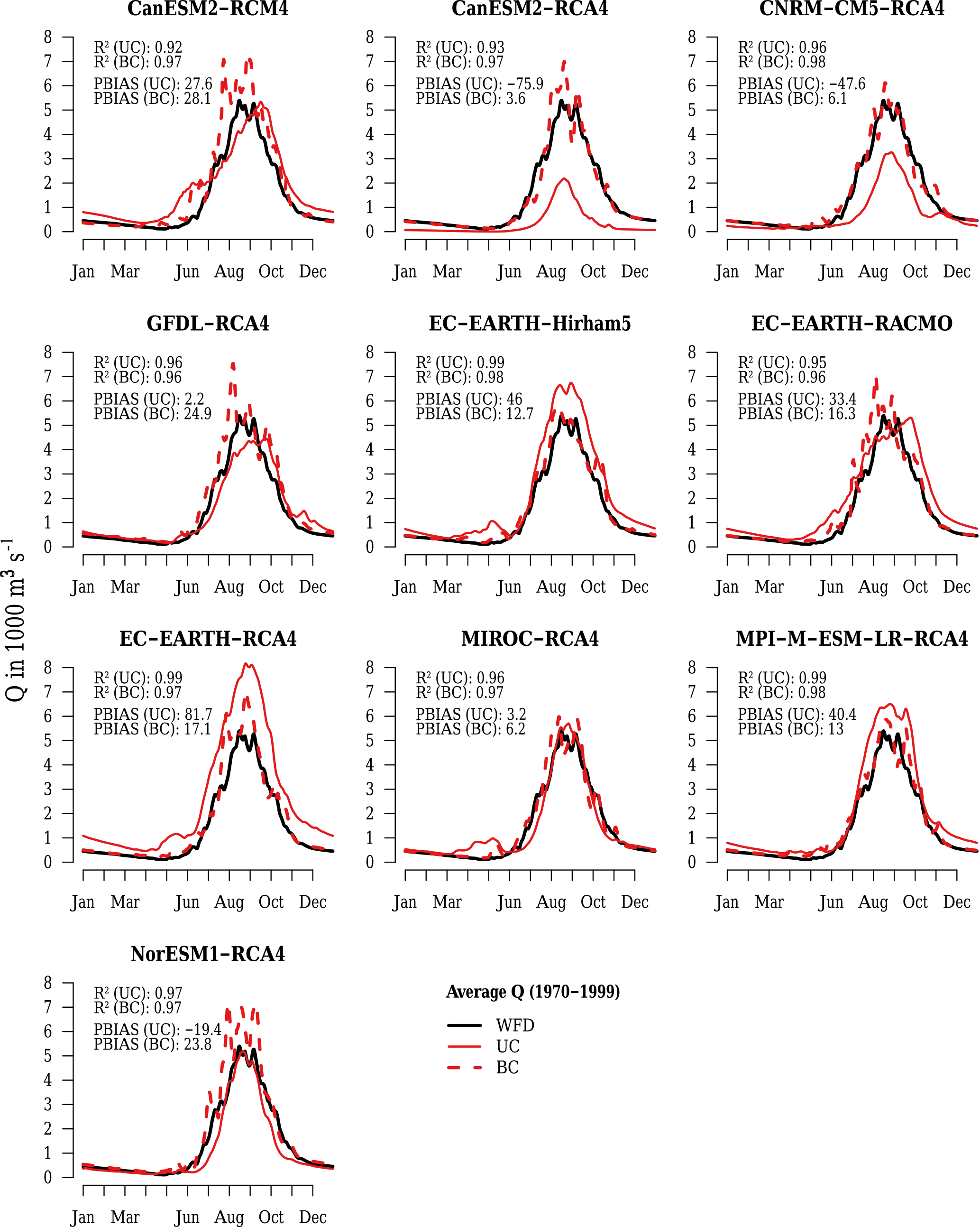
Figure 4Annual cycle of average daily uncorrected (UC) and bias-corrected (BC) simulated discharges at gauge El Diem using regional climate model input and WATCH Forcing Data (WFD) in the reference period (1970–1999).
4.2.2 Performance of average daily discharge using UC and BC climate input
Bias correction improved the performance of averaged daily discharge simulations (n=365) considerably for all members of the ESM ensemble and for most members of the RCM ensemble. Figures 3 and 4 show the simulated hydrographs in the reference period comparing UC and BC simulations with WFD using R2 and PBIAS to indicate discharge performance of the annual cycle.
All UC discharge simulations using ESM climate input, except the one based on GFDL, underestimate average annual discharges, which is indicated by negative PBIAS values (Fig. 3). IPSL shows the largest deviations, with a PBIAS of −84 %. All other models deviate less than 30 % from WFD discharges. R2 values indicate that seasonal discharge patterns are more or less adequately represented by all models, except NorESM, which simulates a bimodal regime with a small peak in June and a high peak in October instead of one single major peak between August and September. Peak discharges simulated with GFDL and MIROC climate input occur approximately 4 weeks later than the peak simulated with WFD. Discharges simulated with HadGEM achieve an R2 of 0.98 but are too low during the high flow season. Another example is the UC IPSL model, which achieves an R2 of 0.9, although it underestimates discharge by −84 %. Hence, high R2 values can be misleading if they are not combined with a volumetric criterion such as PBIAS.
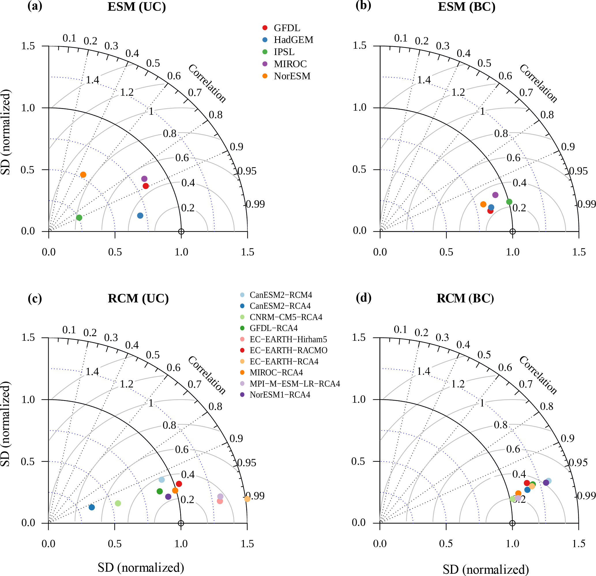
Figure 5Taylor diagram of average daily discharges at gauge El Diem in the reference period (1970–1999). It shows R2, standard deviation (SD) normalized by SDref, and normalized SDD of discrepancies for Earth system model (ESM) input in the top row and regional climate model (RCM) input in the bottom row.
In contrast to ESMs, the majority of discharge simulations based on UC RCMs overestimate average annual discharges in the reference period (Fig. 4). The deviations of six UC RCMs are larger than 30 %. However, seasonal discharge patterns are generally better represented using UC RCM climate input than UC ESM input. The lowest UC RCM R2 value is 0.93 compared to an R2 of 0.49 by NorESM of the UC ESM ensemble. Hence, bias correction improved R2 values only slightly for 50 % of RCMs. In 60 % of the cases, the volumetric deviation (PBIAS) of BC RCMs is significantly lower than in the corresponding UC models. Based on these two indicators, the performance of BC RCM simulations is generally better than UC RCMs. However, there is a strong tendency of peak flow overestimation in six out of ten BC RCMs, which is not captured by R2 and PBIAS. Therefore, a visual assessment of hydrographs is important as well as an analysis of daily discharge characteristics using FDCs (see following section).
Taylor diagrams (Taylor, 2001) are another method to visualize model performance showing three performance indicators (R2, normalized SD, and SDD) in a single plot (see Fig. 5). They facilitate the visual assessment of model performance where outliers can be easily identified. A model with similar statistical characteristics to the reference dataset would be represented by a point at 1.0 on the x-scale and 0.0 on the y-scale. However, interpretation of normalized values is difficult in terms of numerical thresholds, though Fig. 5a identifies UC IPSL and UC NorESM clearly as outliers. IPSL is, for instance, an outlier because it shows deficiencies at representing SD (0.25 where 1.0 would be ideal) and SDD (0.79 where 0.0 would be ideal). UC NorESM performs poorly in terms of all indicators. After bias correction all ESMs show rather good performance (see Fig. 5b). Except BC IPSL, all models have lower SD than WFD. The characteristics of RCMs are different. Half of the UC RCMs' SDs (Fig. 5c) deviate more than ±0.25 from standardized WFD but perform much better in terms of R2. Interestingly, after bias correction (Fig. 5d), all models show a higher SD than WFD, which is consistent with higher SD of daily rainfall as described in the previous section.
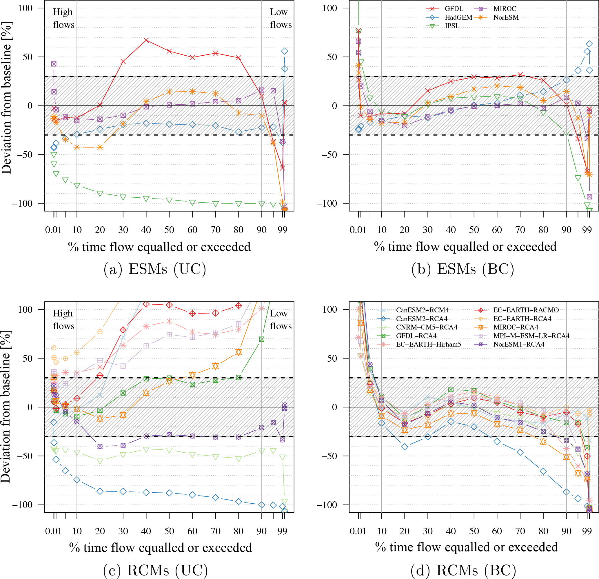
Figure 6Relative deviations of FDCs from baseline discharge simulation at gauge El Diem using WATCH Forcing Data (WFD) in the reference period (1970–1999). Simulations based on uncorrected (UC) and bias-corrected (BC) Earth system model (ESM) input in the top row and regional climate model (RCM) input in the bottom row.
4.2.3 Flow duration curves
FDCs are employed here to analyse and characterize strengths and weaknesses of daily discharge simulations with regard to NED conditions, high flows, low flows, and their extremes. Figure S5 in the Supplement shows FDCs of all ensembles, where the black line represents simulations using WFD. At least one obvious outlier can be clearly identified in both UC ensembles (IPSL and CanESM2-RCA4). Apart from the outliers, NED characteristics are slightly better represented by the UC ESM ensemble (Fig. S5a) than by the UC RCM ensemble (Fig. S5c). Most of the UC RCMs tend to overestimate NED and low flows. At a first glance, the biases were significantly reduced by the correction methods (Fig. S5b and d), especially for NED. However, compared to UC simulations, the correction led to higher biases in the high and low flow segments and especially in their extreme values. Note that a logarithmic y-scale is used where large deviations in the extreme high flow section appear rather small on this plot although they are in fact extremely high.
Figure 6 overcomes this problem by showing relative deviations of FDCs between discharge time series simulated with climate model inputs and the baseline using WFD. The values corresponding to Fig. 6 are provided by Tables S5–S8 in the Supplement. Assuming that deviations in the range of ±30 % are tolerable, there is not a single UC model (Fig. 6a and c) which fulfils these requirements for all percentile values. However, the UC ESMs' MIROC and HadGEM (Fig. 6a) show acceptable deviations (±30 %) in NED conditions, but there is not a single UC RCM representing NED conditions in the given range (Fig. 6c). The best UC RCM result was achieved with NorESM1-RCA4. Figure 6b and d show that bias correction was successful in correcting the biases of NED for all ESMs and seven out of ten RCMs. The correction method applied to ESMs leads to different patterns in the high and low flow sections compared to the method used to bias-correct RCMs.
Between Q1 and Q10 (high flows), the BC ESMs tend to underestimate values (but in the given range of acceptable deviations), whereas BC RCMs overestimate flows corresponding to these percentiles. There is not a single BC RCM that represents Q1 conditions in the given range of ±30 %. The smallest overestimation for Q1 is 52.4 %. All BC RCMs strongly overestimate extreme high flows Q0.1 and Q0.01. The highest Q0.01 overestimation is 656.9 % and the lowest 100.4 % (Table S8). The BC ESMs perform better in the extreme high flow segments. However, only GFDL and HadGEM simulate Q0.1 values in the acceptable range and only HadGEM for Q0.01 (Table S6).
In the low flow section (between Q90 and Q99) there is no BC ESM that performs adequately for all percentile values. Except HadGEM that overestimates low flows, the other models tend to underestimate values. Extreme low flows (Q99.9 and Q99.99) are only represented by GFDL within the acceptable range. The BC RCMs all underestimate low flows, where four models are within the acceptable range of deviations for Q95; there is only one model within this range for Q99 (CanESM2-RCM4). Extreme low flow conditions (Q99.9 and Q99.99) are only represented adequately by EC-EARTH-RCA4; the other RCMs severely underestimate extreme low flows.
To summarize the evaluation of model performance based on FDCs, it can be stated that bias correction improved the performance of simulated NED significantly. However, with a few exceptions, both bias correction methods did not improve the performance of high and low flows. This is particularly true for extreme values, which are strongly exaggerated in most cases.
4.3 Temperature, precipitation, and evapotranspiration projections
Figures 7, 8, and 9 show precipitation, temperature, and actual evapotranspiration projections of the selected model ensemble (Sect. 4.5) for the 21st century for RCP 4.5 and RCP 8.5 as anomalies to the reference period in the UBN. They indicate the total range of change and the 5-year moving average (MA5) for both scenarios. The precipitation MA5 does not show a distinct trend of change over the century, but average annual precipitation is projected to be up to 100 mm (∼ 7 %) higher than in the reference period. The increase is only marginally higher in RCP 8.5 than in RCP 4.5. In Fig. S6 it is shown that a maximum of only three out of 15 UC climate models project decreasing average annual precipitation. The multi-model mean of the CMIP5 ESM ensemble projects showed increasing annual precipitation of 5 % in 2030–2059 and 6 % in 2070–2099 under RCP 4.5 and 8.4 % in 2030–2059 and 15.6 % in 2070–2099 under RCP 8.5. Figure S7 shows where the five ESMs used in this study are situated within the entire CMIP5 ensemble. It is noticeable that only three out of 26 ESMs show declining precipitation trends under RCP 8.5.
Projected surface air temperatures show a clearly increasing trend over the 21st century in both RCPs. Compared to the reference period, the multi-model mean of the selected ensemble projects an increase of 1.7 K (1.5 to 1.9 K) in RCP 4.5 and 2.2 K (1.9 to 3.5 K) in RCP 8.5 in 2050. At the end of the century average temperatures climb up to 2.5 K (1.9 to 4.1 K) under RCP 4.5 and 4.9 K (3.0 to 6.5 K) under RCP 8.5. The multi-model mean of the CMIP5 ESM ensemble projects showed increasing average annual temperatures of 1.6 K in 2030–2059 and 2.3 K in 2070–2099 under RCP 4.5 and 1.7 K in 2030–2059 and 3.9 K in 2070–2099 under RCP 8.5.
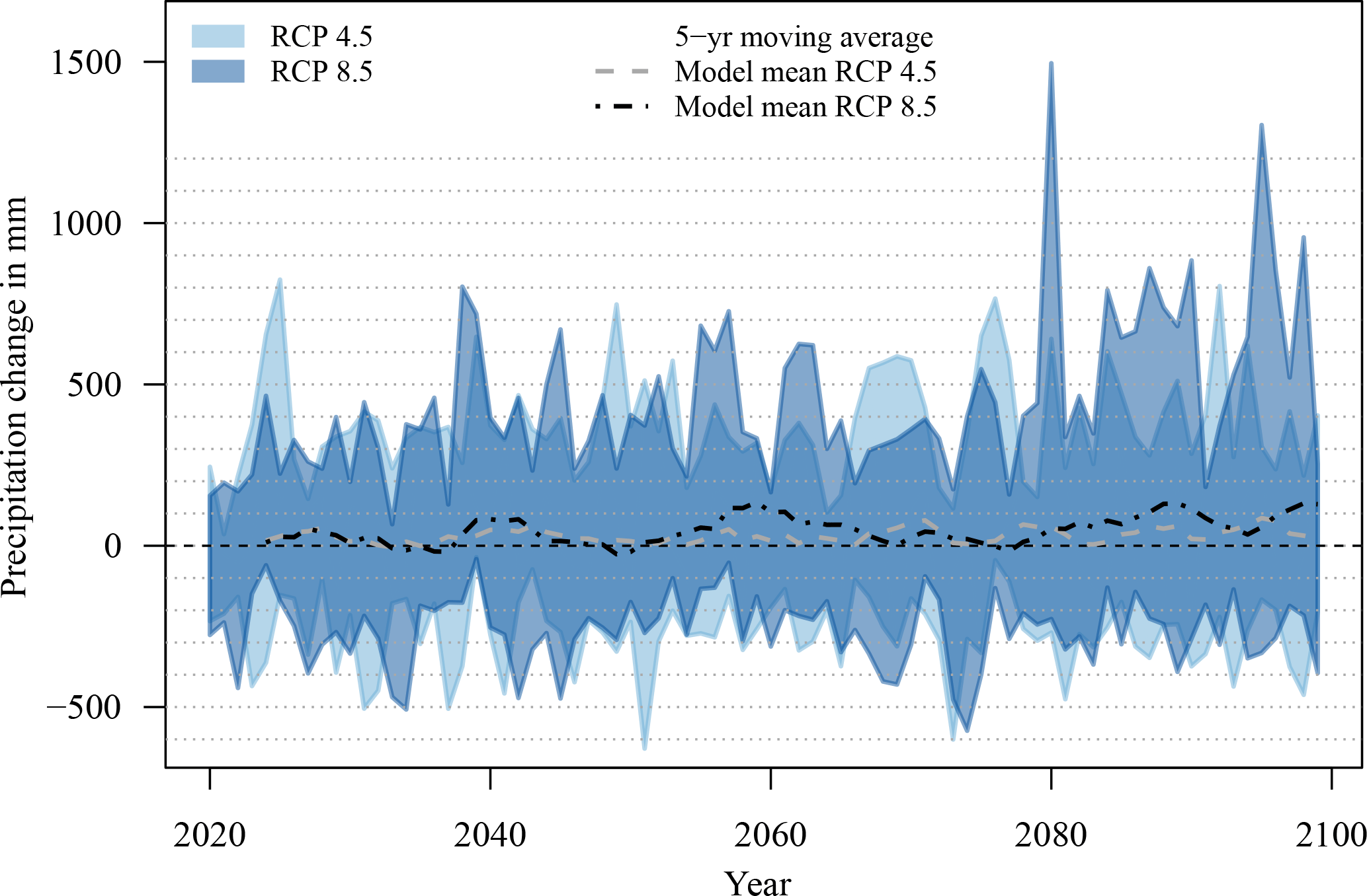
Figure 7Anomalies of annual precipitation amounts relative to the reference period (1970–1999). Range of selected model ensemble.
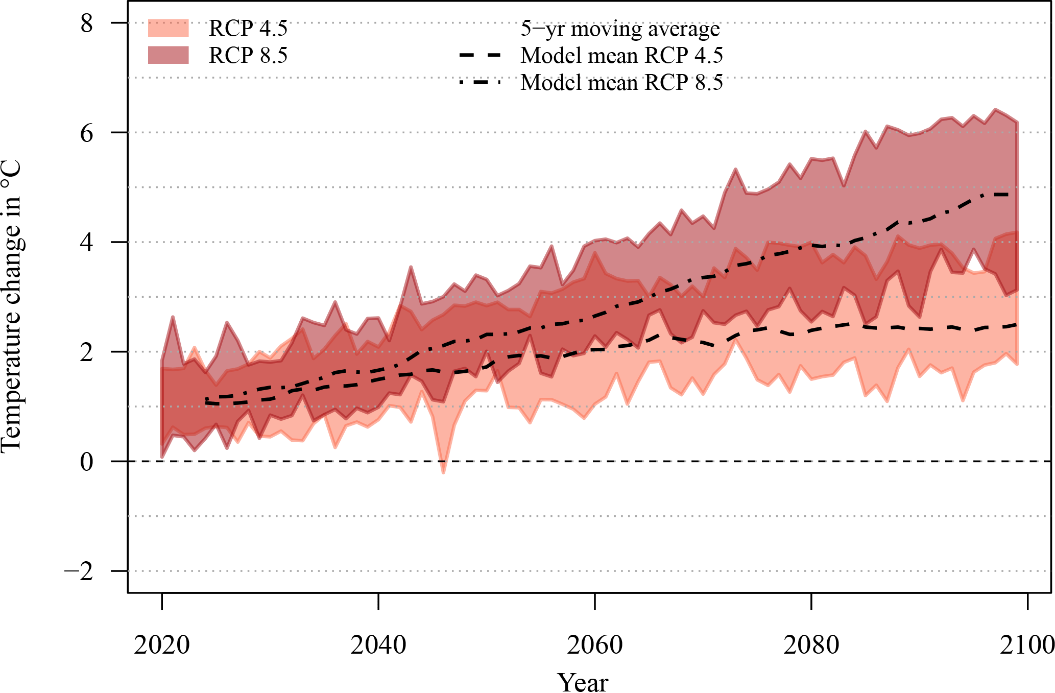
Figure 8Anomalies of average annual mean air temperature relative to the reference period (1970–1999). Range of selected model ensemble.
Although surface air temperature already increases until 2050 in both scenarios by up to 2.2 K, actual evapotranspiration remains rather stable on the level of the reference period. Only in the second half of the 21st century do the projected values increase by up to 50 mm per annum. Hence, it can be concluded that actual evapotranspiration is already at its maximum and can only increase if water availability increases too, as is the case after 2050.
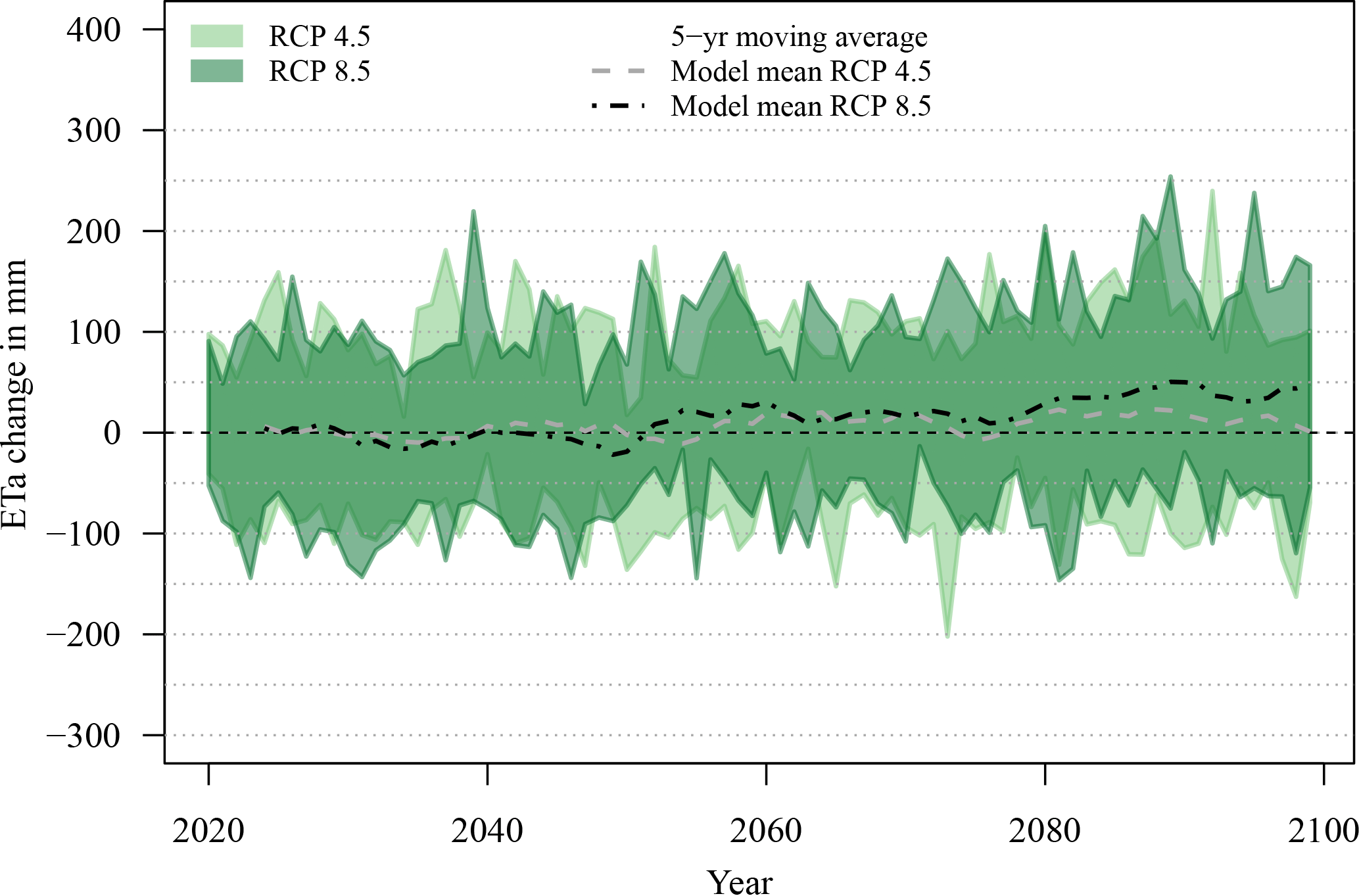
Figure 9Anomalies of annual actual evapotranspiration (ETa) amounts relative to the reference period (1970–1999). Range of selected model ensemble.
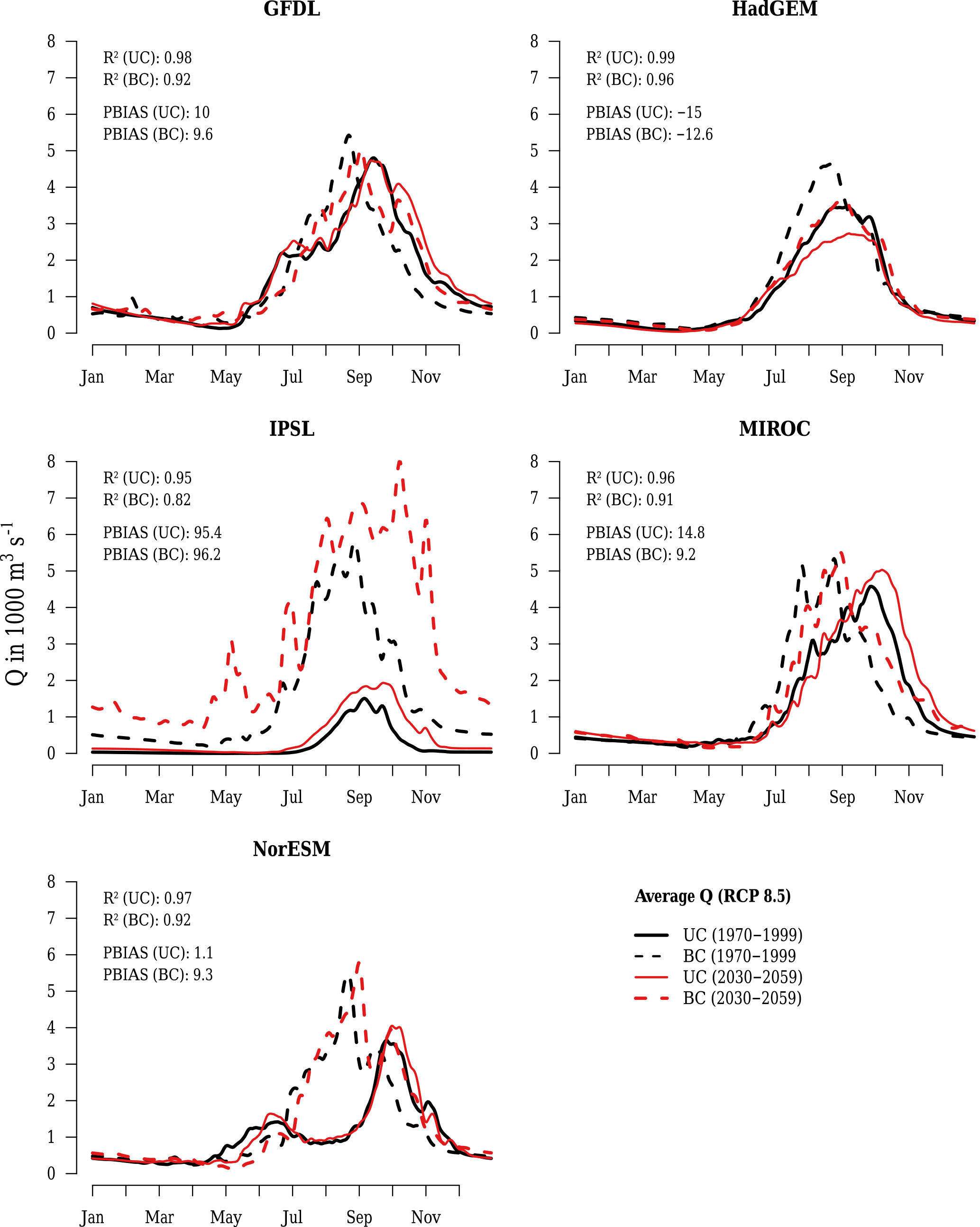
Figure 10Changes of average daily discharges at gauge El Diem based on uncorrected (UC) and bias-corrected (BC) Earth system model (ESM) input in the period (2030–2059) under RCP 8.5 relative to the models' reference period (1970–1999). R2 and PBIAS values are computed to show the differences between the projection period and the reference period.
4.4 Impact of bias correction on discharge projections
Figures 10 and 11 show projected discharge changes of each single model under RCP 8.5 in the period 2030–2059. The changes are relative to the models' reference period. The figures allow the changes between the reference and the future period of UC and BC models to be investigated, as well as the differences of projected changes between UC and BC simulations. The indicators R2 and PBIAS are not used to measure the performance, but they indicate the magnitude of change between the reference and the projection period.
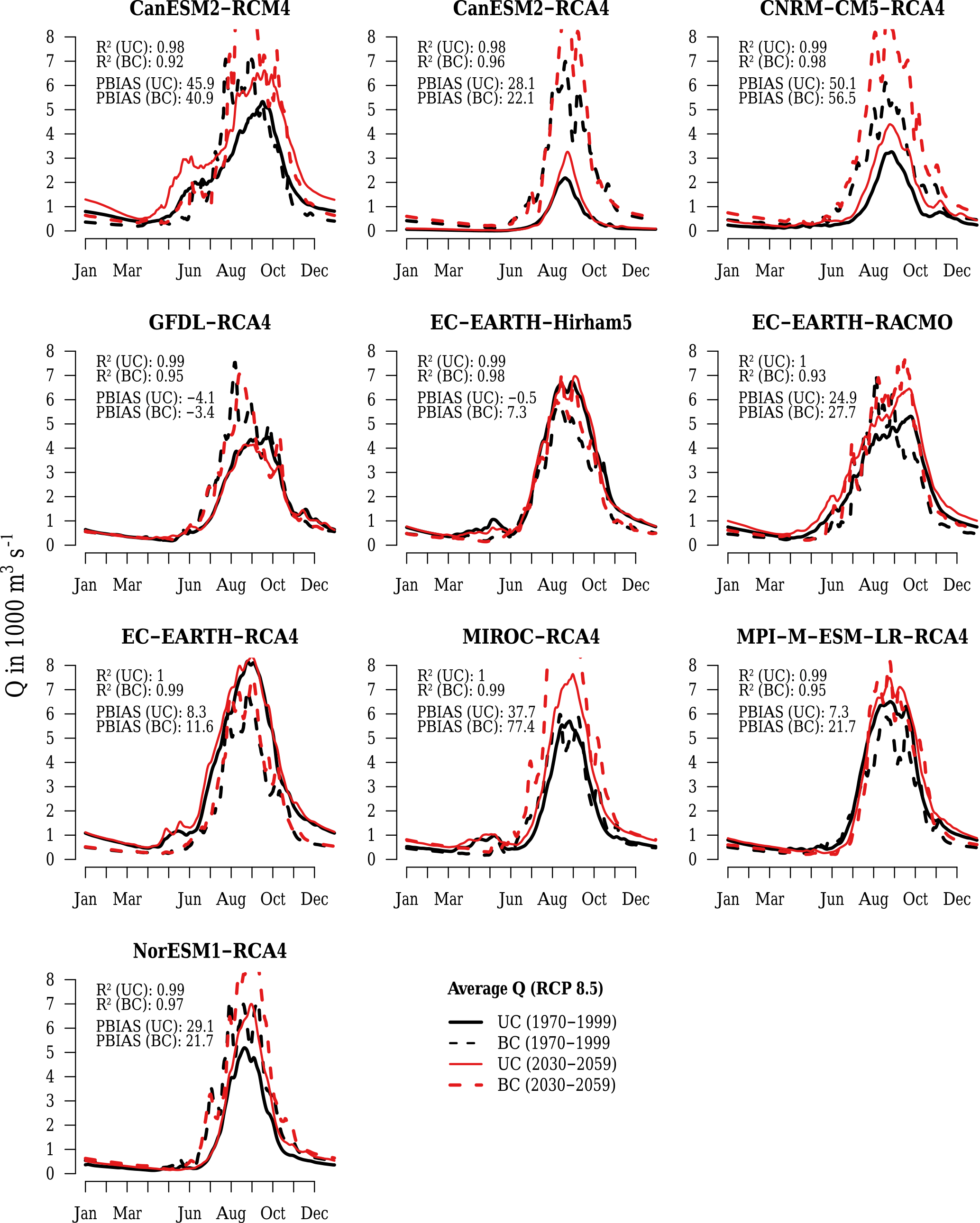
Figure 11Changes of average daily discharges at gauge El Diem based on uncorrected (UC) and bias-corrected (BC) regional climate model (RCM) input in the period (2030–2059) under RCP 8.5 relative to the models' reference period (1970–1999). R2 and PBIAS values are computed to show the differences between the projection period and the reference period.
The IPSL model shows the largest deviations between the future and the reference period (Fig. 10) for both UC and BC simulations. The UC IPSL model projects an increase of 95.4 % in average annual discharge. A visual assessment supports the previously made assumptions that the IPSL model does not provide adequate climate simulations in the study area. This is true for both UC and BC climate simulations. Aich et al. (2014) applied the same five BC ESMs in four large African river basins and found that also in the Niger basin (comparable climate zone to the Blue Nile River) one of the five models projects extreme and unexplainable changes although it performed adequately in the historical period. In the case of the Niger River basin, it was the MIROC model that behaved awkwardly in the projection period, whereas the IPSL behaved normally in the range of the other models.
The HadGEM model is the only model where bias correction changed the sign of the discharge signal. The simulation with UC climate input projects a decrease of average annual discharges of −2.9 % and the BC simulation an increase of +2.2 %. The results of the NorESM1 model are interesting. The UC model simulates a bimodal rainfall and runoff system with a dry period during the rainy season in July to September. Although the model was forced by bias correction into a completely different system, by pushing the dry season into a rainy season, the projections do not seem anywhere near as disrupted as the IPSL simulation. Hence, the NorESM1 results do not support the assumption that strong bias correction necessarily results in unexpected behaviour in future periods. Looking at the change of average peak magnitudes between UC and BC ESM simulations in the reference and the future period, the change signals are in a similar order, except for simulations based on IPSL. They are also in the order of average peaks simulated with WFD input; compare with Fig. 3.
Figure 11 shows that maximal discharge peaks simulated with RCM climate input are often much higher than average peaks simulated with WFD (∼ 6000 m3 s−1). Where only two UC RCMs simulate higher peaks in the reference period (EC-EARTH-Hirham5 and EC-EARTH-RCA4), five BC RCMs simulate peaks higher than 7000 m3 s−1. Looking at projected peaks in the period 2030–2059 (RCP 8.5) shows that nine out of ten BC RCM-driven and five UC RCM simulations simulate peaks that are higher than 7000 m3 s−1. The projected changes of peak discharge magnitudes between UC and BC RCMs are significantly higher in BC simulations in 50 % of the models. This is not surprising because bias correction of RCMs already led to significant overestimation of high flows in the reference period, as was discussed in Sect. 4.2.3. This behaviour is exaggerated in future periods.
4.5 Selected model ensemble
Table 1 summarizes the performance criteria for all UC and BC simulations using R2, PBIAS, deviations from FDC values, and the change rate. The seasonality criterion R2>0.85 was achieved by all simulations except the one based on UC NorESM. Seven out of 30 simulations failed to represent the volumetric deviation criterion PBIAS ± 30 %. Concerning the FDC criteria, 12 simulations passed the NED test, seven simulations the high flow criterion, and only one simulation the low flow criterion. The column ”pre” (preselection) shows whether a model fulfilled the criteria in the first three columns. These models might be chosen for a qualitative impact assessment. However, four models that passed the preselection criteria were omitted from the selected model ensemble because they project very high changes in average annual discharges (column ”Change”). Sometimes both the UC and BC simulations were judged to be suitable. In order not to put too much weight on the results of one model, only the better simulation (UC or BC) was selected for the final model ensemble and is denoted in the column “final”. The latter column indicates that 10 out of 30 simulations passed all performance criteria and thus become members of the selected model ensemble. This ensemble consists of four BC ESMs, four BC RCMs, and two UC RCMs.
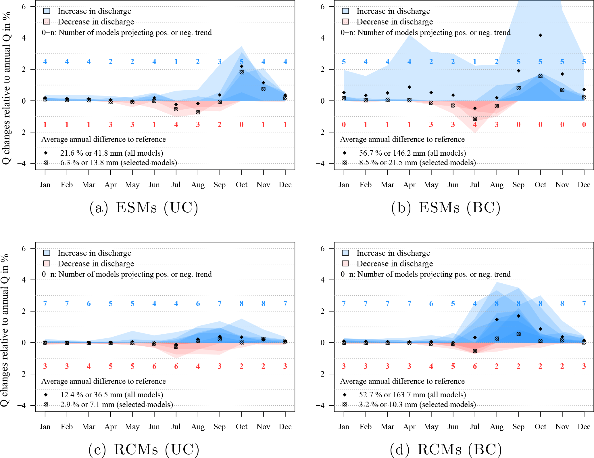
Figure 12Monthly discharge changes of uncorrected (UC) and bias-corrected (BC) Earth system model (ESM) and regional climate model (RCM) simulations in % under RCP 8.5 (2070–2099). Monthly changes are relative to average annual discharge in the reference period (1970–1999) at gauge El Diem.
4.6 Climate impacts on discharges
In this section, the similarities and differences of projected climate change impacts on Blue Nile discharges at gauge El Diem are discussed. The two UC and BC ESM and RCM ensembles and the selected model ensemble are considered (see Table 1, column “final”). In Figs. 12 and 13 and S8–S11, each model simulation is represented by a semi-transparent polygon, where blueish colours indicate an increase and reddish colours a decrease in monthly discharges. The more saturated the colour, the more models project the same rate of change. The figures show monthly changes relative to average annual discharges in the reference period. This method was chosen in order to avoid overemphasizing large relative changes in dry periods which are not significant compared to annual discharges.
Table 2Projected changes in average annual discharges relative to 1970–1999 in %.
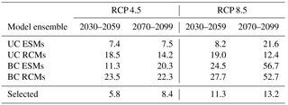
Table 2 shows the total range of changes in average annual discharges projected by the multi-model means of UC and BC ESMs and RCMs and the selected model ensembles. In the near future (2030–2059) in both RCPs, the range of UC models is between 7.4 and 19 %, the range of BC models between 11.3 and 27.7 %, and the range of the selected ensemble between 5.8 and 11.3 %. In the far future (2070–2099) considering both RCPs, the range of UC models is between 7.5 and 21.6 %, the range of BC models between 20.3 and 56.7 %, and the range of the selected ensemble between 8.4 and 13.2 %. The following conclusions summarize the projected changes of average annual discharges more specifically.
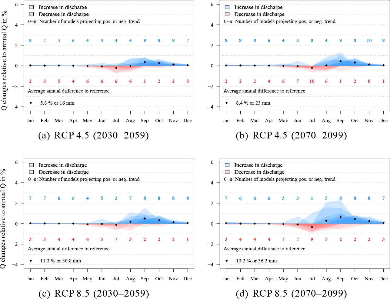
Figure 13Monthly discharge changes of the selected model ensemble (10 models) relative to average annual discharge in the reference period (1970–1999) at gauge El Diem.
-
All ensembles in all RCPs and future periods have in common that they all project an increase of average annual discharges. An exception is the selected model ensemble of the UC ESMs under RCP 4.5 (2030–2059), which projects a decrease of −0.4 % (Fig. S8a).
-
The multi-model means of both UC and BC RCM ensembles (all models) usually project a higher increase of average annual discharges than the ESM ensembles, except under RCP 8.5 (2070–2099); see Figs. S9d and S11d.
-
The multi-model means of BC simulations (both RCPs and periods) always project higher increases in average annual discharges than the UC multi-model means.
-
The magnitude of change signals projected by selected models in the respective ensemble is always lower than the magnitude of the whole ensemble. This is mainly caused by the fact that models projecting changes of 30 %, between the reference period and 2030–2059 under RCP 8.5, were omitted from the ensemble of selected models.
-
A noticeable difference between the UC RCM and ESM ensembles is that projected average annual discharges in the far future are lower (RCMs) and higher (ESMs) than in the near future.
There are also general findings concerning changes in seasonality.
-
There is a trend of decreasing discharges at the end of the dry season projected by all ensembles in both RCPs and periods. The period indicating a drying trend projected by the ESM ensemble tends to be longer and starts a bit earlier (June/July to August) than the trend projected by RCMs (only July).
-
There is a trend of increasing discharges during the rainy season projected by all ensembles in both RCPs and periods. The period indicating higher discharges starts earlier in the RCM ensembles (August to November) than in the ESM ensembles (September to November).
-
Both ensembles agree that there is almost no change projected in the dry period between December and May.
Are we using the right fuel to drive hydrological models? What are the likely impacts of climate change on future discharges in the UBN and is there a strong agreement of projected trends? How far does bias correction influence the results and can we trust models that require strong correction? These questions, posed in the introduction, are discussed in the following.
The majority (≥ 80 %) of the 15 climate models used in this study agree that average annual discharges in the UBN are likely to increase in future. The models project a trend towards decreasing discharges at the end of the dry period (June and July) and an increase during the rainy season (August to November). Due to the use of different climate model ensembles, downscaling approaches, study areas within the UBN, and periods of analysis, a direct comparison with other studies is difficult but clearly reveals that the selection of climate models predominantly influences the results and conclusions made. Setegn et al. (2011) found for instance that the CMIP3 GCMs they used to investigate climate impacts on discharges in the Lake Tana catchment (Blue Nile headwaters) project decreasing trends, but they also state that “…it seems that, by chance, the nine GCMs used in this study are those that show a precipitation decrease…”. On the other hand, Dile et al. (2013) conclude that discharges may increase by up to 135 % in the same region. Taking the, sometimes contradicting, results of recent studies into account (Teklesadik et al., 2017; Dile et al., 2013; Mengistu and Sorteberg, 2012; McCartney and Menker Girma, 2012; Setegn et al., 2011; Conway and Schipper, 2011; Diro et al., 2011; Elshamy et al., 2009), one can conclude that climate impacts in the UBN are uncertain but there is a bias towards a wetter future. The findings of this study, using the most recent global and regional climate models as well as precipitation projections of the entire CMIP5 ensemble, underline the latter statement.
Apart from discussing whether the future in the UBN will become generally wetter or drier, decisions with regard to the adaptation of land and water management to changing climatic conditions requires not only information on qualitative but also accurate seasonal quantitative changes. The value of using uncorrected climate simulations to answer those questions is, due to the lack of spatio-temporal accuracy and the lack of statistically representative observed weather characteristics, usually rather limited. Bias correction of climate simulations is an attempt to overcome at least some of these deficiencies.
The reference dataset used to bias-correct climate models and to calibrate and validate the hydrological model is another source of uncertainty. WFD were used in this study because bias correction on ESMs, provided by ISIMIP, was performed on the basis of this dataset. Moreover, WFD provide a sound basis as climate input, particularly in data-scarce regions, as was shown in various studies (Vetter et al., 2015; Aich et al., 2014; Liersch et al., 2013). The use of a different reference dataset would certainly require different calibration parameter settings and correction factors but would probably not impact the change signals. The most important issue in this connection is the consistency in using the same reference for calibration, validation, and bias correction.
As was shown in this study, monthly medians and average annual precipitation amounts of UC ESM and RCM simulations deviate sometimes strongly from reference climate. Although bias correction improved the performance of average climate conditions, the range of monthly precipitation amounts increased critically in several models, producing some extreme outliers in both ensembles. This phenomenon was particularly observed in simulations where deviations of monthly medians between UC simulations and WFD were rather large in the reference period. Average daily precipitation and the number of rainy days were considerably improved by bias correction, but 13 out of 15 BC models overestimate daily precipitation maxima, and many of them significantly. Hence, the bias correction methods applied to ESMs and RCMs in this study could be considered to be only partly successful. While achieving significant improvement in terms of average daily, monthly, and annual precipitation characteristics, increasing variability of precipitation amounts, and therefore under- and overestimation of extremes, was the result in many simulations.
This phenomenon is problematic for impact studies and the application of hydrological models, particularly if changes of extreme values are the subject of investigation. Large overestimation of precipitation on some days or in some months, for instance, which are balanced by dry months in the long term, can lead to large amounts of excess water that may be simulated almost entirely as surface runoff by the hydrological model. Therefore, it is reasonable to use hydrological performance indicators to evaluate the suitability of climate simulations, particularly for quantitative impact studies, and to create a subset of models for the impact assessment. Another way to deal with low performance in the simulation of extremes in impact studies is to analyse changes in return periods of extreme events (Hattermann et al., 2016).
Due to the fact that discharge simulations, based on climate simulations, cannot be compared to observed discharges on a real-time daily, monthly, or annual basis, the methods to evaluate discharge performance are limited. In this study, the annual cycle (daily time series averaged over the simulation period) was characterized by R2 and PBIAS, where R2 was a measure of seasonality and PBIAS a measure of volumetric deviations. Flow duration curves (FDCs) were used to characterize the distribution of average flow conditions, high and low flows, as well as their extremes, by using the whole time series of daily discharge simulations. Unsurprisingly, discharge simulations show similar deficiencies to precipitation simulations. Using bias-corrected climate simulations improved the performance of non-extreme discharges (NED) significantly but, with few exceptions, the performance of high and low flows did not improve; in fact, it worsened in most of the simulations. Many BC discharge simulations tend to exaggerate high (overestimation) and low flows (underestimation). Comparing peak discharges using UC and BC climate input, for instance, showed a tremendous increase in some BC simulations, although average monthly precipitation patterns of BC models achieved a much better fit than their UC counterparts. Moreover, the multi-model means of BC simulations (both RCPs and periods) always project higher increases in average annual discharges than the UC multi-model means. However, a hydrological impact study in the Danube River basin showed in turn that relative changes in average monthly discharges projected using UC and BC climate models are overall comparable (Stagl and Hattermann, 2015).
Knowing these limitations, one should carefully consider the model's suitability and the purpose it is being used for. An impact study focusing on relative changes of future water availability may have lower requirements in terms of model accuracy than a study with the aim of investigating future extremes, such as floods and droughts or a study addressing land and water management issues including irrigation and/or reservoir operations. Whenever complex water management is involved, bias correction is often unavoidable because the simulation of reservoir and irrigation operations requires rather accurate hydrological input. However, to simply trust in climate input only because it was bias-corrected would be naive. Therefore, the question of model selection is valid. Why should one use or trust models to assess changes in seasonal patterns, for instance, that have not represented those patterns in the past or use a model to investigate future flood risk that completely fails to represent rainfall extremes? Again, bias correction may help to overcome some quality issues but it was also found in this study that improving climate simulations in the reference period does not guarantee higher quality or reliability in simulating future periods. On the contrary, the greater the necessity to correct a particular model, the higher the risk that BC simulations will show unexpected behaviour in future periods, where exceptions confirm the rule. Examples confirming this assumption are the following models: IPSL, CanESM2-RCA4, CNRM-CM5-RCA4, and MIROC-RCA4. However, the NorESM1 model is an exception here, because the BC simulation does not show extreme changes in future periods although strong bias correction was necessary in some months to force the model from a bimodal into a unimodal rainfall regime. It should be emphasized that the analysis of climate model performance in this study is only valid for the region of the UBN. It does not imply that a model which performed poorly in this study area will generally perform poorly in other regions, too.
The authors of this study conclude that a purpose-driven selection of a climate model subset is a reasonable approach, particularly in a regional context. To identify models that perform to a good level, the selection process should include an analysis of climate inputs, seasonal discharge patterns, volumetric deviations, and daily dynamics (FDCs), and an assessment of the magnitude of projected future changes. It is also worth mentioning that the thresholds defined to evaluate model performance have a subjective component and are based on statistical parameters, graphical data interpretation, and modelling expertise. If the thresholds had been set more critically in this study, almost no climate model would have passed the evaluation process successfully. The rather weak thresholds were a compromise and reveal the fact that the performance of many climate models is still far beyond being adequate for applied quantitative impact studies. This statement includes bias-corrected simulations and implies that the ability of bias correction can, depending on the approach, be rather limited and thus does not necessarily improve the reliability per se. In another river basin with different characteristics, e.g. with a nival regime or a bimodal rainfall regime, the performance criteria and their thresholds may have been defined differently. Hence, the model selection method can be applied to other river basins but it is always necessary to consider region-specific characteristics that may require the introduction of new criteria adapted to the situation at hand. However, model selection for regional impact studies is only a reasonable, justifiable, and recommended approach if the uncertainties of the selected ensemble are communicated within the context of the whole model ensemble.
This study demonstrated that neither the trend-preserving method applied to the five ESMs nor the harmonic-based method used to bias-correct the 10 RCMs was able to generate fully satisfactory climate inputs for a regional hydrological impact study with high demands in terms of quantitative accuracy. Hence, further research is required to improve regional climate simulations and/or to investigate alternative correction methods or approaches to make climate simulations meaningful for application-oriented regional studies available. Currently, the most promising solutions seem to be sophisticated delta-change methods, as suggested by Anandhi et al. (2011), Bosshard et al. (2011), and Chiew et al. (2009).
All input data used to set up, calibrate, and validate the hydrological model and to bias correct the global and regional climate simulations are freely available and the corresponding sources are provided in Sect. 3.1. All discharge simulations produced in this study have been made available at https://doi.org/10.4121/uuid:05b9f40f-583d-479b-a79e-f961f72436db (Liersch, 2018). The bias corrected CORDEX simulations are available here: https://doi.org/10.5880/PIK.2018.009 (Liersch et al., 2018).
The supplement related to this article is available online at: https://doi.org/10.5194/hess-22-2163-2018-supplement.
The authors declare that they have no conflict of interest.
This research was funded by the German Federal Foreign Office and supported
by the Ethiopian Environmental Protection Authority and the German Embassy in
Addis Ababa. In addition we thank the two anonymous reviewers for their
constructive comments which helped us to improve the quality of the
manuscript.
Edited by: Ralf Merz
Reviewed by: two
anonymous referees
Abdo, K. S., Fiseha, B. M., Rientjes, T. H. M., Gieske, A. S. M., and Haile, A. T.: Assessment of climate change impacts on the hydrology of Gilgel Abay catchment in Lake Tana basin, Ethiopia, Hydrol. Process., 23, 3661–3669, https://doi.org/10.1002/hyp.7363, 2009. a
Addor, N. and Seibert, J.: Bias correction for hydrological impact studies – beyond the daily perspective, Hydrol. Process., 28, 4823–4828, https://doi.org/10.1002/hyp.10238, 2014. a, b, c, d
Aich, V., Liersch, S., Vetter, T., Huang, S., Tecklenburg, J., Hoffmann, P., Koch, H., Fournet, S., Krysanova, V., Müller, E. N., and Hattermann, F. F.: Comparing impacts of climate change on streamflow in four large African river basins, Hydrol. Earth Syst. Sci., 18, 1305–1321, https://doi.org/10.5194/hess-18-1305-2014, 2014. a, b, c
Anandhi, A., Frei, A., Pierson, D. C., Schneiderman, E. M., Zion, M. S., Lounsbury, D., and Matonse, A. H.: Examination of change factor methodologies for climate change impact assessment, Water Resour. Res., 47, https://doi.org/10.1029/2010WR009104, 2011. a, b
Arnold, J., Allen, P., and Bernhardt, G.: A comprehensive surface groundwater flow model, J. Hydrol., 142, 47–69, 1993. a
Bartholomé, E. and Belward, A.: GLC2000: a new approach to global land cover mapping from Earth observation data, Int. J. Remote Sens., 26, 1959–1977, https://doi.org/10.1080/01431160412331291297, 2005. a
Berg, P., Feldmann, H., and Panitz, H.-J.: Bias correction of high resolution regional climate model data, J. Hydrol., 448–449, 80–92, https://doi.org/10.1016/j.jhydrol.2012.04.026, 2012. a
Beyene, T., Lettenmaier, D., and Kabat, P.: Hydrologic impacts of climate change on the Nile River Basin: implications of the 2007 IPCC scenarios, Climatic Change, 100, 433–461, https://doi.org/10.1007/s10584-009-9693-0, 2010. a, b
Bosshard, T., Kotlarski, S., Ewen, T., and Schär, C.: Spectral representation of the annual cycle in the climate change signal, Hydrol. Earth Syst. Sci., 15, 2777–2788, https://doi.org/10.5194/hess-15-2777-2011, 2011. a, b
Bryan, E., Deressa, T. T., Gbetibouo, G. A., and Ringler, C.: Adaptation to climate change in Ethiopia and South Africa: options and constraints, Environ. Sci. Policy, 12, 413–426, https://doi.org/10.1016/j.envsci.2008.11.002, 2009. a
Busby, J., Cook, K., Vizy, E., Smith, T., and Bekalo, M.: Identifying hot spots of security vulnerability associated with climate change in Africa, Climatic Change, 124, 717–731, https://doi.org/10.1007/s10584-014-1142-z, 2014. a
Chiew, F. H. S., Teng, J., Vaze, J., Post, D. A., Perraud, J. M., Kirono, D. G. C., and Viney, N. R.: Estimating climate change impact on runoff across southeast Australia: Method, results, and implications of the modeling method, Water Resour. Res., 45, W10414, https://doi.org/10.1029/2008WR007338, 2009. a, b
Christensen, J. H., Boberg, F., Christensen, O. B., and Lucas-Picher, P.: On the need for bias correction of regional climate change projections of temperature and precipitation, Geophys. Res. Lett., 35, L20709, https://doi.org/10.1029/2008GL035694, 2008. a
Conway, D. and Hulme, M.: Recent fluctuations in precipitation and runoff over the Nile sub-basins and their impact on main Nile discharge, Climatic Change, 25, 127–151, https://doi.org/10.1007/BF01661202, 1993. a
Conway, D. and Schipper, E. L. F.: Adaptation to climate change in Africa: Challenges and opportunities identified from Ethiopia, Global Environ. Change, 21, 227–237, https://doi.org/10.1016/j.gloenvcha.2010.07.013, 2011. a, b, c
Deressa, T. T., Hassan, R. M., and Ringler, C.: Perception of and adaptation to climate change by farmers in the Nile basin of Ethiopia, J. Agr. Sci., 149, 23–31, https://doi.org/10.1017/S0021859610000687, 2011. a
Di Baldassarre, G., Elshamy, M., van Griensven, A., Soliman, E., Kigobe, M., Ndomba, P., Mutemi, J., Mutua, F., Moges, S., Xuan, Y., Solomatine, D., and Uhlenbrook, S.: Future hydrology and climate in the River Nile basin: a review, Hydrolog. Sci. J., 56, 199–211, https://doi.org/10.1080/02626667.2011.557378, 2011. a
Dile, Y. T., Berndtsson, R., and Setegn, S. G.: Hydrological Response to Climate Change for Gilgel Abay River, in the Lake Tana Basin – Upper Blue Nile Basin of Ethiopia, PLOS ONE, 8, https://doi.org/10.1371/journal.pone.0079296, 2013. a, b, c, d
Diro, G. T., Grimes, D. I. F., Black, E., O'Neill, A., and Pardo-Iguzquiza, E.: Evaluation of reanalysis rainfall estimates over Ethiopia, Int. J. Climatol., 29, 67–78, https://doi.org/10.1002/joc.1699, 2009. a
Diro, G. T., Toniazzo, T., and Shaffrey, L.: Ethiopian Rainfall in Climate Models, in: African Climate and Climate Change, edited by: Williams, C. J. R. and Kniveton, D. R., Vol. 43 of Advances in Global Change Research, 51–69, Springer Netherlands, https://doi.org/10.1007/978-90-481-3842-5_3, 2011. a, b
Dobler, A. and Ahrens, B.: Precipitation by a regional climate model and bias correction in Europe and South Asia, Meteorol. Z., 17, 499–509, 2008. a, b, c
Dobler, A., Yaoming, M., Sharma, N., Kienberger, S., and Ahrens, B.: Regional climate projections in two alpine river basins: Upper Danube and Upper Brahmaputra, Adv. Sci. Res., 7, 11–20, https://doi.org/10.5194/asr-7-11-2011, 2011. a
Dosio, A. and Paruolo, P.: Bias correction of the ENSEMBLES high-resolution climate change projections for use by impact models: Evaluation on the present climate, J. Geophys. Res.-Atmos., 116, D16106, https://doi.org/10.1029/2011JD015934, 2011. a
Elshamy, M., di Baldassarre, G., and van Griensven, A.: Characterizing Climate Model Uncertainty Using an Informal Bayesian Framework: Application to the River Nile, J. Hydrol. Eng. ASCE, 18, 582–589, https://doi.org/10.1061/(ASCE)HE.1943-5584.0000656, 2013. a
Elshamy, M. E., Seierstad, I. A., and Sorteberg, A.: Impacts of climate change on Blue Nile flows using bias-corrected GCM scenarios, Hydrol. Earth Syst. Sci., 13, 551–565, https://doi.org/10.5194/hess-13-551-2009, 2009. a, b, c, d
FAO, IIASA, ISRIC, ISSCAS, and JRC: Harmonized World Soil Database (version 1.1), FAO, Rome, Italy and IIASA, Laxenburg, Austria, 2009. a
Gebreluel, G.: Ethiopia's Grand Renaissance Dam: Ending Africa's Oldest Geopolitical Rivalry?, Wash. Quart., 37, 25–37, https://doi.org/10.1080/0163660X.2014.926207, 2014. a, b
Gudmundsson, L., Bremnes, J. B., Haugen, J. E., and Engen-Skaugen, T.: Technical Note: Downscaling RCM precipitation to the station scale using statistical transformations – a comparison of methods, Hydrol. Earth Syst. Sci., 16, 3383–3390, https://doi.org/10.5194/hess-16-3383-2012, 2012. a
Hagemann, S., Chen, C., Haerter, J. O., Heinke, J., Gerten, D., and Piani, C.: Impact of a Statistical Bias Correction on the Projected Hydrological Changes Obtained from Three GCMs and Two Hydrology Models, J. Hydrometeorol., 12, 556–578, https://doi.org/10.1175/2011JHM1336.1, 2011. a
Hargreaves, G. and Samani, Z.: Reference crop evapotranspiration from temperature, T. ASAE, 11, 96–99, 1985. a
Hattermann, F. F., Huang, S., Burghoff, O., Hoffmann, P., and Kundzewicz, Z. W.: Brief Communication: An update of the article “Modelling flood damages under climate change conditions – a case study for Germany”, Nat. Hazards Earth Syst. Sci., 16, 1617–1622, https://doi.org/10.5194/nhess-16-1617-2016, 2016. a
Headey, D., Taffesse, A. S., and You, L.: Diversification and Development in Pastoralist Ethiopia, World Dev., 56, 200–213, https://doi.org/10.1016/j.worlddev.2013.10.015, 2014. a
Hempel, S., Frieler, K., Warszawski, L., Schewe, J., and Piontek, F.: A trend-preserving bias correction – the ISI-MIP approach, Earth Syst. Dynam., 4, 219–236, https://doi.org/10.5194/esd-4-219-2013, 2013. a, b
Ibrahim, A.: The Nile Basin Cooperative Framework Agreement: The Beginning of the End of Egyptian Hydro-Political Hegemony, Missouri Environmental Law and Policy Review, 18, 284–312, available at: https://scholarship.law.missouri.edu/cgi/viewcontent.cgi?article=1395&context=jesl (last access: 24 January 2018), 2012. a
IPCC: Climate Change 2013. The Physical Science Basis. Working Group I Contribution to the Fifth Assessment Report of the Intergovernmental Panel on Climate Change, Tech. rep., IPCC, available at: http://www.ipcc.ch/report/ar5/wg1/ (last access: 14 April 2016), 2013. a
Jarvis, A., Reuter, H., Nelson, A., and Guevara, E.: Hole-filled seamless SRTM data V4, International Centre for Tropical Agriculture (CIAT), available at: http://srtm.csi.cgiar.org (last access: 9 February 2016), 2008. a
Jeuland, M. and Whittington, D.: Water resources planning under climate change: Assessing the robustness of real options for the Blue Nile, Water Resour. Res., 50, 2086–2107, https://doi.org/10.1002/2013WR013705, 2014. a
Kim, U., Kaluarachchi, J. J., and Smakhtin, V. U.: Climate Change Impacts on Hydrology and Water Resources of the Upper Blue Nile River Basin, Ethiopia, Research Report 126, IWMI, 2008. a, b, c
King, A.: An Assessment of Reservoir Filling Policies under a Changing Climate for Ethiopias Grand Renaissance Dam, PhD thesis, Drexel University, 2013. a
Koch, H., Liersch, S., and Hattermann, F.: Integrating water resources management in eco-hydrological modelling, Water Sci. Technol., 67, 1525–1533, https://doi.org/10.2166/wst.2013.022, 2013. a
Krysanova, V., Meiner, A., Roosaare, J., and Vasilyev, A.: Simulation modelling of the coastal waters pollution from agricultural watershed, Ecol. Model., 49, 7–29, 1989. a
Krysanova, V., Hattermann, F., and Wechsung, F.: Development of the ecohydrological model SWIM for regional impact studies and vulnerability assessment, Hydrol. Process., 19, 763–783, https://doi.org/10.1002/hyp.5619, 2005. a, b
Krysanova, V., Hattermann, F., Huang, S., Hesse, C., Vetter, T., Liersch, S., Koch, H., and Kundzewicz, Z. W.: Modelling climate and land use change impacts with SWIM: lessons learnt from multiple applications, Hydrolog. Sci. J., 60, 606–635, https://doi.org/10.1080/02626667.2014.925560, 2015. a
Liersch, S.: Discharge simulations for the Blue Nile at gauge El Diem based on uncorrected and bias-corrected GCM and RCM inputs, Potsdam Institute for Climate Impact Research, Dataset, https://doi.org/10.4121/uuid:05b9f40f-583d-479b-a79e-f961f72436db, 2018. a
Liersch, S., Cools, J., Kone, B., Koch, H., Diallo, M., Aich, V., Fournet, S., and Hattermann, F.: Vulnerability of food production in the Inner Niger Delta to water resources management under climate variability and change, Environ. Sci. Policy, 34, 18–33, https://doi.org/10.1016/j.envsci.2012.10.014, 2013. a
Liersch, S., Koch, H., and Hattermann, F. F.: Management Scenarios of the Grand Ethiopian Renaissance Dam and Their Impacts under Recent and Future Climates, Water, 9, 728, https://doi.org/10.3390/w9100728, 2017. a, b
Liersch, S., Rust, H., Dobler, A., Kruschke, T., and Fischer, M.: Bias-corrected CORDEX precipitation, min/mean/max temperature for Ethiopia, RCP 4.5 and RCP 8.5, GFZ Data Services, https://doi.org/10.5880/PIK.2018.009, 2018. a
Maraun, D., Wetterhall, F., Ireson, A. M., Chandler, R. E., Kendon, E. J., Widmann, M., Brienen, S., Rust, H. W., Sauter, T., Themeßl, M., Venema, V. K. C., Chun, K. P., Goodess, C. M., Jones, R. G., Onof, C., Vrac, M., and Thiele-Eich, I.: Precipitation downscaling under climate change: Recent developments to bridge the gap between dynamical models and the end user, Rev. Geophys., 48, RG3003, https://doi.org/10.1029/2009RG000314, 2010. a, b
McCartney, M. P. and Menker Girma, M.: Evaluating the downstream implications of planned water resource development in the Ethiopian portion of the Blue Nile River, Water Int., 37, 362–379, https://doi.org/10.1080/02508060.2012.706384, 2012. a, b
Megersa, B., Markemann, A., Angassa, A., Ogutu, J. O., Piepho, H.-P., and Zarate, A. V.: Impacts of climate change and variability on cattle production in southern Ethiopia: Perceptions and empirical evidence, Agr. Syst., 130, 23–34, https://doi.org/10.1016/j.agsy.2014.06.002, 2014. a
Meinshausen, M., Smith, S., Calvin, K., Daniel, J., Kainuma, M., Lamarque, J.-F., Matsumoto, K., Montzka, S., Raper, S., Riahi, K., Thomson, A., Velders, G., and Vuuren, D.: The RCP greenhouse gas concentrations and their extensions from 1765 to 2300, Climatic Change, 109, 213–241, https://doi.org/10.1007/s10584-011-0156-z, 2011. a, b
Mengistu, D., Bewket, W., and Lal, R.: Recent spatiotemporal temperature and rainfall variability and trends over the Upper Blue Nile River Basin, Ethiopia, Int. J. Climatol., 34, 2278–2292, https://doi.org/10.1002/joc.3837, 2014. a
Mengistu, D. T. and Sorteberg, A.: Sensitivity of SWAT simulated streamflow to climatic changes within the Eastern Nile River basin, Hydrol. Earth Syst. Sci., 16, 391–407, https://doi.org/10.5194/hess-16-391-2012, 2012. a, b, c, d, e
Moriasi, D. N., Arnold, J. G., Van Liew, M. W., Bingner, R. L., Harmel, R. D., and Veith, T. L.: Model evaluation guidelines for systematic quantification of accuracy in watershed simulations, T. ASABE, 50, 885–900, 2007. a, b
Nash, J. and Sutcliffe, J.: River flow forecasting through conceptual models, Part 1 – a discussion of principles, J. Hydrol., 10, 282–290, https://doi.org/10.1016/0022-1694(70)90255-6, 1970. a
Piani, C., Weedon, G., Best, M., Gomes, S., Viterbo, P., Hagemann, S., and Haerter, J.: Statistical bias correction of global simulated daily precipitation and temperature for the application of hydrological models, J. Hydrol., 395, 199–215, https://doi.org/10.1016/j.jhydrol.2010.10.024, 2010. a, b
Pierce, D. W., Barnett, T. P., Santer, B. D., and Gleckler, P. J.: Selecting global climate models for regional climate change studies, P. Natl. Acad. Sci. USA, 106, 8441–8446, https://doi.org/10.1073/pnas.0900094106, 2009. a
Rust, H. W., Kruschke, T., Dobler, A., Fischer, M., and Ulbrich, U.: Discontinuous daily Temperatures in the WATCH forcing data setes, J. Hydrometeorol., 16, 465–472, https://doi.org/10.1175/JHM-D-14-0123.1, 2015. a
Schmidli, J., Frei, C., and Vidale, P. L.: Downscaling from GCM precipitation: A benchmark for dynamical and statistical downscaling methods, Int. J. Climatol., 26, 679–689, https://doi.org/10.1002/joc.1287, 2006. a
Setegn, S. G., Rayner, D., Melesse, A. M., Dargahi, B., and Srinivasan, R.: Impact of climate change on the hydroclimatology of Lake Tana Basin, Ethiopia, Water Resour. Res., 47, W04511, https://doi.org/10.1029/2010WR009248, 2011. a, b, c, d, e
Simane, B., Zaitchik, B. F., and Mesfin, D.: Building Climate Resilience in the Blue Nile/Abay Highlands: A Framework for Action, Int. J. Environ. Res. Pu., 9, 610–631, https://doi.org/10.3390/ijerph9020610, 2012. a
Smakhtin, V.: Estimating daily flow duration curves from monthly streamflow data, Water SA, 26, 13–18, 2000. a
Soliman, E. S., Sayed, M. A. A., and Jeuland, M.: Impact Assessment of Future Climate Change for the Blue Nile Basin, Using a RCM Nested in a GCM, Nile Basin Water Engineering Scientific Magazine, 2, 15–30, 2009. a
Stagl, J. C. and Hattermann, F. F.: Impacts of Climate Change on the Hydrological Regime of the Danube River and Its Tributaries Using an Ensemble of Climate Scenarios, Water, 7, 6139–6172, https://doi.org/10.3390/w7116139, 2015. a
Sutcliffe, J. and Parks, Y.: The Hydrology of the Nile, no. 5 in Special Publication, IAHS, Institute of Hydrology, Wallingford, UK, 1999. a, b
Taye, M. T. and Willems, P.: Temporal variability of hydroclimatic extremes in the Blue Nile basin, Water. Resour. Res., 48, W03513, https://doi.org/10.1029/2011WR011466, 2012. a, b, c
Taye, M. T., Willems, P., and Block, P.: Implications of climate change on hydrological extremes in the Blue Nile basin: A review, Journal of Hydrology: Regional Studies, 4, 280–293, https://doi.org/10.1016/j.ejrh.2015.07.001, 2015. a
Taylor, K. E.: Summarizing multiple aspects of model performance in a single diagram, J. Geophys. Res.-Atmos., 106, 7183–7192, https://doi.org/10.1029/2000JD900719, 2001. a
Teklesadik, A. D., Alemayehu, T., van Griensven, A., Kumar, R., Liersch, S., Eisner, S., Tecklenburg, J., Ewunte, S., and Wang, X.: Inter-model comparison of hydrological impacts of climate change on the Upper Blue Nile basin using ensemble of hydrological models and global climate models, Climatic Change, 141, 517–532, https://doi.org/10.1007/s10584-017-1913-4, 2017. a, b, c
Teutschbein, C. and Seibert, J.: Regional Climate Models for Hydrological Impact Studies at the Catchment Scale: A Review of Recent Modeling Strategies, Geography Compass, 4, 834–860, https://doi.org/10.1111/j.1749-8198.2010.00357.x, 2010. a
Teutschbein, C. and Seibert, J.: Bias correction of regional climate model simulations for hydrological climate-change impact studies: Review and evaluation of different methods, J. Hydrol., 456–457, 12–29, https://doi.org/10.1016/j.jhydrol.2012.05.052, 2012. a
Uppala, S. M., Kållberg, P. W., Simmons, A. J., Andrae, U., Da Costa Bechtold, V., Fiorino, M., Gibson, J. K., Haseler, J., Hernandez, A., Kelly, G. A., Li, X., Onogi, K., Saarinen, S., Sokka, N., Allan, R. P., Andersson, E., Arpe, K., Balmaseda, M. A., Beljaars, A. C. M., Van De Berg, L., Bidlot, J., Bormann, N., Caires, S., Chevallier, F., Dethof, A., Dragosavac, M., Fisher, M., Fuentes, M., Hagemann, S., Hólm, E., Hoskins, B. J., Isaksen, L., Janssen, P. A. E. M., Jenne, R., Mcnally, A. P., Mahfouf, J.-F., Morcrette, J.-J., Rayner, N. A., Saunders, R. W., Simon, P., Sterl, A., Trenberth, K. E., Untch, A., Vasiljevic, D., Viterbo, P., and Woollen, J.: The ERA-40 re-analysis, Q. J. Roy. Meteor. Soc., 131, 2961–3012, https://doi.org/10.1256/qj.04.176, 2005. a
van Vuuren, D., Edmonds, J., Kainuma, M., Riahi, K., Thomson, A., Hibbard, K., Hurtt, G., Kram, T., Krey, V., Lamarque, J.-F., Masui, T., Meinshausen, M., Nakicenovic, N., Smith, S., and Rose, S.: The representative concentration pathways: an overview, Climatic Change, 109, 5–31, https://doi.org/10.1007/s10584-011-0148-z, 2011. a, b
Vetter, T., Huang, S., Aich, V., Yang, T., Wang, X., Krysanova, V., and Hattermann, F.: Multi-model climate impact assessment and intercomparison for three large-scale river basins on three continents, Earth Syst. Dynam., 6, 17–43, https://doi.org/10.5194/esd-6-17-2015, 2015. a
Vrac, M. and Friederichs, P.: Multivariate–intervariable, spatial, and temporal–bias correction, J. Climate, 28, 218–237, 2015. a
Warszawski, L., Frieler, K., Huber, V., Piontek, F., Serdeczny, O., and Schewe, J.: The Inter-Sectoral Impact Model Intercomparison Project (ISI–MIP): Project framework, P. Natl. Acad. Sci. USA, 111, 3228–3232, https://doi.org/10.1073/pnas.1312330110, 2014. a
Weedon, G. P., Gomes, S., Viterbo, P., Shuttleworth, W. J., Blyth, E., Österle, H., Adam, J. C., Bellouin, N., Boucher, O., and Best, M.: Creation of the WATCH Forcing Data and its use to assess global and regional reference crop evaporation over land during the twentieth century, J. Hydrometeorol., 12, 823–848, https://doi.org/10.1175/2011JHM1369.1, 2011. a
Wilks, D. S.: Statistical methods in the atmospheric sciences, Academic Press, San Diego, CA, 3rd Edn., 2011. a
Yee, T. W.: Vector Generalized Linear and Additive Models: With an Implementation in R, Springer, New York, 2015. a
Zaitchik, B. F., Simane, B., Habib, S., Anderson, M. C., Ozdogan, M., and Foltz, J. D.: Building Climate Resilience in the Blue Nile/Abay Highlands: A Role for Earth System Sciences, Int. J. Environ. Res. Pu., 9, 435–461, https://doi.org/10.3390/ijerph9020435, 2012. a, b