Extreme floods in Europe: going beyond observations using reforecast ensemble pooling

Assessing the rarity and magnitude of very extreme flood events occurring less than twice a century is challenging due to the lack of observations of such rare events. Here we develop a new approach, pooling reforecast ensemble members from the European Flood Awareness System (EFAS), to increase the sample size available to estimate the frequency of extreme local and regional flood events. We assess the added value of such pooling, determine where in Central Europe one might expect the most extreme events, and evaluate how event severity is related to physiographic and meteorological catchment characteristics. We work with a set of 234 catchments from the Global Runoff Data Centre matched to EFAS catchments and for which the performance of simulated floods is good when compared to observed streamflow. We pool EFAS-simulated flood events for 10 perturbed ensemble members and lead times ranging from 22 to 46 d, where flood events are only weakly dependent (<0.25 average correlation across lead times). The resulting large ensemble (130 time series instead of 1) enables the analyses of very extreme events which occur less than twice a century. We demonstrate that such ensemble pooling produces more robust estimates with considerably reduced uncertainty bounds (by ∼80 % on average) than observation-based estimates but may equally introduce biases arising from the simulated meteorology and hydrological model. Our results show that, for a given return period, specific floods are highest in steep, cold, and wet regions and are comparably low in regions with strong flow regulation through dams. Furthermore, our pooled flood estimates indicate that the probability of regional flooding is higher in Central Europe and Great Britain than in Scandinavia. We conclude that reforecast ensemble pooling is an efficient approach to increase sample size and to derive robust local and regional flood estimates in regions with good hydrological model performance.

1 Introduction

Reliable estimates of the frequency and magnitude of extreme flood events are needed to develop suitable preparedness and adaptation measures. However, estimates of flood events occurring less than twice a century are usually affected by large uncertainty and low reliability due to the shortness of observed records. To increase the sample size available for flood frequency analysis, different model-based approaches have been proposed. There are two important classes of methods to increase sample size, namely stochastic models and large ensembles, that rely on climate simulations. Stochastic models rely on statistical principles to generate large samples of flood events with similar characteristics to the observations (Rajagopalan et al., 2010; Vogel, 2017; Brunner and Gilleland, 2020). Examples of stochastic models used to generate large flood event sets include the conditional exceedance model by Heffernan and Tawn (2004) (Keef et al., 2013; Tawn et al., 2018; Neal et al., 2013; Quinn et al., 2019), max-stable models (Segers, 2012; Ribatet and Sedki, 2013), or copula models (Gräler, 2014; Brunner et al., 2019). The large ensemble approach is more physically based and relies on a large ensemble of climate simulations (Deser et al., 2020) which are fed into a hydrological model to generate a streamflow time series ensemble (van der Wiel et al., 2019; Willkofer et al., 2020; Brunner et al., 2021b).

An alternative approach to generate large ensembles of climate variables using physical principles is reforecast simulations, i.e. forecasts generated for past periods (Hamill et al., 2006). Reforecasts are typically generated using a weather prediction model also used for weather forecasting. Extremes of the variable of interest extracted from such reforecasts can be pooled across different model runs to increase the sample size of extreme events. Pooling can be performed using model runs for different lead times or generated with different perturbations. Such reforecast ensemble pooling has been shown to have considerable value for analysing rare events and estimating the frequency of different types of hydrometeorological extremes, including extreme wind (Breivik et al., 2014; Osinski et al., 2016; Meucci et al., 2018), sea surge levels (van den Brink et al., 2004), wave heights (Breivik et al., 2013), precipitation (Thompson et al., 2017; Kelder et al., 2020), and the water balance (van den Brink et al., 2005). Reforecast pooling is also referred to as the UNprecedented Simulated Extreme ENsemble (UNSEEN) approach (Thompson et al., 2017; Kelder et al., 2020) because it enables the study of unprecedented simulated extremes absent in short observational records. The approach relies on the ability of the model to simulate the phenomenon of interest well (Breivik et al., 2014) and also on the limited predictive skill of medium-range reforecasts (related to the rapid growth of errors with increasing lead time; Hamill et al., 2006). At long lead times (>10 d), reforecasts of meteorological variables such as wind or precipitation can be considered to be independent simulations because the predictive skill is very low.

While this ensemble pooling or UNSEEN approach has been successfully used to assess the frequency of rare wind, wave height, storm surge, and precipitation events (Breivik et al., 2014; Osinski et al., 2016; Meucci et al., 2018; Breivik et al., 2013; van den Brink et al., 2004; Kelder et al., 2020), its potential value has not yet been assessed for flood frequency analyses. Ensemble pooling of hydrological variables may be more challenging than the pooling of meteorological variables because we cannot expect hydrological simulations for long lead times to become entirely independent from one another, as is the case for meteorological variables such as precipitation. Some dependence is likely going to be retained because of the comparably long memory of hydrological systems related to storage processes, e.g. in the form of snow or soil moisture. Therefore, here we seek to assess the potential value of reforecast ensemble pooling in a hydrological context – more specifically in flood frequency analyses. We propose to pool flood events extracted from different model runs generated by the European Flood Awareness System (EFAS) for different lead times and perturbed members to create a large ensemble of extreme flood events. We use this ensemble to (1) assess how well the pooled ensemble method works in different locations and evaluate the conditions in which it improves flood frequency estimates relative to observations and (2) determine the frequency of occurrence (return periods) of extreme and widespread flood events across Europe. By increasing the sample size, such reforecast pooling allows us to study the frequency and magnitude of events more extreme than those present in the observations and provides a longer context for any truly extreme events that have occurred. Therefore, ensemble pooling represents a physically based alternative to stochastic models and large climate ensemble experiments which have traditionally been used to generate large samples of extreme events.

2 Methods and materials

To assess the potential value of reforecast ensemble pooling in flood frequency analysis, we use reforecast simulations of streamflow generated by the European Flood Awareness System (EFAS). EFAS combines a weather prediction model with a hydrological model to generate hydrological simulations including streamflow (Fig. 1a). First, we preprocess the EFAS data by applying bias correction and identify flood events in simulation runs that were performed for different lead times and perturbed members to test whether the flood samples of different model runs are independent (Fig. 1b; details below). Second, we evaluate how the use of a pooled ensemble approach can benefit flood frequency analysis in terms of best estimates and uncertainty. To do so, we derive local and regional flood estimates for Central and Northern Europe (Fig. 1c).

Figure 1 Illustration of workflow. (a) Data set derivation from a weather prediction–hydrological model chain. (b) Data processing through model and ensemble evaluation. (c) Local and regional frequency analysis by pooling flood events across lead times. AM is the annual maxima, and POT is the peak over threshold approach.

2.1 Study region

Our evaluation of the ensemble pooling approach for flood frequency analyses in Europe uses a set of 234 catchments in Central Europe, with areas ranging from a first quartile of 698 km² to a third quartile of 11 510 km² (min 16 km²; max 159 300 km²; interquartile range: 10 812 km²) and mean elevations ranging from a first quartile of 35 m a.s.l. (above sea level) to a third quartile of 309 m a.s.l. (min 2 m a.s.l.; max 1852 m a.s.l.; interquartile range 273 m a.s.l.; Fig. 2). The catchments selected for the analysis fulfil the following four criteria: (1) observed streamflow for model evaluation is available through the Global Runoff Data Centre (GRDC; The Global Runoff Data Centre 56068 Koblenz Germany, 2019); (2) catchments are included in the Global Streamflow Indices and Metadata archive (GSIM; Do et al., 2018), which provides catchment boundaries and characteristics such as elevation or the number of dams; (3) the area of the GRDC catchment is similar to the upstream area of the corresponding EFAS grid cell extracted using automatic coordinate matching (area difference < 20 %); and (4) sites show good hydrological model performance in terms of high flows (i.e. Kling–Gupta efficiency > 0.6 and Q₉₅ error < 10 %) when comparing observed flows to streamflow simulations derived through the European Flood Awareness System (EFAS; Barnard et al., 2020) using historical climatology (see Sect. 2.3). For illustration purposes, we chose the following four example catchments with different flood seasonalities, as illustrated in Fig. 2: (a) Kemijoki–Ounasjoki (strong summer flood regime), (b) Osterach–Reckenberg (summer flood regime), (c) Rhine–Maxau (winter flood regime), and (d) Jouanne–Forcé (strong winter flood regime).

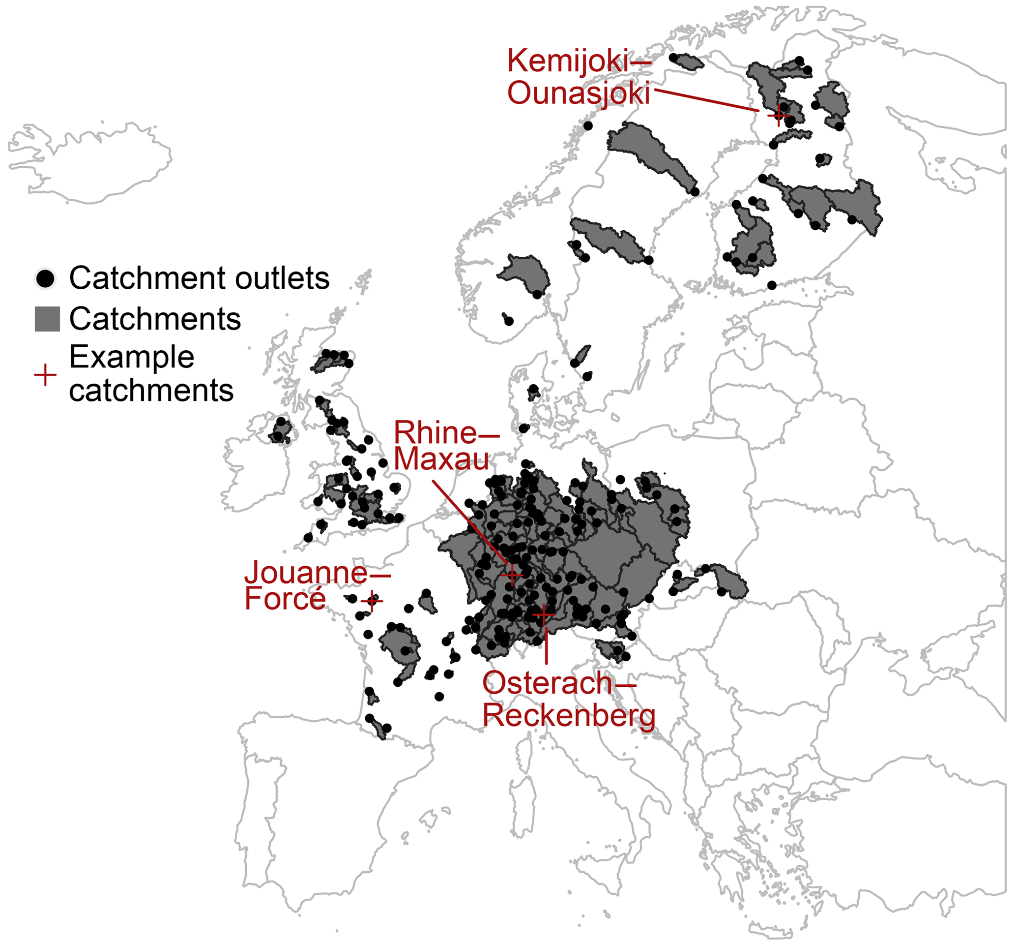
Figure 2 The 234 catchments in Central Europe selected for the analysis based on model performance and the availability of catchment boundaries and characteristics. The four example catchments, used for illustration purposes, are highlighted in red. (a) Kemijoki–Ounasjoki (strong summer flood regime). (b) Osterach–Reckenberg (summer flood regime). (c) Rhine–Maxau (winter flood regime). (d) Jouanne–Forcé (strong winter flood regime).

2.2 Data

EFAS provides deterministic and probabilistic medium-range streamflow forecasts and early warning information (Bartholmes et al., 2009; Smith et al., 2016). It relies on numerical weather predictions from the European Centre for Medium-Range Weather Forecasts (ECMWF), for which the initial conditions are derived using observed meteorological data, and the hydrological model LISFLOOD. LISFLOOD is a spatially distributed hydrological rainfall–runoff model based on Geographic Information Systems (GISs) developed by the Joint Research Centre (JRC) for operational flood forecasting at the pan-European scale (Thielen et al., 2009). EFAS v4.0 computes a water balance at a 6 h or daily time step for each grid cell (5 km × 5 km) using meteorological forcing data (precipitation, temperature, potential evapotranspiration, and evaporation rates). LISFLOOD represents a variety of processes (snowmelt, soil freezing, surface runoff, soil infiltration, preferential flow, soil moisture redistribution, drainage to the groundwater system, groundwater storage, and groundwater base flow) and routes the runoff produced for each grid cell through the river network using a kinematic wave approach. The model was calibrated using the modified Kling–Gupta efficiency metric (Gupta et al., 2009) for the period 1991–2017 for 1137 catchments for which discharge data were available (ECMWF, 2021).

In addition to streamflow forecasts, EFAS provides streamflow reforecasts generated by forcing LISFLOOD with medium- to sub-seasonal range meteorological reforecasts (Barnard et al., 2020), i.e. forecasts run for past periods (Hamill et al., 2006). The EFAS reforecasts cover the 20-year period from 1999–2018 and are initialized twice a week, on Mondays and Thursdays, with lead times of up to 46 d at a 6 h time step. They are driven with ensemble meteorological reforecasts from ECMWF's numerical weather prediction model. The meteorological ensemble consists of 10 perturbed ensemble runs which were derived using the same numerical weather prediction model but varying initial conditions.

2.3 Model and ensemble evaluation

We select the most suitable catchments for analysis out of 847 catchments in Central Europe which are part of the Global Runoff Data Centre database (GRDC; The Global Runoff Data Centre 56068 Koblenz Germany, 2019), have observations for the period 1991–2012, and whose catchment areas are similar to the upstream areas of the corresponding EFAS grid cells extracted using automatic coordinate matching (relative area difference < 20 %). Suitable catchments are identified by comparing observed streamflow with EFAS's historical simulations (generated with observed meteorological data and EFAS version 4.0). The evaluation focused on the period 1999–2012, as simulations are available from 1999 and observations until 2012. We computed different metrics which focus on high flows, including the Kling–Gupta efficiency metric (E_KG; Gupta et al., 2009) and the relative errors between simulated and observed 95 % (Q₉₅), 99 %, and 99.5 % quantiles. High-flow simulation performance varied among the 847 catchments, for which there may be several reasons, e.g. some catchments may be too small to guarantee reliable simulations given the 5×5 km model resolution. To ensure good performance in terms of high flows, we only retained catchments with good performance in terms of E_KG and Q₉₅. That is, we only choose stations with E_KG>0.6 and relative Q₉₅ errors < 10 %. The 234 catchments fulfilling these criteria are retained for further analysis (Fig. 2).

2.3.1 Data subsetting

The pooled frequency analysis relies on reforecasts of daily streamflow time series generated through EFAS v4.0. For our analysis, we use the 10 perturbed ensemble runs and 24 lead times, a subset of available lead times (l_t) chosen by picking every eighth lead time available (i.e. l_t=0, 48, 96, …, 1104 h). A subset was chosen as a trade-off between minimizing the computational feasibility and maximizing sample size.

2.3.2 Bias correction

Simulated streamflow time series can be biased because of uncertainties introduced through the modelling process. Substantial bias indicates low model fidelity because there is limited agreement between observed and modelled distributions (DelSole and Shukla, 2010). Potential uncertainty sources introducing bias include meteorological input uncertainty, due to the use of a numerical weather prediction system, and hydrological parameter and model uncertainties. Any such biases must be corrected in order to align the simulated streamflow distributions with observed distributions. To do so, we apply non-parametric quantile mapping, which has been found to be more flexible and suitable than parametric mapping approaches (Gudmundsson et al., 2012), to the daily simulated discharge series using the R package qmap (Gudmundsson, 2016). We estimate the empirical cumulative distribution function of the observed and simulated time series (reforecasts for different lead times and perturbations) for regularly spaced quantiles for the period 1999–2011 and for which both simulations and observations are available. Then, we apply quantile mapping to the simulated distributions of the whole period 1999–2018 for the different lead times and perturbations. We also tested another commonly applied bias correction procedure which maps the simulated distribution using the mean bias ratio on extracted extremes (as done in meteorological ensemble pooling studies, for example, by Kelder et al., 2020). However, we find that a correction by the mean bias ratio will still lead to biased flood estimates, especially for long return periods. A comparison of the cumulative distribution functions of observed and simulated flood events shows that both non-parametric quantile mapping and correction by the mean bias ratio lead to an alignment of the simulated with observed distributions and that quantile mapping produces more satisfactory results than correction by the mean bias ratio in most cases, especially for events with high non-exceedance probabilities (Fig. 3). Therefore, we use the series obtained by non-parametric quantile mapping for the pooled flood frequency analysis.

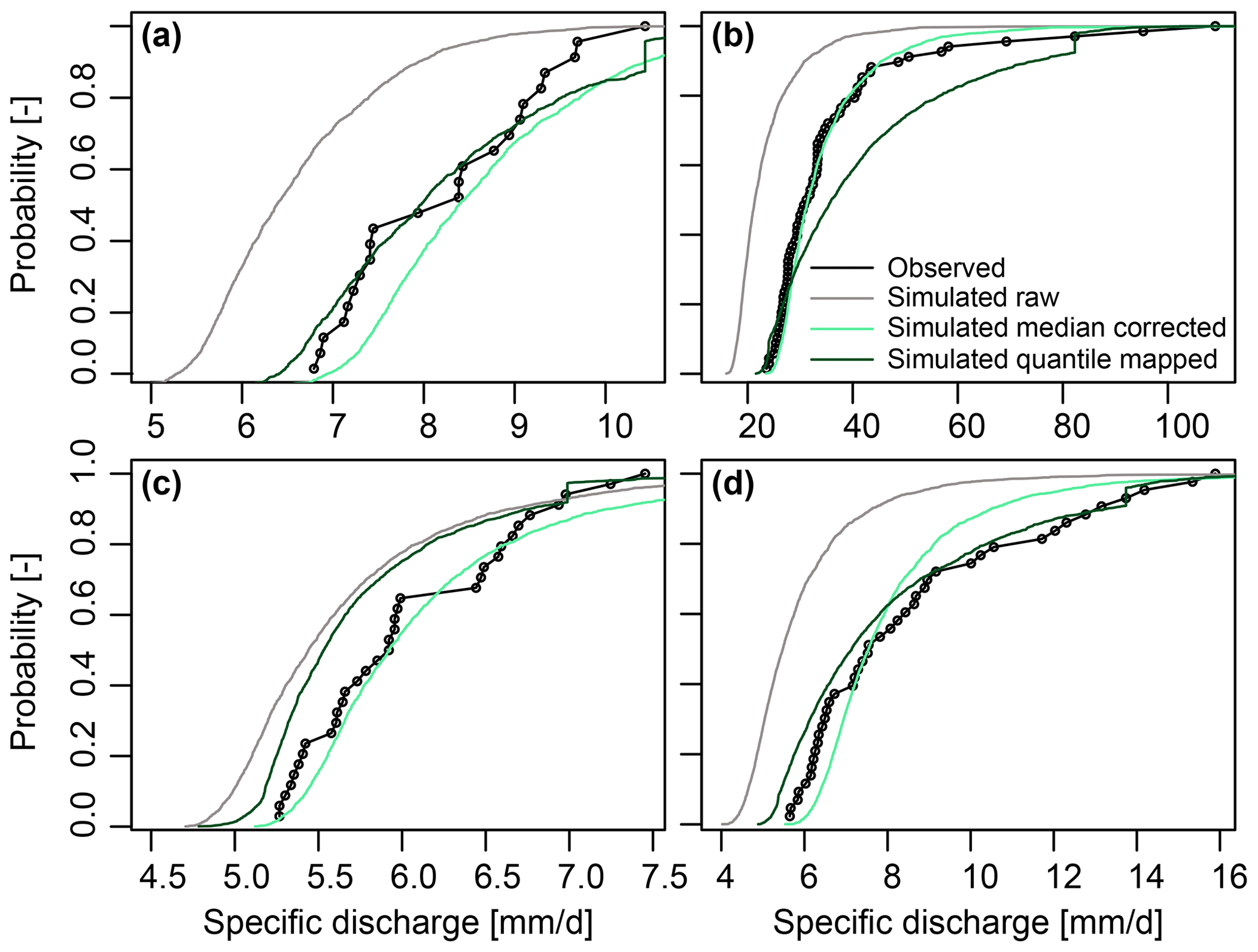
Figure 3 Comparison of observed and simulated cumulative distribution functions of peak-over-threshold flood events derived from observed streamflow time series, raw simulations without any bias correction, flood events corrected by the median ratio between observed and simulated flood distributions, and empirically quantile mapped simulations for the four example catchments. (a) Kemijoki–Ounasjoki. (b) Osterach–Reckenberg. (c) Rhine–Maxau. (d) Jouanne–Forcé.

2.3.3 Flood identification

After bias correction, we identify flood events in the time series simulated for different lead times and perturbed members (10 perturbed runs for each lead time). We use two flood extraction procedures, namely the annual maxima (AM) and peak-over-threshold (POT) approaches. Both approaches are applied to each of the simulated time series generated for different lead times (24) and perturbations (10), i.e. for 240 time series per catchment. The extracted AM event sets are used in the subsequent independence tests (see Sect. 2.3.4) because of their equal sample size across model runs (one event per year), which is not guaranteed for the POT event sets. However, POT events are used for the final frequency analysis (see Sect. 2.4) because POT samples include events that may be excluded when applying the AM approach. When applying the POT approach, the threshold is set to the 99th percentile, and independence between events is ensured by prescribing a minimum time window of 10 d between events (Diederen et al., 2019; Brunner et al., 2020a, b).

2.3.4 Stability and independence tests

Using the AM flood samples extracted from different simulation runs, we assess the suitability of the perturbed ensemble streamflow simulations for ensemble pooling by evaluating whether individual simulation runs can be considered independent and stable, i.e. that simulated distributions vary only slightly across lead times (Kelder et al., 2020).

First, we assess model stability, i.e. check whether the generated ensemble exhibits any changes in distribution with lead time. Ideally, a pooled ensemble should only exhibit weak changes in distribution with lead time. Such stability is assessed by comparing the distribution of AM events across different lead times (Fig. 4). To evaluate the model stability for a large number of catchments, we compute Spearman's correlation between simulated 95 % flood quantiles (20-year return period) and the corresponding lead times.

Second, we check whether individual model runs can be considered independent. Ensemble member independence is an important factor determining the increase in effective sample size achieved through ensemble pooling. If all x simulation runs are independent, pooling increases the effective sample size by x times. However, if the x simulation runs show a higher degree of dependence, pooling increases the sample size by y<x times. We calculate Spearman's rank correlation using the pairs of AM time series (following Kelder et al., 2020; Fig. 5). Note that such a correlation can directly only be computed for AM and not for the peak-over-threshold (POT) series because the POT series may differ across ensemble members in terms of the number of events chosen for analysis. Therefore, it can be assumed that the POT events used in our subsequent analyses are more independent than AM events. To illustrate the difference between dependence in AM and POT samples, we indirectly compute Spearman's correlation for pairs of POT time series by using events where at least one of the time series exceeds a threshold. For this correlation analysis, we replace non-exceedances in the paired time series by 0 (which is not ideal because this might artificially introduce some sort of dependence).

2.4 Frequency analysis

For the frequency analysis, we use the POT instead of AM flood samples to ensure the inclusion of relevant events and to reduce the dependence between ensemble members (i.e. runs for different lead times and for different perturbations).

2.4.1 Local frequency analysis

For the local (catchment-specific) frequency analysis, we pool all POT events from the perturbed members of the lead times that can be considered independent, i.e. lead times ≥ 528 h or 22 d (see Sect. 3.1). Such pooling increases the sample size available for frequency analysis from $\mathrm{1}\times \sim \mathrm{20}$ events (roughly one event chosen per year on average) to 13 lead times × 10 members × 20 events = 2600 events.

We fit a theoretical generalized Pareto distribution (GPD; Coles, 2001) to the observed and pooled POT samples using the maximum likelihood estimation. We use the fitted distributions to derive best estimate observed and simulated flood frequency curves using probabilities corresponding to return periods between 1 and 200 years. In addition, we derive 90 % confidence intervals for the observed and simulated frequency curves using bootstrapping, i.e. we draw n=1000 random samples from the observed and simulated samples, respectively, to derive 1000 theoretical flood frequency curves. We then use these resampled frequency curves to compute 90 % confidence intervals for the estimated flood frequency curves. We compare simulated to observed flood quantiles corresponding to return periods of T=5, 10, 20, 50, 100, and 200 years by computing relative differences between simulated and observed quantiles. Furthermore, we compare the uncertainty of these estimates by computing the relative difference in the range between the 95 % and 5 % quantile of the 1000 resampled estimates for each return period.

As a reference for these theoretical estimates, we provide empirical return period estimates of the observed flood events derived using the Weibull plotting position $T_{\mathrm{wb}}=m/(N+\mathrm{1})$, where N is the total number of events, and m is the rank of an event within the sample. To also represent the uncertainty of these empirical estimates, we perform another bootstrapping experiment, which derives the plotting positions for different samples by removing 1 year at a time. Next, we map the flood quantiles estimated for return periods of T=10, 20, 50, 100, and 200 years for the 234 catchments using the GPD distributions fitted to the pooled POT samples.

To identify physiographical and hydrometeorological characteristics important for explaining flood quantiles at different return periods, we use linear modelling. We fit different linear regression models of different sizes, i.e. with different numbers of explanatory variables, using exhaustive search (James et al., 2013) to predict flood quantiles with a specific return period, e.g. 10 years. For the exhaustive search (i.e. trying all variable combinations), we use a set of potential explanatory variables frequently used to explain flood characteristics, including altitude, catchment area, number of dams in catchment, mean slope, population count, mean temperature, mean precipitation, mean evapotranspiration, mean snow water equivalent (SWE), mean snowmelt, and mean soil moisture. We computed the mean areal hydrometeorological characteristics, including precipitation, temperature, evapotranspiration, SWE, snowmelt, and soil moisture (average over four layers) using the gridded ERA5-Land data set (Muñoz Sabater, 2019). Among the fitted models with different numbers of predictors, we identify the model with the smallest Bayesian information criterion (BIC) value for each return period and look at the explanatory variables retained in these models. The sign and magnitude of the retained regression coefficients are used to describe the importance of each predictor in explaining flood quantiles for different return periods.

2.4.2 Regional frequency analysis

After performing the local frequency analysis, we look at probabilities of regional flooding. That is, we estimate the return periods of events that affect a certain percentage of catchments within a larger region, i.e. river basin. We focus on the major river basins in Europe (HydroSHEDS; Lehner and Grill, 2013) and ask what is the probability that 30 %, 50 %, and 70 % of the catchments in each of these river basins are jointly affected by flooding. To compute such regional flooding probabilities, we follow the regional hazard estimation procedure proposed by Brunner et al. (2020b). For each large river basin, we (1) determine the available catchments located within the given region and focus on river basins with at least five catchments (out of the 234), (2) identify the number of flood events during which p(%) of the catchments are jointly flooded using a binary flood event matrix, which indicates for each catchment whether it was affected by specific flood events identified across all catchments, lead times, and perturbed members, and (3) compute the probability of regional flooding using the Weibull plotting position given by the following:

$$\begin{array}{}\text{(1)}& p\left(\mathit{\%}\right)=\mathrm{100}(x/(n+\mathrm{1}\left)\right),\end{array}$$

where n is the total number of events affecting at least one of the stations in the region, and x is the number of events where y% of the stations were affected by flooding.

3 Results

3.1 Ensemble evaluation

After identifying catchments with satisfactory model performance in terms of the EFAS historical runs, we assess the suitability of the streamflow ensemble generated using the perturbed numerical weather predictions and different lead times for ensemble pooling. This assessment focuses on AM instead of POT flood samples because POT event identification can lead to the selection of an unequal number of events across lead times, which makes it impossible to compute correlations. We first consider the stability (i.e. lack of drift across lead times) of annual maxima flood events simulated for 24 lead times ranging from 0 to 46 d for one example catchment (Fig. 4). Within each year, flood magnitudes do not differ systematically across lead times (Fig. 4a), and cumulative flood distributions seem to be stable across lead times (Fig. 4b).

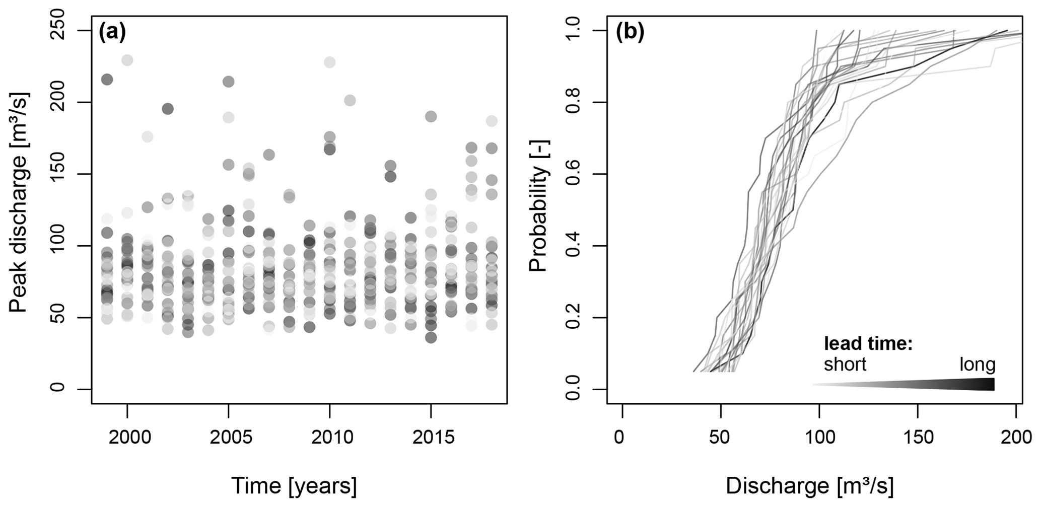
Figure 4 Stability across lead times from 0 to 46 d for one example catchment. (a) AM flood events extracted from streamflow time series simulated for 24 lead times (one dot per lead time). (b) Cumulative distribution functions of AM flood samples per lead time (one line per lead time). The darker the colour, the longer the lead time.

We take a closer look at model stability for all catchments by assessing the dependence of the empirical 95 % flood quantile on lead time, using Spearman's correlation coefficient. The median correlation between the lead time and the simulated 95 % quantile across all catchments is 0.02, and the lower and upper quartiles are −0.32 and 0.35, respectively. That is, in most catchments, simulated flood quantiles are only weakly dependent on the lead time, which suggests overall model stability. Some individual catchments may exhibit greater (positive or negative) forecast drift than others, and so researchers may wish to assess the model stability more closely when working on individual case studies.

We now take a look at AM (in)dependence across perturbed ensemble members by computing Spearman's rank correlation between pairs of AM series derived for the 10 perturbed ensemble members at each lead time. AM (in)dependence across perturbed ensemble members seems to depend both on the catchment and on lead time (Fig. 5). Dependence is relatively high for short lead times and decreases with longer lead times. The strength of the dependence at t=0, and the rate of decrease with increasing lead time, depends on the catchment as illustrated by the different dependence decay behaviour of the four example catchments. While some catchments (e.g. Fig. 5b and d) show correlation values close to 0 for sufficiently long lead times, other catchments (e.g. Fig. 5a) show relatively high correlations of 0.5 even at lead times exceeding 1 month. That is, individual AM series for different ensemble members may not necessarily be fully independent in a hydrological context. This finding contrasts with independence tests performed for other types of extremes such as extreme precipitation (Kelder et al., 2020) or wind (Breivik et al., 2014), which found that simulated precipitation and wind extremes can be considered independent after certain lead times. The residual dependence in the case of hydrological simulations is likely caused by the long memory of hydrological systems, which is related to storage processes in the soil or the cryosphere and the persistence of the effects of initial conditions on the model forecasts. Such residual dependence would be expected to be independent of the choice of hydrological model used to translate the independent precipitation series to streamflow.

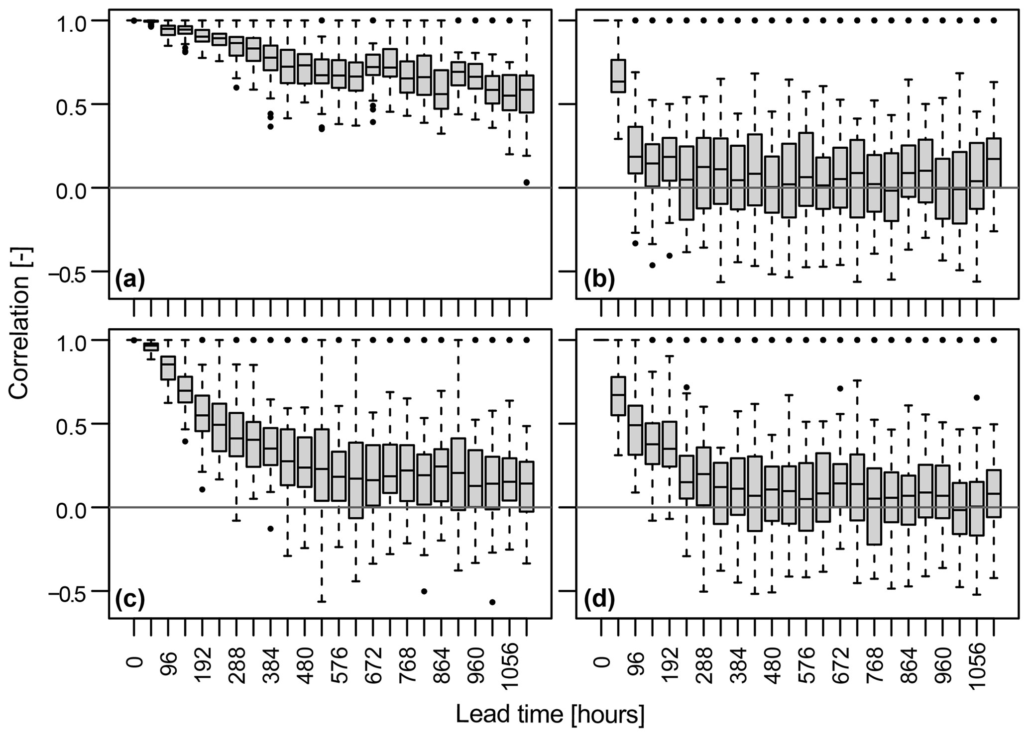
Figure 5 Member (in)dependence (Spearman's correlation) per lead time – 0 to 110 h (46 d) – across the 10 perturbed ensemble members for four example stations with different flood seasonality ratios (strong summer vs. strong winter flood regime; clockwise from upper left to lower right). (a) Kemijoki–Ounasjoki (strong summer flood regime). (b) Osterach–Reckenberg (summer flood regime). (c) Rhine–Maxau (winter flood regime). (d) Jouanne–Forcé (strong winter flood regime; Fig. 2).

We seek to better understand which types of catchments show high/low ensemble member dependence across lead times. Therefore, we compute the median Spearman's rank correlation across the 10 ensemble members and 24 lead times for each of the 234 catchments and try to relate this median correlation to a catchment's flood seasonality ratio. The flood seasonality ratio R_F is computed as $R_{\mathrm{F}}=Q_{\mathrm{95}\mathrm{s}}/Q_{\mathrm{95}\mathrm{w}}$, where Q_95s represents Q₉₅ in summer (April–September), and Q_95w represents Q₉₅ in winter (October–March). R_F>1 and <1 represent catchments with more severe summer than winter floods and more severe winter than summer floods, respectively. We also considered other metrics to explain median lead time correlation, such as the baseflow index (Ladson et al., 2013) or catchment area, but did not find any meaningful relationships. Median lead time dependence shows clear spatial patterns with higher dependencies in the Alps and Scandinavia than in the rest of Europe (Fig. 6a). These regions with higher median dependencies are characterized by a summer flood regime, as they are partly influenced by snowmelt contributions (Berghuijs et al., 2019). The median lead time correlation seems to generally increase with higher seasonality ratios (Fig. 6b), i.e. the more summer-/snow-dominated a flood regime is, the higher the AM dependence. However, some of the winter-/precipitation-dominated regimes can also have high dependence values.

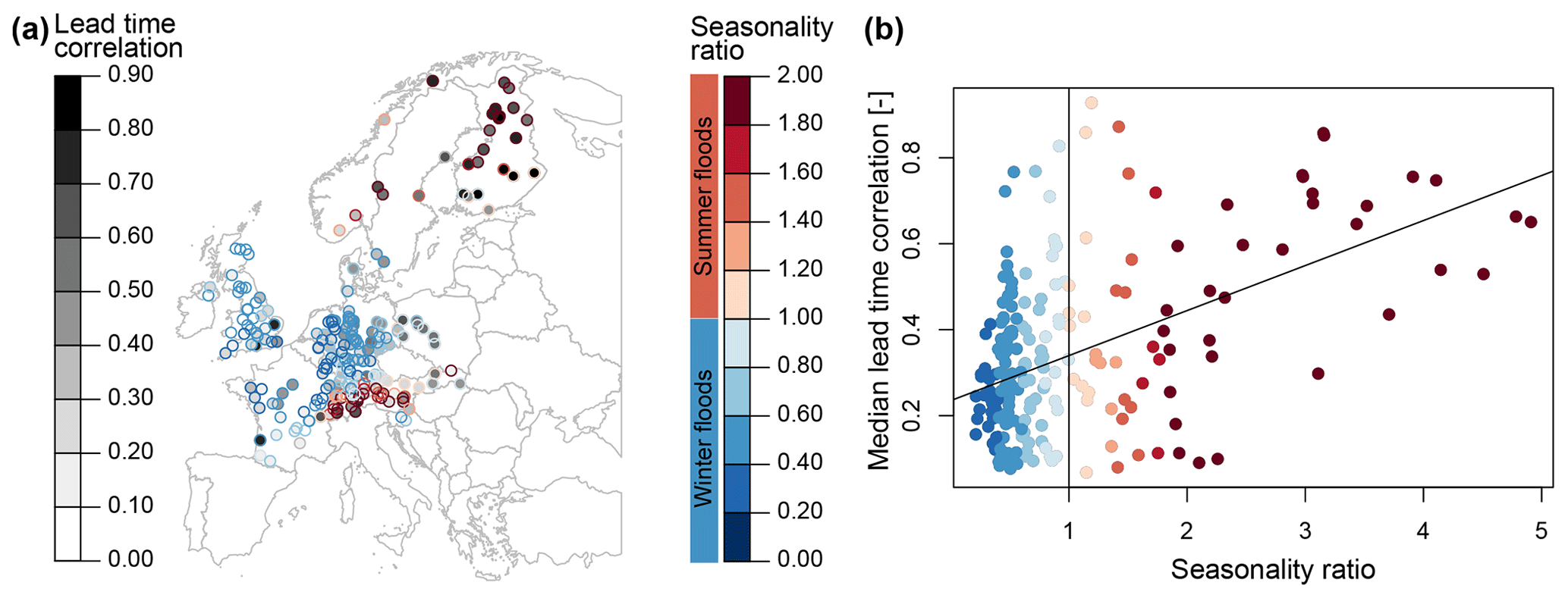
Figure 6 Median annual maxima dependence across all lead times and ensemble members per catchment. (a) Spatial variation in median correlation (grey outlines) and seasonality ratio, where red colours indicate higher floods (Q₉₅) in summer than winter and blue colours indicate higher floods in winter than summer. (b) The relationship between the median correlation and seasonality ratio, where the vertical black line indicates the transition from winter- to summer-dominated flood regimes, and the trend line was derived using linear regression.

Figure 7 Median Spearman's correlation across ensemble members and catchments per lead time (0 to 1104 h) for (a) annual maxima and (b) peak-over-threshold events. The median correlation per lead time is indicated by the horizontal grey line, and the break point in this median series derived by the Pettitt test at the vertical red line. No red line is shown in panel (b), as the break point was determined using the AM series shown in panel (a).

The high dependence at low lead times suggests that simulations at lower lead times should be removed before pooling flood events for frequency analysis. In order to determine the lead times to be excluded, we compute median AM dependence across ensemble members and catchments for each lead time and perform a Pettitt change point test (Ryberg et al., 2020) on the resulting median time series (Fig. 7a). The change point analysis suggests that dependence values stabilize, on average, at around 528 h, i.e. 22 d. As an alternative to using a single threshold for all catchments, one could use a variable threshold, which is lower for catchments with lower dependence values and higher for catchments with higher dependence values. We decided to work with one single threshold for simplicity. The implementation of a 22 d independence threshold compares well with the independence thresholds identified and used in previous studies applying reforecast pooling (10 d in Breivik et al., 2014; 30 d in Kelder et al., 2020). Our flood frequency analysis therefore pools flood events derived from the streamflow time series of the 10 perturbed members for each lead time > 22 d. Such pooling allows us to substantially increase the sample size (i.e. 130 times, that is 13 lead times and 10 perturbed runs). To further reduce dependence, our analysis relies on peak-over-threshold instead of annual maxima events (Fig. 7b), which substantially reduces dependence at all lead times if we compute Spearman's rank correlation for exceedance time series, where non-exceedances are replaced by 0 (Breivik et al., 2013).

3.2 Flood frequency analysis

Flood estimates derived by theoretical distributions fitted to pooled peak-over-threshold (POT) flood events from 10 ensemble members and 13 lead times are more robust, i.e. have smaller uncertainty, than flood estimates derived from distributions fitted to a small sample of observed POT events, as illustrated in Fig. 8 for four example catchments (Fig. 2). Observation- and simulation-based estimates do not just differ in terms of uncertainty but also in terms of the magnitudes of the best estimates.

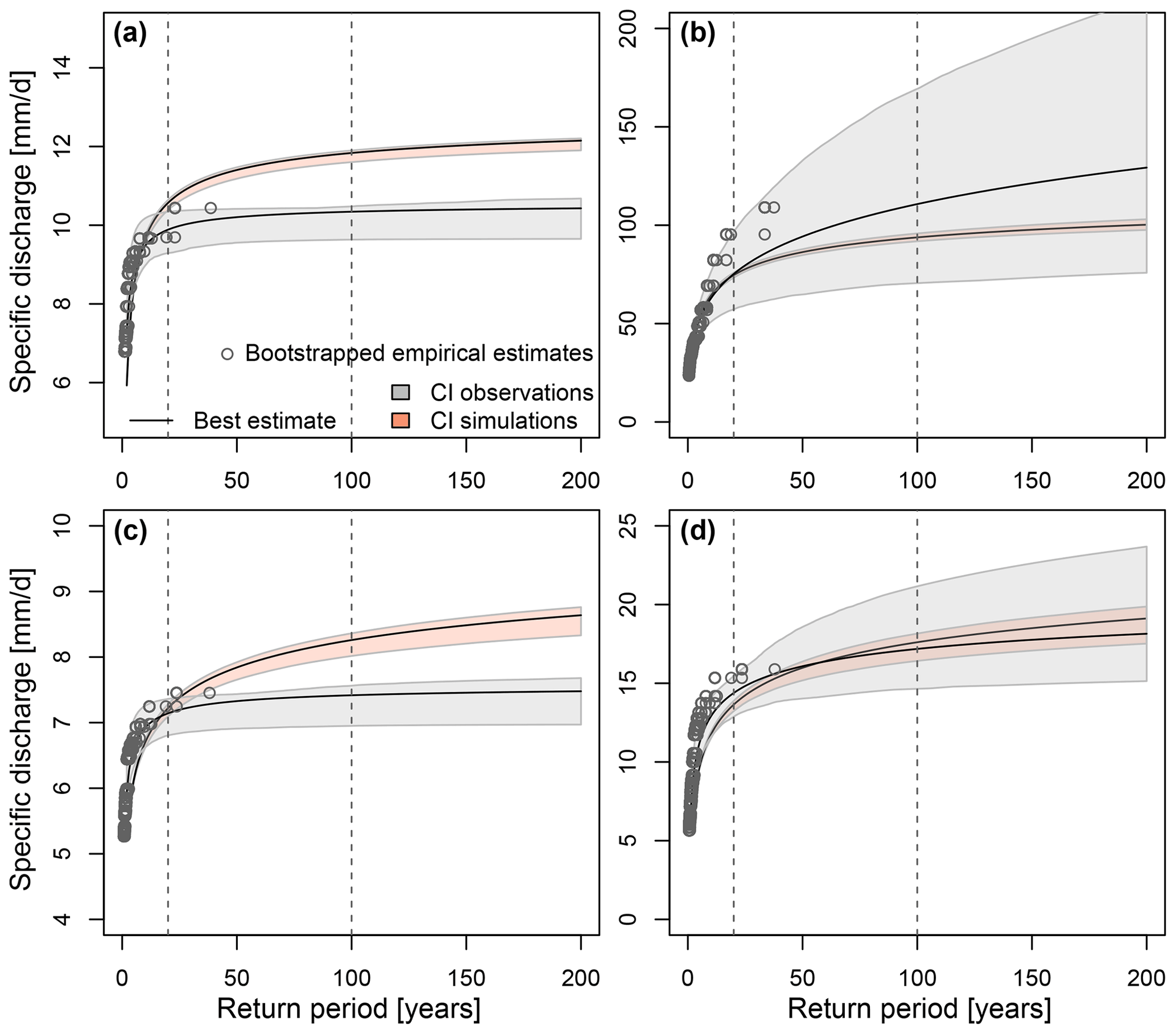
Figure 8 Observed vs. simulated flood frequency curves, including uncertainty bounds for four example catchments with different seasonality ratios. (a) Kemijoki–Ounasjoki. (b) Osterach–Reckenberg. (c) Rhine–Maxau. (d) Jouanne–Forcé. The observed and simulated best estimate frequency curves are indicated by black lines, the corresponding 90 % confidence intervals by shaded polygons, and bootstrapped empirical return period estimates by grey dots. Confidence intervals are derived using bootstrapping.

The differences between observation- and simulation-based best estimates and uncertainty ranges vary by return period and by catchment (Fig. 9). Relative differences between observation- and simulation-derived best estimates are mostly positive, i.e. observed quantiles tend to be larger than simulated quantiles (Fig. 9a). These relative differences increase with the return period length. Similarly, observation-derived uncertainty ranges are wider than simulation-derived uncertainty ranges, and these differences also increase with the return period length (Fig. 9b). Both the relative differences in best estimates and uncertainty bounds depend on catchment area and elevation to some degree (Fig. 9c and d). Low-elevation and large catchments generally show lower relative differences in the best estimates and uncertainty than high-elevation and small catchments. As the effect of area on relative differences is stronger than the effect of elevation, there are no clear spatial patterns in the relative differences between observed and simulated best estimates and uncertainty bounds. Please also note that the relative differences between simulated and observed best estimates and uncertainty bounds are uncorrelated with model performance, which means that increasing the cutoff threshold for EFAS model performance (level of E_KG) does not necessarily lead to an increase in the similarity between observed and simulated flood estimates.

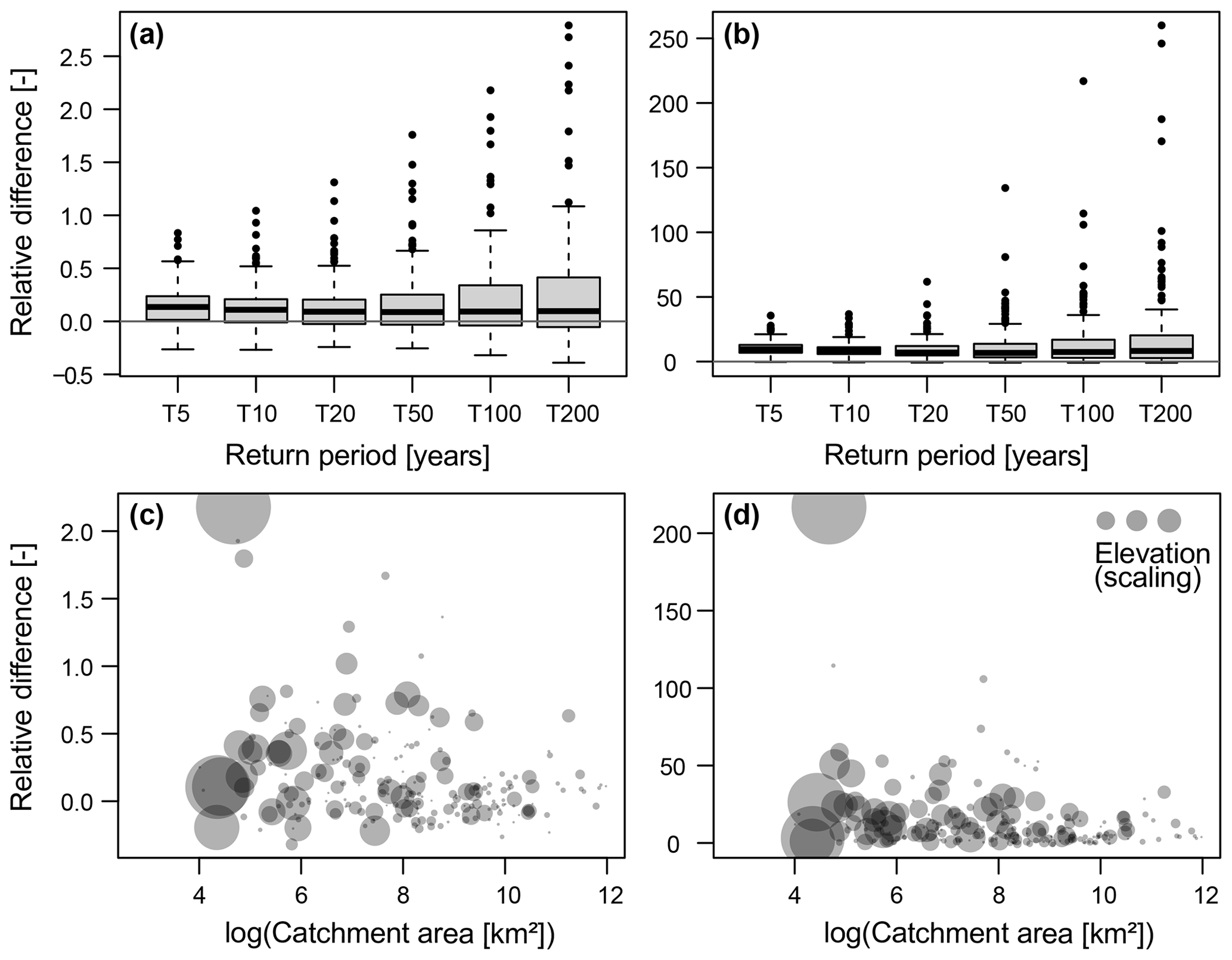
Figure 9 Relative difference between the observed and simulated ((obs-sim)/sim) (a) best estimates and (b) the range of uncertainty bounds (Q₉₅−Q₀₅) for different return periods (5, 10, 20, 50, 100, and 200 years) across catchments (one point in the box plot corresponds to one catchment). Relative difference between the observed and simulated ((obs-sim)/sim) (c) best estimates and (d) the range of uncertainty bounds (Q₉₅−Q₀₅) for the 100-year return period in relation to catchment area and elevation. The larger the dot, the higher elevation of a catchment.

We now use the best estimates derived by ensemble pooling to map spatial patterns of flood quantiles over Central Europe for different return periods (Fig. 10). Flood quantiles are highest in the Alps and Great Britain and lowest in northern Germany and Scandinavia, independent of the return period. These spatial patterns corroborate previous findings that the Alps and Great Britain are regions with a comparably high number of flood events per year (Mangini et al., 2018), and that observation-based 100-year specific discharge is highest in the Alps, Great Britain, and Norway and lowest along the Atlantic coast (Blöschl et al., 2019). Additionally, we find that the local flood quantiles are positively related to mean slope and mean precipitation of a catchment and negatively related to the number of dams, temperature, and mean snowmelt of a catchment (Fig. 11). In other words, catchments with steep slopes, colder climates, and higher mean precipitation tend to have higher flood quantiles, while catchments with a greater number of dams and higher snowmelt contributions tend to have smaller flood quantiles.

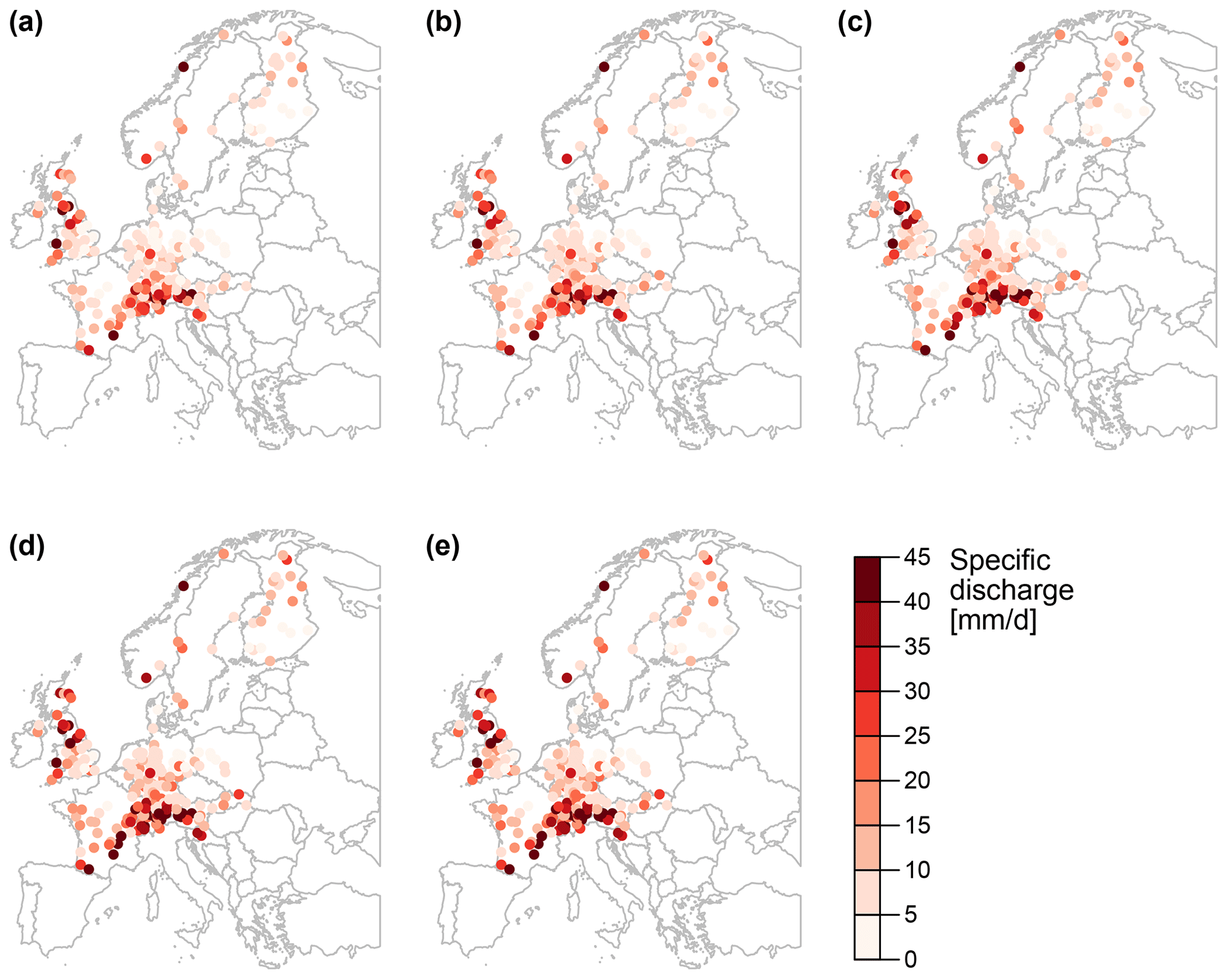
Figure 10 Theoretical flood quantiles corresponding to return periods of (a) 10, (b) 20, (c) 50, (d) 100, and (e) 200 years derived from pooling POT events extracted from time series simulated for 10 ensemble members and 13 lead times (≥528 h; sample size = 2600; 13 lead times × 10 members × 20 years).

Figure 11 Predictor importance for flood quantiles. Regression coefficients for significant explanatory variables retained when choosing the linear model with the lowest BIC (α=0.05). Green and red colours indicate positive and negative relationships between flood estimates and catchment characteristics, respectively. Grey colours indicate non-included (i.e. non-significant) explanatory variables.

Ensemble pooling can also be used to derive regional flood estimates, i.e. to compute the probability that a certain percentage of catchments within a region, i.e. large river basin, are jointly flooded (Fig. 12). Regional floods with a 30 % coverage, i.e. floods affecting at least 30 % of the catchments within a region, occur relatively frequently (return periods < 10 years) both in Central Europe and Scandinavia (Fig. 12a). In contrast, regional events with a 50 % coverage are more likely in Central Europe (lighter colours) than in Scandinavia (darker colours). Very widespread events with 70 % spatial coverage become very rare (return periods > 90 years) in most parts of Europe, except in the Weser, Elbe, and Oder river basins.

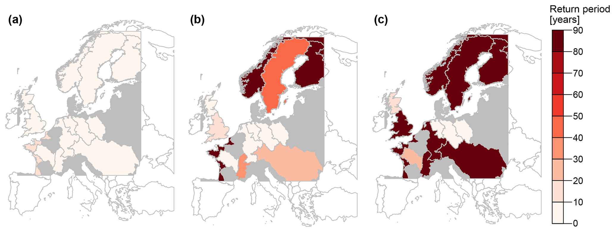
Figure 12 Probabilities of regional flooding for European river basins with more than five catchments, with (a) 30 % affected, (b) 50 % affected, and (c) 70 % affected. Regions with less than five catchments where regional flood probabilities could not be determined are highlighted in grey, and regions not covered by our data set are displayed in white.

4 Discussion

Pooling flood events derived from a streamflow reforecast ensemble substantially increases the sample size available for flood frequency analysis. In doing so, it enables the study of very rare extremes absent in relatively short observed time series. Increasing the sample size also facilitates the study of spatial patterns in the distribution of flood estimates corresponding to long return periods (e.g. 200 years; Fig. 10e) and notably reduces uncertainty in most cases (Fig. 9b), independent of the original EFAS model performance. Furthermore, it enables the study of rare spatial extremes, i.e. events that may affect multiple catchments at once (Fig. 12). Therefore, streamflow reforecast ensemble pooling represents a suitable alternative to stochastic or climate model large ensemble approaches for studying the frequency and magnitude of rare extreme events. Similar to large ensemble approaches, but in contrast to stochastic approaches, reforecast-based simulation approaches rely on physical representations of the hydrological cycle. Such a physical representation may be especially valuable if relationships between different variables are of interest and if one wishes to study the physical drivers of flood events. In contrast, stochastic models have the advantage of being relatively straightforward to implement and are potentially less computationally intense.

The utility of reforecast pooling rests on the performance of the underlying hydrological simulations. The use of reforecast simulations instead of observations comes at the cost of potentially introducing uncertainty through simulated meteorological input or the hydrological model itself (structure and parameters; Clark et al., 2016). These uncertainties may result in biased simulations, which may either under- or overestimate the whole or specific parts of the streamflow distribution. Such bias can be partly reduced by using bias correction techniques such as quantile mapping (Fig. 3). Yet, the plausibility of unprecedented extremes relies on the realism of hydrological simulation in the model system, i.e. a reliable representation of hydrological processes and their drivers. Further improvement in the model representation of high flows may be needed to reduce bias and improve process representation (Mizukami et al., 2019; Brunner et al., 2021a).

An additional limitation is the spatial applicability of the approach. As hydrological model simulations must be bias corrected, the use of ensemble pooling is currently limited to catchments for which streamflow observations are available. This requirement limits the application of the pooling approach to gauged catchments. In theory, using simulations instead of observations would enable the extension of the spatial coverage to ungauged locations. However, such an extension would only be possible if no bias correction was required or if bias correction could be regionalized and applied to all catchments.

Sample size is only effectively increased compared to observations if the simulated flood samples for different ensemble members can be considered independent (Kelder et al., 2020). However, such independence is more difficult to achieve in hydrological than meteorological systems, as hydrological systems exhibit substantial memory effects, for example, through snow or soil moisture storage (Berghuijs et al., 2019; Brunner et al., 2020a). These memory effects introduce varying degrees of dependence to ensembles of simulated annual maxima time series (Fig. 5). The dependence is highest in catchments with high seasonality and where floods predominantly occur in summer under the potential influence of snowmelt (Fig. 6). The dependence does not depend strongly on variables which typically affect streamflow persistence, such as catchment area or baseflow index. Still, any such dependence can be notably decreased if annual maxima events are replaced by peak-over-threshold events. Using POT events has the advantage that, besides event magnitudes and timing, the number of events may also vary. This approach means that a one-to-one relationship between events extracted from two different ensemble members can no longer be established.

The flood ensemble pooling approach described herein is not limited to the EFAS reforecasts over Europe but could also be applied to other streamflow reforecast modelling systems, such as the Global Flood Awareness System (GloFAS; Alfieri et al., 2013) or the Global Flood Forecasting Information System (GLOFFIS; Emerton et al., 2016). Moreover, the pooling approach may be beneficial to other types of hydrological extremes beyond flood frequency analysis, such as droughts. Such an extension would require model evaluation targeted at the variables of interest. Hydrological extremes extracted from streamflow reforecasts may also be used in combination with climatic extremes extracted from meteorological reforecasts to study the frequency of compound events (such as joint pluvial and fluvial flooding) or the drivers of various extremes. In any case, the use of simulated extremes pooling requires careful model evaluation and is likely to require some form of bias correction to ensure the fidelity of extremes.

5 Conclusions

Pooling of publicly accessible reforecast flood events such as those generated through the European Flood Awareness System (EFAS) can be a useful tool to improve the robustness of flood estimates, particularly for rare events with long return periods. However, as with other extremes (Kelder et al., 2020), such pooling is only effective if simulated floods show little bias and model drift across lead times and if the floods extracted from different ensemble members are sufficiently independent to increase the effective sample size available for frequency analysis. Bias can be removed using bias correction techniques such as quantile mapping. The degree of dependence is subject to the catchment (with summer-flood-dominated catchments showing higher dependencies than winter-flood-dominated catchments), lead time (with decreasing dependence at longer lead times), and event type (with peak-over-threshold events showing lower dependence than annual maxima events). The higher dependence of summer-flood-dominated catchments than winter-flood-dominated catchments suggests that catchment memory through snow storage effects is an important determinant of dependence, and that catchments with a more predictable seasonality may have greater member dependence. We recommend pooling peak-over-threshold events from ensemble runs generated for lead times > 22 d because floods are less dependent, on average, beyond such a lead time and because dependence is lower for POT than AM events.

Our application of the pooling approach over 234 European catchments shows that local floods are most extreme in the Alps and Great Britain and least extreme in Scandinavia and Central Europe. It also indicates that regional extreme flood events, in which a large fraction of catchments flood simultaneously, are more likely in Central Europe than in Scandinavia. We conclude that pooled reforecast ensembles are beneficial in studying the probability of extreme and spatially extensive events in the case of accurate model representation of hydrologic extremes, as they help provide flood estimates with considerably reduced uncertainty compared to observation-derived flood estimates.