Technical note: High Nash–Sutcliffe Efficiencies conceal poor simulations of interannual variance in seasonal regimes

In highly seasonal regimes hydrologic models generally achieve high scores on common performance metrics such as the Nash–Sutcliffe Efficiency (NSE) and the Kling–Gupta Efficiency (KGE). However, variance in streamflow time series is composed of seasonal, interannual, and irregular variance, and the NSE and KGE do not differentiate between these components. Differences in performance on these three components have not been evaluated across a broad spectrum of hydrologic models and regions. We analyse open-access simulations from 18 regional and global hydrologic models. We find that these models consistently achieve the highest NSE and KGE in highly seasonal catchments where they are worse at simulating interannual variability, compared to less seasonal catchments. Simulated year-to-year changes in ecologically relevant hydrologic signatures are less accurate in highly seasonal catchments, and the NSE of the interannual variance component is usually lower. This suggests that these hydrologic models may struggle to predict long-term responses to climate change, especially in highly seasonal tropical, alpine, and polar regions, which are some of the most vulnerable to climate change. We encourage hydrologic modellers to explicitly evaluate skill at simulating interannual variability, rather than relying only on aggregate measures such as the NSE and KGE.

1 Introduction

Interannual variability and change in streamflow threatens social and ecological systems, as aquatic species are adapted to the natural streamflow regime (McMillan, 2021; Poff et al., 1997; Poff and Zimmerman, 2010), and unpredictable water availability hinders effective water resource management (Hall et al., 2014). The earth's changing climate is exposing non-stationarities in streamflow regimes (Milly et al., 2008), which have been detected in hydrologic signatures such as mean flows and the frequency, duration, and magnitude of hydrologic extremes (Gudmundsson et al., 2021; Ruzzante and Gleeson, 2025; Slater et al., 2021; Taye and Dyer, 2024; Xiong and Yang, 2024), and changes in the timing of streamflow (Berghuijs et al., 2025; Stewart et al., 2005; Wasko et al., 2020). However, there is a disconnect between how hydrologic change is assessed (using hydrologic signatures) and how hydrologic models are typically calibrated/trained and evaluated (using aggregate performance metrics), which may lead to inaccurate predictions of hydrologic change.

Streamflow time series can be conceptualized as the sum of seasonal, interannual, and irregular variance components, with very different driving mechanisms for each component. Stochasticity in individual weather events drives irregular variance (sometimes called remainder, noise, or high-frequency variance) while more regular seasonal cycles of temperature and precipitation drive seasonal fluctuations of the hydrograph (Dralle et al., 2017). Interannual variance, on the other hand, can be driven by climate oscillations, climate change, and other non-stationarities such as vegetation responses to climate change.

Hydrologic models, in contrast, are typically assessed on their aggregated ability to reproduce a historical timeseries of observations (Eker et al., 2018). In a climate change context, we desire hydrologic models that accurately predict historical interannual variability and change (Milly et al., 2008; Montanari et al., 2013; Wagener et al., 2010) and use performance on historical data as a proxy for their performance in future cases. However, hydrologists rarely consider interannual variability separately and the most popular performance metrics (the Nash–Sutcliffe and Kling–Gupta Efficiencies, NSE and KGE) evaluate all three variance components in an aggregated manner (i.e., as a single number; Gupta et al., 2009; Kling et al., 2012; Nash and Sutcliffe, 1970).

However, good performance on one variability component does not guarantee good performance on the others because the driving mechanisms of interannual, seasonal, and irregular variability are different. We hypothesize that in catchments where one component historically dominates variability, model calibration/training will emphasize simulation accuracy of the dominant component, whereas the other components will be more poorly simulated. Specifically, we aim to test whether interannual variance is poorly modelled in catchments with a strong seasonal cycle, because locations where strong seasonal cycles are common (e.g., tropical basins, snow-dominated mountain ranges, and high-latitude locations) are also extremely vulnerable to climate change.

The concept of a “strong” seasonal cycle has been discussed at some length and quantified in the context of climatological benchmark models, which are typically defined as the interannual mean flow for each calendar day. Garrick et al. (1978) were among the first to propose that a model should outperform the climatological benchmark, and subsequent authors found that the climatological benchmark NSE values, here denoted as NSE_cb, can be very high (sometimes greater than 0.8) in high-mountain catchments (Martinec and Rango, 1989; Schaefli and Gupta, 2007). Knoben (2024) similarly found that benchmark KGEs are high in snow-dominated regions.

We aim to answer 3 questions:

• 1.

  Where are the interannual, seasonal, and irregular components of streamflow variance dominant?

• 2.

  Where is the climatological benchmark NSE high?

• 3.

  What does this mean for our ability to simulate long-term change in a nonstationary world?

In Sect. 4.1 we address Question 1. We use time series decomposition on global stream gauge data from 18 open-access datasets and calculate the variance fraction for each component. We then address Question 2 in Sect. 4.2 and calculate the climatological benchmark NSE for 20 338 stream gauges. In Sect. 2.1 we also explain that the climatological benchmark NSE is equivalent to the seasonal variance fraction.

Regarding Question 3, we expect that hydrologic models will be worse at representing interannual variability (and long-term change) in highly seasonal catchments because in these catchments “high” NSE scores can be achieved without accurately representing the hydrologic processes that lead to interannual variability (for example, in the climatological benchmark model). In Sect. 4.3 we test this hypothesis with open-access simulations from 18 hydrologic models.

2 Methods

2.1 Time Series Decomposition

To address Question 1, we applied time series decomposition techniques to streamflow data from 17 245 gauges. From our compilation of 28 406 daily discharge time series (see Sect. 3.1), we selected the 17 245 with at least 10 years of data without missing days. We decomposed each time series into seasonal, interannual, and irregular components. First, we deseasonalized the data: that is, we calculated the seasonal component as the mean of each calendar day and subtracted this from the observed time series to extract the deseasonalized anomalies. We calculated the Fast Fourier Transform of the anomalies and separated the Fourier frequencies into interannual (frequencies smaller than 2 year⁻¹) and irregular components (frequencies greater than or equal to 2 year⁻¹). We chose a cutoff frequency of 2 year⁻¹, or a period of 6 months, in order to classify variations in seasonality (e.g., a wetter than normal summer) as interannual variance. Additional details and a flowchart are provided in Sect. S3 in the Supplement.

This decomposition is orthogonal so the sum of the variances of the components $({\mathit{\sigma }}_{\text{interannual}}^{\mathrm{2}}+{\mathit{\sigma }}_{\text{seasonal}}^{\mathrm{2}}+{\mathit{\sigma }}_{\text{irregular}}^{\mathrm{2}}$) is equal to the variance of the observed streamflow time series $({\mathit{\sigma }}_{\mathrm{o}}^{\mathrm{2}}$). For each catchment we calculated the variance fraction associated with each component, (e.g., ${\mathit{\sigma }}_{\text{seasonal}}^{\mathrm{2}}/{\mathit{\sigma }}_{\mathrm{o}}^{\mathrm{2}}$). Because the decomposition is orthogonal the three variance fractions sum to 1. Another result of this orthogonality is that the variance fraction is identical to the NSE for each component. For example, the seasonal variance fraction is equivalent to the climatological benchmark NSE_cb:

$$\begin{array}{}\text{(1)}& {\mathrm{NSE}}_{\mathrm{cb}}=\mathrm{1}-{\displaystyle \frac{{\mathit{\sigma }}_{\mathit{ϵ}}^{\mathrm{2}}}{{\mathit{\sigma }}_{\mathrm{o}}^{\mathrm{2}}}}=\mathrm{1}-{\displaystyle \frac{{\mathit{\sigma }}_{\mathrm{o}}^{\mathrm{2}}-{\mathit{\sigma }}_{\text{seasonal}}^{\mathrm{2}}}{{\mathit{\sigma }}_{\mathrm{o}}^{\mathrm{2}}}}={\displaystyle \frac{{\mathit{\sigma }}_{\text{seasonal}}^{\mathrm{2}}}{{\mathit{\sigma }}_{\mathrm{o}}^{\mathrm{2}}}},\end{array}$$

where ${\mathit{\sigma }}_{\mathit{ϵ}}^{\mathrm{2}}$ is the error variance of the climatological benchmark model.

This particular decomposition method is a novel contribution but has similarities to previous work. De-seasonalizing data to obtain anomalies is a standard technique (Wilks, 2006), and spectral analysis (including using Fourier transforms) has been applied to streamflow to characterize hydrologic regimes (Brown et al., 2023; Smith et al., 1998).

We considered other time series decomposition methods, including classical decomposition (Kendall and Stuart, 1966) and Seasonality and Trend decomposition using Loess (STL, Cleveland et al., 1990). Details are provided in Sect. S3, along with examples of streamflow time series decomposed with each method. However, classical decomposition does not allow the interannual component to vary seasonally, which means that the interannual component only represents changes in mean annual flow. In addition, neither classical nor STL decomposition result in orthogonal components, so the variance fractions do not necessarily sum to 1. Other decomposition methods are possible, including using wavelet transforms instead of Fourier analysis, or allowing the seasonal component to vary with time. However, such methods are left to further work, as the main points we wish to make are readily supported by our current approach.

2.2 Climatological Benchmark Performance

To answer our second question, we calculated the NSE_cb (the NSE for a climatological benchmark model defined as the interannual mean flow for each calendar day) for 20 338 catchments. We used all catchments with at least 10 years of observed daily discharge data; for this analysis we permitted gaps in the data, as long as each calendar day was observed at least 10 times. We used a leave-one-out cross validation scheme: the discharge for each year was predicted using observed discharge for all other years. We then concatenated the predictions and calculated the NSE_cb on the full time series. This cross-validation reduces NSE_cb such that it is no longer identical to the seasonal variance fraction, and ${\mathrm{NSE}}_{\mathrm{cb}}\le {\mathit{\sigma }}_{\text{seasonal}}^{\mathrm{2}}/{\mathit{\sigma }}_{\mathrm{o}}^{\mathrm{2}}$.

We also calculated the climatological benchmark ${\mathrm{KGE}}_{\mathrm{cb}}^{\prime }$ (the apostrophe denotes the modification by underline Kling et al., 2012) and include these results in Sect. S1. We focus on the NSE_cb here for brevity, because the ${\mathrm{KGE}}_{\mathrm{cb}}^{\prime }$ and NSE_cb exhibit similar global patterns, and because the NSE_cb is so closely related to the seasonal variance fraction. Lastly, we tested the robustness of NSE_cb to a differential split sample methodology and include these methods and results in Sect. S9.

2.3 Representation of interannual and seasonal variability in hydrologic models

Our third question asks how the strength of the seasonal cycle affects the ability of hydrologic models to simulate interannual change. We analysed the simulated streamflow from 18 regional and global hydrologic models to investigate differences in interannual performance between highly seasonal and less seasonal catchments. The models are described in Sect. 3.2.

2.3.1 Variance component NSE values

For each model, we calculated the overall NSE for each simulated catchment. We then decomposed both the simulated and observed time series using the strategy in Sect. 2.1 and calculated the NSE for each variance component. For example:

$$\begin{array}{}\text{(2)}& {\mathrm{NSE}}_{\mathrm{interannual}}=\mathrm{1}-{\displaystyle \frac{{\sum }_{t=\mathrm{1}}^N\left(I_{\mathrm{o}}\right(t)-I_{\mathrm{s}}(t){)}^{\mathrm{2}}}{{\sum }_{t=\mathrm{1}}^N{\left(I_{\mathrm{o}}\left(t\right)-\stackrel{\mathrm{‾}}{I_{\mathrm{o}}}\right)}^{\mathrm{2}}}}\end{array}$$

Where I_o and I_s are the observed and simulated interannual components as derived from time series decomposition (Sect. 2.1). The seasonal and irregular NSEs are calculated similarly. Section S4 shows that the overall NSE is equal to the weighted sum of the three component NSEs, where the weights are the variance fractions discussed in Sect. 2.1:

$$\begin{array}{}\text{(3)}& \begin{array}{rl}\mathrm{NSE}=& {\displaystyle \frac{{\mathit{\sigma }}_{\text{interannual}}^{\mathrm{2}}}{{\mathit{\sigma }}_{\mathrm{o}}^{\mathrm{2}}}}{\mathrm{NSE}}_{\mathrm{interannual}}+{\displaystyle \frac{{\mathit{\sigma }}_{\text{seasonal}}^{\mathrm{2}}}{{\mathit{\sigma }}_{\mathrm{o}}^{\mathrm{2}}}}{\mathrm{NSE}}_{\mathrm{seasonal}}\\ & +{\displaystyle \frac{{\mathit{\sigma }}_{\text{irregular}}^{\mathrm{2}}}{{\mathit{\sigma }}_{\mathrm{o}}^{\mathrm{2}}}}{\mathrm{NSE}}_{\mathrm{irregular}}\end{array}\end{array}$$

We wanted to test whether the models perform better or worse in highly seasonal catchments, so for each model we classified the catchments into highly seasonal (${\mathit{\sigma }}_{\text{seasonal}}^{\mathrm{2}}/{\mathit{\sigma }}_{\mathrm{o}}^{\mathrm{2}}$ > 0.5) and less seasonal $({\mathit{\sigma }}_{\text{seasonal}}^{\mathrm{2}}/{\mathit{\sigma }}_{\mathrm{o}}^{\mathrm{2}}\le$ 0.5) subsets. We then compared the NSE values between the highly seasonal and less seasonal subsets using the non-parametric Mann–Whitney U-test (Mann and Whitney, 1947).

Table 1 Hydrologic signatures used to evaluate models' ability to reproduce interannual variability.

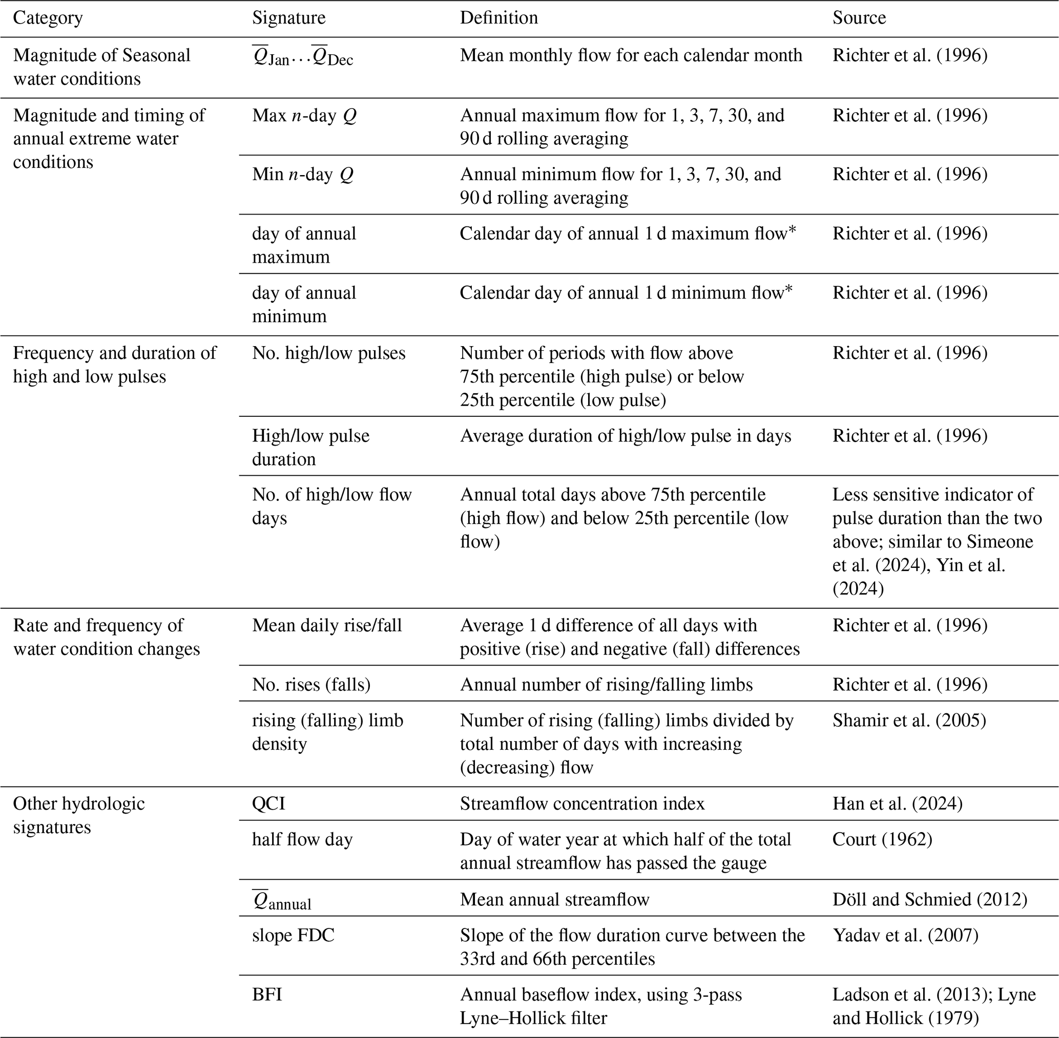
^∗ The water year is rotated to begin 183 d before the maximum (minimum) flow day, to prevent artificially large disagreements between simulated and observed time series arising from maximum or minimum flow dates occurring just before or just after the beginning of the water year.

2.3.2 Simulated changes in hydrologic signatures

The NSEs for the interannual, seasonal, and irregular components provide a concise and holistic summary of performance for each type of variance. However, studies of hydrologic change are often concerned with predicting changes to hydrologic signatures relevant to ecology or water management, so it is useful to evaluate how well models simulate changes in these signatures over the historical period. To this end, we compared simulated and observed values of 41 hydrologic signatures calculated on an annual basis (Table 1). The ecologically-relevant signatures that we consider are the 32 indicators of hydrologic alteration proposed by Richter et al. (1996) in addition to the total number of days below the 25th percentile (Number of low flow days), the total number of days above the 75th percentile (Number of high flow days), the rising and falling limb densities, the streamflow concentration index, the half flow day, the mean annual flow, the slope of the midsegment of the flow duration curve, and the baseflow index (see Table 1 for references). These additional metrics have been widely used by hydrologists to characterize hydrologic regimes and to detect trends.

We are interested in whether the hydrologic models accurately reproduce interannual variability in these 41 signatures, so we calculated non-parametric correlation coefficients between the simulated and observed annual series of hydrologic signatures, using Spearman's ρ for most metrics. Two metrics (No. high pulses and No. low pulses) frequently have tied ranks, so for these we used Kendall's τ.

We also calculated five other popular performance metrics that evaluate interannual, seasonal, and irregular variance jointly: the KGE^′, KGE^′ ($\mathrm{1}/Q$), and the three components of the KGE^′: Pearson r, the mean bias β and the ratio of coefficients of variation γ (Kling et al., 2012). To be consistent with the other metrics (for which values near 1 are better), we transformed β and γ to the range $(-\mathrm{\infty },\mathrm{1}]$ using the transforms $(\mathrm{1}-\sqrt{(\mathit{\beta }-\mathrm{1}{)}^{\mathrm{2}}})$ and $(\mathrm{1}-\sqrt{(\mathit{\gamma }-\mathrm{1}{)}^{\mathrm{2}}})$. These transforms are analogous to the use of these terms in the KGE.

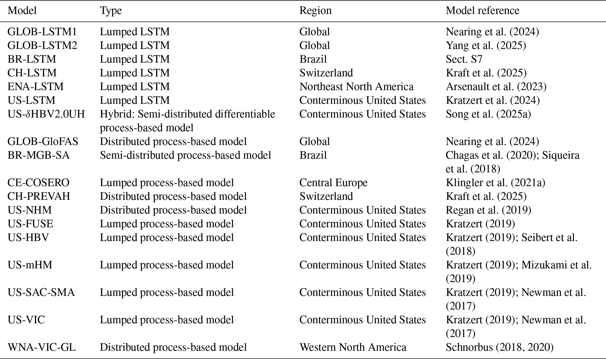
Table 2 18 models for which we reanalysed simulations to test performance on interannual, seasonal, and irregular variance components.

We applied the same tests here as for the variance component NSE values (Sect. 2.3.1): we compared the values of each metric between the highly seasonal and less seasonal subsets using Mann–Whitney U-tests. We also performed the same analysis after splitting the catchments based on thresholds of 0.4 and 0.6 for the seasonal variance fractions, and splitting on the streamflow concentration index (Han et al., 2024), the coefficient of variation of the average hydrograph, the aridity seasonality, and the fraction of precipitation as snow (Knoben et al., 2018).

3 Data

3.1 Streamflow Data

We compiled streamflow data from 16 CAMELS-type datasets from Australia (Fowler et al., 2024), Brazil (Chagas et al., 2020), Central Europe (Klingler et al., 2021a), Chile (Alvarez-Garreton et al., 2018a), Denmark (Liu et al., 2025), France (Delaigue et al., 2025a), Germany (Loritz et al., 2024), Great Britain (Coxon et al., 2020a), Iceland (Helgason and Nijssen, 2024a), India (Mangukiya et al., 2025a), Israel/West Bank/Golan Heights (Efrat, 2025), Luxembourg (Nijzink et al., 2024), the United States (Addor et al., 2017; Newman et al., 2015), North America (Arsenault et al., 2020), Spain (Casado Rodríguez, 2023), and Switzerland (Höge et al., 2023). For countries not represented in the above datasets we used streamflow data from the Global Runoff Data Centre (GRDC, https://grdc.bafg.de/, last access: 11 March 2025). We also added data from 138 Russian stations (Lammers and Shiklomanov, 2000) and ensured they were not duplicates of the GRDC stations. In total we compiled records from 28 406 stations worldwide.

3.2 Streamflow Simulations

We searched Google Scholar and used ChatGPT to identify freely available datasets of simulated streamflow at gauged locations. We required that some of the gauges be in the tropical, alpine, or polar regions where we expect the seasonal variance fraction to be high. Where publications reported the results of multiple versions of the same or very similar models, we selected the version identified by the authors as having the best performance.

In total we compiled simulations from 18 models this way: six Long Short-Term Memory Models (LSTMs), eleven process-based hydrologic models, and one hybrid model. These models are listed in Table 2, and Table S1 in the Supplement provides more extensive details about the calibration procedures for each model and the degree of human alteration of the catchments.

Where possible we included only near-natural catchments in the evaluation of each model, either as defined by the authors or by referencing other published lists of near-natural catchments (Falcone, 2011; Newman et al., 2015; Pellerin and Nzokou Tanekou, 2020). For the two Brazilian models, we used only catchments without regulation, with less than 5 % impervious surfaces, and consumptive use less than 5 % of annual streamflow. For the two global models published by Nearing et al. (2024) we included all available catchments since we lacked a reliable way to identify near-natural catchments.

Where models used a split-sample approach to training and testing we used the testing subset. The type of split sample is listed in Table S1. Some models were tested in unseen catchments, some were tested in unseen time periods, and some did not employ a split-sample approach or did not provide sufficient detail to determine which subset of the simulation data was not seen during training/calibration. Six of the models (CE-COSERO, US-FUSE, US-HBV, US-mHM, US-SAC-SMA, and US-VIC) were basin-calibrated, while the rest were globally calibrated.

4 Results and Discussion

4.1 Global Distribution of seasonal, interannual and irregular variance

Figure 1a shows the fraction of variance associated with seasonal, interannual, and irregular variance for 17 245 catchments. Globally, irregular variance dominates: more than half the variance is irregular in 70 % of the catchments. Figure S19 in the Supplement shows histograms of each variance fraction.

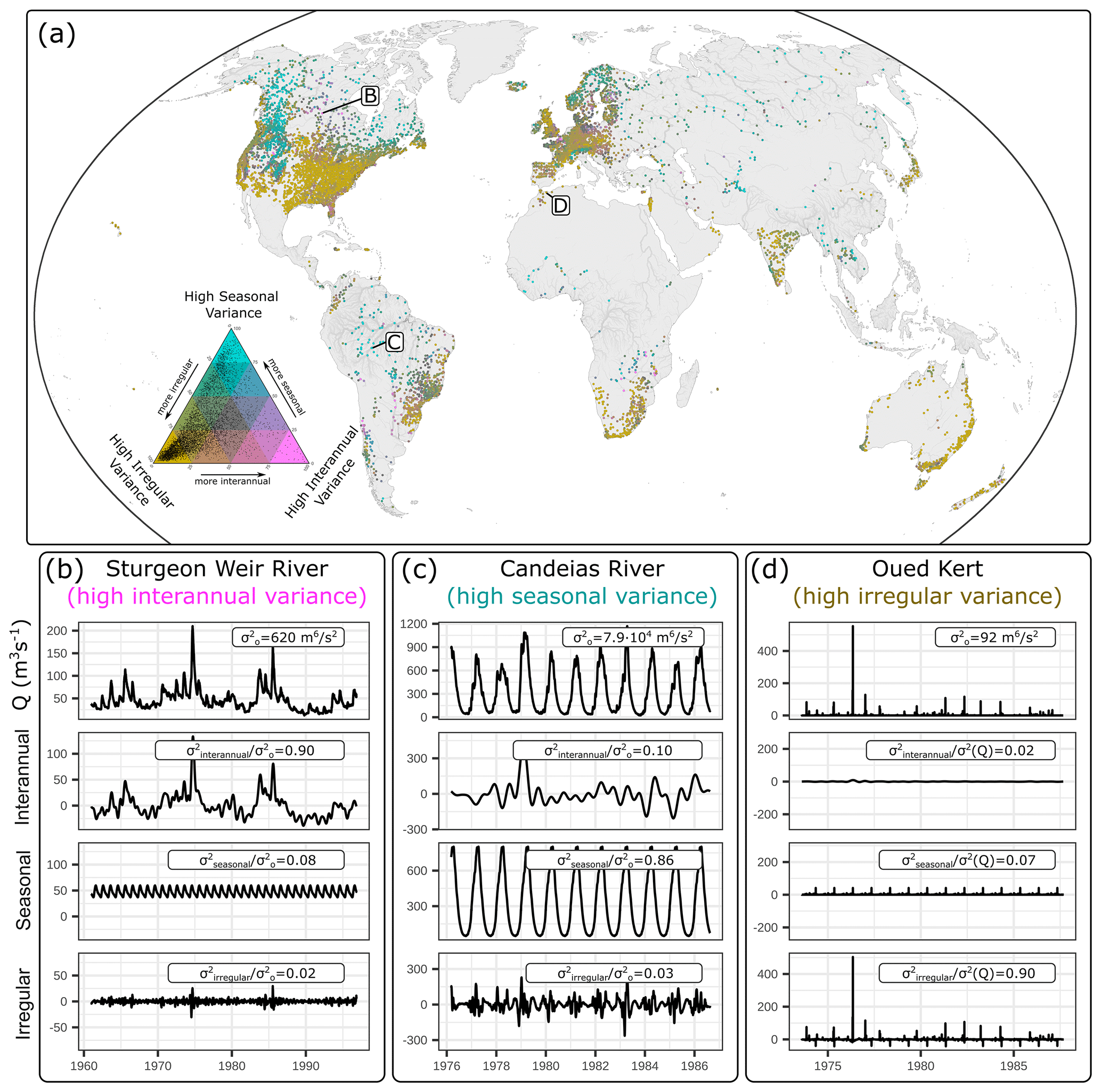
Figure 1 (a) The fraction of variance that is seasonal, interannual, and irregular. To reduce overplotting, gauges have been aggregated to 1 per 2500 km² using the mean of each variance fraction. (b)–(d) show the decomposed time series for three example rivers that exhibit high variance fractions for each of the three components. (b) The Sturgeon Weir River at the outlet of Amisk Lake (Water Survey of Canada ID 05KG002, catchment area 14 600 km²), an interannually variable stream (90 % interannual variance). (c) Santa Isabel (Candeias River at Candeias do Jamari, Agência Nacional de Águas e Saneamento Básico ID 15550000, catchment area 12 700 km²), a highly seasonal stream (86 % seasonal variance). (d) Oued Kert at Driouch, an ephemeral stream in Morocco (Global Runoff Data Centre ID 1304800, catchment area 1353 km²), where 90 % of the variance is irregular. The mapped river network is derived from HydroRIVERS v1.0 (Lehner and Grill, 2013).

Streams in arid regions (such as the ephemeral Oued Kert in Morocco, Fig. 1d) are especially irregular, because the streamflow time series are composed of infrequent flash floods driven by episodic heavy rainfall (D'Odorico and Bhattachan, 2012; Smith et al., 2015). However, flashy catchments in humid regions can also have high irregular variance fractions. Additional examples of highly irregular streams are included in Figs. S26–S31, from arid catchments in Telangana (India), New Mexico (USA), and Kunene (Namibia), and humid catchments in Newfoundland (Canada), Narvik (Norway) and Westland (New Zealand).

Highly seasonal catchments (those with a seasonal variance fraction above 0.5) are found primarily in cold (polar and alpine), and tropical climates, where seasonality is driven either by snow accumulation and melt or by strong monsoons. Figure 1c shows the Candeias River, a highly seasonal tropical catchment with some variation from year to year. The seasonal variance fraction is very high (greater than 0.8) in only 1 % of catchments, but these extremely seasonal catchments are found on all continents except Oceania. Extremely seasonal catchments are found in the Arctic regions of Nunavut, Nunavik, Iceland, Sápmi, and Siberia, the alpine ranges of western North America, Europe, southern Patagonia, and central Asia, and the tropical Orinoco, Amazon, Niger, Congo, Irrawaddy, and Mekong basins. Additional examples of decomposed time series from extremely seasonal cold and tropical catchments are provided in Figs. S32–S38.

High interannual variability is rare and occurs mainly in catchments with large surface or groundwater storage and/or strong connections to climate oscillations. Figure 1b shows the decomposition for the Sturgeon Weir River in northern Canada, where strong connections to the Arctic Oscillation drive decadal-scale variability (St. Jacques et al., 2014) and seasonal as well as irregular variation is dampened by a large lake. Other regions with high interannual variance are: (i) semi-arid north-central Chile (e.g., Fig. S19), where warm phases of El Niño Southern Oscillation (ENSO) are associated with heavy rainfall, including major floods in 1997 (Araya et al., 2022), (ii) the Paraguay River Basin (e.g., Fig. S22), where interannual persistence in dry and wet conditions is linked to the extensive Pantanal (wetland) hydrology as well as ENSO, the Pacific Decadal Oscillation, and the Atlantic Multidecadal Oscillation (Santos and Slater, 2025), and (iii) southeastern England and northwestern France (e.g., Fig. S20), where variability is driven by the North Atlantic Oscillation (Rodwell et al., 1999; West et al., 2022), and the occurrence of record flooding from 2000–2001 (Marsh and Dale, 2002). Anthropogenic impacts also have the potential to cause interannual variability, such as in the Syr Darya (Kazakhstan) where water abstraction increased beginning with the expansion of irrigation canals in 1973 (Zou et al., 2019) (Fig. S25). The preceding examples are selected to illustrate the diverse drivers of interannual variability around the world. In-depth analysis of their hydrologic conditions is considered out of scope for this work.

Hydrologic models should be capable of simulating all three variance components, but accurate simulation of interannual variance is arguably the most important when the objective is to predict long-term changes in statistical properties of streamflow, such as for climate change impact research. Accurately simulating interannual variance is probably an easier task in catchments that have historically been very interannually variable (such as the Sturgeon Weir River) than it is in catchments that have been interannually stationary, because there is more variance with which to calibrate hydrologic models. Nevertheless, historically stationary regimes are not guaranteed to remain stationary, so we believe this difficult task is worthwhile (Gudmundsson et al., 2012; Milly et al., 2008; Safeeq et al., 2014).

4.2 Out-of-sample climatological benchmark NSE (NSE_cb)

Figure 2a shows the NSE_cb for 20 338 catchments, based on leave-one-out cross-validation. Overall, the median is small with a value of 0.11, which implies that streamflow in most catchments is largely unpredictable based only on climatology from other years. On the other hand, the NSE_cb is high (greater than 0.5) for 10 % of the gauges. We argue that special care is warranted when modelling these catchments to ensure they add information beyond what is contained in the climatology.

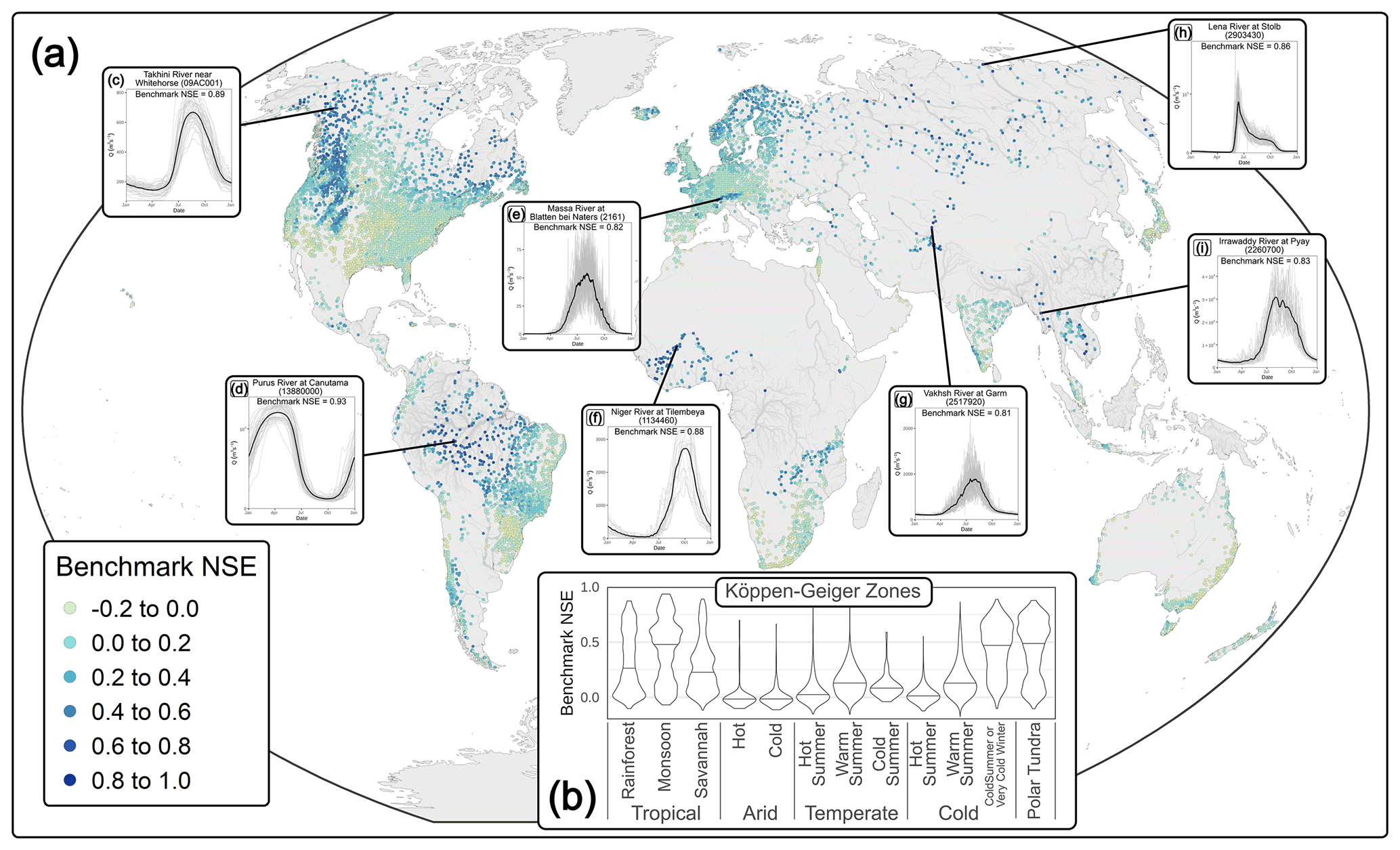
Figure 2 (a) Climatological benchmark Nash–Sutcliffe Efficiencies for 20 338 catchments. To reduce overplotting, for panel (a) gauges have been aggregated to 1 per 2500 km² using the median NSE. (b) Distribution of the climatological benchmark NSE by Köppen–Geiger climate zone. Cold (high alpine and polar) and tropical climates have high benchmark NSE values, often upwards of 0.5 and occasionally upwards of 0.8. (c–i) Annual hydrographs from catchments with very high benchmarks (BNSE > 0.8). The grey lines are individual years and the solid black line is the mean flow for each calendar day. The mapped river network is derived from HydroRIVERS v1.0 (Lehner and Grill, 2013).

Figure 2b shows that high NSE_cb values tend to occur in tropical monsoon and cold/polar Köppen–Geiger climate zones. Figure 2c–i show hydrographs from several catchments with NSE_cb > 0.8, from arctic, alpine, and tropical locations. Very high NSE_cb values do rarely occur elsewhere, although we note that some of these catchments are large and cover multiple climate zones. For example, the Mekong and Irrawaddy are classified as “temperate” based on catchment average climate data, but they are more accurately described as a mix of polar climate zones (at their headwaters in the Tibetan Plateau), temperate zones through their midsections, and tropical zones nearer to the gauging stations.

Figure S1 shows the ${\mathrm{KGE}}_{\mathrm{cb}}^{\prime }$ for the 20 338 catchments. The patterns are very similar to those seen with the NSE_cb, and Sect. S1 shows that ${\mathrm{KGE}}_{\mathrm{cb}}^{\prime }$ and NSE_cb are uniquely and monotonically related if no cross-validation scheme is used. After implementing the leave-one-out cross-validation scheme, this relationship is modified by the number of years of data. Thus, in this article we focus on the NSE_cb but we point out that the ${\mathrm{KGE}}_{\mathrm{cb}}^{\prime }$ behaves similarly.

The cross-validation scheme ensures the climatological model is always tested on unseen data, but a more difficult test is the differential split sample, where models are tested on data outside of their calibration conditions. This has been widely applied and recommended to test models used for climate change impact assessment (Klemeš, 1986; Krysanova et al., 2018; Refsgaard et al., 2014; Seibert, 2003). In Sect. S9 we show that the NSE_cb remains high in tropical, alpine, and polar catchments when evaluated using a differential split sample methodology. The climatological benchmark model is, by definition, unable to simulate interannual variance or change, so the fact that it can achieve high NSE values when tested on data outside of its calibration conditions further reinforces that high NSE values do not guarantee a model is useful for making hydrologic predictions under climate change.

This is, to the best of our knowledge, the largest and most geographically extensive compilation of benchmark performance values for streamflow gauging stations to date. Figure 2 serves as a reminder the NSE is not an absolute measure of performance, and that comparing NSE values across catchments is challenging, because baseline performance varies substantially (Knoben, 2024; Martinec and Rango, 1989; Schaefli and Gupta, 2007; Seibert, 2001). Our analysis builds on previous work by showing that NSE_cb can be high even when evaluated on unseen data. In this work, however, we are primarily interested in analysing if the ease of achieving high NSE scores in some catchments jeopardizes the modelling of interannual variance. This is the subject of the following section.

4.3 High NSEs can hide poor representations of interannual variance

4.3.1 Variance component NSE values

Figure 3 shows that high NSE values often hide inferior simulations of interannual and irregular variability. The overall NSE is consistently higher in highly seasonal catchments, but this is mainly driven by an improvement in modelling the seasonal component (NSE_seasonal). NSE_interannual values are lower in highly seasonal catchments for all models except GLOB-GLOFAS (where the median NSE_interannual value is near zero for both highly seasonal and less seasonal catchments), and WNA-VIC-GL. NSE_irregular values are also usually lower in highly seasonal catchments.

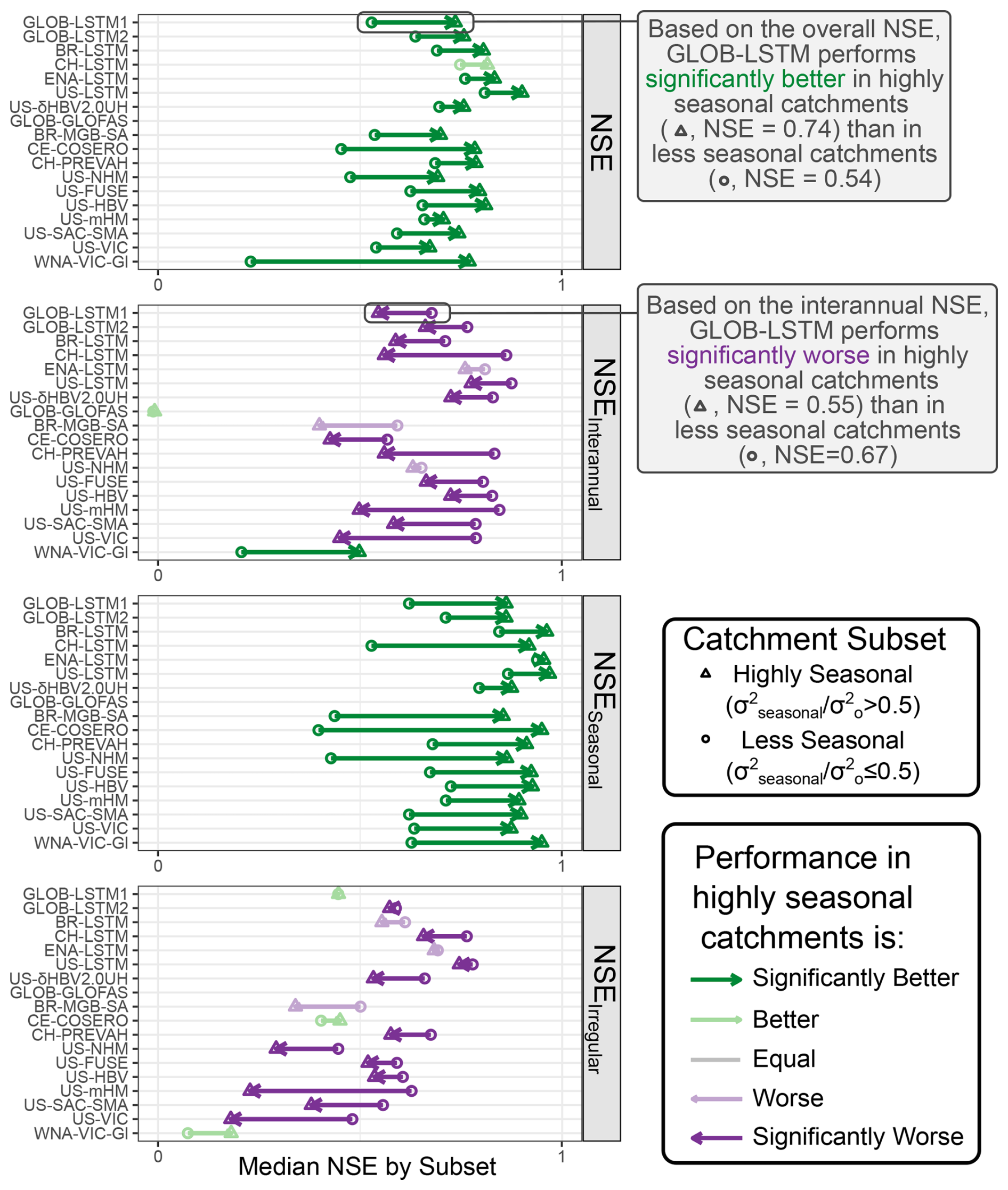
Figure 3 Comparison of NSE scores between highly seasonal and less seasonal catchments, across 18 hydrologic models (vertical axis labels correspond to Table 2). For all models the NSEs of the overall time series and of the seasonal component are better in highly seasonal catchments, but the NSEs of the interannual and irregular components are usually significantly worse. The arrows point from the median value for less-seasonal catchments to the median value for highly seasonal catchments. Significance is determined at p < 0.05 using the unpaired Mann–Whitney U-test. The median NSE was negative for GLOB-GLOFAS for all components and subsets.

One might expect that higher NSEs can be achieved in highly seasonal catchments because seasonal variability is easy to model, and there is more of it. However, Fig. 3 suggests this is only part of the story: in highly seasonal catchments there is more seasonal variance, and a larger fraction of it is modelled accurately (NSE_seasonal is larger).

4.3.2 Simulated changes in hydrologic signatures

Figure 4 shows the expanded analysis for 6 typical performance metrics and 41 interannual signature metrics (see Table 1). The typical metrics (top row) are higher in highly seasonal catchments. NSE, KGE^′, Pearson r, and variance ratio γ are better in highly seasonal catchments across all 13 models, and most of these differences are statistically significant. KGE^′ ($\mathrm{1}/Q$) shows a similar pattern except for some of the process-based models for the United States, which struggle to simulate winter low flows in colder regions.

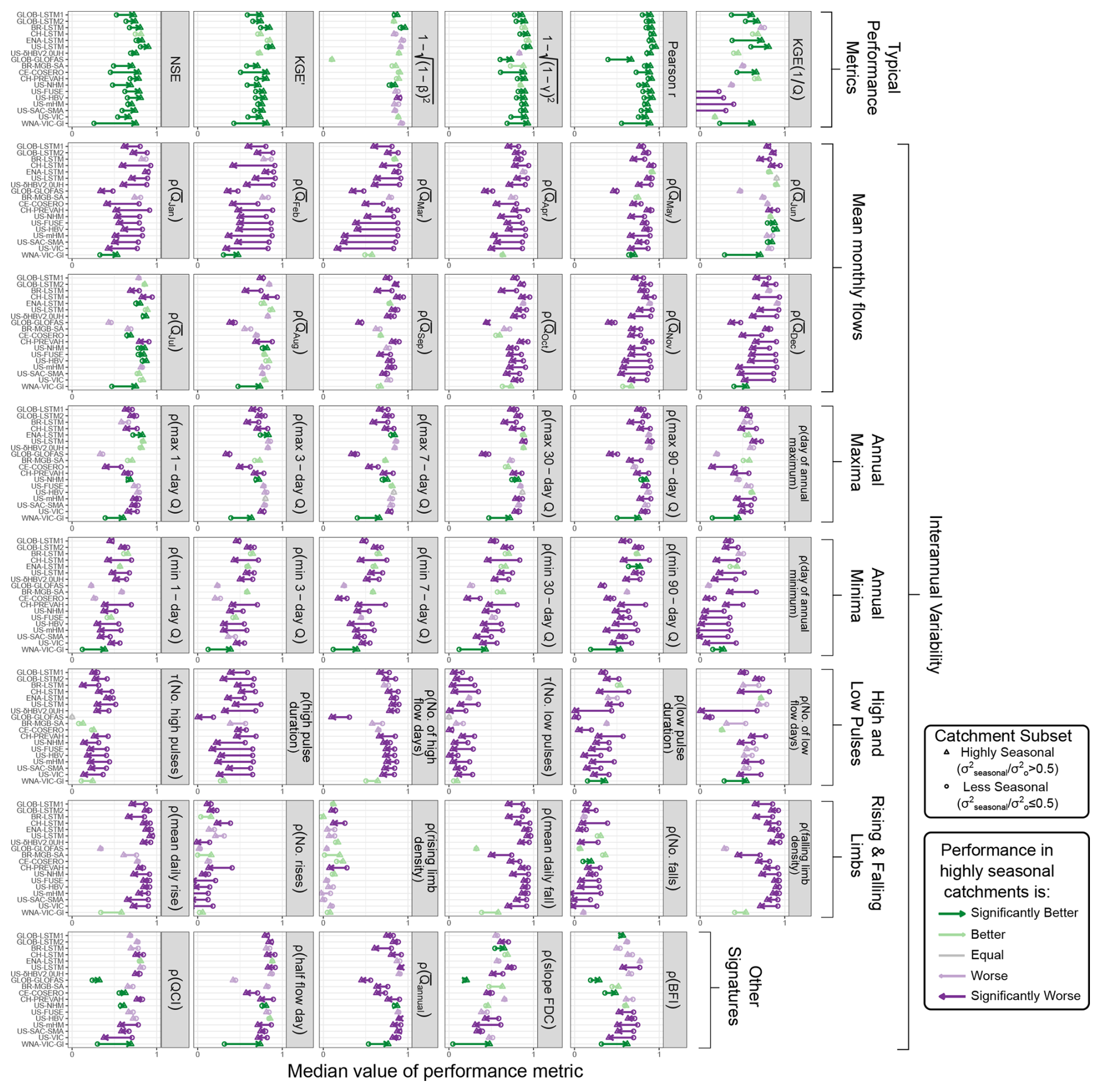
Figure 4 Catchments in high-benchmark NSE regions generally perform better than low-benchmark catchments on typical performance metrics which combine intra and interannual variance (top row) but are significantly worse when evaluated on other metrics that focus on interannual variability. The arrows point from the median value for low-benchmark catchments to the median value for high-benchmark catchments. Significance is determined at p < 0.05 using the unpaired Mann–Whitney U-test. Note that the median NSE, KGE^′, and KGE^′ ($\mathrm{1}/Q$) are negative for GLOB-GLOFAS in both highly seasonal and less seasonal catchments.

In the seasonal catchments where typical performance metrics are high, we again see that interannual variability is more poorly simulated: the correlations between observed and simulated annual values of 41 hydrologic signatures across 13 models are worse in highly seasonal catchments for 80 % of the cases (63 % at a significance level of p=0.05). All models except WNA-VIC-GL perform worse in highly seasonal catchments across most (> 50 %) of the interannual signature metrics, and all but one of these metrics are lower in highly seasonal catchments across most of the models.

Some of the differences in performance are quite large. For example, the Spearman rank correlations for monthly flows from November to April are close to 1 (perfect) for less seasonal catchments and below 0.5 for some models in highly seasonal catchments. The predictions of annual minima, high and low pulses, and rising and falling limbs are also substantially worse in highly seasonal catchments.

These non-parametric correlations test if the models correctly predict the direction of change, but not the absolute values of each signature. We also calculated the NSE of the simulated and observed annual series of hydrologic signatures, but all models struggle to simulate absolute values of at least some of these signatures: across 738 model-by-metric combinations, the NSE of the simulated hydrologic signatures is negative for both the highly-seasonal and less-seasonal subsets 48 % of the time (Fig. S11). We view large, positive correlations with historical observations as a minimum requirement to consider a model useful for simulating hydrologic responses to a changing climate.

In Sect. S6 we present various robustness tests of these results. We tried changing the splitting threshold (seasonal variance fractions of 0.4 and 0.6, instead of 0.5). Our analysis and conclusions are insensitive to these changes. We also tried splitting the catchments using the snow fraction, and for snow-dominated regions the results were similar to Fig. 4. Splitting on several indices did not produce clear patterns.

4.3.3 Causes of poor interannual performance

Our analysis does not directly identify the causes of poor interannual performance in highly seasonal catchments, but we hypothesize that model optimization algorithms, model structures, and data quality and quantity all play a role.

First, model optimization algorithms may bias training away from highly seasonal catchments. Seasonal variance is predictable and can be reproduced quite accurately with models of low complexity (Knoben, 2024). Where models are optimized simultaneously across many catchments, optimization algorithms may therefore greedily simulate the seasonal variance in seasonal catchments and neglect interannual and irregular variance. When seasonal variance is well-simulated, algorithms will prioritize improvements to modelling the irregular and interannual components in less-seasonal catchments where these improvements result in the largest increase to the average NSE. Learned human biases for what a “good” simulation looks like could also bias modellers to neglect catchments where errors appear small compared to the seasonal pattern, since expert opinions and current quantitative metrics have been shown to be mostly consistent (Gauch et al., 2023). However, six of the models that we analysed were calibrated individually to each catchment, so this explanation is not sufficient on its own.

Second, model structures often do not include important hydrologic components for highly seasonal catchments, such as glacier change, avalanching, and vegetation-moisture feedbacks (D'Odorico et al., 2007; Köplin et al., 2013; Staal et al., 2020). These components can be drivers of interannual variability and change, and we hypothesize that their inclusion could improve simulations of interannual variability.

Third, data quality and quantity are often lower in remote polar, alpine, and tropical regions. Long-term weather stations tend to be scarce in these regions, which means that the gridded meteorological data used to run models may not accurately capture interannual climate variability (Burton et al., 2018), and therefore interannual streamflow variability will also be poorly modelled. There are also few gauged streams in highly seasonal regimes globally (Krabbenhoft et al., 2022), and optimization algorithms that aim to maximize the average performance across many catchments will not prioritize improving simulations for a small number of highly seasonal catchments.

Indeed, the global distribution of stream gauges is very biased (Krabbenhoft et al., 2022), and highly seasonal catchments are underrepresented in the datasets we analysed. Cold climates with cold or very cold winters (as defined in the Köppen–Geiger climate classification by Beck et al., 2018) represent 15 % of global non-frozen lands (excluding perennially ice-covered regions but only 10 % of the catchments in our selected datasets, and polar tundra occupies 6.7 % of global land and just 2.4 % of catchments. The tropical zone is even more underrepresented: tropical rainforest and tropical monsoon climates represent 6.2 % and 4 % of global lands, and collectively generate 39 % of global runoff (based on Beck et al., 2018 and Ghiggi et al., 2019), but only 0.9 % and 0.8 % of catchments in our datasets are located in these zones, respectively.

Other compilations of streamflow data are even more biased, particularly in underrepresenting tropical regions. Caravan, a popular compilation of 6830 catchments (Kratzert et al., 2023), included only 8 tropical rainforest and 5 tropical monsoon catchments in its initial version. Several “community extensions” (e.g., underline Färber et al., 2025) have improved the global coverage of the Caravan project, but the distribution remains highly biased. Another initiative, the Reference Observatory of Basins for INternational hydrological climate change detection (ROBIN), includes streamflow data and catchment polygons for 2265 near-natural streams worldwide, but only 19 tropical rainforest and 6 tropical monsoon catchments Turner et al., 2025).

Our understanding of hydrologic processes and change in highly seasonal regimes is thus impeded not just by poor modelling of interannual variability, but also by the underrepresentation of these regimes in the datasets that are currently available and widely used in the hydrological modelling community. Efforts to increase the representation of these regimes could include making existing data publicly available e.g., Lin et al., 2023), digitizing paper records (e.g., Bathelemy et al., 2024; Henck et al., 2011), or installing new stream gauges. However, we acknowledge that at least some of the causes of global gauge biases are not easily overcome (Krabbenhoft et al., 2022), and that we must continue to rely on approaches to predictions in ungauged basins (Hrachowitz et al., 2013).

5 Conclusions and Recommendations

Streamflow time series are made up of interannual, seasonal, and irregular components, and models can perform very differently with respect to these three components. These differences are obscured when aggregated performance metrics such as NSE and KGE are used. Our findings have several relevant consequences.

First, we provide further evidence that using the same performance thresholds to judge hydrological models across catchments is ill advised. Especially in tropical, alpine, and polar climates it is generally easier to achieve high NSE values: the climatological benchmark NSE_cb is often higher than 0.5 and occasionally even higher than 0.8. We observe, in Figs. 3 and 4, that hydrologic models do achieve higher NSE and KGE values in these highly seasonal, high-benchmark catchments. It is therefore important to contextualize model performance with climatological and other benchmark models (Knoben, 2024).

Second, it is critical to choose evaluation metrics that are suitable for both the study location and model purpose. We show that high NSE values often hide inferior simulations of interannual variance, including changes in ecologically relevant hydrologic signatures. This is most evident in tropical, alpine, and polar regions, where most of the variance in streamflow is seasonal. Poor interannual performance in these regions (and in some cases almost complete failure to simulate year-to-year variability) raises concerns about the ability of these models to accurately simulate nonstationary hydrologic processes and responses to climate change. This is especially worrying because these regions may be some of the most vulnerable to climate change (Flores et al., 2024; Pepin et al., 2022; Rantanen et al., 2022) and are historically less-well studied regarding hydrologic extremes (Stein et al., 2024). We recommend that authors evaluate how well models simulate interannual variance to understand how well a model may extrapolate to different locations or climate conditions.

We encourage the community to pay more attention to interannual variance and to the highly seasonal regimes where it is most poorly modelled. This could include developing new calibration targets and objective functions to train models that improve the representation of interannual variance. Some suitable calibration targets include the interannual NSE introduced in Sect. 2.3, and the correlations of the hydrologic signatures in Table 1. Lastly, we stress the need to collect and publish observations from more tropical, alpine, and polar regions, which are underrepresented in global datasets.