Benchmarking historical performance and future projections from a large-scale hydrologic model with a watershed hydrologic model

Large-scale hydrologic models (LHMs) are increasingly relied upon for assessing climate-driven hydrologic changes from watershed to global scales. However, their ability to provide robust projections for a range of hydrologic variables remains unclear. Here, we evaluate the historical performance and future projections from the Community Water Model (CWatM) LHM against the Variable Infiltration Capacity (VIC) watershed hydrologic model for the Liard River basin (drainage area of ∼ 275 000 km²) in subarctic Canada. The model setups have key differences in terms of model configuration (CWatM is set up with two subbasins, and VIC is set up with 28 subbasins) and model structure (e.g., snowmelt and frozen soil representation). We drive both models with an ensemble of eight global climate models from the Coupled Model Intercomparison Project Phase 6, downscaled and bias-corrected with a multivariate method. We analyze a range of hydrologic projections at 1.5 to 4.0 °C global warming levels (GWLs) above the preindustrial period. The historical performance benchmarking shows reasonable goodness-of-fit metrics for both models, with a slightly better performance for VIC. Projected hydrologic responses from CWatM are generally consistent with VIC in terms of annual water balance, as well as monthly snow water equivalent and flow changes, suggesting the robustness of the projections. Both models project coherent hydrologic changes, including progressively higher annual evapotranspiration; increased annual, winter, spring, and maximum flows; increased frequency of extreme flow; and earlier timing of maximum flow, with higher GWLs. However, the magnitudes of maximum flow and late-summer flow diverge between the two models, which can be explained by structural uncertainties associated with the representation of frozen soil and groundwater processes. Thus, our study provides insights into the robustness of hydrologic projections from an LHM and offers a basis for model improvements.

1 Introduction

Hydrologic models are essential tools for assessing historical and future changes in water cycle variables from a watershed to regional and global scales. It is a common practice to employ watershed-scale hydrologic models for assessing the impacts of anthropogenically driven change, such as land use, riverine change and climate change (e.g., Byun et al., 2019; Chegwidden et al., 2019; Eum et al., 2016; Shrestha et al., 2019). In recent years, global water models have increasingly been relied upon for assessing the past or present changes and for projecting future changes in hydrological variables from regional to global scales (e.g., Döll et al., 2018; Krysanova et al., 2020; Pokhrel et al., 2021; Greve et al., 2023).

Global water models broadly originate from the climate science community as land surface models, from the global hydrology and water resources community as global hydrologic models (GHMs), and from the vegetation and carbon modelling community as dynamic vegetation models (Bierkens, 2015; Telteu et al., 2021). Particularly, GHMs are closely related to watershed hydrologic models (WHMs) in terms of modelling philosophy and functionality but may differ with WHMs in physical process representation and spatial discretization. Specifically, GHMs are generally designed to provide consistent simulation of the water cycle components at continental or global scales with a simplified representation of physical processes (Hattermann et al., 2017; Veldkamp et al., 2018). In contrast, WHMs typically include more sophisticated and complex process representations that are often tailored to the specific characteristics of a watershed or river basin. In terms of spatial discretization, WHMs offer finer resolution (typically ≤ 10 km) than GHMs (typically 0.5° × 0.5° or ∼ 50 km × 50 km at the Equator), allowing for greater topographic complexity. The two modelling approaches may also differ in terms of model parameterization, with GHMs generally parameterized to represent large-scale processes and not calibrated to watershed-specific conditions, whereas WHM parameters are calibrated using river discharge and other available observations, e.g., snow water equivalent and evaporation (Krysanova et al., 2020). These differences could cause GHM-simulated responses to diverge from observations and WHM simulations, especially in replicating extreme maximum and minimum flows (Zaherpour et al., 2018; Heinicke et al., 2024). In northern regions, some GHMs may perform poorly due to the lack of representation of cold-climate processes (Gädeke et al., 2020).

These limitations are being addressed through ongoing enhancements in the GHMs (Bierkens, 2015; Telteu et al., 2021). For example, improvements in physical process representation have resulted in a more reasonable reproduction of monthly and seasonal streamflow dynamics, as well as extreme flows (Huang et al., 2017; Veldkamp et al., 2018). Calibration of GHMs against observations (e.g., streamflow and evaporation) has also led to improvements in model performance (e.g., Zaherpour et al., 2018; Burek et al., 2020; Döll et al., 2024). Furthermore, parameterization of GHMs using regionalization methods has also improved their performance (e.g., Beck et al., 2016; Qi et al., 2022; Yoshida et al., 2022). Additionally, finer spatial resolutions of 5 arcmin or less are becoming more common in GHMs (e.g., Burek et al., 2020; Hanasaki et al., 2022; van Jaarsveld et al., 2024). Thus, the distinction between the GHM and WHM when applied at a large river basin scale is diminishing, and more consistent hydrological assessments from river basin to regional and global scales is being facilitated. In this respect, GHMs, when applied at river basin scales, have also been referred to as large-scale hydrologic models (LHMs) (Merz et al., 2022; Hanus et al., 2024). However, key differences between the two modelling approaches may remain in terms of model configuration, e.g., LHMs are usually configured over entire river basins, whereas WHMs are usually configured with multiple subbasins. Furthermore, differences in physical process representation, especially dominant processes in a basin, may results in differences in hydrologic responses.

In this respect, as suggested by Beven (2023), a fit-for-purpose benchmarking to consider the suitability of a hydrologic model structure prior to a specific application is highly relevant. Benchmarking LHMs prior to watershed-scale or regional applications is also important as these models are designed to represent large-scale hydrologic processes and are not tailored to specific hydrologic conditions. There is, of course, no guarantee that a model that performs well for the historical climate will provide reliable future projections (Krysanova et al., 2020). However, it could be argued that an LHM's ability to replicate future simulations of a WHM increases the confidence in LHM-based projections.

Here, we present a benchmarking study that assesses the robustness of hydrologic responses from an LHM in comparison to a WHM in the context of climate change impacts. We focus on two key research questions. (1) Can an LHM, set up at a river basin scale, replicate the historical simulations and future projections from a WHM, configured with multiple subbasins? (2) How do the structural differences between the two modelling approaches affect the magnitude and direction of the projected hydrologic response? To address these questions, we set up the Community Water Model (CWatM) (Burek et al., 2020) as an LHM and the widely used Variable Infiltration Capacity (VIC) (Liang et al., 1994; Hamman et al., 2018) as a WHM for the Liard River basin in subarctic Canada. We drive both models with an ensemble of eight global climate models (GCMs) that participated in the Coupled Model Intercomparison Project Phase 6 (CMIP6) experiment (Eyring et al., 2016), downscaled and bias-corrected with the multivariate bias correction algorithm (MBCn; Cannon, 2018). After benchmarking a set of statistical goodness-of-fit metrics of CWatM and VIC simulations, we analyze the robustness of a set of projected hydrologic responses, including annual water balance, monthly flow, snow water equivalent, annual maximum flow and timing, and flood frequencies. We compare the range, magnitude and direction of changes, as well as agreement among ensembles, at the 1.5, 2.0, 3.0 and 4.0 °C global warming levels above the preindustrial period. Furthermore, this study updates CMIP5-based VIC model projections for the Liard River basin from previous studies (Shrestha et al., 2019, 2022).

2 Study basin

This study focuses on the Liard River basin (LRB), a large mountainous basin in northwestern Canada with a drainage area of approximately 275 000 km². The river's headwaters originate in the Cordillera mountains, with the drainage area covering parts of four Canadian provinces/territories: Yukon, British Columbia, Northwest Territories and Alberta (Fig. 1). The Liard River is a major tributary of the Mackenzie River, covering about 16 % of its drainage area and contributing about 25 % of discharge (Shrestha et al., 2019). Located in the subarctic zone, most of the basin is underlain by discontinuous permafrost (based on the classification by Heginbottom et al., 1995). The LRB is mostly in a pristine state, with very limited resource development and about 74 % forest coverage (Bonsal et al., 2020). Thus, the basin offers a good case for assessing the effects of LHM and WHM structures in simulating the cold-climate hydrologic regime, dominated by flows from snowmelt and frozen ground, and not affected by direct human impacts such as dams and reservoirs.

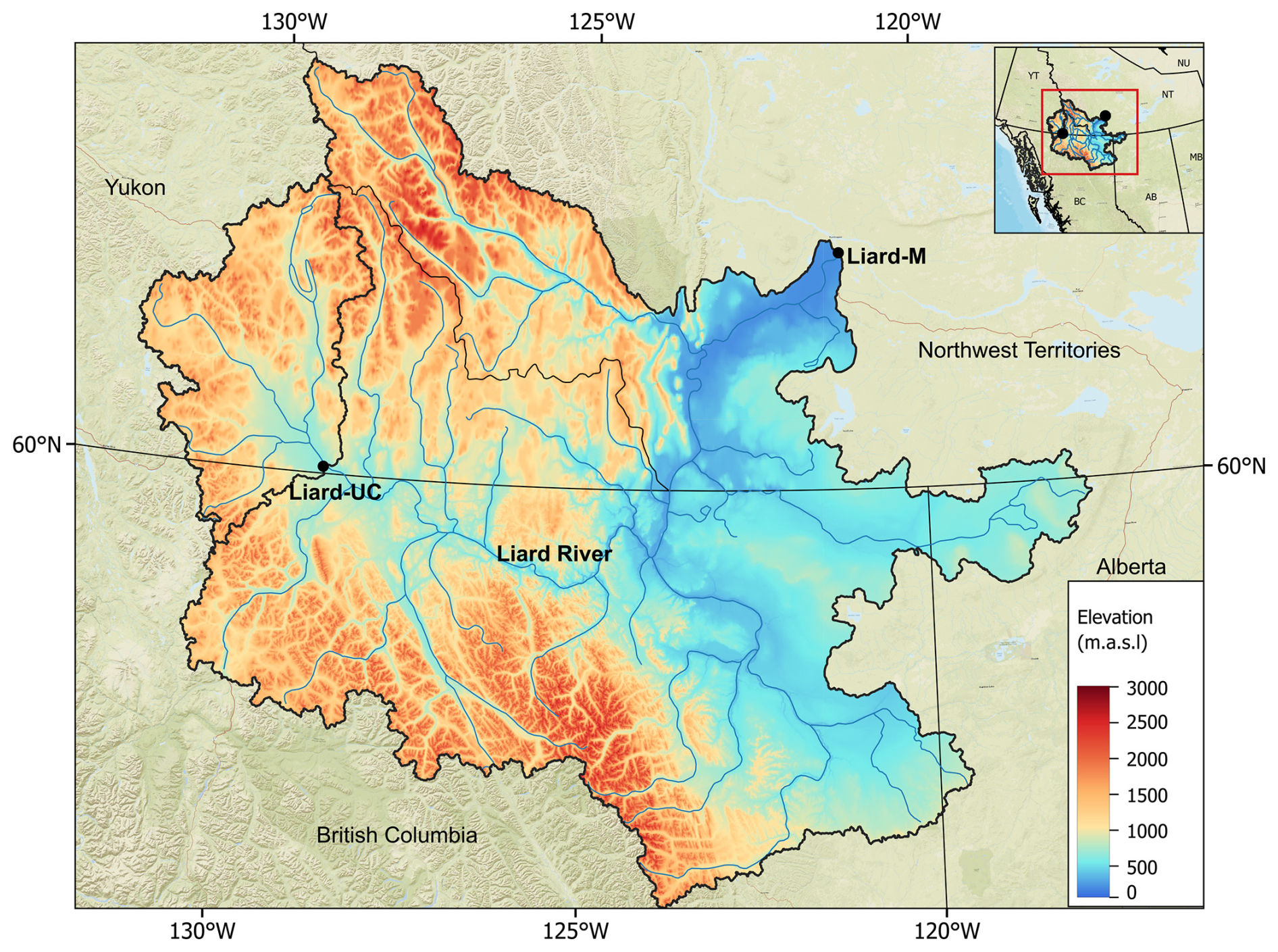
Figure 1 Location map of the Liard River basin. Also shown are the outlets of the Liard-M (Mouth) and Liard-UC (Upper Crossing) basins for which analyses were performed.

The mountainous topography of the region exerts a strong influence on the basin's climatology, particularly over the Cordillera mountains, creating a strong precipitation gradient (Szeto et al., 2008). The mean annual precipitation, temperature and runoff in the basin over the years 1979–2012 were about 570 mm, −2.0 °C and 290 mm, respectively (Shrestha et al., 2019). Seasonally, the basin receives a higher fraction of annual precipitation between April and September, while the runoff regime is dominated by snowmelt-driven high flows during the spring and summer months (Woo and Thorne, 2006). Annual air temperature and precipitation in the basin have increased by 2.2 °C and 12 %, respectively, over the years 1948–2016 (Bonsal et al., 2020). However, mean annual and maximum streamflow trends for most stations in the basin are negligible, except for the minimum flow increases (Shrestha et al., 2021).

3 Models, data and analyses

3.1 Hydrologic models

We employed the Variable Infiltration Capacity (VIC) hydrologic model version 5.0.0 (Liang et al., 1994, 1996; Hamman et al., 2018), set up at a $\mathrm{1}/\mathrm{16}$° spatial resolution for the LRB (Shrestha et al., 2019, 2022), as a benchmark WHM. VIC is a process-based, semi-distributed hydrologic model that accounts for sub-grid variability in snow and vegetation. Since its initial development in the 1990s, the model has undergone several updates and refinements. Especially the inclusion of key cold-region processes of energy balance over snow and frozen ground (Cherkauer and Lettenmaier, 1999, 2003; Andreadis et al., 2009) makes VIC suitable for the LRB; hence, VIC was considered a WHM. VIC has been used extensively for assessing the hydrologic impacts of climate change across cold-region river basins (e.g., Schnorbus et al., 2014; Eum et al., 2016; Chegwidden et al., 2019; Shrestha et al., 2019).

We compared the Community Water Model (CWatM) version 1.081, a large-scale, semi-distributed model developed for regional- to global-scale hydrologic applications (Burek et al., 2020), with the VIC model. Although CWatM was originally designed as a GHM, it has been adapted as an LHM with finer spatial resolution and model calibration setup. CWatM is not tailored for a specific region and developed with the philosophy of “as complex as necessary but not more” (Burek et al., 2020); it includes a simplified representation of cold-region processes, such as snow accumulation and melt and soil water movement through frozen soil. Similar to VIC, it accounts for sub-grid variability in snow and land cover. Furthermore, recent coupling of CWatM with a glacier model (Hanus et al., 2024) makes it suitable for cold-region applications, such as an assessment of impacts of climate change in glaciated watersheds. CWatM has been used for streamflow simulation in several global-scale assessments (Burek et al., 2020; Greve et al., 2020; Heinicke et al., 2024) and as part of a multi-GHM ensemble for future projections of floods, water shortage and drought (Boulange et al., 2021; Pokhrel et al., 2021; Satoh et al., 2022). However, to our knowledge, applications specifically focused on climate change impacts in cold regions are not available. For this study, we used the 5 arcmin (or $\mathrm{1}/\mathrm{12}$°) resolution CWatM configuration, including the static geospatial data made available by the model developers (ftp://rcwatm:Water1090@ftp.iiasa.ac.at/, last access: 3 June 2025).

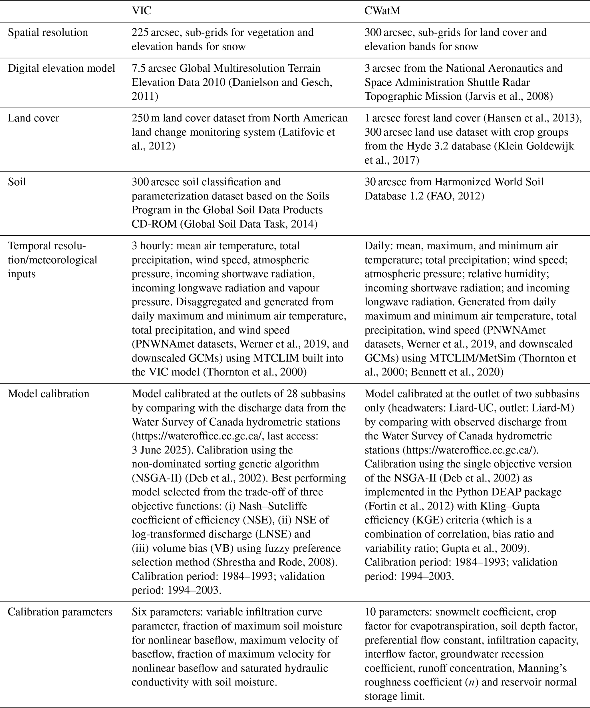
As summarized in Table 1, a major difference in the two model setups is the number of subbasins, with VIC configured as WHM by subdividing LRB into 28 subbasins and CWatM configured as an LHM by subdividing into 2 subbasins. While it is technically feasible to subdivide the CWatM setup to match the VIC subbasin structure, setting up and running it over 28 subbasins will be cumbersome, because, like most LHMs, CWatM is designed for large-scale applications and not for running over nested subbasins with multiple parameter sets. Note that VIC could also be set up as an LHM similar to CWatM. However, we wanted to apply these models as they were designed to be used – an LHM at the large basin scale and a WHM over multiple subbasins – and address research question 1. Nevertheless, we set up CWatM for the Liard River at the Upper Crossing (Liard-UC) subbasin to compare with the VIC model setup (Liard-UC is further subdivided into three subbasins in VIC) for a relatively small subbasin (drainage area = 32 600 km²). Besides the number of subbasins, the two model setups also differ in terms of spatial resolution and base geospatial datasets (soil, land cover and digital elevation model) (Table 1).

Table 1 Model resolution, geospatial and meteorological datasets, and model calibration for VIC and CWatM setups in this study.

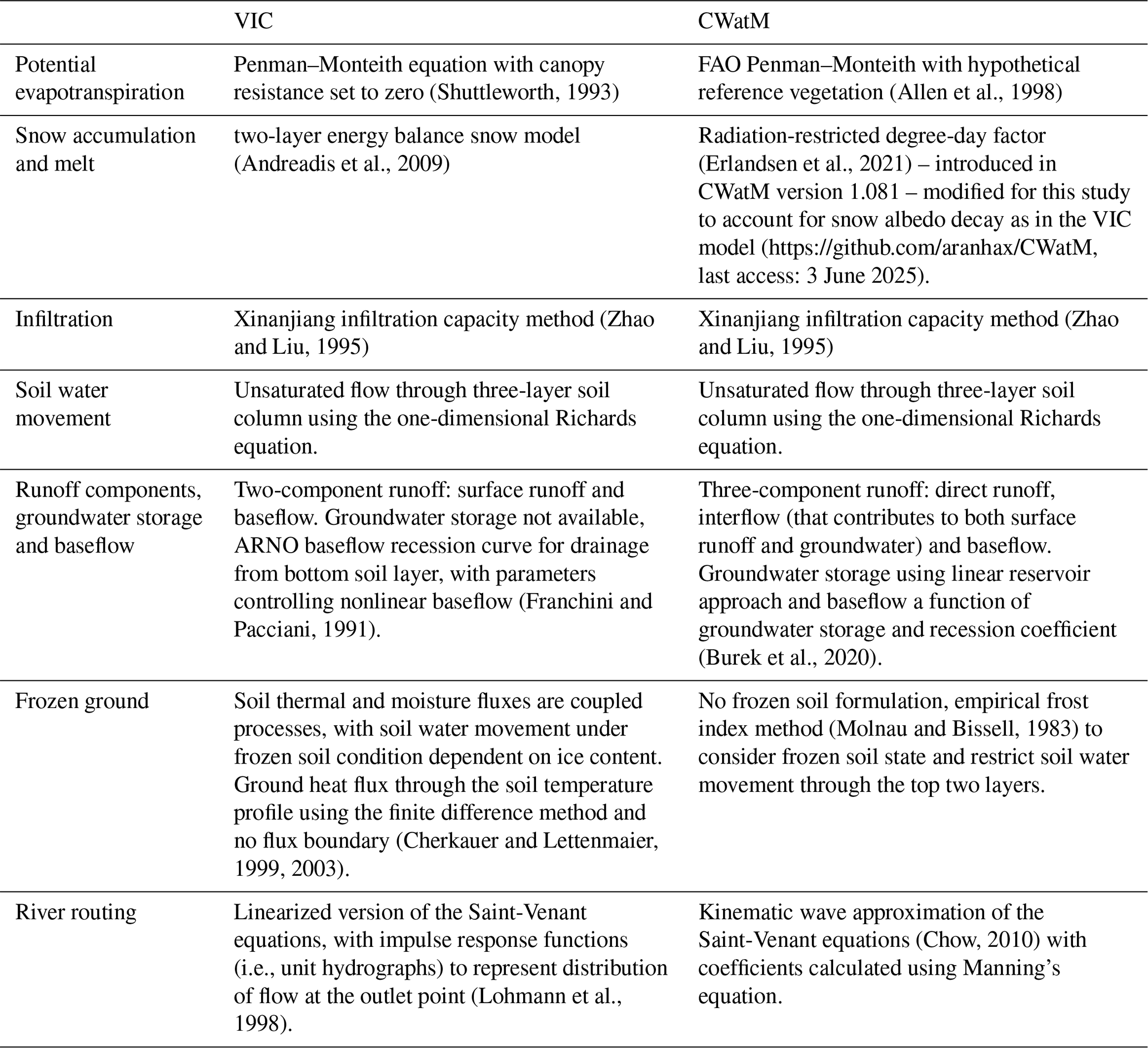
The representations of hydrologic processes in VIC and CWatM are mostly similar, except for subsurface flow, snow and frozen ground (Table 2). Specifically, the three-component runoff generation processes in CWatM, consisting of direct runoff, interflow and baseflow, differ from the two-component formulation in VIC, consisting of surface runoff and subsurface flow (baseflow). The presence of groundwater storage in CWatM can be expected to lead to delayed baseflow response compared to VIC without groundwater storage and baseflow response represented by a nonlinear function. Additionally, the representation of cold-region processes differs between the two models, with a full energy balance snow model and coupled soil thermal and moisture flux frozen ground model in VIC and with radiation-restricted snowmelt and frost index methods in CWatM. The differences in snowmelt methods could potentially lead to differences in snowmelt and runoff outputs. Finally, frozen soil methods control the soil water movement through frozen soil, and the differences can be expected to influence runoff generation pathways and consequently streamflow simulation. We considered these differences in VIC and CWatM structures for assessing effects on the magnitude and direction of hydrologic responses, according to research question 2.

Table 2 Summary of key physical process representation in VIC and CWatM as used in this study.

3.2 Climate data and downscaling

We used daily temperature, precipitation and wind speed from the Pacific North Western North America gridded meteorological data (PNWNAmet; Werner et al., 2019) as inputs for the calibration of both VIC and CWatM and as the target dataset for statistical downscaling (Table 1). PNWNAmet is a spatially contiguous and temporally consistent dataset spanning the years 1945–2012, which has been found to outperform other gridded observational data products available for the region in terms of climate means, extremes and variability, as well as streamflow trends and runoff ratios, when used to drive the VIC model (Werner et al., 2019). The PNWNAmet dataset has a spatial resolution of $\mathrm{1}/\mathrm{16}$°, matching the resolution of the VIC model used in this study.

We used an ensemble of eight CMIP6 GCMs (summarized in Table S1 in the Supplement) based on the GCM selection by Mahony et al. (2022) for the Intergovernmental Panel on Climate Change (IPCC) reference Northwestern North America region. The GCM selection methodology uses 10 different criteria, and the selected eight-model subset represents the very likely range of Earth's equilibrium sensitivity according to IPCC's recent assessment (Arias et al., 2021). For each GCM, we considered the historical period (1950–2014) and two shared socioeconomic pathways (SSPs), consisting of high (SSP5-8.5) and moderate (SSP2-4.5) scenarios over the years 2015–2100. Thus, uncertainties due to GCM structure, greenhouse gas concentration and anthropogenic forcing pathways – which are the most important sources of uncertainties in projecting hydrologic impacts of climate change (Hattermann et al., 2018; Chegwidden et al., 2019) – are considered in this study.

We employed a state-of-the-art N-dimensional probability density function transform and multivariate bias correction method (MBCn; Cannon, 2022, 2018) to spatially disaggregate and bias-correct coarse-resolution GCM outputs, consisting of daily precipitation, maximum and minimum temperature, and wind speed, to the $\mathrm{1}/\mathrm{16}$° resolution of the PNWNAmet dataset. This method preserves multivariate dependence of the target observational data, which is an important consideration for multivariate climate extremes (Zscheischler et al., 2019) and cold-region hydrologic processes, such as precipitation and temperature interactions on snow accumulation and melt processes (Meyer et al., 2019; Warden et al., 2024). MBCn builds on an image processing technique (Pitié et al., 2007) that operates by iteratively (i) applying a random orthogonal rotation to both climate model and observational target datasets, (ii) correcting the marginal distributions via quantile mapping, and (iii) rotating datasets back to the original axes and checking convergence. The iterative steps ensure the transfer of the climate model's marginal distributions and empirical copula in the historical calibration period to those of observations. For the future period, projected changes in the corrected quantiles are also constrained to match those of the raw climate model. We used the 63-year 1950–2012 period for calibration of MBCn, with bias corrections applied over three 21-year sliding window blocks to match the length of the calibration period. For further details on the MBCn, readers are referred to Cannon (2018).

Both PNWNAmet and downscaled GCMs required pre-processing before they could be used as inputs to VIC and CWatM. For VIC, we employed the built-in Mountain Microclimate Simulation Model (MTCLIM) (Thornton and Running, 1999) to disaggregate and generate 3-hourly meteorological inputs of precipitation, maximum and minimum air temperature, wind speed, longwave radiation, shortwave radiation, atmospheric pressure, and vapour pressure for running it in an energy balance mode. For CWatM, we first regridded the daily maximum and minimum air temperature, total precipitation, and wind speed from both PNWNAmet and downscaled GCMs to the CWatM resolution of $\mathrm{1}/\mathrm{12}$° by using bilinear interpolation. We then used the MTCLIM method, available in the Python Meteorology Simulator package (Bennett et al., 2020), to generate additional daily inputs required for CWatM, which include longwave radiation, shortwave radiation, atmospheric pressure and relative humidity.

3.3 Model calibration and projection runs

VIC and CWatM were calibrated at a subbasin level using pre-processed PNWNAmet datasets (Table 1) as inputs. Specifically, for VIC, we calibrated 28 subbasins of the LRB using three objective functions, as described in our previous study (Shrestha et al., 2019). For CWatM, we calibrated two subbasins using a single objective function, as designed for a typical calibration setup by the model developers (Burek et al., 2020). The calibration of the two models also differs in terms of the number of parameters (Table 1). More importantly, several different parameter combinations could yield similar model performance due to model equifinality (Beven, 2006). Given these challenges, we ran the calibration setups for both models at least three times and considered the models' ability to simulate peak flow, low flow and water balance by visualizing hydrographs and annual water balance obtained from top parameter sets from each calibration run. We used the modeller's judgement for selecting the best parameter set, which is not necessarily the parameter set with the best score for one of the objective functions considered. The calibrated VIC and CWatM data following these steps were forced with pre-processed CMIP6 GCMs over the transient period 1950–2100, by combining historical and SSP scenarios. Hence, this study updates the CMIP5 GCM-driven VIC model simulations from previous studies (Shrestha et al., 2019, 2022) with consistent CMIP6 GCM-driven projections.

3.4 Evaluation methods and metrics

We evaluated the performance of calibrated VIC and CWatM simulations by comparing simulated results against observations using four goodness-of-fit (GOF) metrics: (i) Nash–Sutcliffe coefficient of efficiency (NSE) (Nash and Sutcliffe, 1970), (ii) NSE of log-transformed discharge (LNSE), (iii) Kling–Gupta efficiency (KGE) (Gupta et al., 2009) and (iv) volume bias (VB). NSE, LNSE, and KGE values closer to one represent a better model fit, whereas volume bias close to zero indicates a better model fit.

Following the IPCC Working Group I Sixth Assessment Report (AR6) (Arias et al., 2021), we analyzed model results at 1.5, 2.0, 3.0 and 4.0 °C global warming levels (GWLs) above the preindustrial period of 1850–1900. The period when each GWL is reached for individual GCMs depends on its climate sensitivity, as different GCMs respond very differently to the same combination of radiative forcings (Smith et al., 2020). Since we used bias-corrected GCMs, we calculated GWLs for individual GCMs relative to the recent period of 1995–2014 by assuming 0.85 °C warming between 1850–1900 and 1995–2014, which is the amount of observed temperature increase reported in IPCC AR6 (Gulev et al., 2021). As summarized in Table S1, not all GCMs reach the 3.0 and 4.0 °C GWLs by the end of their simulations in the year 2100. We analyzed projected responses at each GWL by combining all available ensemble members of SSP5-8.5 and SSP2-4.5 scenarios, which consist of 16 ensemble members for 1.5 and 2.0 °C GWLs, and 12 and 6 ensemble members for 3.0 and 4.0 °C GWL, respectively. We considered the 30-year climatological period of 1971–2000 as the reference period – which corresponds to observed warming of approximately 0.5 °C since the preindustrial period (Forster et al., 2023) – to compare future projections at the four GWLs. The model projections were analyzed for a set of responses (annual water balance, monthly flow, snow water equivalent, annual maximum streamflow and timing, and flood frequencies) by comparing the range, magnitude and direction of changes relative to the reference period, as well as the percentage agreement of ensemble members with the direction of median change.

We analyzed extreme value statistics of annual maximum flows for the 1971–2000 reference period and four GWLs by combining all annual maximum flow values from all models in the ensemble. The combined sample sizes for 1971–2000 and 1.5, 2.0, 3.0, and 4.0 °C GWLs are 240 (i.e., 30 years × 8 members) and 256 (i.e., 20×16), 256 (i.e., 20×16), 240 (i.e., 20×12), and 120 (i.e., 20×6), respectively. The use of combined annual maximum flow values from all GCM and SSP ensemble members – following a similar approach by Curry et al. (2019) – provides adequate samples for analyzing large return periods (e.g., 100 and 200 years), with the assumption that the reference period and each GWL can be considered roughly stationary. We fitted a generalized extreme value distribution to the samples by using the maximum likelihood parameter estimation (Hosking and Wallis, 1993), as implemented in the R extRemes package (Gilleland, 2024).

4 Results and discussion

4.1 Hydrologic model calibration/validation

We present simulated streamflow results for the Liard River at Mouth (Liard-M) station as an aggregate response for the entire LRB, as well as for the Liard River at Upper Crossing (Liard-UC) station as a subbasin response (Fig. 2). The simulated results, in general, indicate a good ability of both VIC and CWatM to reproduce the dynamics of streamflow hydrograph, characterized by high snowmelt-driven flow during spring and summer and by low flow in winter. However, both models have difficulty in matching the magnitude of the peak flow at both stations. Additionally, CWatM tends to produce earlier peak flows than observations and VIC simulations, especially for the Liard-M station (Fig. 2a). CWatM also underpredicts winter low flows at Liard-M, while VIC provides a better match. For the Liard-UC station, CWatM results match with observations and VIC results better, both for low and high flows.

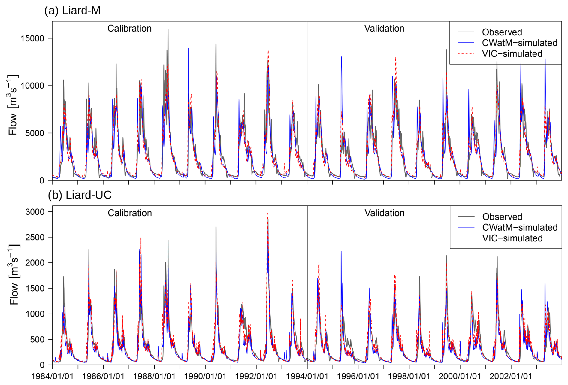
Figure 2 Observed vs. simulated discharge from CWatM and VIC models for calibration (1984–1994) and validation (1994–2004) periods for (a) Liard-M station and (b) Liard-UC station.

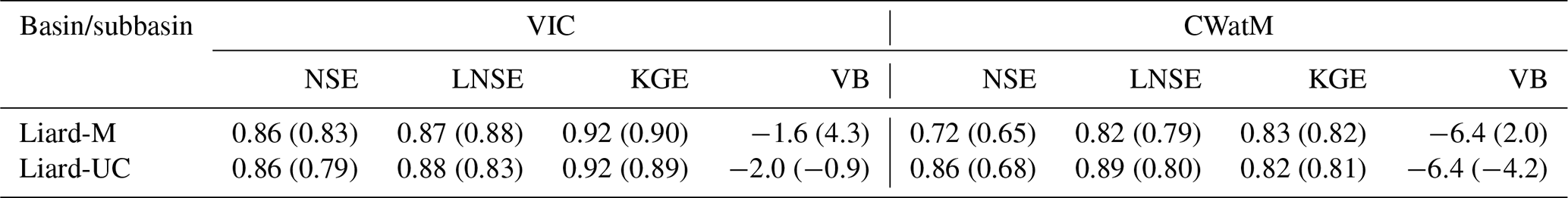
The comparison of the statistical GOF metrics of NSE, LNSE, KGE and VB reveals generally better performance for VIC compared to CWatM (Table 3). The two models are calibrated using different objective functions, which could potentially lead to some differences in the model performance. Furthermore, the performance of the selected models is influenced by model selection based on automatic calibration supplemented by the modeller's judgement. Specifically, for the Liard-UC station for the calibration period, the KGE performance for CWatM is inferior to that of VIC, although KGE was used as an objective function for the calibration for CWatM but not for VIC. In contrast, the NSE and LNSE performances of CWatM – which are used for the calibration of VIC but not for CWatM – are similar to that of VIC. Additionally, while VIC results are similar for the Liard-UC and Liard-M stations, CWatM performed better for Liard-UC than Liard-M. Several factors likely contribute to these differences. Firstly, the subdivision of the LRB into 28 subbasins allowed VIC to parameterize and calibrate to subbasin-specific conditions (6 parameters × 28 subbasins in total), and the use of calibrated upstream flows as inflows helped to better match the flows at the outlets of Liard-UC and Liard-M. In contrast, since CWatM was calibrated by lumping the large LRB into only two sets of parameters (10 parameters × 2 subbasins), it is not able to capture the subbasin-level heterogeneity. Additionally, the aforementioned differences in model structure, especially those related to frozen ground and groundwater, affect the runoff generation processes and subsequently model performance. Particularly, the frost index method in CWatM, which prevents infiltration through the top two soil layers under frozen soil condition, likely led to a higher proportion of surface runoff and earlier peak flows in CWatM compared to VIC, which allows infiltration through frozen soil using the coupled soil thermal and moisture flux representation (Cherkauer and Lettenmaier, 2003). Besides these model-related differences, both model results are also affected by uncertainties associated with input and calibration data. Specifically, the representativeness of the precipitation and temperature in the PNWNAmet dataset due to sparse station density at the high-latitude region (Werner et al., 2019), as well as limitations in observed discharge estimation during ice-covered and ice breakup events (Hamilton and Moore, 2012), can be major sources of uncertainty.

Table 3 Comparison of the goodness-of-fit (GOF) metrics for VIC and CWatM results. Summarized metrics include Nash–Sutcliffe coefficient of efficiency (NSE), NSE of log flows, Kling–Gupta coefficient (KGE) and percent volume bias (VB) for calibration (validation) 1984–1993 (1994–2003). NSE, LNSE and VB were used as objective functions for the calibration of VIC, and KGE was used as an objective function for the calibration of CWatM.

Further, the comparison of VIC- and CWatM-simulated snow water equivalent (SWE) with observations at three snow pillow sites with the highest number of observations generally shows a good replication of the seasonal dynamics by both models (Fig. S1 in the Supplement). Specifically, the seasonal SWE accumulation and ablation, as well as maximum SWE values, are reasonably well replicated by both models. The good model performance is also indicated by GOF values (Table S2). The SWE simulations from both models are also affected by uncertainties related to model structure and meteorological inputs, as discussed earlier. Additional sources of uncertainty include the mismatches between the observation station location and elevation with the model grid and elevation band, respectively, and measurement errors (e.g., SWE calculation from snow depth). Nevertheless, given the reasonable replication of the magnitude and dynamics of observed SWE and streamflow, as well as VIC-simulated values, the calibrated CWatM can be considered suitable for projecting future hydrologic responses.

4.2 Temperature and precipitation changes

Before evaluating projected future hydrologic responses from VIC and CWatM, we analyzed the MBCn downscaled temperature and precipitation from the GCM ensemble. As expected, the seasonal and annual temperature and precipitation over the LRB show progressive increases with the GWLs (Fig. 3). Furthermore, consistent with the projected higher warming over northern latitudes (Flato et al., 2019), the basin-scale seasonal and annual temperature increases are higher than global temperature increases, with median increases of +1.8, +2.6, +4.1 and +5.6 °C relative to the 1971–2000 period at +1.5 (or +1.0 global warming from 1971–2000), +2.0 (+1.5), +3.0 (+2.5) and +4.0 (+3.5) °C GWLs, respectively. Seasonally, higher temperature increases are projected for the colder months (October–November–December (OND) and January–February–March (JFM)) than warmer months (April–May–June (AMJ) and July–August–September (JAS)).

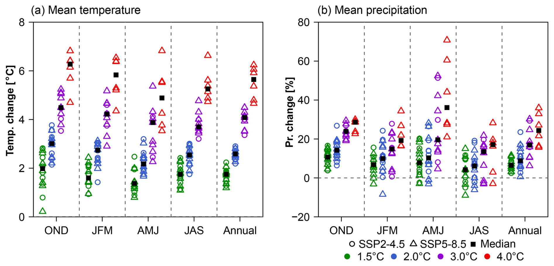
Figure 3 Mean annual and seasonal (a) temperature and (b) precipitation changes at 1.5 to 4.0 °C global warming levels (GWLs) relative to the 1971–2000 reference period. The projected changes for SSP2-4.5 and SSP5-8.5 scenarios are shown together in one column.

The projected annual precipitation in the LRB mostly shows progressive increases with GWLs, with median basin-scale annual increases of 6.5, 8.8, 16.9 and 24.3 % relative to the 1970–2000 reference period at 1.5, 2.0, 3.0 and 4.0 °C GWLs, respectively. Seasonally, projected precipitation for most GCMs shows increases, with a larger variability of change for AMJ and smaller variability for OND. The median seasonal precipitation increases are largest in OND, except for the larger increases in AMJ at 4.0 °C GWL. Overall, the enhanced temperature and precipitation increases for CMIP6 GCMs over the LRB are similar to CMIP5 GCMs assessed in our previous study (Shrestha et al., 2019).

4.3 Annual water balance change

We first compared VIC and CWatM simulations of annual water balance variables, consisting of precipitation, evapotranspiration (ET) and runoff, averaged over the entire LRB (Fig. 4). Additionally, we assessed maximum SWE (SWEmax), as it is related to all water balance variables. The results from the two models depict very similar changes, characterized by progressive increases in annual ET and runoff in response to increasing precipitation and temperature. SWEmax changes are minimal at the four GWLs for both models, suggesting that the projected winter precipitation increases offset the temperature-driven snowpack declines. The ranges of median percentage changes are generally similar, and models typically agree on the direction of median change, except for the small changes in SWEmax.

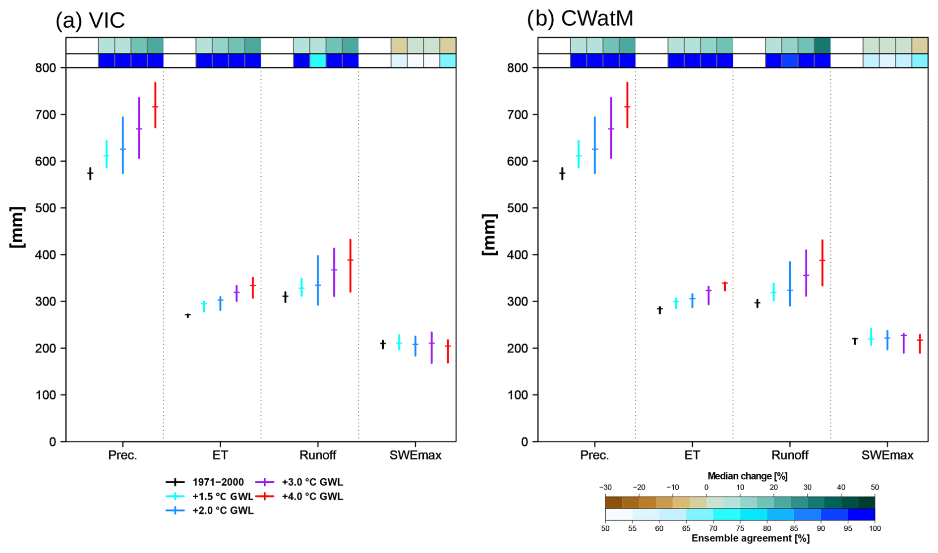
Figure 4 Historical (1971–2000) and projected annual water balance variables [mm] at 1.5 to 4.0 °C GWLs obtained from the GCM ensemble. The results show basin-averaged values for the entire Liard River basin, consisting of precipitation used as forcings, and (a) VIC and (b) CWatM-simulated evapotranspiration (ET), runoff and maximum snow water equivalent (SWEmax). Median change [%] at the four GWLs relative to 1971–2000, along with the agreement of ensemble members [%] with the direction of median change, is shown on the top of each panel.

The results are consistent when comparing the distribution of precipitation between ET and runoff. Specifically, for both models, the median ET $/$ precipitation ratios range between 0.45 and 0.48, while the runoff $/$ precipitation ratios range between 0.52 and 0.55, with generally decreasing ET $/$ precipitation ratios and increasing runoff $/$ precipitation ratios at higher GWLs. Furthermore, the median SWEmax $/$ October–March precipitation ratios, with a ratio > 0.5 used to characterize the hydrologic regime of a basin as snow-dominated (Elsner et al., 2010), decline successively from 0.84 to 0.65 with higher GWLs for both models. Overall, the projected annual water balance changes from CWatM are consistent those from VIC.

4.4 Monthly SWE changes

Changes in basin-averaged monthly SWE values from the two models at different GWLs are also generally consistent (Fig. 5). Both models show slightly higher SWE accumulation in the colder upstream Liard-UC subbasin than the entire Liard-M basin. Furthermore, monthly SWE values successively decline with higher GWLs during October and November, while the changes from December to March are relatively smaller. Monthly SWE values also decline successively with higher GWLs in April and May, with CWatM showing more rapid declines, particularly for the Liard-UC subbasin. However, the differences are marginal, the direction of median changes is generally consistent between VIC and CWatM for both Liard-M and Liard-UC. Additionally, the model ensembles show higher agreement with the direction of median change in the months with larger snowpack loss (October, November, May and June) and lower agreement in the months with smaller snowpack change (January to March). The generally consistent monthly SWE and SWEmax results (Figs. 4 and 5) suggest that the differences in snowmelt algorithms in the two models (VIC: full energy balance; CWatM: radiation-restricted degree-day) have a minor effect on the magnitude and timing of snowmelt at the basin-scale and monthly time periods. However, these results may have been influenced by the necessity to calculate all energy fluxes from the same air temperature, precipitation and wind speed datasets for both models using MTCLIM.

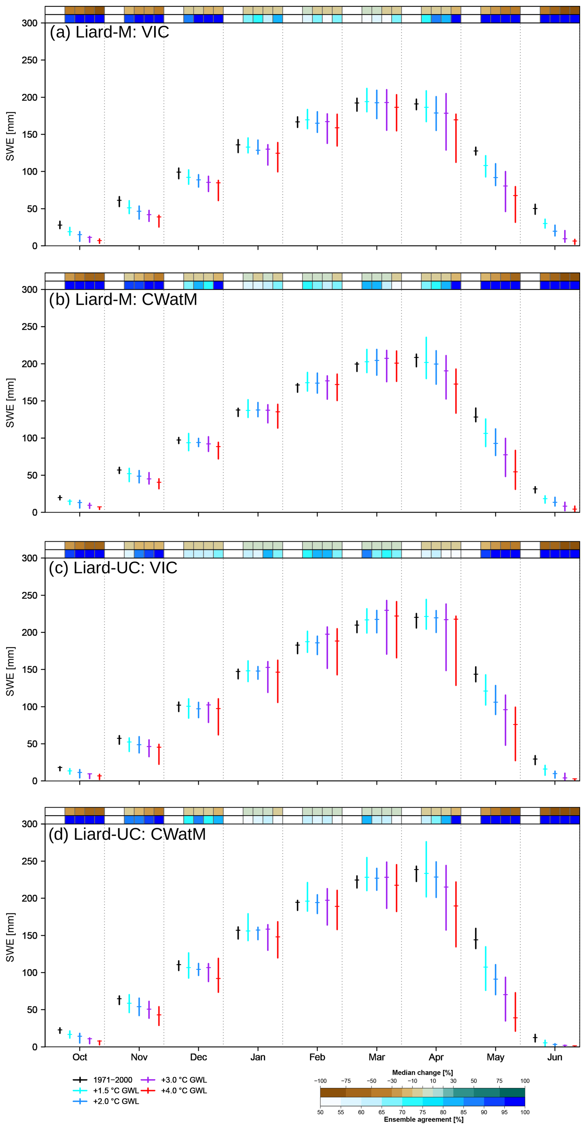
Figure 5 Historical (1971–2000) and projected monthly SWE [mm] at 1.5 to 4.0 °C GWLs obtained from the GCM ensemble. All SWE results are simulated, basin-averaged values from model simulations, consisting of (a) VIC for Liard-M station, (b) CWatM for Liard-M station, (c) VIC for Liard-UC station and (d) CWatM for Liard-UC station. Median change [%] at four GWLs relative to 1971–2000, along with the agreement of the ensemble members [%] with the direction of median change, is shown on the top of each panel. July to September months are not shown because SWE values are very small.

4.5 Monthly and maximum flow changes

A key challenge in modelling hydrologic change is accurately simulating different flow components, such as monthly mean flows and maximum and minimum flows. A comparison of the VIC- and CWatM-simulated monthly flows from the ensemble with observations over the period 1971–2000 shows that both models have difficulty in replicating observed flows in some months, as indicated by the range of simulated flows from the ensemble not covering the observed flow values (Fig. 6). Based on this criterion, both model simulations depict larger discrepancies for the Liard-M station and relatively smaller discrepancies for the upstream Liard-UC station. In the case of maximum flow, the ensemble range generally covers the observed flow values, with similar performance for VIC and CWatM simulations (Fig. 7). For maximum flow timings, the discrepancies between observations and simulated median values are of the order of 3 to 8 d, with the ensemble from VIC not covering the observed flow values for either stations. Such mixed model performance in replicating different components of streamflow hydrographs is partly related to model uncertainties discussed in Sect. 4.1. Similar discrepancies in reproducing streamflow components by different hydrologic models have also been reported in previous studies (e.g., Shrestha et al., 2014, 2019; Vigiak et al., 2018; Visser-Quinn et al., 2019). Given this challenge, it is common practice to assess future hydrologic changes as a relative change between simulated historical and future flows (e.g., Schnorbus et al., 2014; Eum et al., 2016; Byun et al., 2019; Shrestha et al., 2019), and the same approach is used in this study for benchmarking future hydrologic change.

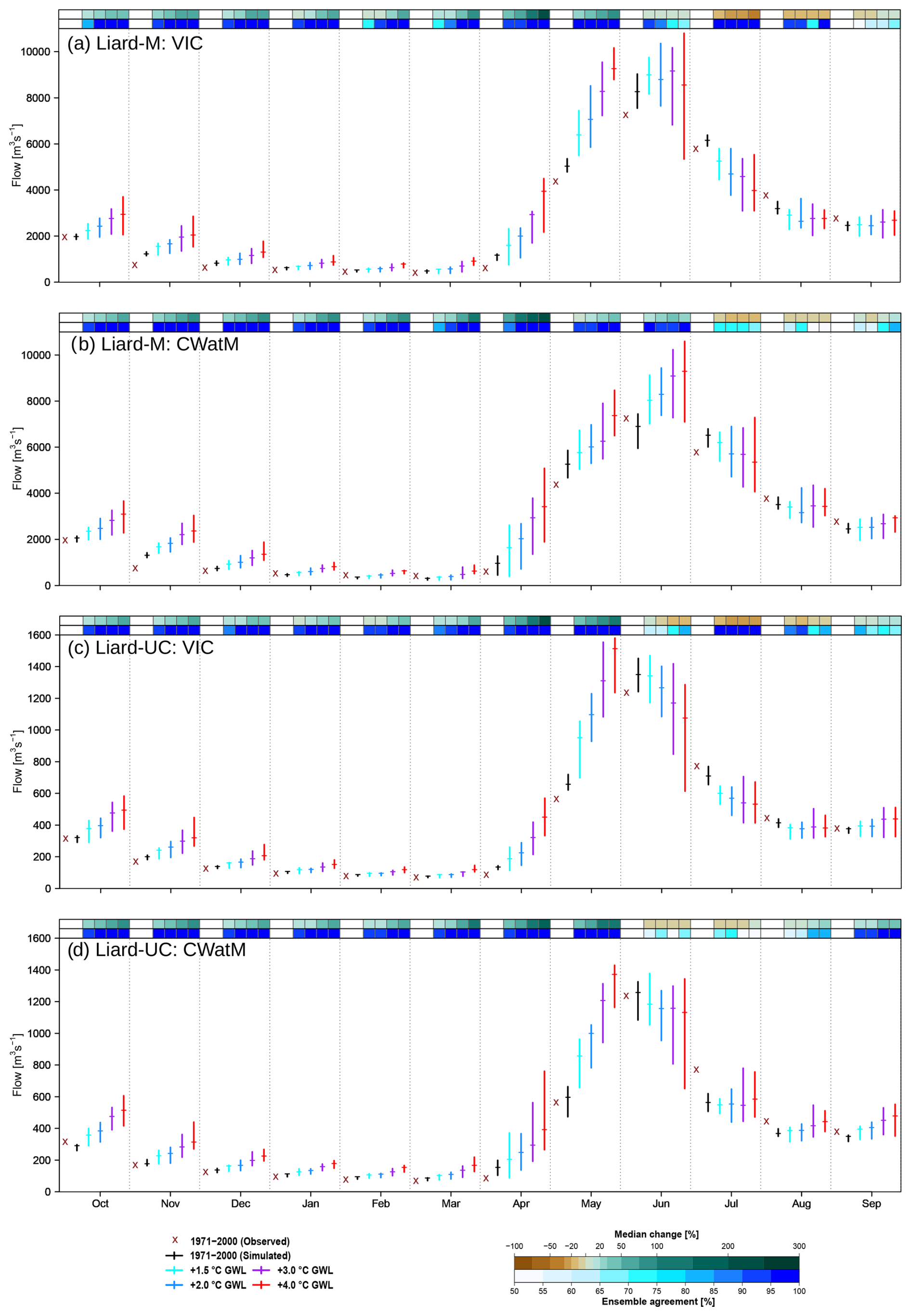
Figure 6 Historical (1971–2000) and projected monthly flow at 1.5 to 4.0 °C GWLs obtained from the GCM ensemble, consisting of (a) VIC for Liard-M station, (b) CWatM for Liard-M station, (c) VIC for Liard-UC station and (d) CWatM for Liard-UC station. Median change [%] at four GWLs relative to 1971–2000, along with the agreement of the ensemble members [%] with the direction of median change, is shown on the top of each panel.

Simulated mean monthly flow (Q_mean) projections from the two models display consistent patterns, with progressive increases in cold-season (October–March) flows with higher GWLs for both Liard-M and Liard-UC stations (Fig. 6). Furthermore, both models project generally increased Q_mean with higher GWLs in April and May, following the declining SWE patterns for these 2 months (Fig. 5). The direction of projected Q_mean change in June differs between the two stations but is consistent between VIC and CWatM, with a declining pattern at higher GWLs for the upstream Liard-UC station and an increasing pattern for the downstream Liard-M station. The larger uncertainties in projected AMJ precipitation at 3.0 and 4.0 °C GWLs (Fig. 3) likely contributed to larger spreads of the projected flow responses during these months and GWLs. July and August Q_mean projections from the two models show some differences, with CWatM projections showing smaller declines for Liard-M and smaller decreases or increases for Liard-UC, compared to VIC, which shows larger declines for both stations. September Q_mean responses are consistent between the two models, with progressive increases in flows at higher GWLs. These similarities and differences in responses between the two models are also reflected by the median changes and model ensemble agreements. Specifically, both models show progressive increases in median values and high model agreements among ensemble members between October and May. For June to August, the median changes are less consistent, and direction of changes shows lower agreement.

These differences in VIC and CWatM projections arise from the combined effect of several factors related to process representation and parameterization. As discussed, the differences in the treatment of frozen soil processes in the two models affect infiltration and runoff pathways, with a higher proportion of surface runoff generation in CWatM than in VIC (Fig. S2), influencing early-summer (June) Q_mean. On the other hand, the presence of groundwater storage in CWatM, which stores percolated water and releases it as baseflow using a linear reservoir approach (Burek et al., 2020), delays the baseflow response and results in a higher late-summer (July and August) Q_mean from CWatM than from VIC, which uses a nonlinear baseflow function to release water stored in the bottom layer. Other factors that contribute to these differences include the routing method and parameterization, which influence runoff transport through the watershed and the timing and magnitude of flow delivered to the outlet, and the differences in watershed subdivision and model calibration. However, despite the inferior calibration performance for the downstream Liard-M station (Table 3), CWatM projection results for this station are not substantially different from VIC results. This suggests that the uncertainties in projected responses due to lumped parameters and calibration may be relatively small.

Projected changes in maximum flows (Q_max) and their timing are generally consistent between the two models in terms of the direction of change and are seen to be dependent on GWLs, with progressively higher Q_max values and earlier Q_max timing with higher GWLs for both Liard-M and Liard-UC (Fig. 7). However, while the median Q_max values and timing are similar between the two models for Liard-UC, Liard-M Q_max values are generally smaller, and Q_max timing occurs earlier for CWatM, compared to corresponding projections from VIC.

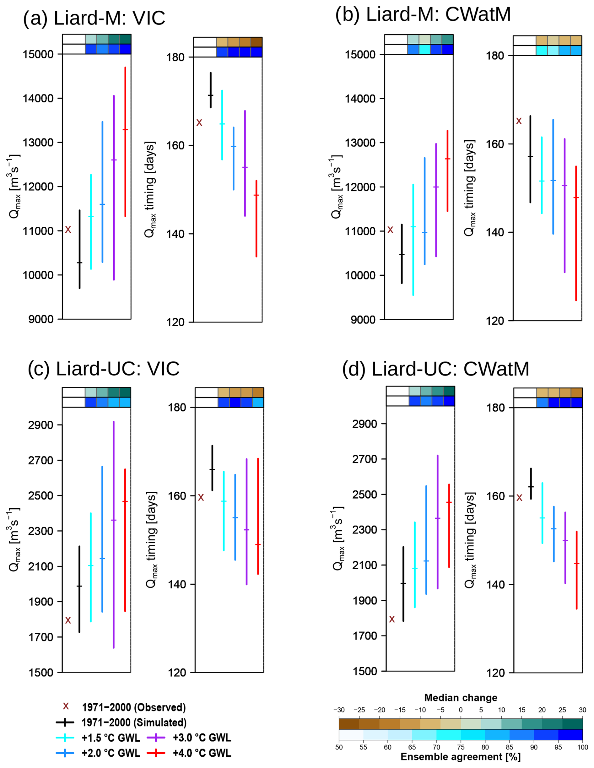
Figure 7 Historical (1971–2000) and projected annual maximum flows and their timings at 1.5 to 4.0 °C GWLs obtained from the GCM ensemble. Median change [% or d] at four GWLs relative to 1971–2000, along with the agreement of ensemble members [%] with the direction of median change, is shown on the top of each figure panel.

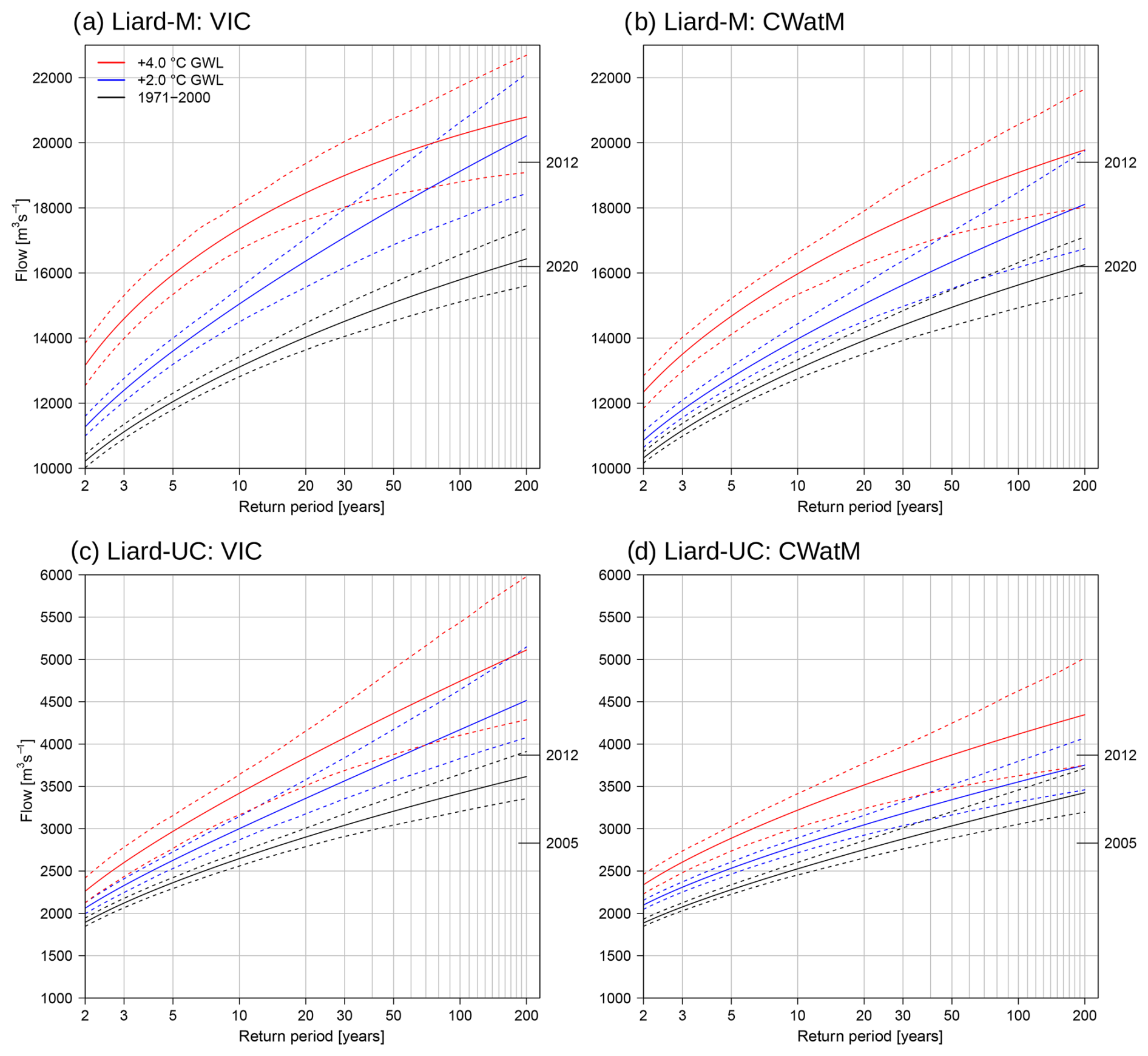
Figure 8 Flood frequency plots of annual maximum flows obtained from the model simulations driven by the GCM ensembles: (a) VIC for Liard-M station, (b) CWatM for Liard-M station, (c) VIC for Liard-UC station and (d) CWatM for Liard-UC station. The results are shown for the historical period (1971–2000) and 2.0 and 4.0 °C GWLs. Dashed lines show the 95 % confidence intervals. The years on the right axes of each plot indicate the two highest-recorded historical flood events.

The 2- to 200-year flood frequency curves show progressively higher flow values at a given return period at 2.0 and 4.0 °C GWLs compared to the 1971–2000 reference period for both models and stations (Fig. 8). An alternative interpretation of these nonstationary changes is that the return periods associated with specific magnitudes of flow decrease with higher GWLs. Increasing spreads of the 95 % confidence intervals from 2- to 200-year return periods can also be seen from both models and stations. Interestingly, the flood frequency curve for Liard-M at 3.0 °C GWL (Fig. S3) covers a higher range than at 4.0 °C for both models, especially at higher return periods (> 40-year periods for VIC and > 80-year periods for CWatM). Although such patterns are not present for the Liard-UC station, the results for 4.0 °C GWL are affected by a smaller sample size (6×20 values) compared to 3.0 °C (12×20 values), given that 6 and 12 out of 16 ensemble members reach 3.0 and 4.0 °C GWLs, respectively.

Additionally, while the flood frequency curves are similar for the 1971–2000 reference period for the two models, the curves tend to diverge at higher GWLs and return periods, and the magnitudes of extreme flows at a specific return period are considerably lower for CWatM than VIC (Fig. 8). For Liard-UC, it is notable that extreme flow values from the flood frequency curves are substantially lower for CWatM than corresponding values for VIC, although the median values from the two models are close to each other (Fig. 7). The divergence in responses arises from the differences in distribution of the entire ensemble, with the higher upper limit of VIC projections contributing to higher values in the flood frequency curves for both stations. As such, while the largest recorded 2012 flood events are within the range of the flood frequency curve at 1.5 °C GWL for VIC for both stations, they are only covered at 3.0 or 4.0 °C GWL for CWatM (Figs. 8 and S3).

As in the case of Q_mean, the magnitudes and timing of Q_max are affected by structural differences in the two models, particularly runoff pathways. Specifically, the earlier Q_max timing in CWatM than VIC can be linked to the higher fraction of quicker-flowing surface runoff in the former (Fig. S2), resulting from the frost index method that prevents soil water movement through the frozen soil. The higher Q_max from VIC compared to CWatM can be linked to the lack of groundwater storage in the former, which causes baseflow to increase rapidly using a nonlinear function when soil moisture exceeds a certain threshold and gets added to the total runoff (Fig. S2). Hence, the lack of groundwater storage in VIC likely causes an overestimation of annual maximum flows, and the lack of soil water movement through the frozen soil in CWatM likely causes an overestimation of the surface runoff contribution to the annual maximum flow and earlier annual maximum flows. However, notwithstanding these differences, key climate change signals of earlier and higher maximum flows, nonstationary increases in the magnitudes of extreme flows, are consistent between the two models.

5 Summary and conclusions

Our study contributes important insights into the robustness of future hydrologic projections from a large-scale hydrologic model (LHM) in comparison to a watershed hydrologic model (WHM). As suggested by Beven (2023), we designed a fit-for-purpose benchmarking study to compare future hydrologic projections from a state-of-the-art CWatM simulation with the widely used VIC model for the Liard River basin in subarctic Canada, with CWatM setup as an LHM with two subbasins and VIC setup as a WHM with 28 subbasins. We used a consistent set of downscaled CMIP6 climate forcings to drive the two models. Since the assessment focuses on a northern basin and the structure of the two models differs in terms of representation of cold-climate snowmelt and frozen soil processes, our study provides a good case for evaluating the effects of model structural uncertainties on historical and future projections.

Our evaluation revealed generally consistent patterns of projected hydrologic responses from the two models in terms of annual water balance and monthly distribution of SWE and flow. Key hydrologic change signals of increasing annual evapotranspiration and runoff with higher global warming levels are projected by both models. CWatM is also able to replicate the prominent snowpack change signals from VIC, particularly the successive declines in late-spring SWE with higher GWLs. Likewise, CWatM simulates increasing winter and spring flows with higher GWLs, consistent with the VIC model simulation. The direction of maximum flow and timing changes from CWatM are generally in agreement with VIC, characterized by increasing and earlier flows with higher GWLs. However, the magnitude of annual maximum flows diverges between the two models, with CWatM generally producing lower magnitudes and earlier timing compared to corresponding VIC projections. These differences in the annual maximum flows are also reflected in the extreme value analysis, with CWatM projecting considerably smaller extreme flood events than VIC at all GWLs, especially for longer return periods.

The similarities and differences between the two model simulations lead to a subsequent question about the robustness of the projected changes. Overall, the consistency of the projected changes from the two models suggests that a calibrated LHM can provide robust projections of future hydrologic responses at annual and monthly timescales. The direction of SWE and flow changes obtained from both models are also consistent with the previous study based on CMIP5 GCM-driven VIC model simulations (Shrestha et al., 2019). Furthermore, generally consistent results from two models for upstream and downstream subbasins increase the confidence in projections. However, given that this study is focused on single cold-region river basin, broader generalization of the results to other regions is not recommended. Additionally, our results are specific to the calibrated CWatM LHM and not representative of the capabilities of other LHMs or GHMs.

An important consideration in this study is the representation of cold-climate processes of snow ablation and melt, as well as frozen soil. In this respect, CWatM produced very similar monthly and annual maximum SWE values when compared to VIC, despite having a simplified radiation-restricted snowmelt module versus the full energy balance in VIC. However, these results may have been influenced by the necessity to calculate all energy fluxes based on the same air temperature, precipitation and wind speed datasets for both models using MTCLIM. Differences in the representation of frozen soil processes, however, led to differences in surface and subsurface flow pathways. Specifically, the simplified frost index approach (Molnau and Bissell, 1983) in CWatM, which prevents soil water movement through the frozen soil, results in a higher fraction of surface runoff than VIC, which includes a coupled soil thermal and moisture fluxes approach, with soil water movement under frozen conditions dependent on ice content (Cherkauer and Lettenmaier, 1999, 2003). These differences in flow pathways seem to have affected late-summer monthly flows and annual maximum flows, with a larger fraction of surface runoff in CWatM likely resulting in earlier annual maximum flows. Additionally, the lack of groundwater storage in VIC likely led to a more rapid baseflow response and consequently an overestimation of annual maximum flow and amplified extreme values. In contrast, the groundwater storage in CWatM, albeit a simplified linear reservoir approach, likely caused a delayed baseflow response and smaller maximum flows, as well as a smaller reduction or no change in summer flows. Regarding other factors, such as the subdivision of the watershed into subbasins and model calibration, given that the projected results are not substantially different for the downstream Liard-M station despite lumped parameter sets and inferior calibration performance, their effects seem small.

Overall, the CWatM setup for the Liard River basin is generally able to replicate the projected hydrologic responses from VIC. The results are very consistent for directions of change and most magnitudes of change, except maximum flows and summer flows. Hydrologic model structural uncertainties, specifically the representation of frozen soil and groundwater processes, provide an explanation for the differences in the annual maximum flows and summer flows. Given such uncertainties, an important consideration is the robustness of model structure in simulating hydrologic metrics of interest for climate change impacts research (Ekström et al., 2018; Shrestha et al., 2016). Based on the findings of this study, an implementation of groundwater storage in VIC could potentially lead to a better representation of runoff pathways and timing, as well as improvement in the streamflow simulation. On the other hand, an improved frozen soil method in CWatM could potentially lead to a better representation of groundwater storage and improvement in the surface runoff and baseflow partitioning, with consequently improved streamflow response at the basin outlet. Such enhancements have a potential to reduce the uncertainties in future hydrologic projections. Hence, our results provide an important basis for improving not only the LHMs but also the WHMs.