Flexible forecast value metric suitable for a wide range of decisions: application using probabilistic subseasonal streamflow forecasts

Streamflow forecasts have the potential to improve water resource decision-making, but their economic value has not been widely evaluated, since current forecast value methods have critical limitations. The ubiquitous measure for forecast value, the relative economic value (REV) metric, is limited to binary decisions, the cost–loss economic model, and risk-neutral decision-makers (users). Expected utility theory can flexibly model more real-world decisions, but its application in forecasting has been limited and the findings are difficult to compare with those from REV. In this study, a new metric for evaluating forecast value, relative utility value (RUV), is developed using expected utility theory. RUV has the same interpretation as REV, which enables a systematic comparison of results, but RUV is more flexible and better represents real-world decisions because more aspects of the decision context are user-defined. In addition, when specific assumptions are imposed, it is shown that REV and RUV are equivalent, hence REV can be considered a special case of the more general RUV. The key differences and similarities between REV and RUV are highlighted, with a set of experiments performed to explore the sensitivity of RUV to different decision contexts, such as different decision types (binary, multi-categorical, and continuous-flow decisions), various levels of user risk aversion, and varying the relative expense of mitigation. These experiments use an illustrative case study of probabilistic subseasonal streamflow forecasts (with lead times up to 30 d) in a catchment in the southern Murray–Darling Basin of Australia. The key outcomes of the experiments are (i) choice of decision type has an impact on forecast value, hence it is critically important to match the decision type with the real-world decision; (ii) forecasts are typically more valuable for risk averse users, but the impact varies depending on the decision context; and (iii) risk aversion impact is mediated by how large the potential damages are for a given decision. All outcomes were found to critically depend on the relative expense of mitigation (i.e. the cost of action to mitigate damages relative to the magnitude of damages). In particular, for users with relatively high expense of mitigation, using an unrealistic binary decision to approximate a multi-categorical or continuous-flow decision gives a misleading measure of forecast value for forecasts longer than 1 week lead time. These findings highlight the importance of the flexibility of RUV, which enable evaluation of forecast value to be tailored to specific decisions/users and hence better capture real-world decision-making. RUV complements forecast verification and enables assessment of forecast systems through the lens of user impact.

1 Introduction

Effective water resource management is critically important to human welfare, thriving environmental ecosystems, agricultural productivity, power generation, town supply, and economic growth (United Nations, 2011; UNESCO, 2012). The management and equitable distribution of water to competing stakeholders is challenging due to long-term decreasing trends in available surface water (Zhang et al., 2016), increasing high-intensity storm events (Tabari, 2020), river basins over-allocated to irrigated agriculture (Grafton and Wheeler, 2018), and deteriorated ecosystems dependent on river systems (Cantonati et al., 2020). Environmental decision-making depends largely on the current and anticipated hydrometeorological conditions and is frequently informed by streamflow forecasts. Many decisions, such as reservoir operations and early flood warnings, benefit from forecasts at a subseasonal time horizon (2–8 week lead times) because of long river travel times, operational constraints, and logistical overheads (White et al., 2015; Monhart et al., 2019). Previous studies have used forecast verification techniques to demonstrate that subseasonal streamflow forecasts are becoming more skilful at longer lead times with reliable estimates of uncertainty (Schmitt Quedi and Mainardi Fan, 2020; McInerney et al., 2020). However, it is not clear whether forecasts should be used to inform water-sensitive decisions once economic and other factors are considered, thus posing the key question, “do the forecasts provide economic value for decisions-makers?”. These factors are typically not considered when evaluating the performance of forecasts, largely due to the limitations of available forecast value methods. This study addresses this gap by developing a new forecast value method that is applicable for a wide range of water-sensitive decisions, such as storage release management and environmental watering.

Forecast verification is the comparison of a set of forecasts spanning a historical period to the observed record using statistical performance metrics. The hydrological forecasting community uses numerous statistical metrics to summarise the performance of ensemble forecasts, including the continuous rank probability score (CRPS) for accuracy and metrics based on the probability integral transform for statistical reliability (e.g. Cloke and Pappenberger, 2009; McInerney et al., 2017; Woldemeskel et al., 2018; Bennett et al., 2021). Forecast verification is necessary but insufficient for users to confidently adopt forecasts into their operational and strategic decision-making processes. For example, it does not consider the broader context for which a decision is made, the economic trade-offs, and different decision types. Forecast value measures the improvements, in an economic sense, that can be achieved by using one source of forecast information relative to another. It explicitly considers the broader decision context, with economics being one of the most tractable aspects to analyse. When using forecast verification as a proxy for forecast value, we are implicitly assuming that better forecast performance (according to our verification metrics) implies more value. However, additional forecast performance is not necessarily a good predictor of additional benefit to a user (Murphy, 1993; Roebber and Bosart, 1996; Marzban, 2012). Exploring the relationship between forecast performance and value over a range of use cases and lead times is an active area of research, particularly for inflows into hydropower reservoirs (Turner et al., 2017; Anghileri et al., 2019; Peñuela et al., 2020; Cassagnole et al., 2021) and early-warning decision making for extreme events (Bischiniotis et al., 2019; Lopez et al., 2020; Lala et al., 2021).

Streamflow forecasts can improve the outcomes of a range of decisions, including binary, multi-categorical, and continuous-flow decision types. For example, water level exceeding the height of a levee is a binary decision, and emergency response decisions in relation to a minor, moderate, and major flood classification is a familiar multi-categorical decision. A mitigation decision based on continuous flow is the limiting case of a very large number of flow classes – for example, adjusting dam releases to match storage inflow during flood operations. While decisions involving more flow classes are an essential feature of many real-world decisions, a binary decision has traditionally been used as the prototypical model of decision-making in decision-theoretic literature (Katz and Murphy, 1997). The most frequently used forecast value method in hydrology and meteorology is relative economic value (REV), which is unable to handle a wide range of decision types. Substantial research in the field of meteorology has explored the value of temperature, wind, and rainfall forecasts for user decisions using REV (e.g. Richardson, 2000; Wilks, 2001; Mylne, 2002; Palmer, 2002; Zhu et al., 2002; Foley and Loveday, 2020; Dorrington et al., 2020). There is an ongoing interest in hydrology to quantify the value of forecasts for decision-making using REV (e.g. Laio and Tamea, 2007; Roulin, 2007; Abaza et al., 2013; Thiboult et al., 2017; Verkade et al., 2017; Portele et al., 2021), although there have not been applications with subseasonal streamflow forecasts. REV is convenient in its tractability but has strong assumptions about the decision type, economic model, and user behaviour that neglect important aspects of decision-making and have implications on the conclusions reached (Tversky and Kahneman, 1992; Katz and Murphy, 1997; Matte et al., 2017; An-Vo et al., 2019).

REV is only suitable to assess forecast value for risk-neutral users making binary decisions using a cost–loss economic model and event frequency reference baseline (Thompson, 1952; Murphy, 1977). This limited setup is an excellent prototypical decision model, which is useful to understand the salient features of forecast value, but may give misleading results when used to model real-world decisions. For example, flood warnings are a practically important multi-categorical decision, typically classified into either minor, moderate, or major flood impact levels, whereas REV only handles binary decisions. Likewise, adjusting the release of water from a storage is best informed by continuous-flow forecasts and may require a more complex economic model than the cost–loss economic model assumed by REV.

REV is also unable to consider the impact of risk-averse users. A user is said to be risk averse if they prefer an option with a more certain outcome, even if it may on average lead to a less economically beneficial outcome (Werner, 2008). For example, a water authority deciding to announce a large water allocation event, or an irrigator placing an order, exhibit risk aversion if they prefer a forecast outcome that is almost certain to occur rather than one that is uncertain but potentially more beneficial.

The field of decision theory explores how agents make decisions with uncertain information, and has produced a number of innovations such as expected utility theory (Neumann, 1944; Mas-Colell, 1995). Expected utility theory is flexible enough to model different decision types, economic models, and risk aversion, but there is limited understanding of the relationship and differences between it and REV. It proposes that when faced with a choice, a rational person will select the option leading to an outcome that maximises their utility; an ordinal measure based on the ranking of outcomes. Different people may rank outcomes differently because of their specific preferences, such as risk aversion. While expected utility theory is widely used in economics, public policy, and financial management, it has had a very limited application in hydrology and associated fields. Recently, Matte et al. (2017) applied expected utility theory in a flood damage application to assess the impact of increasing intangible losses and risk aversion on the value of raw probabilistic streamflow forecasts for a single multi-categorical decision type with 12 flow classes. This study demonstrated some benefits of forecast value, but was case-study-specific, limited to a single multi-categorical decision, and used metrics that are somewhat unfamiliar to the verification community. The results were not presented on a traditional value diagram, and therefore no comparison to REV could be made. We are unaware of any literature that attempts to align REV with forecast value from expected utility theory or present the results on a value diagram. There is no method available to the verification community to flexibly evaluate the value of probabilistic forecasts for different decision types, economic models, or user characteristics (Cloke and Pappenberger, 2009; Soares et al., 2018).

Probabilistic forecasts of continuous hydrometeorological variables lead to improved forecast performance in many cases and are operationally delivered by all major forecast producers, but users are still learning the most effective way to use them (Duan et al., 2019; Carr et al., 2021). A common approach for decision-making with a probabilistic forecast is to convert it to a deterministic forecast using a fixed critical probability threshold (Fundel et al., 2019; Wu et al., 2020). This approach is known to lead to sub-optimal forecast value in some situations through studies using REV (Richardson, 2000; Wilks, 2001; Zhu et al., 2002; Roulin, 2007). Matte et al. (2017) quantified forecast value with an alternative decision-making approach which uses the whole forecast distribution to decide on an ideal action at each forecast update. It is not clear that this alternative approach leads to better decision outcomes and we are unaware of any literature comparing them.

The study aims are as follows:

1. develop a methodology to systematically compare two forecast value techniques; REV and a method based on expected utility theory;

2. demonstrate the key differences and similarities between the approaches for different decision types and levels of risk aversion using subseasonal streamflow forecasts in the Murray–Darling Basin.

In Sect. 2, the theoretical background of REV and an expected utility theory approach for forecast value are introduced. Section 3 proposes a new metric (relative utility value) based on expected utility theory and details its equivalence to REV when a set of assumptions are imposed. Section 4 introduces an illustrative case study using subseasonal forecasts and a series of experiments to explore the sensitivity of forecast value to different aspects of decision context. Results of the case study are presented in Sect. 5 and discussed in Sect. 6, including implications for forecast users and producers. Conclusions are drawn in Sect. 7.

2 Theoretical background

The background theory introduced here focuses on two methods to quantify the value of forecasts, namely REV and an approach using expected utility theory introduced by Matte et al. (2017).

2.1 Relative economic value

REV is a frequently used and excellent method to quantify the value of forecasts for cost–loss binary decision problems (Richardson, 2000; Wilks, 2001; Zhu et al., 2002). Cost–loss is a well-studied economic model where some of the loss due to a future event can be avoided by deciding to pay for an action which will mitigate the loss (Thompson, 1952; Murphy, 1977; Katz and Murphy, 1997). Many real-world decisions, such as insurance, can be simplified and framed in this way as a binary categorical decision. The method assumes that any real-world decision it is applied to can be framed in this way.

2.1.1 REV with deterministic forecasts

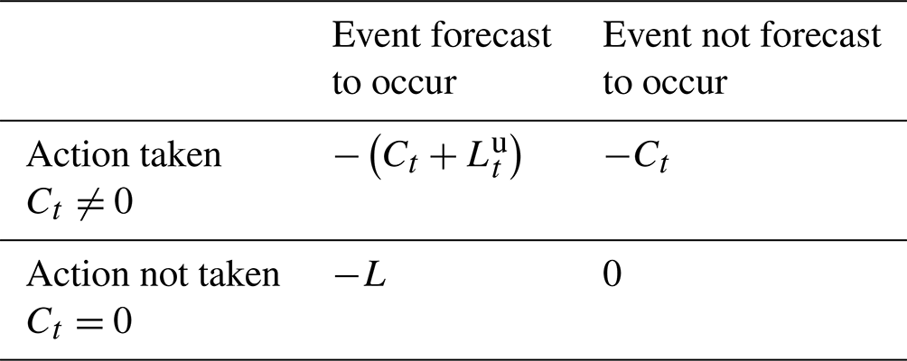
Whether a user is expected to benefit in the long run from the use of a forecast system (or an alternative) can be assessed using a 2×2 contingency table. Table 1 includes the hit rate h, miss rate m, false alarm rate f, and correct rejection rate (quiets) q from a long run historical simulation, along with the net expense from each combination of action and occurrence, where C is the cost of an action to mitigate the loss L. However, only a portion L_a of the total loss can be avoided with the remainder L_u being unavoidable. A derivation of Eq. (2) is provided in Sect. S1 of the Supplement.

Table 1 Contingency table for the cost–loss decision problem with expenses from each possible combination of action and occurrence. Here, C is the cost of the mitigating action, L_u is the unavoidable portion of loss L from the event occurring, and L_a is avoidable portion of loss from the action.

The expected long run expense E of each combination of action and occurrence depends on the rate that combination occurred over some historical period, and these rates will be different depending on which forecast information is used. The REV metric is constructed by comparing the relative difference in the total net expenses for decisions made using forecast, perfect, and climatological baseline information,

$$\begin{array}{}\text{(1)}& \mathrm{REV}={\displaystyle \frac{E_{\mathrm{climate}}-E_{\mathrm{forecast}}}{E_{\mathrm{climate}}-E_{\mathrm{perfect}}}},\end{array}$$

where $-\mathrm{\infty }<\mathrm{REV}\le \mathrm{1}$ and each expense term is the summation of the contingency table elements each weighted by the rate of occurrence. Equation (1) is equivalent to the following standard analytical equation for REV (Zhu et al., 2002) when the long run average expenses from Table 1 are considered,

$$\begin{array}{}\text{(2)}& \mathrm{REV}={\displaystyle \frac{\min \left(\stackrel{\mathrm{‾}}{o},\mathit{\alpha }\right)-(h+f)\mathit{\alpha }-m}{\min \left(\stackrel{\mathrm{‾}}{o},\mathit{\alpha }\right)-\stackrel{\mathrm{‾}}{o}\mathit{\alpha }}},\end{array}$$

where $\stackrel{\mathrm{‾}}{o}$ is the frequency of the binary decision event and the parameter α is known as the cost–loss ratio.

$$\begin{array}{}\text{(3)}& \mathit{\alpha }={\displaystyle \frac{C}{L_{\mathrm{a}}}}.\end{array}$$

Equation (2) is typically applied over a range of αvalues and this set of REV results is plotted on a value diagram. This diagram provides a visualisation of how forecast value varies for users with different levels of costs required to mitigate a loss, and by extension mitigation of the underlying damages. An alternative interpretation of α, which we refer to as relative expense of mitigation (see Table 2), is the relative expense (i.e. cost) a user experiences to take action and mitigate (i.e. avoid) their exposure to damages (i.e. loss). It is a “relative” expense of mitigation because the expense magnitude (i.e. cost) is relative to the magnitude of the damages (i.e. loss). This interpretation is used in this study since it is more generalisable across different forecast value methods. Users with smaller cost–loss ratio have a relatively lower expense of mitigation due to their ability to leverage a lower amount of spending (small cost) to avoid larger future damages (large loss). Conversely, users with a large cost–loss ratio have relatively high expense of mitigation, as they require a higher amount of spending to avoid future damages. For the same event, the relative expense of mitigation will vary for different users and decision types. This relative expense of mitigation interpretation of α should not be confused with the expected long run expense E used in the derivation Eq. (2).

Table 2 Comparison of REV and RUV forecast value methods for defining decisions and user characteristics.

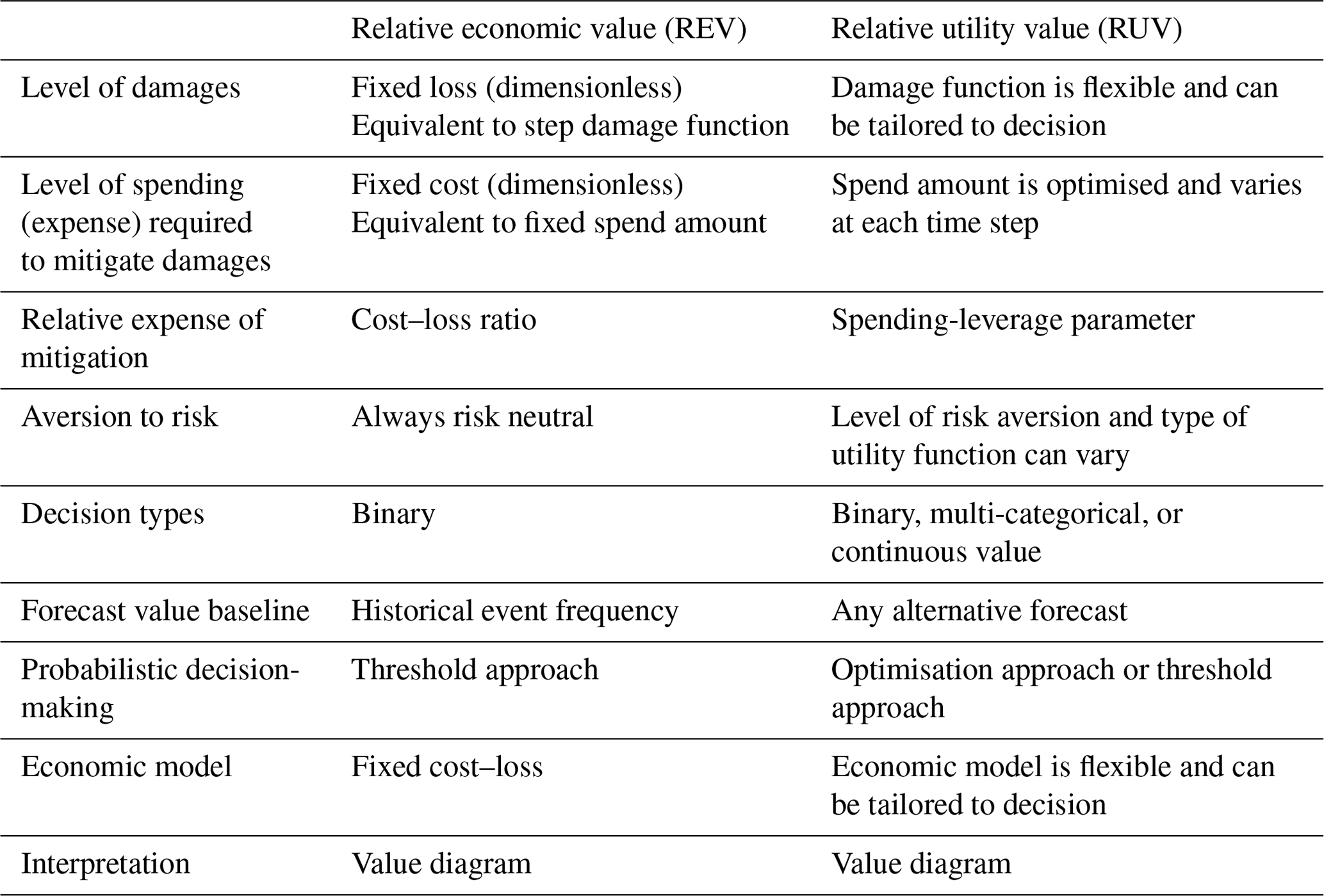
Figure 1 presents an illustrative value diagram as an aid to describe its interpretation (Richardson, 2000). The non-dimensional cost–loss ratio α is shown on the x axis and can be interpreted as a continuum of different decision-makers using the forecasts, with increasingly more expensive mitigation. A value of α=1 corresponds to maximum relative expense of mitigation; if losses are USD 100 000, then the amount to spend on a mitigating action is also USD 100 000. A value of α=0.1 indicates that only USD 10 000 would be needed to mitigate the loss. The y axis shows forecast value according to REV and has a similar interpretation to any skill score-based metric. A value of REV=1 indicates that decisions made using forecast information successfully mitigated the same level of losses (over the historical period) as decisions made using perfect information (streamflow observations). A value of REV=0 indicates the decisions were only as good as those made using reference baseline. A negative value indicates the decisions were worse than the reference. For example, a value of REV=0.7 at some value of α indicates that decisions made using forecasts led to a 70 % improvement in net expense relative to decisions made using the reference baseline, a similar interpretation to skill scores (Wilks, 1995).

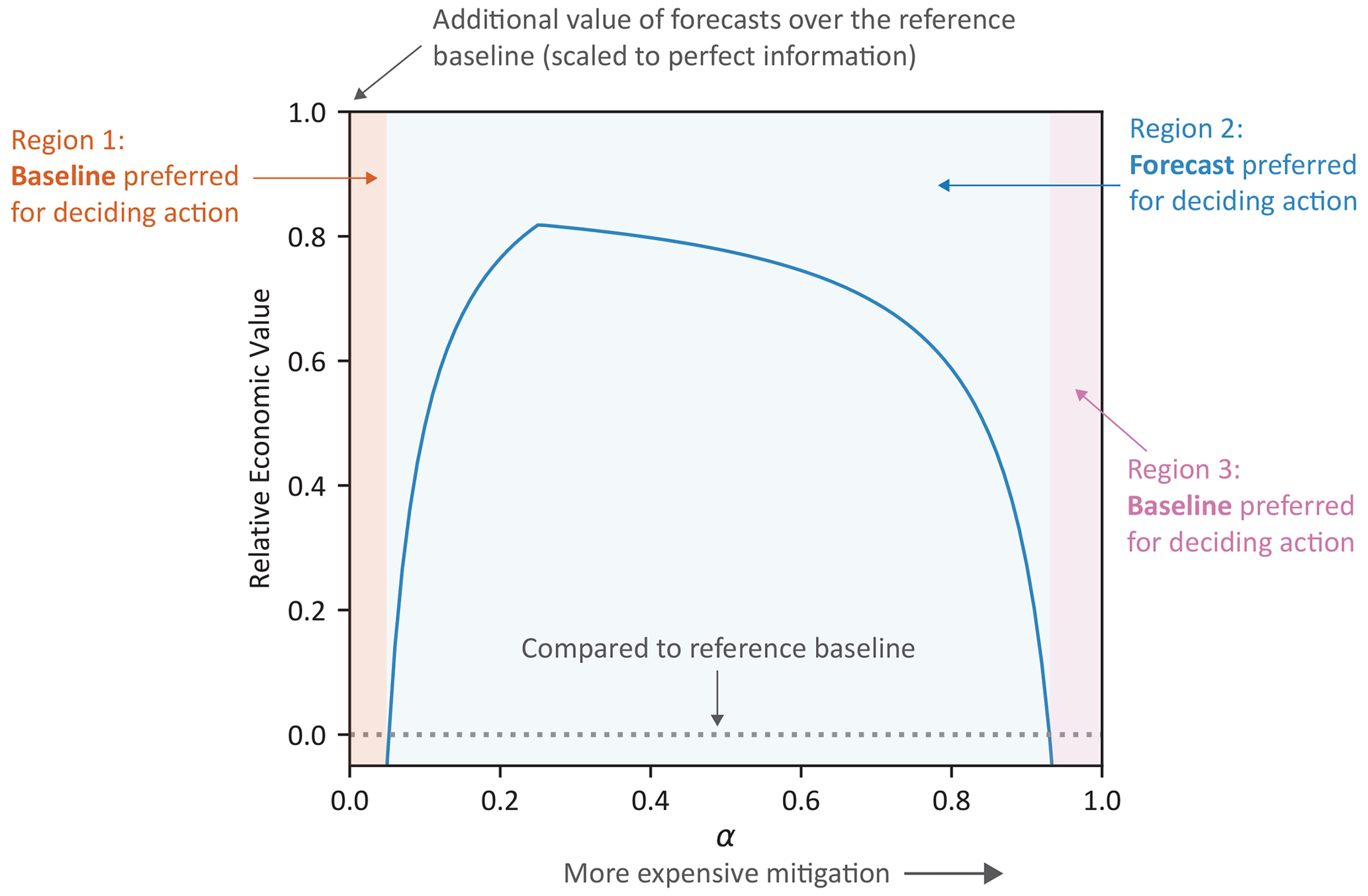
Figure 1 Illustrative value diagram with key features annotated with three key regions of α noted. Positive REV for users in region 2 indicates the forecasts should be preferred to the baseline when making the decision under analysis. Negative REV for users in region 1 and 3 indicates the baseline should be preferred.

2.1.2 REV with probabilistic forecasts

Constructing a value diagram using Eq. (2) is only possible with binary forecasts, so an additional step is required to convert probabilistic forecasts into categorical forecasts to quantify their value, as follows:

1. Introduce a critical probability threshold p_τ to convert the probabilistic forecast into a deterministic forecast using the quantile function.

2. Construct a categorical forecast and contingency table from this deterministic forecast and apply Eq. (2) over a range of α as before.

3. Repeat step 1 and 2 for many probability thresholds over the range $\mathrm{0}{\le }_{\mathit{\tau }}\le \mathrm{1}$ to form a set of possible REV values for each value of α.

4. Take the maximum value from this set for each value of α to construct a single curve that envelopes the many curves from each value of p_τ.

5. This envelope is then considered to represent the value of the forecast system.

Constructing an envelope to represent the forecast value of the system in step 4 can lead to a problematic interpretation. It implicitly assumes that the user will always self-calibrate to select the best critical threshold p_τ for their decision before the event has occurred. This is impractical and the method therefore leads to an overestimation of the expected forecast value. This envelope could alternatively be interpreted as the maximum attainable forecast value. The impracticality of this method is well understood (Zhu et al., 2002) but frequently ignored when applied in practice.

Step 1 of the approach models how users commonly make decisions using probabilistic forecasts. That is, before the event has occurred (ex ante), a user will choose a probability threshold that represents the degree of certainty they require to act. If the forecast probability of the event occurring is larger than this threshold, then they will act. We refer to this as the threshold approach.

Alternatively, one could set the critical probability threshold equal to α. This approach assumes that the user will self-calibrate based on an awareness of their specific α value (Richardson, 2000). When forecasts are perfectly reliable, this approach is equivalent to the maximum forecast value from step 4 (Murphy, 1977). Forecast systems are not perfectly reliable however, even with contemporary post-processing methods (M. Li et al., 2016; Woldemeskel et al., 2018; McInerney et al., 2020). The realised value curve will therefore lie below the maximum value curve when applied to real-world forecasts. To the best of our knowledge, studies of real-world decisions using this alternative approach (p_τ=α) have not been reported in the published literature.

2.2 Expected utility theory approach

Matte et al. (2017) introduced a method to quantify forecast value based on expected utility maximisation with a state-dependent utility. The method is flexible enough to model binary, multi-categorical, and continuous-value decisions, along with risk-averse users. The method assumes that decisions of how much to spend on mitigating damages are based on the forecast probability that the event will occur. We will refer to this approach to decision-making as the optimisation approach to contrast it with the threshold approach.

For a general decision problem with multiple possible future states of world, the following equation specifies the von Neumann–Morgenstern expected utility U for a single time step t over M states:

$$\begin{array}{}\text{(4)}& U_t\left(E_t\right)=\sum _{m=\mathrm{1}}^M{p}_{t,m}\mathit{\mu }\left(E_t\left(m\right)\right),\end{array}$$

where p_t,m is the probability of state m occurring in time step t and E_t(m) is the outcome associated with that state. The outcome is typically, but not necessarily, in monetary units. A utility function μ(⋅) maps the outcome to a utility. This utility represents an ordinal value that the user gains from that outcome occurring. The expected utility can be considered a probability weighting of the transformed outcomes of all possible states of the world.

Risk aversion is represented by the concavity of μ(⋅), such that when a user is risk-averse, the utility gained from an extra dollar is less than the utility lost when losing a dollar (Mas-Colell, 1995); see Fig. 3b for examples of μ(⋅) used in our experiments with different levels of risk aversion. Therefore, on average, the risk is only worth taking when the probability of gaining an extra dollar is more likely than losing a dollar; this is known as the probability premium. Absolute risk aversion is suitable for the comparison of options whose outcomes are absolute changes in wealth and relative risk aversion where outcomes are percentage changes in wealth. The degree of aversion could be constant, increasing, or decreasing with respect to wealth. A consumer or investor generally takes more risks as they become wealthier, and their preferences can be reasonably approximated by decreasing absolute risk aversion.

Matte et al. (2017) assumes that on average a public agency water manager is more likely to exhibit constant absolute risk aversion (CARA). For example, we assume that the managers preference for precise forecasts (risk aversion) remains fixed even if the possible losses from one decision are larger than another decision. In this case, a utility function satisfying these properties can be defined by

$$\begin{array}{}\text{(5)}& \mathit{\mu }(E;A)=-{\displaystyle \frac{\mathrm{1}}{A}}\exp (-A\cdot E),\end{array}$$

where the parameter A is the Arrow–Pratt coefficient of absolute risk aversion and E is the economic outcome (Mas-Colell, 1995). Babcock et al. (1993) cautions against interpreting the risk aversion coefficient directly and notes the importance of considering how perception of risk aversion depends on the possible loss. A more interpretable measure which allows comparison between studies with different losses is the risk premium; the proportion of loss a user would pay to eliminate a decision and replace it with a certain outcome (Pratt, 1964). The method introduced here can use any utility function, such as constant relative risk aversion, which was used by Katz and Lazo (2011).

The economic model used in this study is a simplified version of that used by Matte et al. (2017) which determines the net outcome from a cost–loss decision. The Matte et al. (2017) method considers calibration to monetary units, damages informed by flood studies, intangible damages, and distributed spending over multiple lead times. Our method is less concerned with the absolute monetary value of forecasts for a specific decision and instead focuses on the relative value of one forecast over an alternative. This leads to a metric which is more generally applicable and comparable across different users, decisions, forecasts methods, and forecast locations. A cost–loss economic model is required to compare results with REV, and is used in this study; however, the RUV method is flexible in that any economic model could be used.

For a state of the world m at a specific time step t, with damages d_t(m), cost to mitigate the damages C_t, and amount of damages avoided b_t(m), the outcome is given by

$$\begin{array}{}\text{(6)}& E_t\left(m\right)=b_t\left(m\right)-d_t\left(m\right)-C_t.\end{array}$$

The benefit function b_t(m) specifies the damages avoided from taking action to mitigate them,

$$\begin{array}{}\text{(7)}& b_t\left(m\right)=\min \left(\mathit{\beta }\cdot C_t,d_t\left(m\right)\right),\end{array}$$

where the spending leverage parameter β controls the extra damages avoided for each dollar spent. This is a similar concept (albeit inverted) to the cost–loss ratio α in the REV metric. The damage function d_t(m) relates the states of the world to the economic damages and must be specified for the decision of interest. This economic model assumes that benefits increase linearly as more is spent on damage mitigation, followed by a loss if the spend amount is greater than the damages.

The optimal amount ${\stackrel{\mathrm{‾}}{C}}_t$ to spend at time step t can be found by maximising the expected utility following substitution of Eqs. (5)–(7) into Eq. (4),

$$\begin{array}{}\text{(8)}& \begin{array}{rl}{\stackrel{\mathrm{‾}}{C}}_t& =\underset{C_t}{\mathrm{argmax}}{U}_t\left(E_t\right)\\ & =\underset{C_t}{\mathrm{argmax}}\sum _{m=\mathrm{1}}^M-{\displaystyle \frac{p_{t,m}}{A}}\exp \left[-A\cdot \left(\min \left(\mathit{\beta }\cdot C_t,d_t\left(m\right)\right)\right.\right.\\ & \left.\left.-d_t\left(m\right)-C_t\right)\right].\end{array}\end{array}$$

This optimal spend amount for each time step must be found ex ante, that is, before the event has taken place, when the future state of the world is unknown, but a forecast is available. The probabilistic forecast (for some lead time) is used to determine the forecast likelihood of each state occurring and calculate the ex ante expected utility U_t(E_t) in Eq. (8). The optimal amount to spend on mitigation is the amount which leads to the largest ex ante expected utility.

The utility can also be calculated ex post, after the event has taken place, and a singular state of the world is known (streamflow observation). This leads to the following expression for the ex post utility after substitutions into Eq. (4):

$$\begin{array}{}\text{(9)}& \mathrm{{\rm Y}}\left(E_t\right)=\mathit{\mu }\left(\min \left(\mathit{\beta }\cdot {\stackrel{\mathrm{‾}}{C}}_t,d_t\left({\stackrel{\mathrm{‾}}{m}}_t\right)\right)-d_t\left({\stackrel{\mathrm{‾}}{m}}_t\right)-{\stackrel{\mathrm{‾}}{C}}_t\right),\end{array}$$

where Υ(E_t) is the ex post utility, ${\stackrel{\mathrm{‾}}{C}}_t$ is the spend amount that was found ex ante, and ${\stackrel{\mathrm{‾}}{m}}_t$ is the state of the world associated with the observed flow at time step t. The ex post utility quantifies the benefit a user would have gained if they spent ${\stackrel{\mathrm{‾}}{C}}_t$ on mitigating the damages which occurred as a result of the observed flow. It is important to note that since utility is an ordinal quantity that represents a user's preference over the possible decision outcomes, the utilities can be compared but the actual value is non-interpretable. The ex post utility is used in the RUV metric introduced in Sect. 3.

Three ex post metrics were used in Matte et al. (2017) to quantify forecast value using spend amounts found ex ante. They use economic variables (utility, avoided losses, and amount spent) averaged over forecasts spanning an historical period. None of these metrics are equivalent or directly comparable to REV, and their results were not parameterised by an equivalent of the cost–loss ratio. The mathematical form and interpretation of these three metrics are included in Sect. S3.

Expected utility theory can be used to model more decisions with more realism than is possible with the strong assumptions of REV. However, the economically relevant metrics and parametrisation used to quantify forecast value by Matte et al. (2017) pose a challenge when comparing the outcomes from the two methods.

3 Relative utility value

This section introduces a new metric which allows direct comparison of the results quantified by the two alternative forecast value approaches described in Sect. 2. It aligns the two approaches and allows comparison using the value diagram, which is familiar to the environmental modelling verification community and a compelling communication tool. RUV is inspired by REV and skill scores, but with terms based on the ex post expected utility.

$$\begin{array}{}\text{(10)}& \mathrm{RUV}={\displaystyle \frac{\underset{t\in T}{\mathbb{E}}\left[\mathrm{{\rm Y}}\left(E_t^{\mathrm{r}}\right)\right]-\underset{t\in T}{\mathbb{E}}\left[\mathrm{{\rm Y}}\left(E_t^{\mathrm{f}}\right)\right]}{\underset{t\in T}{\mathbb{E}}\left[\mathrm{{\rm Y}}\left(E_t^{\mathrm{r}}\right)\right]-\underset{t\in T}{\mathbb{E}}\left[\mathrm{{\rm Y}}\left(E_t^{\mathrm{p}}\right)\right]}},\end{array}$$

where $\underset{t\in T}{\mathbb{E}}\left[\mathrm{{\rm Y}}\right(E_t^{\cdot }\left)\right]$ is the expected value of the ex post expected utility from Eq. (9) over a set of observations and either forecast (f), reference baseline (r), or perfect information (p). A nice feature of RUV is that it uses the whole probabilistic forecast and does not first convert it to a deterministic forecast like REV.

RUV has all the benefits and familiarity of REV but is a more flexible way to quantify forecast value. Any economic model or form of risk aversion can be used to construct the expected utility terms required by RUV because it is built on the expected utility theory framework. In this paper, we focus on the method with the economic model detailed by Eqs. (6) and (7) and risk aversion in Eq. (5). If RUV is parameterised using $\mathit{\beta }=\frac{\mathrm{1}}{\mathit{\alpha }}$ and visualised on a value diagram, it can be interpreted in the same way as an REV curve. The flexibility of the utility framework allows the user to make explicit choices about suitable approximations to model the decision problem. This can be accomplished by modifying the economic model, damage function, and risk aversion through Eqs. (5)–(7) when used to calculate RUV. These assumptions can then be evaluated and extended with additional information if available. Unlike REV using Eq. (2), additional evaluation information is available for each time step, such as the amount spent, damage avoided, and economic utility. This may benefit a user applying alternative economic models and tuning damage functions to match real-world data, as they would require the amount spent and damages incurred at individual time steps to determine if the components are behaving as expected. Additionally, a user who has finite funds to spend on mitigation and wants to determine when their budget will be exhausted would require investigation of spend and damage amounts at individual time steps.

3.1 Relationship between RUV and REV

Figure 2 contrasts the processes used by REV and RUV to quantify the value of probabilistic forecasts. Note that RUV uses the same inputs as REV and leads to the same output, however RUV allows the economic model, damage function, and risk aversion to be explicitly specified. The internal process is very similar, except RUV maximises utility rather than minimises expense.

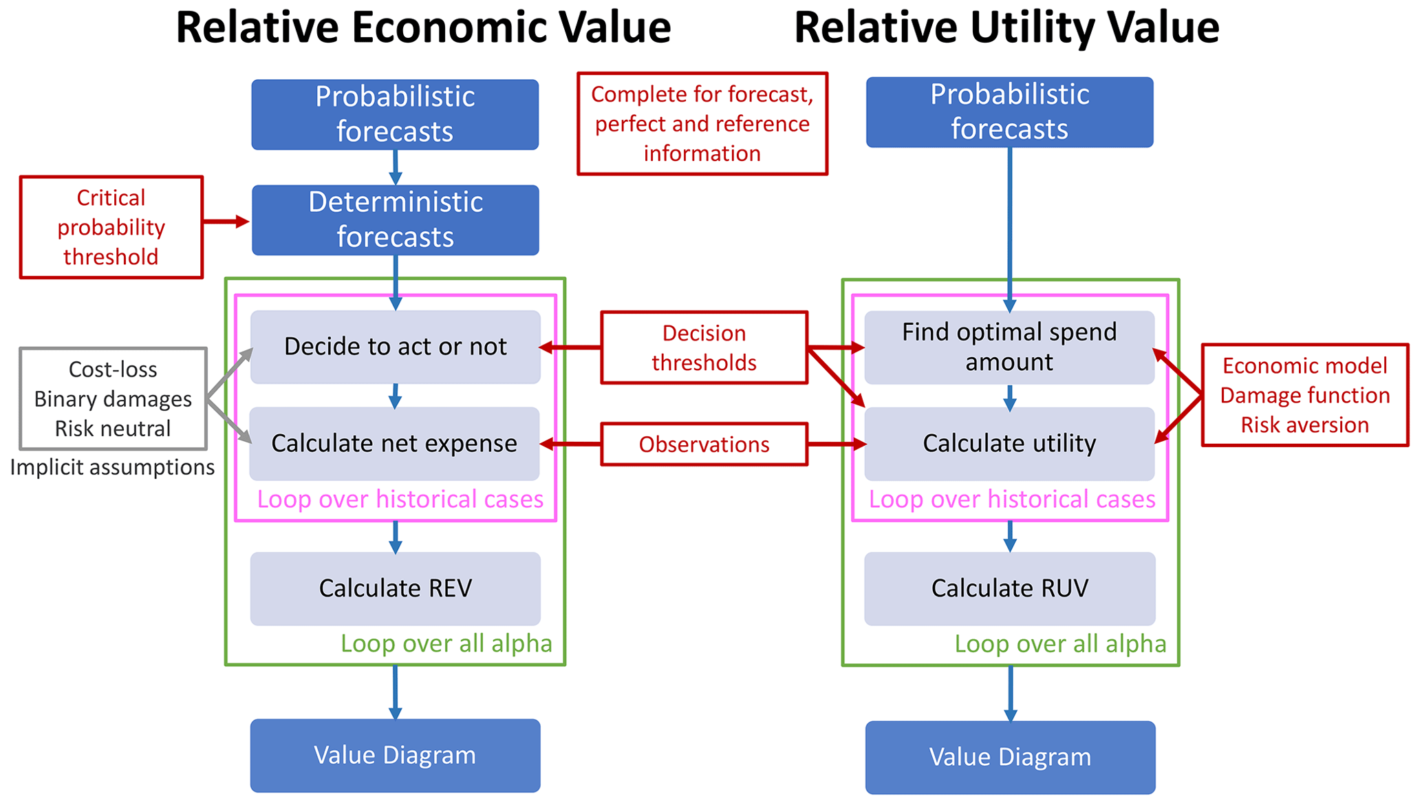
Figure 2 Flowcharts showing the process followed to quantify the value of probabilistic forecasts using either RUV with an optimisation approach to decision-making or REV using the threshold approach with a specific critical probability threshold. The sub-processes in the pink boxes are repeated for forecast, perfect, and reference information before being used to calculate REV and RUV. In practice, REV is calculated using Eq. (2), which is based on a contingency table with an assumption that it has converged to the long-run performance of the system.

Unlike REV, there is no analytical solution for RUV due to the optimisation step in Eq. (8) unless assumptions are placed on the decision context. When the following five assumptions are applied to RUV, it is equivalent to REV:

1. Binary damage function is used, which is a positive value for the losses above the decision threshold and 0 otherwise.

2. Users are risk neutral as specified by a linear utility function.

3. Forecasts are deterministic with the probability of flow above the threshold, always either 1 or 0.

4. The historical frequency of the binary event is used as the reference baseline.

5. All possible losses are avoided.

The mathematical justification for these assumptions and a proof of the equivalence is detailed in Appendix A and the Sect. S2. Note that when applying these assumptions, the core RUV method illustrated in Fig. 2 remains the same but the probabilistic forecast is first converted to a deterministic forecast. Table 2 summarises how decision concepts are represented in each forecast value method and demonstrates the enhanced flexibility of the RUV metric.

4 Illustrative case study

An illustrative case study is used to demonstrate the application of RUV for quantifying the value of sub-seasonal streamflow forecasts. A series of experiments is used to explore the sensitivity of forecast value to some aspects of decision context, specifically the decision types, users with different relative expense of mitigation and different levels of risk aversion, and decision-making approaches. A targeted approach is adopted to contrast the RUV and REV methods and illustrate the impact of decision characteristics, rather than an exhaustive evaluation of the value of the specific forecasts used.

4.1 Study region and catchment

Our case study explores the value of subseasonal streamflow forecasts at the water level station Biggara (401012) on the Murray River in the southern Murray–Darling Basin, Australia.

Agencies operating in the southern Murray–Darling Basin of Australia, such as the Murray–Darling Basin Authority (MDBA) and Goulburn–Murray Water (GMW), make releases from storages, which have impacts far downstream. Storage management decisions may benefit from subseasonal forecasts, with lead times out to 30 d, and assist Enhanced Environmental Water Delivery (Murray–Darling Basin Authority, 2017). Currently, when operational decisions are informed with probabilistic forecasts, the threshold approach is used with a set of fixed critical probability thresholds, and a degree of risk aversion is implicitly assumed (personal correspondence with MDBA). As far as the authors are aware, the relative value of streamflow forecasts for these decisions and user characteristics has not been previously quantified.

The Biggara station has particular significance for water resource management in this region as it is located upstream of Hume Dam, a major reservoir used for environmental water releases, irrigated agriculture, and town supply. It is in a temperate region, has a contributing area of 1257 km², a mean rainfall of 1158 mm yr⁻¹, and mean runoff of 361 mm yr⁻¹.

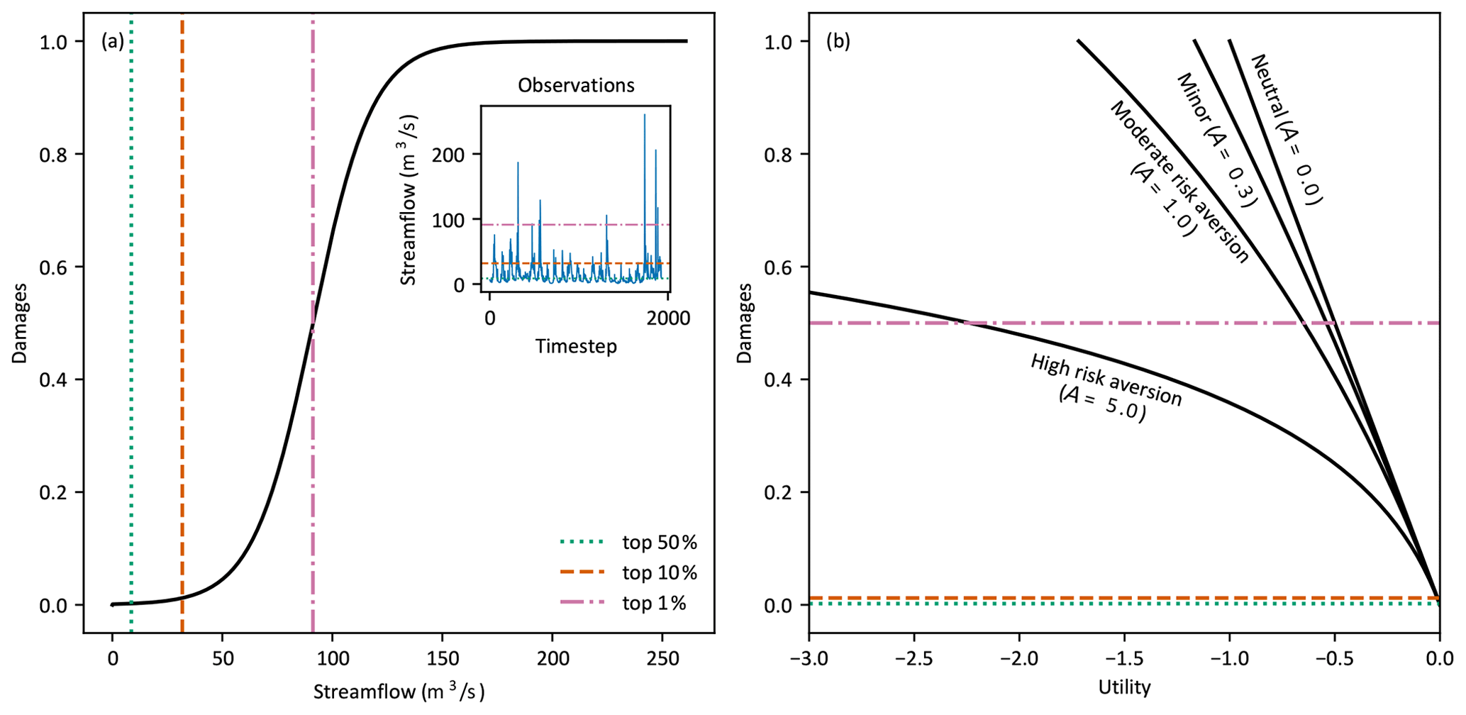
Figure 3 (a) Example damage function used in the illustrative case study based on a logistic curve with an inflection point at the top 1 % of observed flow and (b) corresponding CARA utility function with four levels of risk aversion (limited to $-\mathrm{3}\le \mathrm{utility}\le \mathrm{0}$ and aligned at zero utility for visual clarity).

4.2 Streamflow forecasts

Daily streamflow forecasts are generated using the following method which demonstrated good performance at subseasonal time horizons in earlier studies (McInerney et al., 2020, 2022). We generated 30 d ensemble forecast time series (100 members) starting on the first of each month over the period 1991 to 2012. Raw streamflow forecasts were simulated using the GR4J rainfall–runoff model (Perrin et al., 2003), forced by rainfall from the Australian Community Climate and Earth-System Simulator Seasonal (Hudson et al., 2017) that had been pre-processed using the Rainfall Post-Processing for Seasonal forecasts method (Schepen et al., 2018), and potential evapotranspiration from the Australian Water Availability Project (Jones et al., 2009). Final streamflow forecasts were generated by post-processing the raw streamflow forecasts using the Multi-Temporal Hydrological Residual Error (MuTHRE) model (McInerney et al., 2020). Post-processing ensured that the statistical properties of the streamflow forecasts closely match the streamflow observations. The MuTHRE model was chosen for post-processing because it provides “seamless” forecasts that are (statistically) reliable and sharp across multiple lead times (0–30 d) and aggregation timescales (daily to monthly). Further information on the forecasts used in this study can be found in McInerney et al. (2020), and further method improvements to enhance seamless performance in McInerney et al. (2021).

4.3 Decision types

Decisions involving more than two flow classes are an essential feature of many real-world decisions (see examples in Sect. 1). Three types of decisions are considered in the illustrative case study: (i) binary decisions with flow above a single threshold, either the top 25 % of top 10 % of the observation record; (ii) multi-categorical decisions with flow in five classes over a range of thresholds; and (iii) continuous-flow decisions using flow from whole flow regime. These thresholds are indicative of decisions that depend on moderate to high flow at Biggara, such as operational airspace management of the Hume Dam or minor inundation upstream of Yarrawonga Weir when coinciding with a dam release.

4.4 Economic damages

The relationship between damages and flow in Eqs. (6) and (7) when applying the RUV metric is specified using a non-dimensional logistic function,

$$\begin{array}{}\text{(11)}& d(q;\mathit{\delta },k,\mathit{\varphi })={\displaystyle \frac{\mathit{\delta }}{\mathrm{1}+\exp (-k(q-\mathit{\varphi }\left)t\right)}}.\end{array}$$

The logistic function can be parameterised to have very similar behaviour to the Gompertz curve used in flood damage studies and used by Matte et al. (2017), with d(q) representing the cumulative damages incurred from all flow up to q (C. Li et al., 2016). It was parameterised to reasonably characterise losses from high flow events; no damages when flow is zero, increasing quickly from around the top 20 % of flow, and approaching 1 at very high values above the top 1 % of flow (see Fig. 3a). These assumptions were reproduced with the following parameter set; δ=1, k=0.07 and ϕ equal to the value corresponding to the top 1 % of observed historical flow.

4.5 Risk aversion

It is difficult to precisely know a user's level of risk without a history of prior decisions. Moreover, it would be incorrect to assume that all users share the same level of risk. Therefore, a range of risk aversions have been considered to illustrate its impact on forecast value. In this study, we have used risk aversion coefficients A∈{0, 0.3, 1,5}, which correspond to risk premiums of θ≈{0 %, 15 %, 43 %, 86 %} for a CARA utility function with maximum losses of δ=1 (Babcock et al., 1993). Figure 3b shows that the curvature of μ(⋅) increases with increasing risk aversion, and this leads to an increasingly rapid decline in utility from damages. The four risk aversion coefficients represent users who are neutral, minorly, moderately, and highly risk averse, respectively. When risk premiums are considered, our range of risk aversion coefficients is similar to those used by Tena and Gómez (2008) and Matte et al. (2017). Finding appropriate values of risk aversion for a specific user is beyond the scope of this study but would be highly beneficial in user-focused forecast value studies.

Table 3 Dimensions of forecast value problem used for each figure. The key dimension introduced in each experiment is highlighted with italic text.

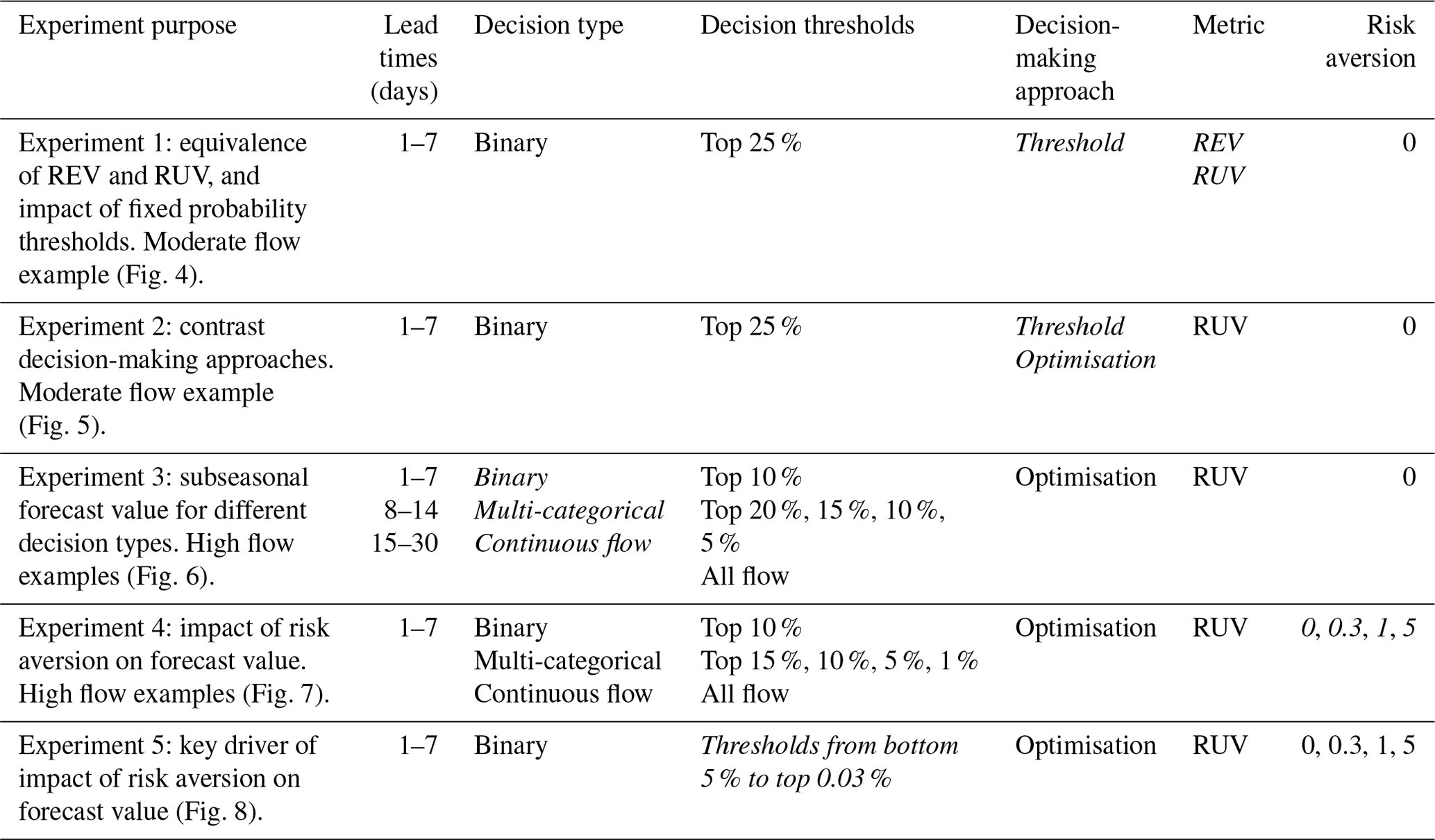
4.6 Experiments

The value of the subseasonal forecasts are quantified using the RUV and REV metrics. Experiments are performed over the dimensions of forecast lead time, decision type, decision-making approach, metric, and user risk aversion. Streamflow forecasts from multiple daily lead times were grouped together to quantify forecast value over 7 and 14 d forecast horizons. Grouping lead times together simplifies the introduction of RUV and comparison of its salient features with REV; however, for practical applications, there may be benefits for evaluating forecast value at specific lead times of interest. A fixed climatology based on all observed values in the record is used for the reference baseline of RUV to align with that used in REV. Table 3 summarises the specific attributes used for each figure, with the key dimension highlighted as italic text.

5 Results

5.1 Experiment 1: equivalence of RUV and REV and impact of fixed probability threshold

In Experiment 1, forecast value has been quantified using REV and RUV with the assumptions detailed in Sect. 3.1: binary damage function, risk-neutral user, deterministic forecasts, event frequency for reference baseline, and all losses avoided. As expected, Fig. 4 demonstrates that the results are identical between the two methods.

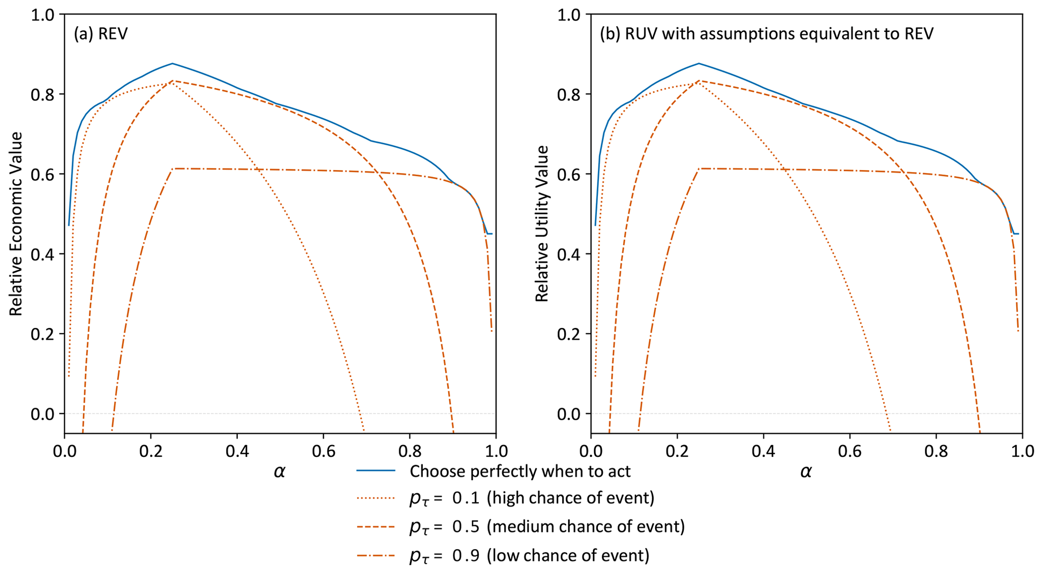
Figure 4 Forecast value quantified using (a) REV and (b) RUV with assumptions enforced and the threshold approach for decision-making. A binary decision of flow exceeding the top 25 % of observations, subseasonal forecasts from the first week of lead times, and a risk-neutral user. Critical probability thresholds for the four curves are the value leading to maximum forecast value and the 0.1, 0.5, and 0.9 forecast quantile corresponding to acting when there is a high, medium, or low chance of event occurring, respectively.

We now explore the detrimental impact on forecast value of using the threshold approach to convert probabilistic forecasts to deterministic forecasts. Any forecast value method using the threshold approach needs to select a critical probability threshold p_τ to convert probabilistic forecasts to deterministic forecasts. Figure 4 includes three curves corresponding to decisions made with different thresholds. The blue line shows the value obtained when the threshold p_τ is chosen to maximise that value at each α (see Sect. 2.1.2). This is an upper limit that cannot be obtained in practical situations because it implies a user has either perfect foresight or a perfectly reliable forecast, and p_τ=α will lead to maximum value if the forecast is perfectly reliable (Richardson, 2000). The orange lines show how the choice of p_τ can have a dramatic impact on the value of forecasts for a decision, with the dotted line showing forecast value when p_τ=0.1, the dashed line when p_τ=0.5, and the dash–dot line when p_τ=0.9. RUV is negative for some regions of α, which indicates that those users should prefer the climatological baseline rather than the forecasts when making decisions.

This result clearly shows that to extract the most value from forecast information, a user needs to consider their relative expense of mitigation α when choosing p_τ. For example, when a user with α=0.8 uses p_τ=0.9, they gain significant value from the forecasts (RUV≈0.6), but if they use p_τ=0.1, their outcome using forecasts is worse than using the reference baseline (RUV<0), while for a different user with α=0.1, the opposite is true. This critical dependence of value on p_τ is an established finding for REV (Richardson, 2000; Murphy, 1977) and is not specific to this example; here, we illustrate that RUV reproduces it. Figure 4 additionally shows that the value diagram used with REV remains a compelling way to visualise how RUV forecast value varies for different users.

This result, and the derivation in Appendix A and Sect. S2, demonstrates that RUV and REV are equivalent when appropriate assumptions are imposed. It shows that REV can be considered a special case of the more general RUV metric.

5.2 Experiment 2: contrasting the threshold approach and optimisation approach for decision-making

Figure 5 adds two more forecast value curves, generated using RUV, to Fig. 4. The black line shows value when the optimisation approach is used to make spending decisions with the subseasonal forecasts (detailed in Sect. 2.2) and the pink line shows value when the threshold approach is used with p_τ=α. The result demonstrates that making decisions using either approach provides close to the maximum value possible for all users (different values of α). This contrasts dramatically with the threshold approach using specific fixed values for p_τ (orange lines) which only provides maximum value for a very small range of users.

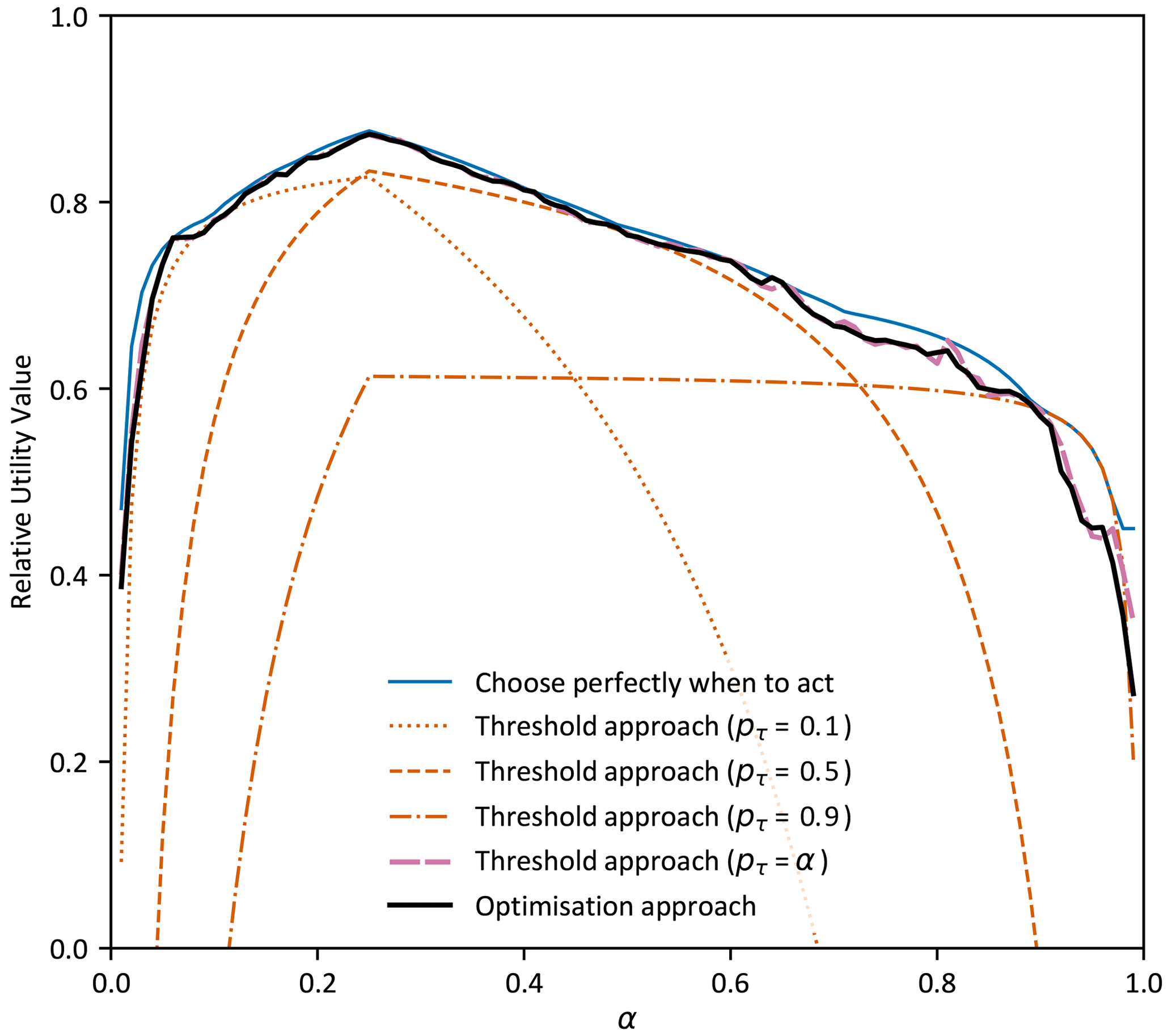
Figure 5 Forecast value quantified using four different approaches to decision-making: the optimisation approach and the threshold approach with either perfect critical probability thresholds, specific critical thresholds, or the critical threshold set equal to the α value. A binary decision of flow exceeding the top 25 % of observations was used, with subseasonal forecasts from the first week of lead times and a risk-neutral user. Specific critical thresholds are the 0.1, 0.5, and 0.9 forecast quantile corresponding to acting when there is a high or low chance of the event occurring, respectively.

Investigations (not shown) indicated that the optimisation and p_τ=α curves (black and pink lines) are non-smooth because of the limited number of events in the observation record, and the small difference between the black and pink lines is due to sampling errors from to the relatively small ensemble size. It is notable that forecast value from these two different decision-making approaches are essentially equivalent as illustrated by the closeness of the black and pink lines in Fig. 5. Additional analysis (not shown) found this equivalence to be robust to the type of decisions (binary, multi-categorical, or continuous flow) but not equivalent for risk-averse users.

Figure 6 Forecast value for (a) binary decision of flow exceeding the top 10 % of observations, (b) flow within five classes with thresholds at the top 20 %, 15 %, 10 %, and 5 % of observations, and (c) continuous-flow. Decisions are made using the optimisation approach for decision-making with a risk-neutral user, and subseasonal forecasts for the first, second, and combined third and fourth weeks of lead times.

5.3 Experiment 3: comparing forecast value for different types of decisions

Figure 6 presents results for binary (blue lines), multi-categorical (orange lines), and continuous-flow decisions (green lines) with forecast lead times in separate panels. RUV was calculated for the daily subseasonal forecasts with lead times pooled from the first week (Fig. 6a), second week (Fig. 6b), and third and fourth weeks combined (Fig. 6c). The user is assumed to be risk neutral, and the optimisation approach was used. Overall, the forecasts provide excellent value for these three different decision types over all time horizons (max. 30 d), implying that any user would likely benefit from using the forecast information over the reference baseline. Peak RUV is over 0.8 in the first week for all decision types, and close to 0.7, 0.6, and 0.5 in subsequent weeks for binary, multi-categorical, and continuous-flow decision types, respectively. Regardless of the decision type or lead time, forecasts provide maximum value for users with α close to the probability of the most damaging flow class occurring. For example, for the binary decision, the peak RUV value is located at α=0.1, which corresponds with the event frequency of decision threshold used (top 10 % of flow).

Figure 6 shows that there is important variation in RUV for different decision types. These differences in RUV for different decision types are more pronounced for larger values of α and at longer lead times. For example, for users with α>0.6 (lead time week 2), the RUV is below zero for the binary decision type, but not the multi-categorical or continuous-flow decision types. This suggests the users should prefer the reference baseline for the binary decision and prefer forecasts for the multi-categorical and continuous-flow decisions. This highlights the importance of calculating forecast value using the decision type which matches the decision being assessed.

It is notable that for higher values of α, the value of forecasts in weeks 3 and 4 is higher than week 2. While differences are minor, they interestingly appear robust over the multiple decision types in this case study. The reduced value of forecasts could possibly be due to lead-time-dependent differences in forecast reliability and decreasing sharpness of the forecast ensemble at longer lead times. Another notable feature is that forecast value at small α is enhanced for continuous-flow decisions relative to the other decision types. This seems to be because large damages from infrequent extreme events are more adequately mitigated in continuous-flow decisions because a correspondingly large amount is spent when they are forecast correctly.

5.4 Experiment 4: impact of risk aversion

Experiment 4 contrasts forecast value for a risk-neutral user against three different levels of risk aversion for binary, multi-categorical, and continuous-flow decisions. The results presented in Fig. 7 for the RUV metric (first row) as well as the overspend (middle row) and utility-difference metrics (last row) used by Matte et al. (2017) provide insight into the spending decisions and utility, respectively. By varying A in Eq. (5), risk aversion is found to have a significant impact on the value of forecasts for highly risk-averse users making continuous-flow decisions, a moderate impact for multi-categorical and continuous-flow decisions (except for highly risk-averse users), and a minor impact for binary decisions (see Fig. 7, first row). Increased risk aversion shifts the RUV curve toward users with higher α, suggesting that risk-averse users with more expensive mitigation would benefit more from using forecasts to make their decisions.

Figure 7 RUV, overspend, and utility difference for different levels of user risk aversion for a binary decision of flow exceeding the top 10 % of observations (a, d, g), flow within five classes with thresholds at the top 15 %, 10 %, 5 %, and 1 % of observations (b, e, h), and continuous flow (c, f, i). Decisions made using the optimisation approach with subseasonal forecasts from the first week of lead times.

The overspend (Fig. 7, middle row) and utility-difference results (Fig. 7, last row) indicate that risk aversion has a minor impact on the spending decisions and the resultant utility, except for highly risk-averse users making continuous-flow decisions. The overspend panels show that regardless of risk aversion, on average, a user will spend more than necessary when their cost of mitigation is small relative to the potential avoided losses (small α). Conversely, when α is large, they will underspend on average. When risk aversion is increased, users spend increasingly more.

The utility-difference panels (Fig. 7, bottom row) show that decisions made using forecasts provide users less utility than decisions made using perfect information, and this decrease in utility increases with risk aversion. As utility is an ordinal measure, it is only meaningful to interpret differences within Fig. 7g, h, and i, not between them. This highlights a benefit of the overspend and RUV metrics which are comparable across decision type.

5.5 Experiment 5: mechanism behind the varying impact of risk aversion

It is notable that the impact of risk aversion in Fig. 7 is different for each decision type; minor for the binary decisions, moderate for multi-categorical and continuous-flow, and particularly enhanced for highly risk-averse users. Experiment 5 investigates the mechanism behind this. Figure 8 presents the difference in RUV between risk-averse and risk-neutral users (y axis) for a binary decision at a single value of α (α=0.2). The binary decision threshold (x axis) is varied from 2–225 m³ s⁻¹ (bottom 5 % to top 0.03 %), and decisions are made using the optimisation approach with subseasonal forecasts from the first week of lead times. This contrasts with the binary decision in experiment 4, where the decision threshold is fixed at 32 m³ s⁻¹ (top 10 %) and α is varied.

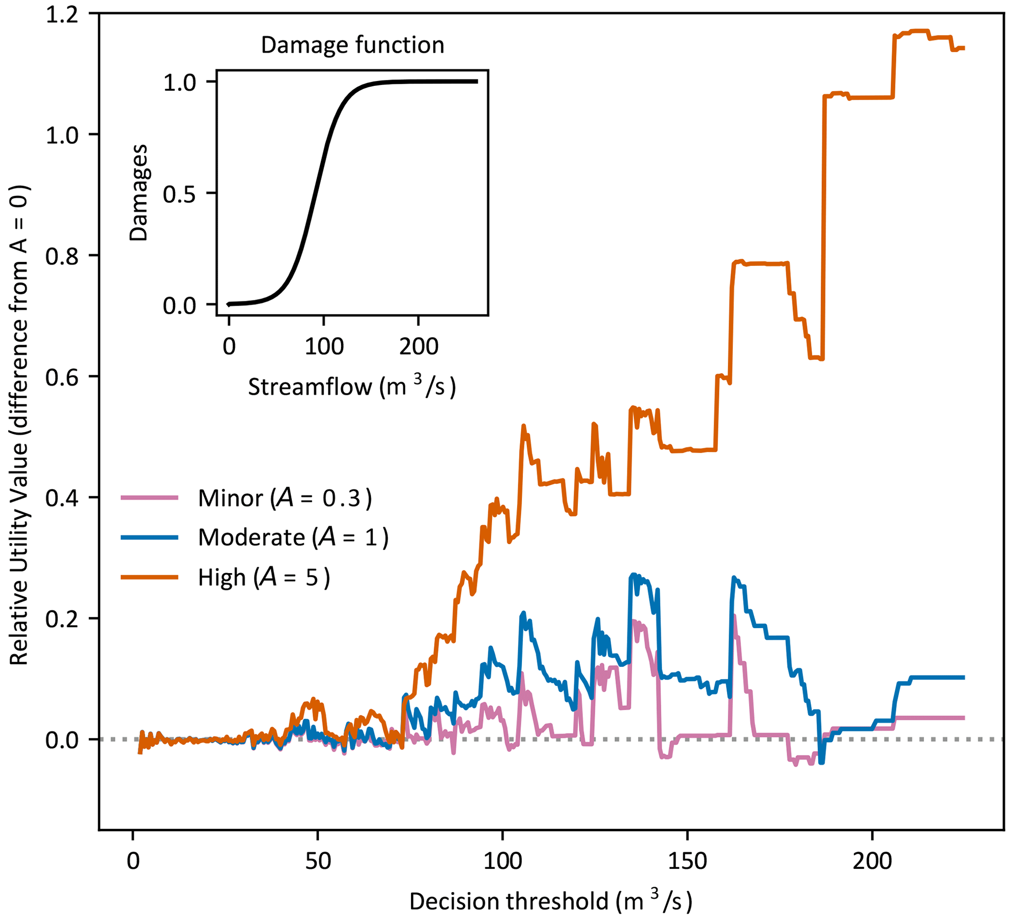
Figure 8 Difference in RUV between risk-averse (A>0) and risk-neutral (A=0) users (y axis) for a binary decision at a single α value (α=0.2). The binary decision threshold (x axis) is varied from 2–225 m³ s⁻¹ and decisions are made using the optimisation approach with subseasonal forecasts from the first week of lead times.

Below a critical decision threshold of approximately 70 m³ s⁻¹ (top 2 % flow), the difference in RUV between any level of risk aversion and risk neutrality is negligible. Above this value, an increasing difference is clear, particularly in the highly risk-averse case, with risk-averse users gaining more value from the forecast information than risk neutral. This finding was consistent for multi-categorical decisions of any number of flow classes, all lead times, and all values of α except at extreme high and low values (not shown). The specific experimental values (binary decision, α=0.2, first week lead time) were chosen as a representative example, and the findings apply for other experimental values. It demonstrates that the decision thresholds used, specifically in relation to the damage function, are the key drivers behind the impact of risk aversion regardless of the decision type. The difference in impact of risk aversion across the different decision types in Fig. 7 can therefore be explained by the specific decision thresholds used in relation to this critical value. The binary decision threshold of 32 m³ s⁻¹ used in experiment 4 was less than the critical value of 70 m³ s⁻¹, and only a minor impact from risk aversion was found. Whereas the top decision threshold for the multi-categorical decision was 91 m³ s⁻¹, above this critical value, and a moderate impact was found. An even larger impact was found for the continuous-flow decision which includes contribution from the largest flows.

6 Discussion

Statistical forecast verification metrics have previously been used to show that the probabilistic streamflow forecasts used in this study are reliable and sharp, largely due to the post-processing method employed (McInerney et al., 2021). Other post-processing methods have also demonstrated capability to improve the reliability and sharpness of raw streamflow forecasts (Bogner et al., 2016; M. Li et al., 2016; Woldemeskel et al., 2018; Lucatero et al., 2018). However, the ability of these forecasts to improve decision outcomes has not been extensively established. Additionally, REV, the most frequently used forecast value method, can only be applied to a limited number of real-world decisions. In this paper, we developed a new forecast value method, relative utility value (RUV), which is more flexible than REV and can be applied to more decisions. The flexibility of RUV is demonstrated with an illustrative case study using probabilistic subseasonal streamflow forecasts to inform binary, multi-categorical, and continuous-flow decisions with risk-averse users. The five experiments reported in Sect. 5 systematically explore the impact of different aspects of a decision on forecast value: the forecast value method, the probabilistic decision-making approach, types of decisions, user risk aversion, and the mechanism behind varied risk aversion impact. First, we find that under certain conditions RUV and REV are equivalent, and REV can be considered a special case of the more general RUV method (see Fig. 4, Appendix A, and Sect. S2). Second, making decisions with fixed critical probability thresholds leads to maximum forecast value only for a very small set of users, and using an optimisation-based approach makes better use of probabilistic forecast information (see Fig. 5). Third, we showed that forecast value varies by both decision type and how expensive mitigation is for the user, highlighting the importance of calculating forecast value with the decision type which matches the real-world decision (see Fig. 6). Fourth, risk aversion has a varied impact (minor to moderate) on forecast value (see Fig. 7) and the degree of impact is sensitive to the decision context being evaluated. And finally, the key mechanism driving this impact is decision thresholds used relative to the damage function (see Fig. 8).

6.1 Benefits of RUV over alternatives

6.1.1 Forecast value complements forecast verification

Unlike forecast verification, forecast value considers the broader context within which decisions are made. This allows forecast producers, such as the Australian Bureau of Meteorology, to understand their user impact by evaluating service enhancements against user decisions. Forecast verification is typically a key deciding factor when determining which method or enhancement to operationalise. Quantifying the value of forecasts based on impact offers a complementary line of evidence which places the forecast user at the centre of the conversation. Because RUV encourages a dialogue between the forecast producer and user to define the full decision context, it may enhance communication and service adoption. For forecast users, it provides a new capability: an evidence-based approach to decide which forecast information and decision-making process will improve their outcomes. For example, the illustrative case study in Sect. 5 indicates that subseasonal forecasts at Biggara offer better value than reference baseline in almost all cases, and that an optimisation approach is beneficial when deciding to take early action to mitigate damages from a high flow event a few weeks ahead (see Figs. 5 and 6).

6.1.2 RUV is more flexible than REV

RUV can model more decisions with sufficient realism than REV because it explicitly specifies decision type, risk aversion, economic model, and decision-making approach. Real-world decisions may be binary, multi-categorical, or based on continuous flow, and using a binary model (as in REV) in all cases will provide a misleading measure of forecast value for non-binary decisions. Figure 6 shows that neglecting this would have important implications for users; forecasts beyond week 2 should be used for the multi-categorical and continuous flow but not for the binary decision (when α>0.6). Similarly, neglecting the realism of other aspects of the decision may lead to other misleading conclusions. The flexibility of RUV allows the user to decide how much realism to include in the forecast value assessment depending on the information available and tailor it to the decision context.

6.1.3 RUV evaluates forecast value conditioned on how expensive a user's mitigation is

Unlike single-valued metrics, common in traditional forecast verification, RUV is evaluated for wide range of users' experiences, as is shown in the value diagram (Fig. 1). This offers valuable insight that would otherwise be hidden. In particular, it is useful for forecast producers who can quickly compare one forecast system to another over a range of users with different relative expenses of mitigation (α). However, this does make it comparatively more difficult to summarise and aggregate. To assist interpretation for a single decision-maker, it is important the decision-maker narrows the range of α that is relevant to their decision by considering how expensive their mitigation of damages is.

6.2 Implications of case study experiments

6.2.1 Optimisation-based decision-making is better than fixed critical probability thresholds when using probabilistic forecasts

Figure 5 demonstrates that a specific critical probability threshold will only be optimal for a specific value of α and suboptimal for all other values. When a user is choosing between using the forecast or the reference baseline, they may choose incorrectly if their critical probability threshold is not aligned with their relative expense of mitigation. This incorrect choice will be due to a deficiency in the threshold approach to decision-making rather than the forecast information. This RUV-based finding is well supported by the REV literature (Richardson, 2000; Wilks, 2001; Zhu et al., 2002; Roulin, 2007). A perfect critical probability threshold is typically used with REV (Fig. 4); unfortunately, this is not possible to achieve in practice and the quantified value is unrealistically high. Matte et al. (2017) introduced an optimisation approach and we extended it here to further evaluate the impact on forecast value. This flexible approach makes best use of the forecast information available, and for risk-neutral users is equivalent to the threshold approach when the threshold is set equal to the user's relative expense of mitigation α (Fig. 5). When forecasts are reliable, this method yields value that is very close to the maximum possible, and forecast users may consider adopting this alternative approach for daily operational decisions. For this approach to be adopted for operational decision-making, a decision support system would be required to calculate the optimal amount to spend on preventative mitigation each time a new forecast is issued. This implies a suitable economic model is available for the decision and can be used for this calculation.

6.2.2 Forecast information is more valuable for risk-averse users making high-stakes decisions

Figure 7 (middle row) demonstrates that for a given forecast, a more risk-averse user spends more to mitigate a potential damaging event than a less risk-averse decision-maker, all else being equal. This behaviour is consistent with their preference for risk aversion because it leads to a more certain result, with the net outcome equal to the spend amount whether the event occurs or not. There is a large difference in impact of risk aversion for the different decision types however, and Fig. 8 summarises the findings of an investigation into this. Decision thresholds corresponding to very high flows lead to a larger impact. This finding explains why risk aversion has a large impact for the continuous-flow decision, spanning the whole regime, and a negligible impact for the binary decision with a single moderately high decision threshold. It suggests that for a risk-averse user making a high-stakes decision, forecasts become increasingly more valuable as the potential damages become larger. It may also explain apparently contradictory findings on the impact of risk aversion in the literature. Matte et al. (2017) assessed the impact of risk aversion on a multi-categorical decision (using overspend and utility metrics) and found it had a moderate impact (similar to the multi-categorical decisions shown in Fig. 7e and h). Their study used 12 uniformly spaced flow divisions over a high flow range and a damage function based on empirical flood studies, whereas this study used four widely spaced thresholds over a similar high flow range. A recent study by Lala et al. (2021) found minor impacts from risk aversion for binary cost–loss decisions with extreme rainfall forecasts, using the same expected utility maximisation framework from Matte et al. (2017), and found a similar impact to Fig. 7a. An alternative argument using reasoning from decision theory suggests that for a given risk premium, the impact should be larger when decision thresholds are closer together (Mas-Colell, 1995). However, when investigated, we found no evidence to support this for our case study experiments. Further research to better characterise the response for different decision contexts would be useful because the impact is modulated by both the decision thresholds and the specific damage function, consideration of the inherent sampling error introduced for extreme events would also be useful.

6.3 Limitations and future work

6.3.1 Exploring the impact of alternative damage functions, economic models, utility functions, and reference baselines on forecast value

This study focused on the impact of alternative decision types and risk aversion and a comparative study of RUV and REV. The foundation in expected utility theory allows us to model more decisions more realistically than REV, but it requires more information. When this information is unavailable or uncertain, the user is required to make assumptions, but it is not always clear how to best do this. One strategy is to model all decisions as binary, cost–loss, and risk neutral, and effectively convert RUV to REV. This study explores the implications of relaxing some, but not all, of those assumptions, but is limited to an analysis at a single forecast location. In particular, the damage function used was parameterised to simplify the introduction of RUV, facilitate comparison with REV, and highlight important implications for future studies. Further work will consider the impact of alternative damage functions and economic models tailored to other decision contexts. More descriptive economic models than cost–loss will be essential to consider decisions which involve non-economic intangible externalities like social, cultural, and ecological factors (Jackson and Moggridge, 2019; Expósito et al., 2020). Future studies which consider these impacts may be required to address unresolved findings in our study, such as inconsistent dependence of forecast value on lead time (see Sect. 5.3).

6.3.2 Tailoring the evaluation of forecast value to real-world decisions

For practical applications of RUV, it is advisable to calibrate the damage function, decision thresholds, economic model, decision-making approach, and reference baseline to the real-world experience of the decision-makers. This calibration will ensure the resulting forecast value is tailored to the specific decision context and will likely lead to more user trust in the results, and subsequently more appropriate use of forecast information. While the reference baseline (fixed average climatology) used in this study enabled a direct comparison of RUV with REV, we would recommend comparison against more relevant baseline forecasts for practical applications (e.g. information currently used to inform the decision being assessed).

6.3.3 Expected utility theory approximates actual decision-making, and contemporary frameworks may enhance the capability of RUV to model real-world decisions

There is general agreement, and a substantial body of evidence, that expected utility theory does not adequately describe individual choice (Kahneman and Tversky, 1979; Harless and Camerer, 1994). Many alternative models have been proposed which address these violations, such as cumulative prospect theory (Tversky and Kahneman, 1992). Future work could consider whether quantifying forecast value using a foundation built on a better model of decision-making changes the conclusions reached. Additionally, the cost–loss economic model used in this study implies that mitigation is preventative action to minimise forecast losses, with each forecast lead time and forecast update treated independently of all others. Alternative economic models and decision-making frameworks may be required to explore more realistic forms of mitigation which consider temporal dependence (see Matte et al., 2017 for an approach).

6.3.4 Exploring the relationship between forecast value and forecast skill

Roebber and Bosart (1996) found that statistical performance metrics were poor at predicting the cost–loss value of meteorological forecasts for several real-world decisions. The relationship was impacted by the user's α value, and when in aggregate, the distribution of α over all users. Using a real-time optimisation system to manage reservoir operations, Peñuela et al. (2020) quantified forecast value through improvement in pumping costs and resource availability relative to a baseline. They found a relationship between forecast value and CRPS skill score mediated by user priorities and hydrological conditions. Although a relationship exists, it is clearly mediated by the characteristics of the decision and user, and in many cases forecast skill is not a good proxy for forecast value (Murphy and Ehrendorfer, 1987; Wilks and Hamill, 1995; Roebber and Bosart, 1996; Roulin, 2007; Peñuela et al., 2020). Exploring this relationship is of interest because the decision and user characteristics are made explicit in RUV. Converting RUV to a single-value metric by placing assumptions on the distribution of α could assist and additionally allow its use as an objective function for model calibration or as a summary statistic; Wilks (2001) considers this using REV. The forecast value results of our illustrative case study are likely to be sensitive to flow characteristics and forecast uncertainty of our selected location. Future work will evaluate the value of streamflow forecast over different hydroclimatic conditions. Additionally, forecast skill (and reliability) is impacted by a forecast model's ability to reproduce seasonality and antecedent conditions. Although these are modelled well by the system used in this study (McInerney et al., 2020), their impact on forecast value was not considered in our sensitivity analysis. A future study assessing how RUV is impacted when models fail to reproduce seasonality, antecedent conditions, and other features would be a useful contribution to the field. The impact of seasonality and antecedent conditions on forecast value has not been considered in our sensitivity analysis and a future study assessing how RUV is impacted by them would be a useful contribution.

7 Conclusions

Forecast value methods aim to quantify the potential benefits that probabilistic forecasts have for water-sensitive decisions, such as operational water resource management and emergency warning services. However, the most used method to evaluate forecast value, relative economic value (REV), is only suitable for specific decisions. REV is unsuitable for many real-world decisions and when applied may lead to misleading conclusions on when to use forecasts. This paper introduces the RUV metric, which has the same interpretation as the commonly used REV metric, but is more flexible and can be applied to a far wider range of decision contexts. This is because many aspects of the decision-making process can be incorporated into RUV by the user and adjusted to match real-world decisions. These include the economic model, damage function, decision type, user risk aversion, and relative expense of mitigation.

An illustrative case study using probabilistic subseasonal streamflow forecasts in a practically significant catchment in the southern Murray–Darling Basin of Australia was used to compare the REV and RUV metrics under a range of decision contexts. The key findings from this case study were the following:

1. REV can be considered a special case of the more general RUV method.

2. Making decisions using an optimisation-based approach which uses the whole forecast distribution to determine the amount spent on mitigation makes better use of probabilistic forecast information than using a threshold-based approach with fixed critical probability thresholds.

3. Forecast value depends on the decision type, and hence it can be critically important to use a decision-type that matches the real-world decision.

4. Risk-averse users gain more value from forecasts than risk-neutral users, but the impact can vary from minor to moderate depending on the decision context.

5. Impact of risk aversion on forecast value is mediated by how large the potential damages are for a given decision.

Findings 3–5 were generally sensitive to the user's relative expense of mitigation. For example, the impact of the decision type was more pronounced for users with higher relative expenses of mitigation (α>0.6). In this case, for lead times longer than 1 week, forecast value from RUV of a binary decision was significantly lower than for multi-categorical or continuous-flow decisions. As REV is limited to binary decisions, a user making a multi-categorical or continuous-flow decision could be misled by the REV outcomes and consider not using the forecasts when they actually have significant value as demonstrated by RUV.

This paper focuses on the introduction of RUV and an exploration of its sensitivity to some aspects of decision context. Therefore, several future research directions for RUV are discussed, including (i) exploring sensitivity of forecast value to more aspects of decision context, (ii) tailoring forecast value to real-world decisions, (iii) assessing alternative frameworks for modelling decision-making, and (iv) exploring the relationship between forecast value and forecast skill.

RUV presents an opportunity to tailor forecasts and their assessment to the specific decisions, decision-making approach, characteristics, preferences, and economics of the user. It is hoped that this capability will encourage the assessment of forecast systems through the lens of user benefit and be seen as a complement to forecast verification. This may lead to increased adoption of forecasts through deeper dialogue and understanding, and ultimately to improved water resource management decisions.

Appendix A: Proof of equivalence of REV and RUV under specific assumptions

This section demonstrates the equivalence of the REV metric as detailed in Eq. (2) and the RUV metric introduced in Sect. 3 when 5 assumptions are applied to the decision context. A complete derivation is included in Sect. S2.

In a cost–loss decision problem, the two relevant states are “flow above” and “flow below” a decision threshold Q_d.

$$\begin{array}{}\text{(A1)}& \begin{array}{rl}& m=\mathrm{above}\mathrm{if}{Q}_t\ge Q_{\mathrm{d}}\\ & m=\mathrm{below}\mathrm{if}{Q}_t<Q_{\mathrm{d}}.\end{array}\end{array}$$

Assumption 1. A step damage function with binary values of 0 and L is used to specify the losses above and below the decision threshold for all time steps,

$$\begin{array}{}\text{(A2)}& d(m;L)=\left\{\begin{array}{cc}L& \mathrm{when}m=\mathrm{above}\\ \mathrm{0}& \mathrm{when}m=\mathrm{below}\end{array}\right..\end{array}$$

To calculate the net outcome when action is taken to mitigate the loss, we substitute Eqs. (7) and (A2) into Eq. (6) which leads to the following net outcomes for the two states:

$$\begin{array}{}\text{(A3)}& \begin{array}{rl}& E_{\mathrm{t},\mathrm{above}}=\min \left(\mathit{\beta }\cdot C_t,L\right)-L-C_t\\ & E_{\mathrm{t},\mathrm{below}}=-C_t\mathrm{since}\mathit{\beta }\cdot C_t>\mathrm{0}.\end{array}\end{array}$$

Assumption 2. Linear utility function is assumed which implies no aversion to risk,

$$\begin{array}{}\text{(A4)}& \mathit{\mu }\left(E\right)=E.\end{array}$$

Substituting Eq. (A3) into Eq. (4), applying the linear utility function assumption, and simplifying for only two possible states using p_t, the forecast probability of flow above the flow threshold at time t leads to

$$\begin{array}{}\text{(A5)}& \begin{array}{rl}U\left(E_t\right)& =p_t\cdot E_{t,\mathrm{above}}+\left(\mathrm{1}-p_t\right)\cdot E_{t,\mathrm{below}}\\ & =p_t\cdot \left[\min \left(\mathit{\beta }\cdot C_t,L\right)-L-C_t\right]+\left(\mathrm{1}-p_t\right)\cdot \left[-C_t\right]\end{array}.\end{array}$$

Assumption 3. Probability of flow above the threshold will always be either 1 or 0,

$$\begin{array}{}\text{(A6)}& p_t\in \mathit{\{}\mathrm{0},\mathrm{1}\mathit{\}}.\end{array}$$

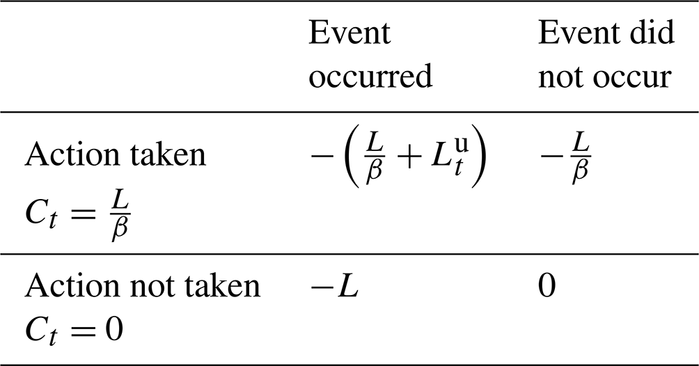
Using these assumptions and noting that the total loses at each time step are fixed and consist of avoided and unavoided components, $L=L_t=L_t^{\mathrm{a}}+L_t^{\mathrm{u}}$, we can now determine the single time step ex ante utility for the four possible outcomes. The four possible outcomes are composed of an event is forecast to occur (p_t=1) or not occur (p_t=0), and an action has therefore been taken or not, leading to Table A1.

Table A1 Ex ante utility values for a time step of expected utility theory with REV assumptions.

Applying Eq. (8) to Eq. (A5) will lead to an optimal amount ${\stackrel{\mathrm{‾}}{C}}_t$ to spend on the mitigating action for each time step. By considering that the forecast probability is always either 1 or 0 due to assumption 3 and that all costs and losses are positive values, we can derive that for any time step the cost will be either ${\stackrel{\mathrm{‾}}{C}}_t=\mathrm{0}$ when p_t=0 or ${\stackrel{\mathrm{‾}}{C}}_t=\frac{L}{\mathit{\beta }}$ when p_t=1; see Sect. S2 for a full derivation.

The ex post utility for each time step, shown in Table A2, can be found by substituting these optimal costs back into the elements of Table A1, and letting the probability be conditioned on the state of observed flow above the threshold.

Table A2 Ex post utility values for a time step of expected utility theory with REV assumptions.

A contingency table is now used with Table A2 to determine each term of the RUV metric.

Assumption 4. The frequency of the binary decision event $\stackrel{\mathrm{‾}}{o}$ is used for the reference baseline.

This leads to the following expected ex post utility for reference baseline information:

$$\begin{array}{}\text{(A7)}& \underset{t\in T}{\mathbb{E}}\left[\mathrm{{\rm Y}}\left(E_t^{\mathrm{r}}\right)\right]=-\min \left\{{\displaystyle \frac{L}{\mathit{\beta }}},\stackrel{\mathrm{‾}}{o}{L}_t^{\mathrm{a}}\right\}-\stackrel{\mathrm{‾}}{o}{L}_t^{\mathrm{u}}.\end{array}$$

Expected ex post utility for perfect information is

$$\begin{array}{}\text{(A8)}& \underset{t\in T}{\mathbb{E}}\left[\mathrm{{\rm Y}}\left(E_t^{\mathrm{p}}\right)\right]=-\stackrel{\mathrm{‾}}{o}\left({\displaystyle \frac{L}{\mathit{\beta }}}+L_t^{\mathrm{u}}\right).\end{array}$$

Expected ex post utility for forecast information is

$$\begin{array}{}\text{(A9)}& \underset{t\in T}{\mathbb{E}}\left[\mathrm{{\rm Y}}\left(E_t^{\mathrm{f}}\right)\right]=-(h+f){\displaystyle \frac{L}{\mathit{\beta }}}-\stackrel{\mathrm{‾}}{o}{L}_t^{\mathrm{u}}-m{L}_t^{\mathrm{a}},\end{array}$$

where h is the hit rate, m is the miss rate, and f is the false alarm rate from the contingency table.

Assumption 5. At each time step, the avoided losses are equal to the total possible losses,

$$\begin{array}{}\text{(A10)}& L_t^{\mathrm{a}}=L\mathrm{for}t\in T.\end{array}$$

Substituting Eqs. (A7)–(A9) into Eq. (10), applying assumption 5, and noting the relationship $\mathit{\beta }=\frac{\mathrm{1}}{\mathit{\alpha }}$ leads to

$$\begin{array}{}\text{(A11)}& \mathrm{RUV}={\displaystyle \frac{\min \left(\mathit{\alpha },\stackrel{\mathrm{‾}}{o}\right)-(h+f)\mathit{\alpha }-m}{\min \left(\mathit{\alpha },\stackrel{\mathrm{‾}}{o}\right)-\stackrel{\mathrm{‾}}{o}\mathit{\alpha }}},\end{array}$$

which is identical to the definition of the REV metric in Eq. (2).