airGRteaching: an open-source tool for teaching hydrological modeling with R

Hydrological modeling is at the core of most studies related to water, especially for anticipating disasters, managing water resources, and planning adaptation strategies. Consequently, teaching hydrological modeling is an important, but difficult, matter. Teaching hydrological modeling requires appropriate software and teaching material (exercises, projects); however, although many hydrological modeling tools exist today, only a few are adapted to teaching purposes. In this article, we present the airGRteaching package, which is an open-source R package. The hydrological models that can be used in airGRteaching are the GR rainfall-runoff models, i.e., lumped processed-based models, allowing streamflows to be simulated, including the GR4J model. In this package, thanks to a graphical user interface and a limited number of functions, numerous hydrological modeling exercises representing a wide range of hydrological applications are proposed. To ease its use by students and teachers, the package contains several vignettes describing complete projects that can be proposed to investigate various topics such as streamflow reconstruction, hydrological forecasting, and assessment of climate change impact.

1 Introduction

In order to anticipate and manage water conditions, outcomes of hydrological research are applied on a regular basis by water managers and stakeholders. These are aimed at addressing numerous challenges, such as the following:

• water resources management for hydropower, irrigation, and drinking water (e.g., Neumann et al., 2018);

• low-flow forecasting, to better manage water resources and to ensure that environmental flows are respected (e.g., Nicolle et al., 2014);

• flood forecasting, to protect people and property, to evacuate inhabitants, and to plan the allocation of rescue forces with sufficient anticipation (e.g., Furusho et al., 2016);

• flood protection, to define areas that cannot be built or to design dikes or dams (e.g., Paquet et al., 2013);

• assessing climate change impact, to better anticipate future risks and design adaptation measures (e.g., Dorchies et al., 2014);

• assessing water resources in catchments (e.g., Brigode et al., 2019);

• testing hypotheses about catchment processes since not all fluxes are easily measurable (Clark et al., 2011).

The consequences and damage of extreme events (floods and droughts) are more limited when such events are better anticipated or managed. Hydrological science can also help to optimize profits in the hydropower sector (Cassagnole et al., 2021). In this context, hydrological models are key tools because they help to transform meteorological variables into hydrological variables.

1.1 On the need for (and relevance of) teaching hydrology using models

For many years, teaching hydrology has implied teaching hydrological modeling (Wagener and McIntyre, 2007). As a consequence, teaching hydrology can also imply programming, thereby raising the important issues of automatic calibration, sensitivity analysis (AghaKouchak and Habib, 2010; Knoben and Spieler, 2022), and also reproducibility in hydrology (Hutton et al., 2016). Given the advantages of applying hydrological models for the real-life cases listed above, there is a considerable interest in and need for models to teach hydrology. First, hydrological modeling is a daily task for numerous practitioners, and thus it is an art that needs to be understood and mastered by students. Moreover, models are key tools for understanding the hydrological cycle, the interactions between the processes involved, and how hydrological variables evolve. Lastly, models represent an efficient way of proposing “active learning” courses to students. Thus, the impact of using hydrological models with students while they are learning can be significant. Sanchez et al. (2016) showed that the use of a simple spreadsheet with real hydrological data had a significant and positive impact on the civil engineering curriculum. AghaKouchak and Habib (2010) also found significant learning gains for students using modeling tools in class. Nevertheless, the added value of using models in class is not automatic and straightforward. For example, Marshall et al. (2015) demonstrated that the same hydrological course offered using either (i) Microsoft Excel (Microsoft Corporation, 2019), (ii) MATLAB (2018), or (iii) the COMSOL Multiphysics software (Zimmerman, 2006) (https://www.comsol.com/, last access: 30 December 2022) made no significant difference in student performances. This result highlights the need to use tools tailored for teaching hydrology with models.

1.2 On the need for common tools for teaching hydrological (reproducible) modeling

Wagener and McIntyre (2007) and Merwade and Ruddell (2012) highlighted the large diversity of approaches available to teach hydrology. Hutton et al. (2016) argued for the need for reproducible computational hydrology, to teach version-controlled programming:

A key step to change this culture is to ensure that computational science training (e.g., http://software-carpentry.org) is properly embedded within hydrological science curriculums, so that future generations of hydrologists have the skills to build readable, version controlled and unit-tested software (McConnell, 2004), allowing them to engage more fully in an open scientific community by reproducing and reusing each other’s research outputs.

This moves toward reproducible hydrology (Hall et al., 2022) and leads to the emergence of experiments of virtual laboratories (Ceola et al., 2015; Tarboton et al., 2014), open-source software (Coron et al., 2017; Slater et al., 2019), and open datasets (Addor et al., 2017; Irving et al., 2018). What about open hydrological teaching?

1.3 A review of modeling tools designed for teaching hydrological modeling

The development of modeling tools dedicated to teaching hydrology began in the 1960s, with the pedagogic hydrological model ABC (Fiering, 1967; Kay et al., 1982; Burt and Butcher, 1986; Kirkby and Naden, 1988). Since the development of ABC, several software programs have been designed for teaching hydrology (see HESS Special Issue entitled “Hydrology education in a changing world”, Seibert et al., 2013). Elshorbagy (2005) used a system dynamics approach based on the STELLA visual programming language (Richmond et al., 1985) for teaching watershed hydrology. Pérez-Sánchez et al. (2022) described the use of Microsoft Excel (Microsoft Corporation, 2019) spreadsheets for teaching hydrological modeling and for estimating climate change impacts in a postgraduate civil engineering master's degree. The HBV rainfall-runoff model has been used several times as a basis to develop an education-dedicated version: AghaKouchak and Habib (2010) and AghaKouchak et al. (2013) developed the HBV-EDU toolbox in MATLAB to teach hydrology and uncertainty estimation (https://fr.mathworks.com/matlabcentral/fileexchange/41395-hbv-edu-hydrologic-model?s_tid=FX_rc1_behav, last access: 30 December 2022), while Seibert and Vis (2012) created the HBV-light software. Mendez and Calvo-Valverde (2016) and Viglione and Parajka (2020) developed, respectively, HBV-TEC and TUWmodel within the R programming language (R Core Team, 2023), and several web applications designed for using HBV are available online (e.g., https://github.com/NikoZHAI/lumphydro, last access: 30 December 2022). This approach of simplifying an existing hydrological model for teaching purposes has been applied with HBV but also with other models such as VIC by Wi et al. (2017) with VIC-ASSIST (developed in MATLAB). The MATLAB-based HMETS model (Martel et al., 2017) (https://fr.mathworks.com/matlabcentral/fileexchange/48069-hmets-hydrological-model?s_tid=FX_rc1_behav, last access: 30 December 2022), initially developed for teaching, has proved to be efficient over a large sample of 320 catchments located in the contiguous United States.

Numerous solutions exist to teach hydrological modeling, but they all have their limitations (see Carriba Demange et al., 2022), such as being a “light version” of a model (e.g., HBV-light), having an inability to import one's own data (e.g., TUWteaching, https://webaapptuwmodel.shinyapps.io/TUWteaching/, last access: 30 December 2022), having an inability to access and modify the source code (e.g., RS MINERVE; García Hernández et al., 2020), having an inability to manually or automatically calibrate the model parameters (e.g., HBV.IANIGLA; Toum et al., 2021), or being based on proprietary programming language (e.g., VIC-ASSIST developed in MATLAB).

1.4 R, a language increasingly used by hydrologists, especially for modeling …

The open-source programming language R is one of the most widely used languages in the hydrological community. It offers many open-source libraries useful, for example, for retrieving hydro-meteorological data, performing spatial analysis, and analyzing hydrological statistics. The whole workflow undertaken in hydrological studies can be done with R (see Slater et al., 2019), which is very useful for practical reasons. The reader is asked to refer to Slater et al. (2019) for further details about the advantages of R for all the steps of the workflow and to the R Hydrology Task View (https://cran.r-project.org/web/views/Hydrology.html, last access: 1 August 2022, Zipper et al., 2022) for a complete list of R packages linked to hydrology. The choice of hydrological modeling R packages is particularly large (see Astagneau et al., 2021, for a recent review), providing a variety of solutions adapted to the diverse problems or case studies that can be encountered. Here again, the reader is referred to Astagneau et al. (2021) for further details about the packages and models available. In addition, R facilitates interdisciplinary work in the other fields of geosciences in which R is also used (e.g., Bezak et al., 2019, who use the airGR package, Coron et al., 2017, 2022, for hydrological modeling and the prediction of landslides). One of the strengths of R is its ability to incorporate geographic data and spatial analysis, such as in the use of the MODIS dataset, for example, for modeling of snow accumulation and melt (Riboust et al., 2019).

1.5 … but not yet for teaching, even if attempts are being made

A basic search with the keywords “educ^*” and “teach^*” (last check on 1 August 2022) in the R Hydrology Task View only returns a few packages that address teaching aspects of hydrology: TUWmodel (Viglione and Parajka, 2020), which contains a hydrological model that is proposed for educational purposes but does not contain actual exercises or an interface; EcoHydRology (Fuka et al., 2018), which is aimed at providing a flexible framework for hydrology-related staff, students, or researchers for basic exercises; and airGRteaching (Delaigue et al., 2018, 2023b), which is the topic of the present article.

airGRteaching relies on the widely used GR hydrological models, a family of rainfall-runoff models simulating streamflows that are usually used in lumped mode (i.e., running at the basin scale with aggregated input) and that were recently incorporated into an R package (airGR; Coron et al., 2017, 2022). To provide teaching material, the airGR developers set up an add-on package dedicated to teaching hydrology, named “airGRteaching”. This package contains a graphical user interface, simple functions, and hydrology exercises. Since then it has been used for teaching and for hands-on projects in various universities and engineering schools (see, for instance, a master's degree project using airGRteaching: Roux and Brigode, 2018).

Since airGRteaching relies on the widely used GR models (see, e.g., Perrin et al., 2003, which presents the widely known GR4J model) and on the airGR package, which has gained lots of interest over the past few years (see Coron et al., 2017, which presents the airGR package or the list of publications on the airGR website (https://hydrogr.github.io/airGR/page_publications.html#Use_and_mention_of_airGR, last access: 30 December 2022) that lists all known uses of or references to airGR), we believe that this tool can pave the way to developing new hydrology teaching initiatives, developing similar tools, and promoting hydrology to a more general audience.

In this paper, after introducing the general concepts taught in hydrology, we present the main features of the airGRteaching package and introduce several exercises using this package.

2 Description of airGRteaching

2.1 The rationale behind airGRteaching: a glance backward

The GR models were initially developed in the 1980s by Claude Michel and his colleagues at Cemagref (that recently became Irstea and then INRAE). The main objective was to design efficient models, starting from a simple structure and gradually adding complexity that proved useful for improving the model's predictive power (Michel, 1983). This approach prioritized predictive power over explanatory models (Shmueli, 2010), finding justification for this from results obtained using large data sets and not from predefined concepts. This led to the development of a family of models that are usually used in lumped mode (i.e., running at the basin scale with aggregated input).

To disseminate their models beyond the Fortran programming community, a long time ago, the developers of the GR models proposed Microsoft Excel spreadsheets containing hydrological models, namely, the GR1A, GR2M, and GR4J models, as well as the CemaNeige snow accumulation and melt model (see next section for a description of these models), accompanied by a dummy dataset (https://gitlab.irstea.fr/HYCAR-Hydro/ExcelGR, last access: 20 July 2023). The rationale behind this approach was dual: easily providing the GR models to external users (researchers and consultants from France and abroad) and illustrating the hydrological concepts to students with the models developed in-house. The relatively high efficiency and low computational time requirements of these models made them easy to run with Microsoft Excel. In addition, the use of Excel macros enabled interactivity (e.g., the possibility to automatically update simulations when parameter values are modified by users), and graphs were predefined.

Later, the airGR R package was developed to propose additional GR models, and the airGRteaching R package was built as an add-on package of airGR. These tools are described in the next sections.

2.2 The GR models and the airGR package

To ease the implementation of the GR models, Coron et al. (2017, 2022) proposed the airGR package. Gathering seven hydrological models and one snow accumulation and melt model, airGR can be seen as a research tool, as an efficient way for its developers to share research results, and as a tool simple enough to be used by water managers. The hydrological models included in airGR differ in their complexity and time step, with a gradual increase in complexity as the time step decreases, and various application objectives:

• GR1A (Mouelhi, 2003; Mouelhi et al., 2006a) is an annual one-parameter model, used for water resources assessment (Baahmed et al., 2015; Kouassi et al., 2012). It consists of a single equation relating the annual streamflow to antecedent annual precipitation and potential evapotranspiration.

• GR2M (Mouelhi, 2003; Mouelhi et al., 2006b) is a monthly two-parameter model, used for water resources assessment and water regime modeling (Belarbi et al., 2017; Marchane et al., 2017). It consists of two stores: a production store used for calculating the part of rainfall transformed into discharge (effective rainfall) and a routing store used for distributing in time the effective rainfall toward the catchment outlet.

• GR4J (Perrin et al., 2003) is a daily four-parameter model, used for water resources assessment, flood and drought simulation, and forecasting and climate change impact (Chauveau et al., 2013). In addition to the GR2M components, it contains two unit hydrographs that refine the temporal distribution of effective rainfall.

• GR5J (Le Moine, 2008) is a daily five-parameter model, used for similar applications as GR4J. Compared to GR4J, GR5J contains only one unit hydrograph, and the intercatchment groundwater exchange function is slightly more general with two-way exchange fluxes between surface and regional groundwater.

• GR6J (Pushpalatha et al., 2011) is a daily six-parameter model, used for similar applications to GR4J and GR5J. Compared to GR5J, an additional exponential store improves the representation of low flows.

• GR4H (Mathevet, 2005) is an hourly four-parameter model, used for flood forecasting (Desclaux et al., 2018). Its structure is almost identical to that of GR4J.

• GR5H (Ficchì et al., 2019) is an hourly five-parameter model, mostly based on the GR5J model structure.

• CemaNeige (Valéry et al., 2014) is a daily two-parameter snow accumulation and melt model, used for snowy catchments. It consists of (i) a partition of precipitation into rainfall and snowfall upgraded with an extrapolation based on altitudinal gradients, (ii) a snow store that also represents the snow heat content, and (iii) a melt function. Optionally, satellite snow data can be used to calibrate an improved version of CemaNeige representing the snow water equivalent–snow cover area hysteresis relationship (Riboust et al., 2019).

• Semi-distribution is enabled for the aforementioned models (except GR1A), which are originally lumped, in order to represent spatially heterogeneous catchments. The streamflow simulated for upstream catchments is propagated downstream using a lag function (de Lavenne et al., 2019).

2.3 The airGRteaching perspective

airGRteaching embeds the main features of airGR and offers simplified ergonomics. It therefore uses its basic tools, meaning that all models implemented in airGR are available in airGRteaching. Since these models have relatively simple structures and few parameters, they can be more easily understood by novice users such as students. airGRteaching does not provide “simplified” versions of existing GR models. Thus, students are able to learn hydrological modeling from the same models that are used in practice, not from degraded versions.

To ease hands-on experience, the choice was made to reduce the number of functions to implement a complete modeling exercise (an airGRteaching function therefore embeds several airGR functions). In addition, the number of modeling options has been reduced, which limits the number of arguments to be specified for running a simulation and simplifies the associated documentation. All these choices allow users to focus on the main questions that beginners ask themselves when they start dealing with hydrological modeling.

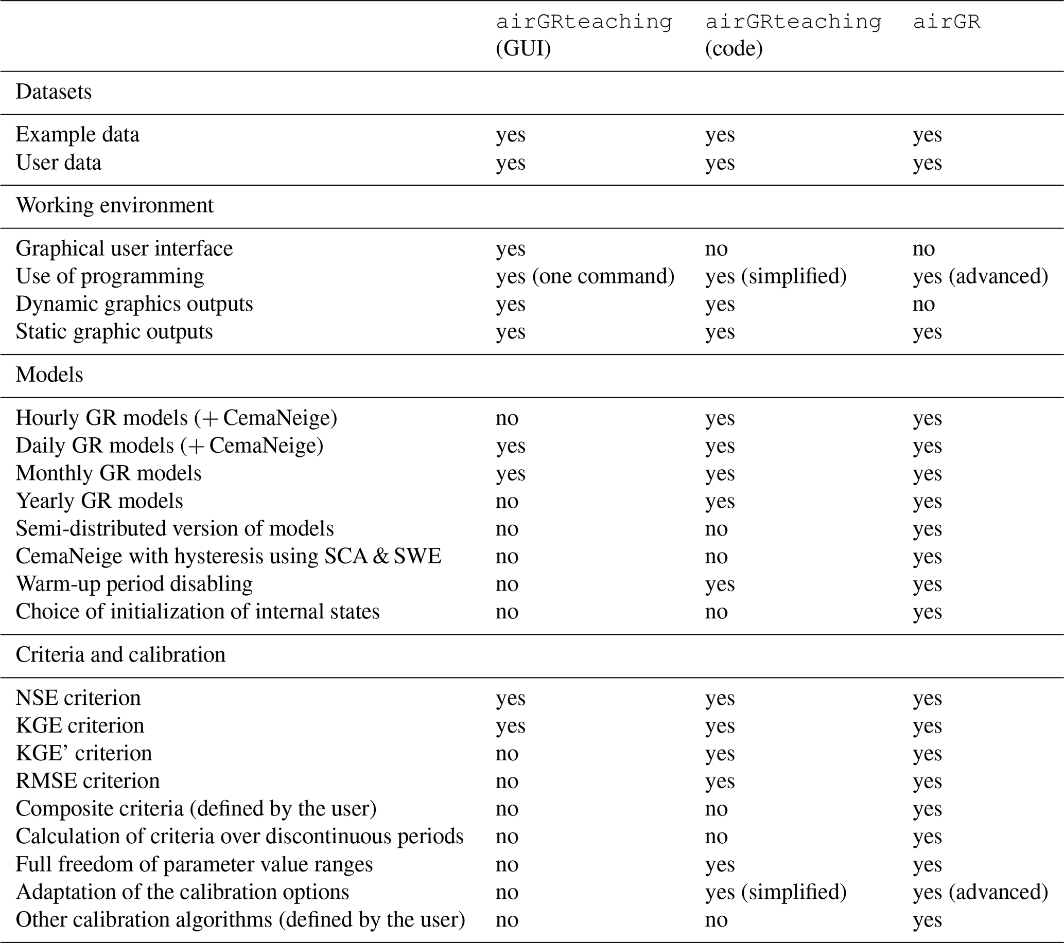
Table 1 airGR and airGRteaching features. (SCA: snow cover area; SWE: snow water equivalent; NSE: Nash–Sutcliffe efficiency, Nash and Sutcliffe, 1970; KGE: Kling–Gupta efficiency, Gupta et al., 2009; KGE': modified Kling–Gupta efficiency, Kling et al., 2012; RMSE: root-mean-square error).

2.4 airGRteaching features

airGRteaching contains only a few functions, which can be split into two groups:

1. a small set of functions to prepare data, to calibrate and run hydrological models, and to plot outputs, i.e., the basic functions needed to undertake a hydrological modeling study;

2. a function to launch a graphical user interface (GUI) to set up the hydrological models manually.

These two levels of use allow teachers to choose between different levels of technical difficulty. They can choose the most adapted use according to the time available for the exercises, the teaching objectives, and the students' skills.

To get started with the package, particular attention was given to the documentation. The user manual describes the implementation of functions precisely and succinctly and provides simple examples (https://cran.r-project.org/web/packages/airGRteaching/airGRteaching.pdf, last access: 30 December 2022). In addition, a website was created to explain how to use the different features step by step and to answer frequently asked questions (https://hydrogr.github.io/airGRteaching/, last access: 30 December 2022).

Table 1 summarizes the airGRteaching (and airGR) features.

2.4.1 Basic functions for undertaking a hydrological modeling study

The main steps required to undertake a hydrological modeling study can be performed with airGRteaching with the help of a few simple functions:

• A data preparation function, PrepGR(). With only three main arguments, namely, the hydrometeorological input data as a data frame or independent vector time series, the name of the rainfall-runoff model to run, and a Boolean indicating whether the CemaNeige snow model is activated, this function prepares all the necessary inputs in the correct format for the airGRteaching functions. If CemaNeige is activated, additional arguments are needed (e.g., catchment elevation distribution).

• A calibration function, CalGR(). With three main arguments, namely, the object produced by PrepGR(), the objective function name (i.e., which criterion is used to optimize the parameter values), and the calibration period start and end, this function calibrates the chosen GR model. If desired, a transformation of discharge can be chosen for the objective function calculation in order to give more weight to certain ranges of discharges (Santos et al., 2018), and a warm-up period can also be defined.

• A simulation function, SimGR(). With four main arguments, namely, the object produced by PrepGR(), the parameter values (output of CalGR() or defined by the user), the name of an efficiency criterion used to evaluate the simulation, and the simulation period start and end, this function runs the chosen GR model and assesses its performance. If desired, a transformation can be used for the criterion calculation, and a warm-up period can be defined.

• Static and dynamic functions, plot() and dyplot(). These functions take any of the objects produced by PrepGR(), CalGR(), and SimGR() as main arguments (to be chosen). Graph-tuning arguments are available but optional. The dynamic graphs show the observed and simulated discharge time series. The static graphs render a choice of graphs to be selected with the which argument. Dynamic graphs use the functionalities of the dygraphs package (Vanderkam et al., 2018).

Many graphical outputs are available (see Appendix A and B). Figure A1 provides a general overview of the precipitation and streamflow records to identify possible outliers and periods with missing data. Figure A2 adds the simulated streamflow to the previous graph in order to have an overall view of the calibrated model behavior and provides graphical diagnostic tools to check whether the simulated streamflow hydrograph fits the observed streamflow hydrograph. Figure A4 focuses on time series graphs (available in Fig. A2) and adds the potential evapotranspiration. Figure A3 focuses on the errors of the model compared to the observed streamflows. Figure A5 helps the concept of parameter optimization to be understood by displaying the tested parameter values and the correspondence with the value of the criterion chosen as objective function. In general, dynamic graphs (Figs. B1 and B2) help the values of time series to be read more precisely and to zoom in on a particular event for each of the two axes (some options are available, e.g., to add a rolling average or a time range selector).

2.4.2 The graphical user interface

Using the functionalities of the shiny package (Chang et al., 2022), the airGRteaching graphical user interface (GUI) called with the ShinyGR() function allows one to use the GR models with no programming skills at all, thanks to an intuitive interface. The ShinyGR() function takes hydrometeorological data and the simulation period start and end as arguments. Additional arguments can be provided if snow is present. Data can be provided for several catchments, and the function offers the possibility to use different themes for the interface. The GR and CemaNeige models and the objective function are to be selected within the interface.

Figure 1 presents a commented example of the interface. Several intuitive elements can be found. On the left side are the following:

• “Choose a dataset” enables a dataset to be selected from those provided by the user to the function.

• “Choose a model” enables a model to be selected among the GR2M monthly model and the GR4J, GR5J, and GR6J daily models according to the time step of the datasets provided (models at other time steps are not included in the GUI) and to activate the CemaNeige snow accumulation and melt model for the daily models.

• “Parameter values” enables the parameters of the models to be modified. The parameters proposed are automatically adapted to the chosen model and the ranges are predefined. Changing any parameter value causes a real-time update of the plots and displayed scores (see below).

• “Automatic calibration” enables an automatic calibration to be performed by optimizing a chosen objective function (among the Nash–Sutcliffe efficiency (NSE) and the Kling–Gupta efficiency (KGE) and with a squared root, inverse, or no transformation of discharge).

Figure 1 Overview of the airGRteaching GUI and identification of its main elements.

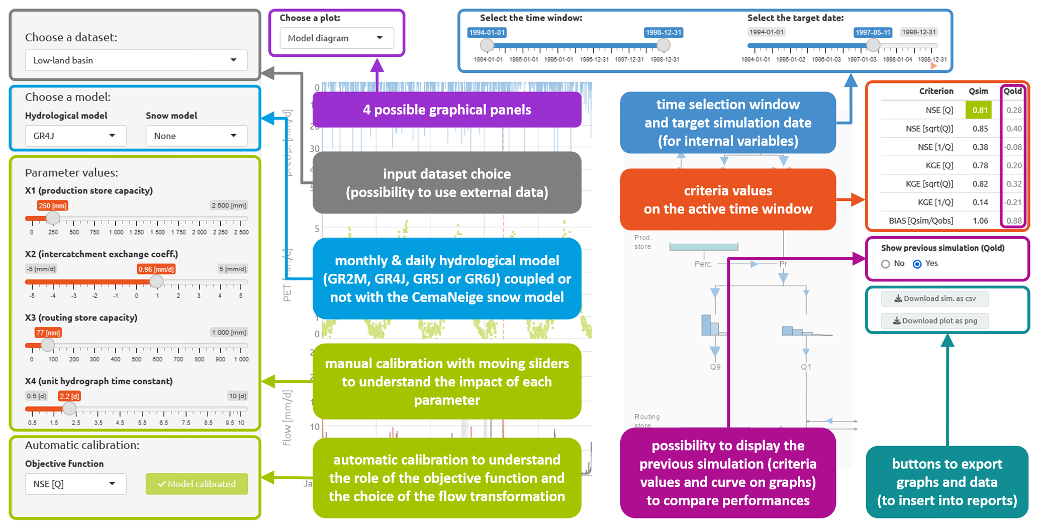
The following options are at the top:

• “Choose a plot” enables the kind of plot that is displayed to be changed (see Fig. 2). Users can choose from the following.

  • “Flow time series” are dynamic plots of observed and simulated discharge as well as precipitation time series and discharge errors.

  • “Model performance” is an ensemble of static plots of observed and simulated discharge as well as precipitation time series and of annual regimes, flow duration curves, and a scatter plot between simulated and observed discharges.

  • “State variables” are dynamic plots that show the time series of GR model store levels as well as the time series of internal model fluxes.

  • “Model diagram” is a plot that can be dynamic and on the right shows the scheme of the chosen GR model and the dynamic evolution of all its fluxes with time and the related hydrometeorological data.

• “Select the time window” enables the user to zoom within the provided data period or to move the window using the sliders.

• “Select the target date” enables a specific date to be targeted (only for the “Model diagram” panel).

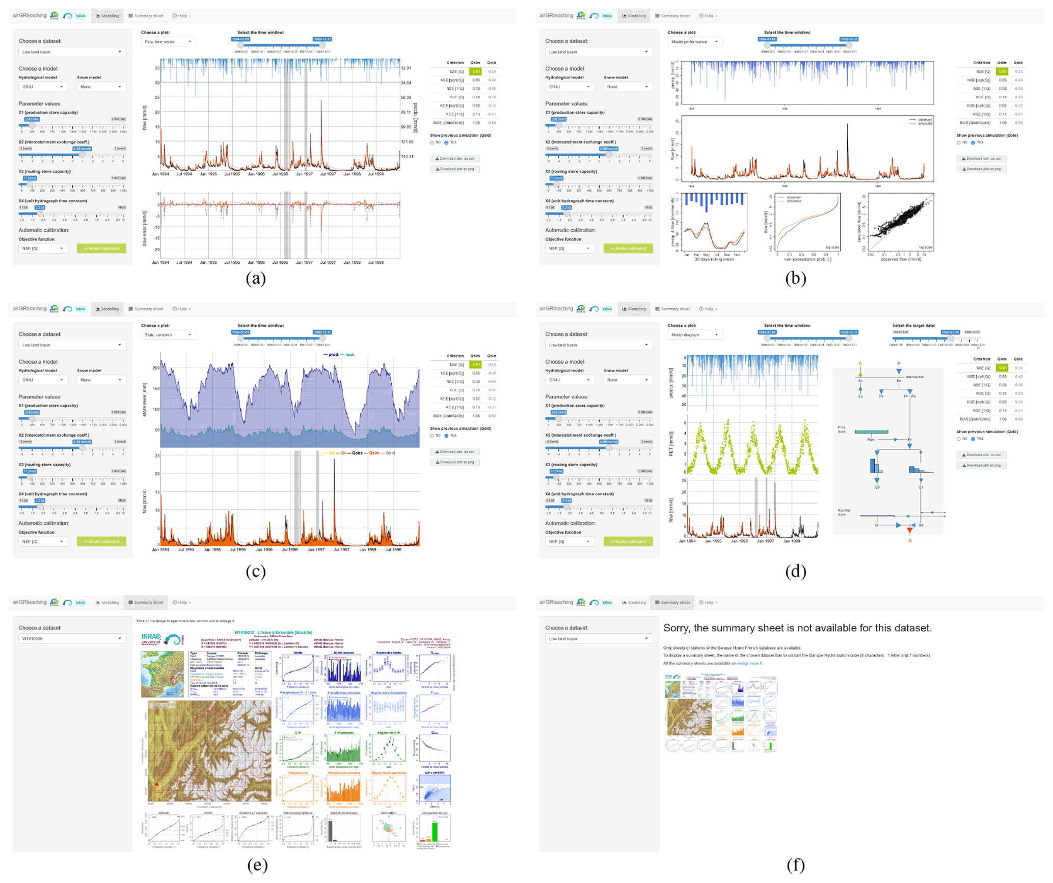
Figure 2 airGRteaching GUI “Modeling” panels (a–d) and “Summary sheet” panels (e, f) that can be reached through diverse clicking. In the following, the center column of the GUI is described for each possible panel; all other elements of the GUI were described in Fig. 1. (a) “Flow time series”: precipitation, observed, and simulated hydrographs (top) and flow error time series (bottom). (b) “Model performance”: precipitation (top), observed and simulated hydrographs (middle), simulated and observed regime hydrographs (bottom left), flow duration curves (bottom center), and a scatter plot between simulated and observed discharges (bottom right). (c) “State variables”: time series of reservoir levels (top) and runoff components (bottom). (d) “Model diagram”: time series (left) of precipitation, potential evapotranspiration, and simulated and observed flows (from top to bottom) and interactive model diagram (right; with updating of the flows, the size, and the level of the reservoirs). (e) Hydrometeorological and topographical characteristics of the selected catchment (Brigode et al., 2020, only available for French catchments). (f) Same as (e) when the catchment characteristics are not available.

In the center, the plots are proposed by the “Choose a plot” panel.

On the right, the following are found:

• A table of criteria provides the values of seven performance criteria (NSE and KGE with use of squared root, inverse, or no transformation of discharge, in addition to the bias).

• Using the “Show previous simulation Qold” option, the previously obtained simulated time series appear on the plots provided in the center of the GUI as a dotted gray line. In addition, ticking this option makes criteria of this previous simulation appear in the criteria table introduced above. This option has no effect on the “Model performance” panel.

• Two buttons allow users to download the displayed plot in a PNG file format, which can be useful for a report for example (in order to ensure the tracking of the downloaded files, various information is automatically added to the file header: name of the dataset, name of the model, simulation period, and parameter values; see Appendix C), and the hydrometeorological data (including the simulation) in a CSV file format, to be used externally for further analysis or to be saved.

Figure 2 presents the airGRteaching GUI “Modeling” panels (a–d) and “Summary sheet” panels (e–f).

If R is not installed on the students' computers, it is possible to run the airGRteaching GUI online. Indeed, the graphical user interface is available at https://sunshine.inrae.fr/app/airGRteaching (last access: 20 July 2023) with demo datasets.

2.4.3 Data associated with airGRteaching

Users are free to use their own datasets, but the airGRteaching package benefits from the airGRdatasets package (Delaigue et al., 2023a), which contains a dataset of 19 different catchments located in France (Fig. 3 and Table 2). This dataset is a subset of the larger CAMELS-FR dataset (Delaigue et al., 2022) and has been assembled to include various French hydro-climatic regimes, with 12 rain-dominated catchments, 1 rain- and snow-dominated catchment, 2 snow-dominated catchments, 2 Mediterranean catchments, and 2 groundwater-dominated catchments. Figure 4 shows the main characteristics of the catchment set. Catchment area ranges from 25 to 3917 km², with half of the catchment set draining less than 686 km².

Table 2 List of the 19 catchments in France included in the airGRdatasets package (ID: identification letters displayed in Fig. 3).

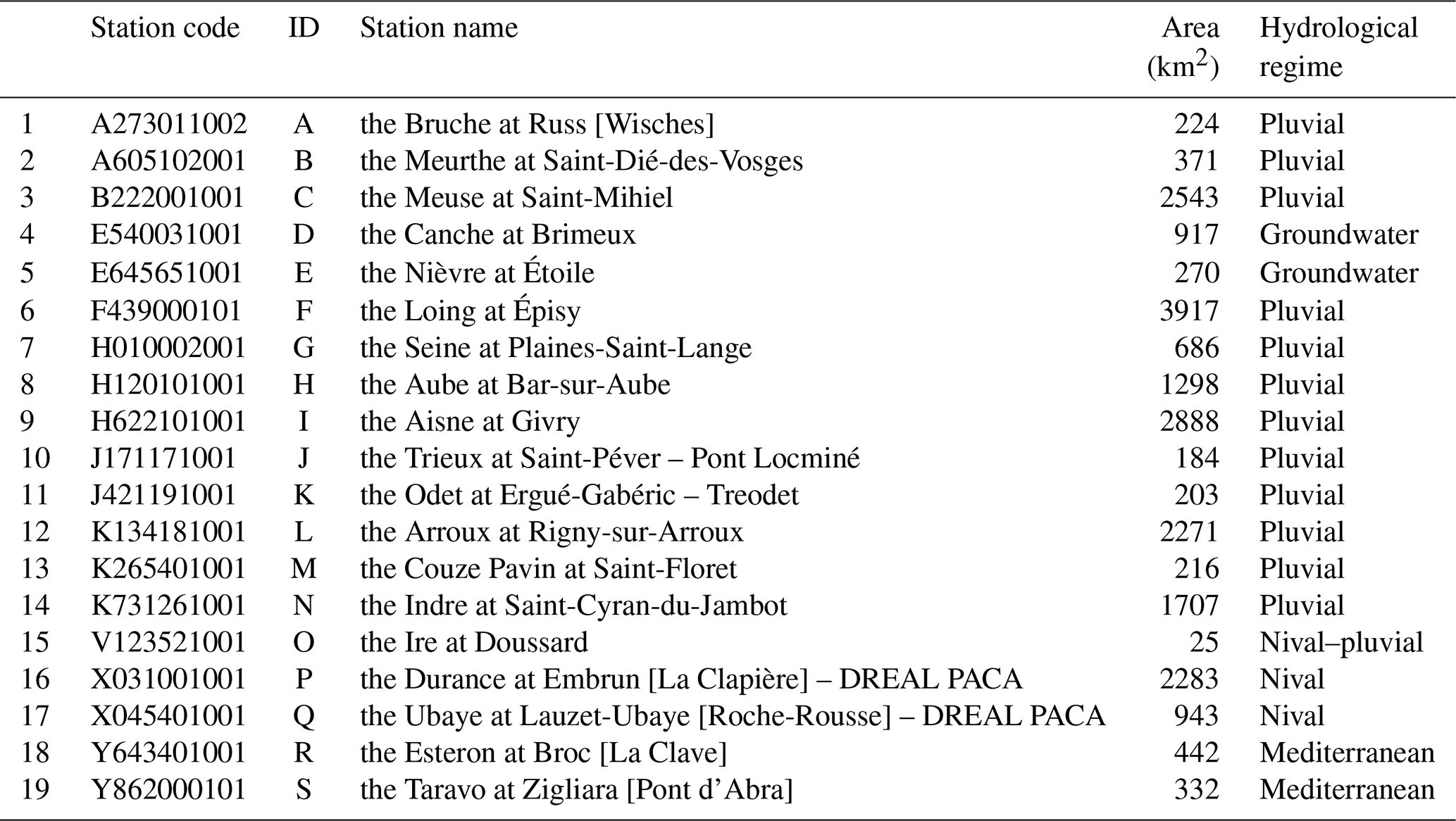
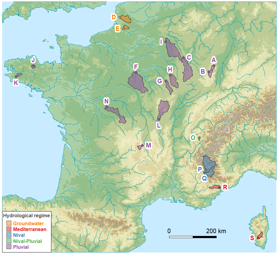
Figure 3 Location of the 19 catchments in France included in the airGRdatasets package (map from the airGRdatasets package documentation: Delaigue et al., 2023a; using hydrometric station coordinates and catchment boundaries: Delaigue et al., 2022; river network: Lehner and Grill, 2013); DEM: GEBCO Bathymetric Compilation Group, 2021.

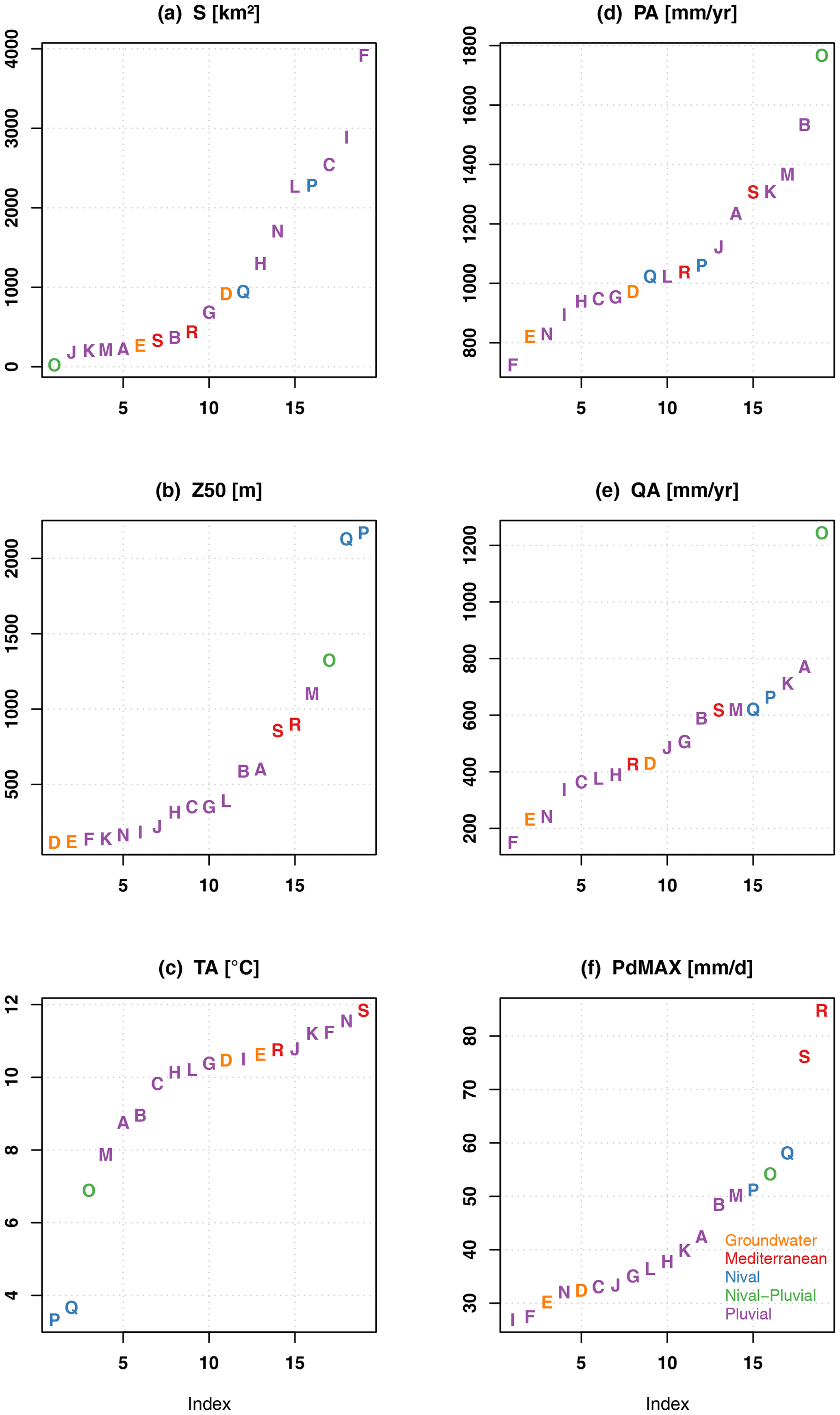
Figure 4 Distribution of the characteristics of the 19 catchments included in the airGRdatasets package. (a) “S”, area (km²); (b) “Z50”, median altitude (m a.s.l.); (c) “TA”, median of the mean annual air temperature (^∘C); (d) “PA”, median of the annual precipitation (mm yr⁻¹); (e) “QA”, median of the annual flow (mm yr⁻¹); and (f) “PdMAX”, median of the maximum annual daily precipitation (mm/day), versus the catchment indexes. The statistics have been calculated over the available daily time series in the airGRdatasets package (i.e., from 1 January 1999 to 31 December 2018; only the years with less than 10 % of missing streamflow values have been considered).

The dataset is composed of both static geomatic and physiographic catchment indices and hydro-climatic time series (solid and liquid precipitation, potential evapotranspiration, air temperature, and streamflow time series). The climatic time series have been extracted from the SAFRAN reanalysis (Vidal et al., 2010) and aggregated at the catchment scale, while streamflow series have been extracted using the HydroPortail (https://hydro.eaufrance.fr/, last access: 30 December 2022). These hydro-climatic temporal series are available at the daily time step.

3 Teaching hydrology with airGRteaching

This section and the accompanying sections in the Appendix present tests based on the airGRteaching package and designed to illustrate rainfall-runoff modeling, model calibration, evaluation, and robustness in hydrological classes. These tests are also available as a vignette in the airGRteaching package: users can thus recreate all these illustrations using their own datasets.

3.1 Understanding rainfall-runoff modeling

3.1.1 The role of model components and parameters

Rainfall-runoff models are composed of different components, e.g., reservoirs or unit hydrographs, whose behavior is defined by equations and parameters. Parameter estimation is a key step toward tailoring the models to a specific catchment. Understanding the role of model components and parameters is therefore an unavoidable preliminary step to performing hydrological modeling.

To illustrate the production and the routing parts of hydrological modeling that are present in any model, it is possible to use the different GR models included in airGRteaching and to produce rainfall-runoff transformations considering different model parameter values.

The GR4J model (Perrin et al., 2003) comprises a production store (X1 parameter), which determines the actual evapotranspiration and the net rainfall (see Appendix C4 for a GR4J flowchart). The routing of net rainfall is determined through two unit hydrographs (X4 parameter) and a routing store (X3 parameter). A final component, representing the intercatchment groundwater exchange, is determined by the X2 parameter.

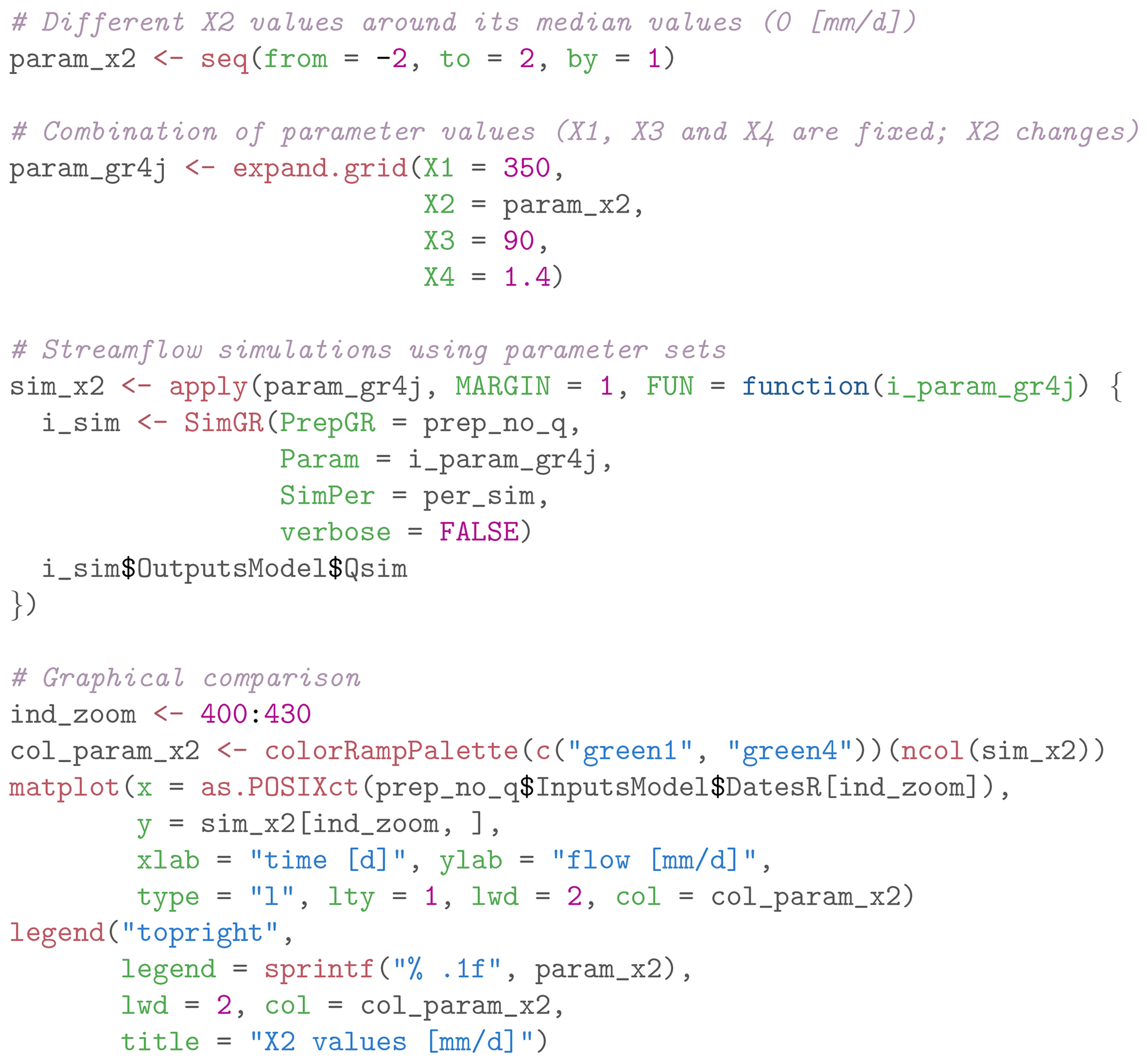
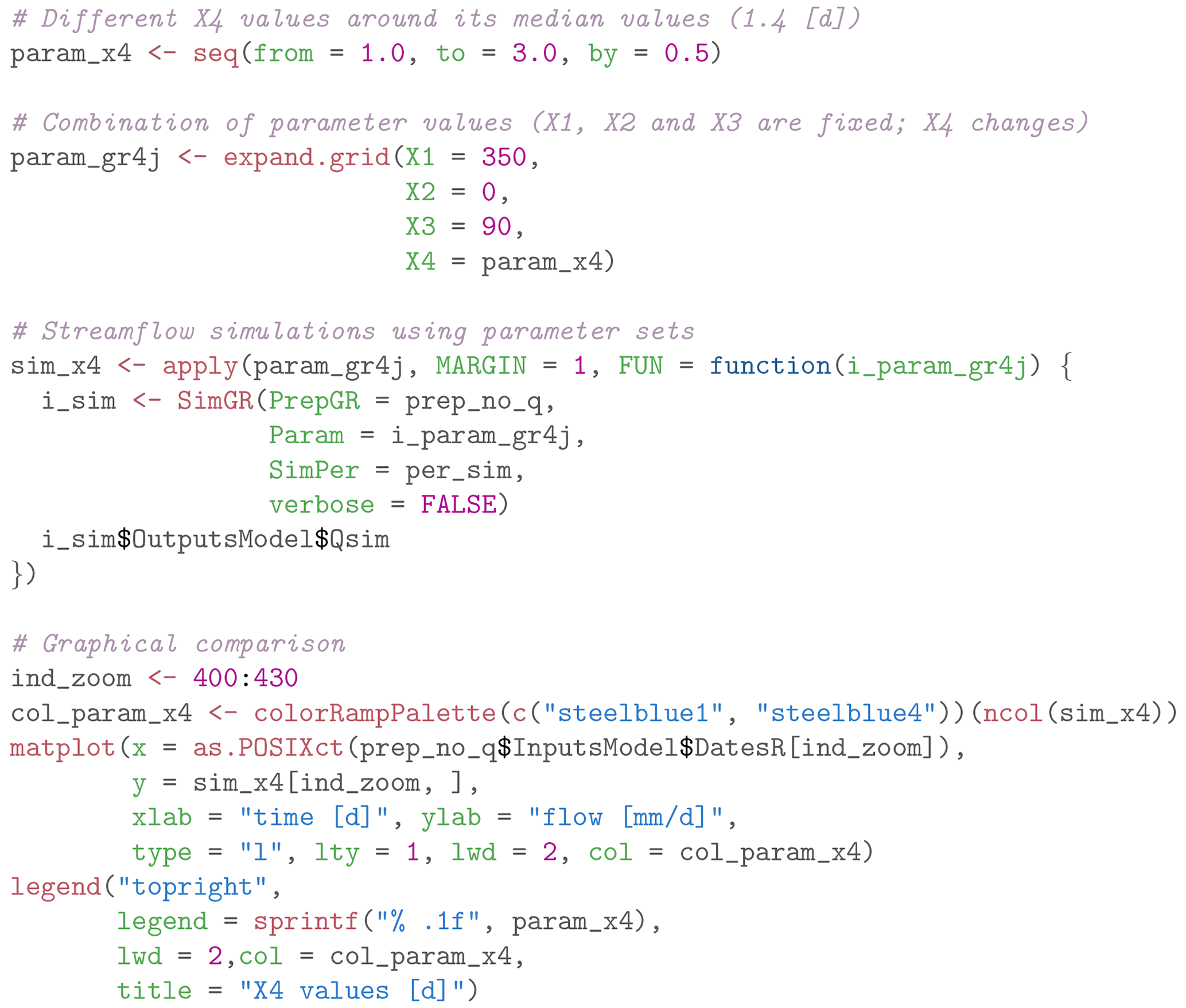
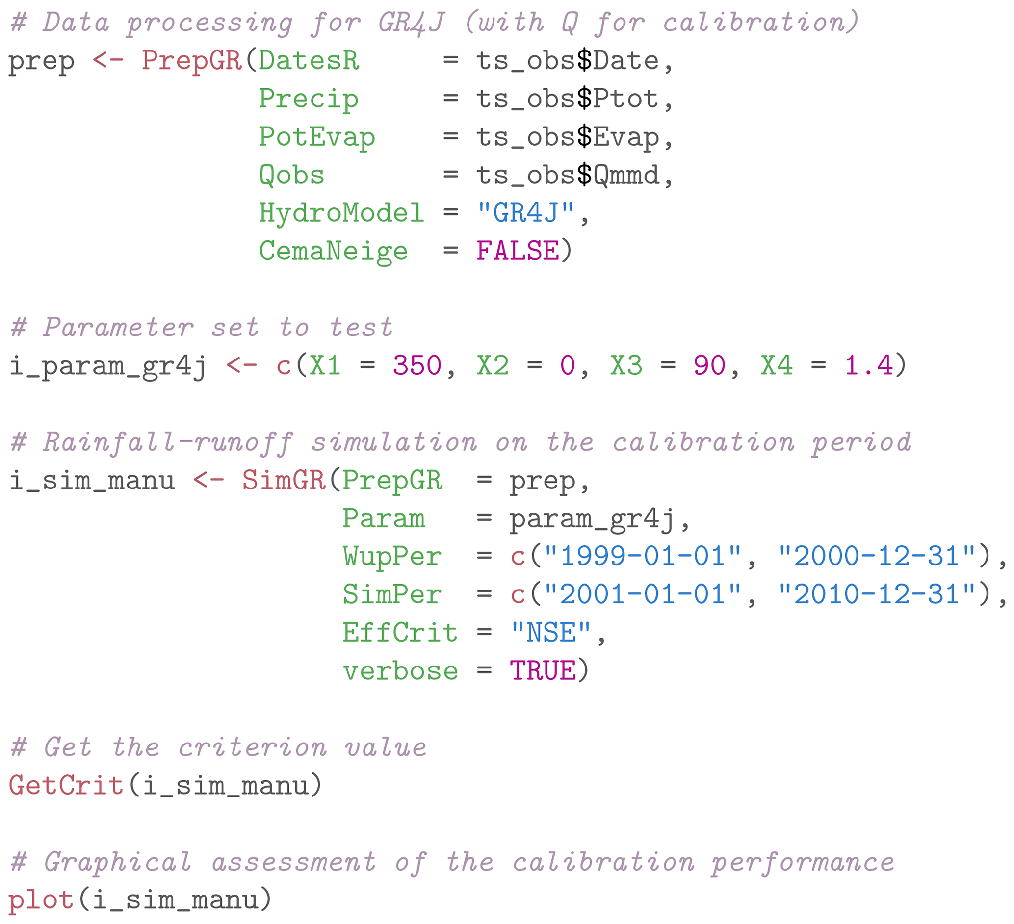
As an example, the command lines in Appendix Listing D1 and Fig. 5 illustrate the role of the X2 parameter in the production part of the rainfall-runoff transformation, showing higher streamflow values simulated with higher X2 values, since higher X2 parameter values lead to more positive incoming water from groundwater. Moreover, Fig. 6 illustrates the role of the X4 parameter in the routing part of the rainfall-runoff transformation, with delayed flood peak values when considering higher X4 values (see command lines in Appendix Listing D2).

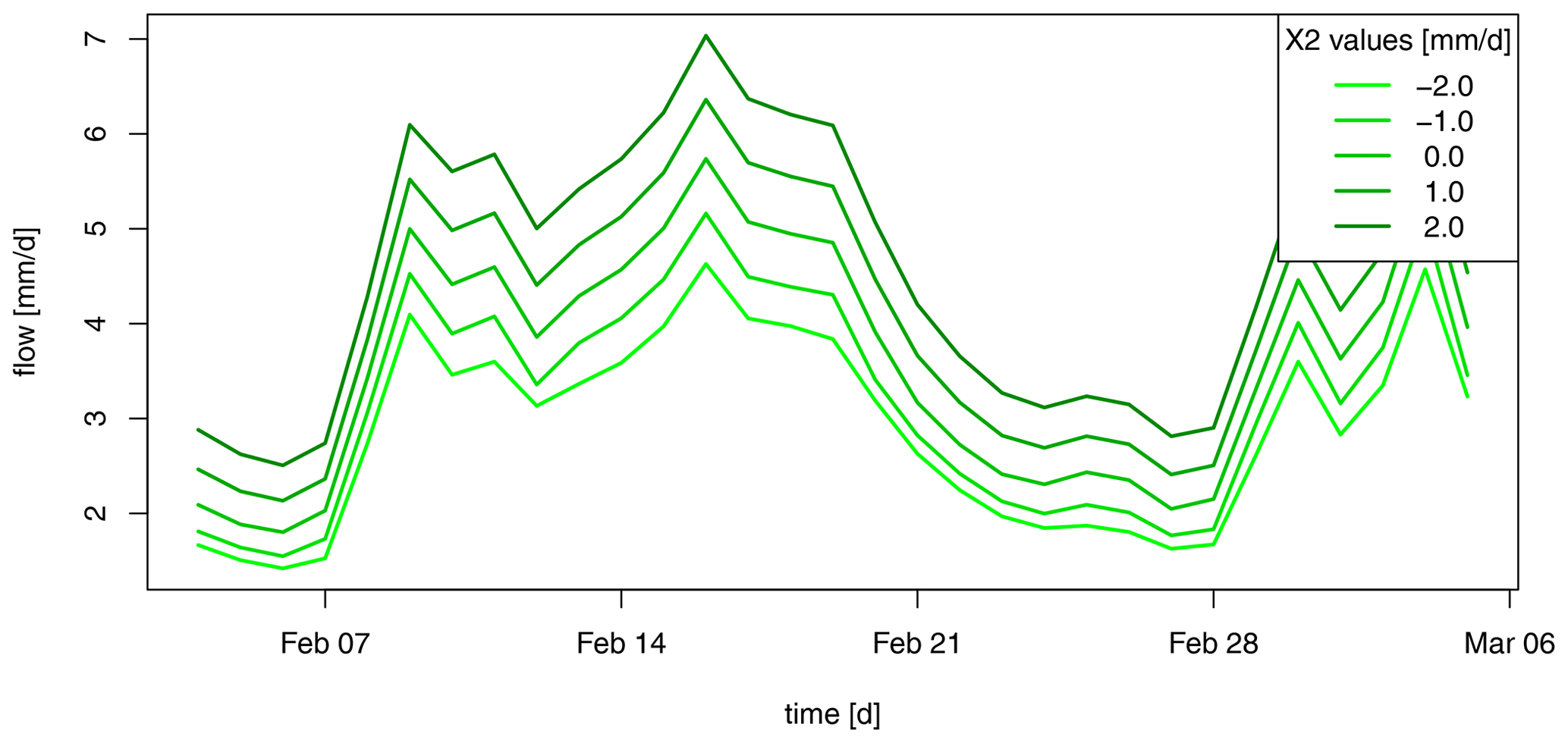
Figure 5 The role of the production component in GR4J illustrated by an example of flow simulation sensitivity to the X2 parameter values (groundwater exchange coefficient, mm d⁻¹).

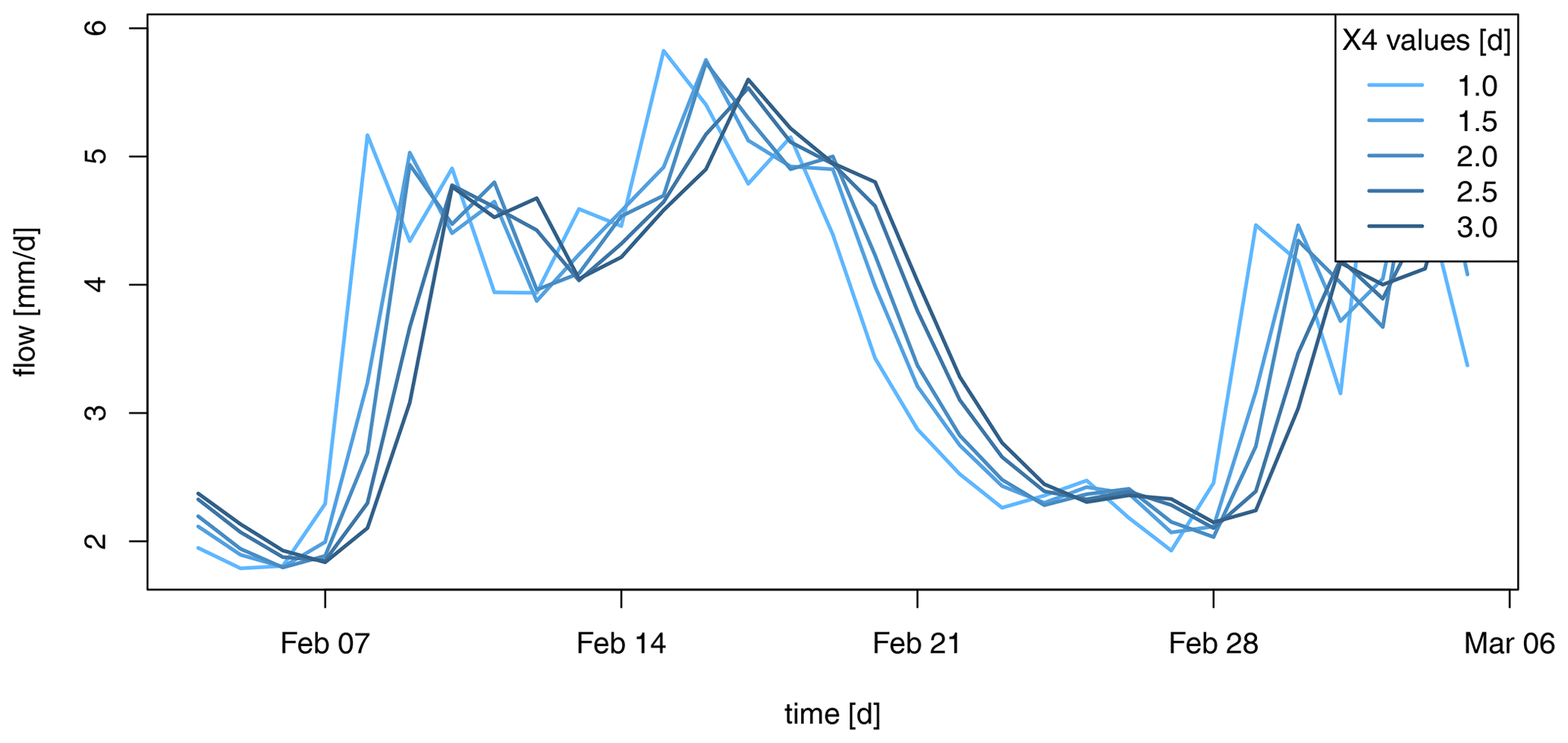
Figure 6 The role of the routing component in GR4J illustrated by an example of flow simulation sensitivity to the X4 parameter values (time base of unit hydrographs, in days).

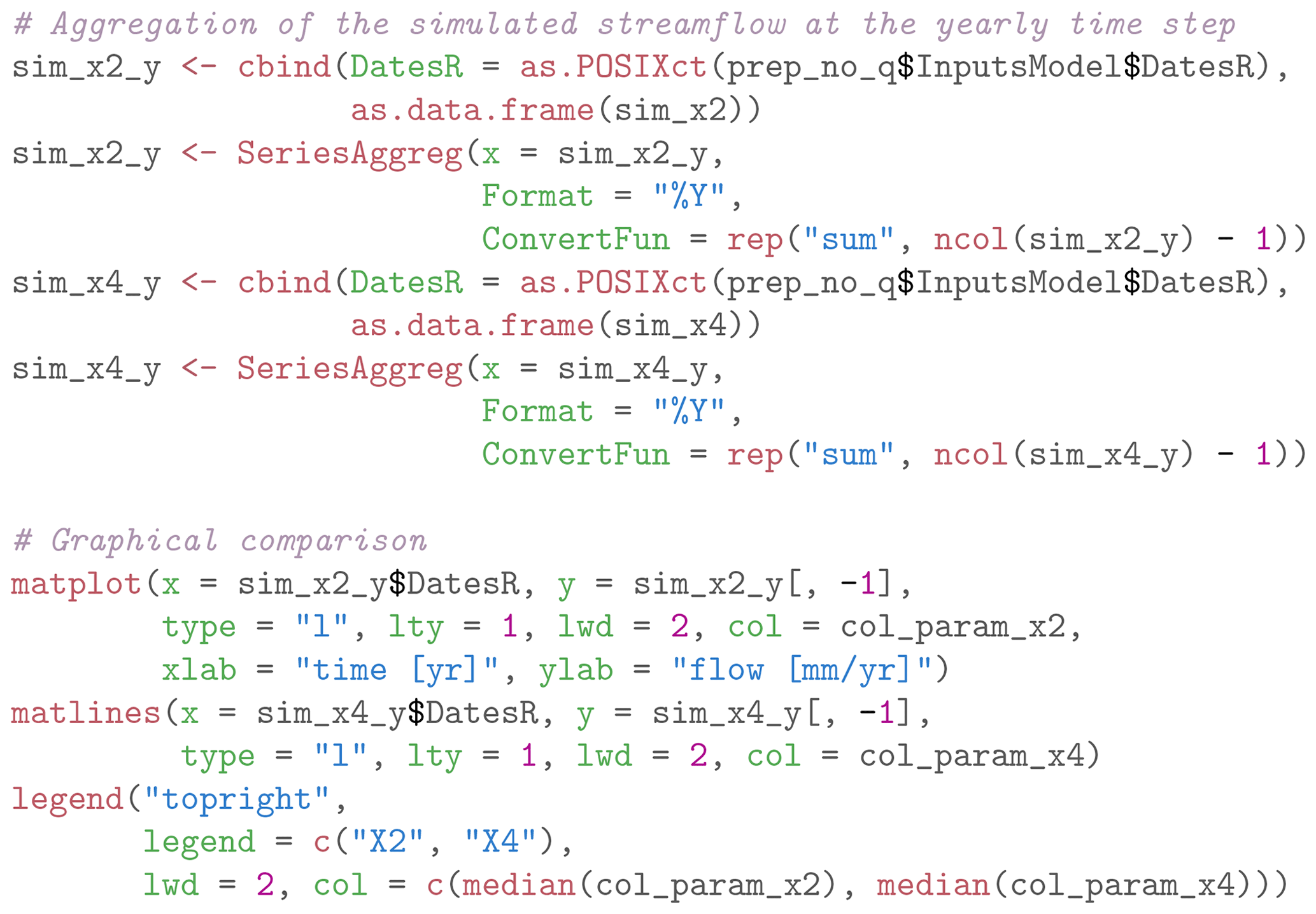
The relative importance of the production and routing functions depends on the time step considered for the rainfall-runoff simulation. The production process is more important for the larger time steps (e.g., month or year) since it controls the catchment water balance. This can be easily illustrated by aggregating simulations performed at a daily time step to a yearly time step (see command lines in Appendix Listing D3). Figure 7 compares, at the annual time step, the GR4J daily simulations performed using different X2 parameter values with the simulations performed using different X4 parameter sets. We can observe that at the annual time step, the impact of considering different X4 parameter values is limited compared to the use of different X2 parameter values.

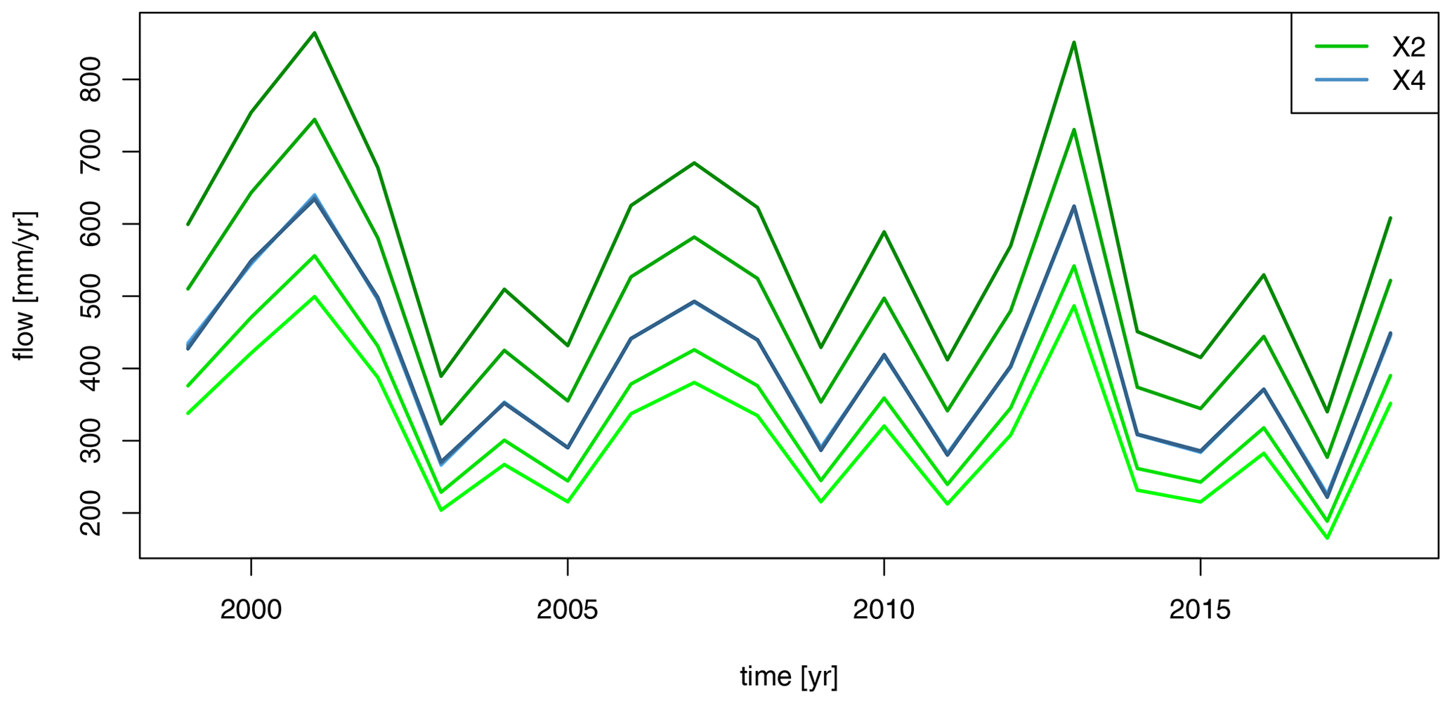
Figure 7 Comparison, at the annual time step, between GR4J daily simulations performed with different X2 parameter values (in green gradient) and simulations performed with different X4 parameter sets (in blue gradient).

3.1.2 On the need to perform a model warm-up

Initial values of the model water storage must be specified at the beginning of a simulation. The way initial levels are defined can lead to potentially significant model errors. The most convenient way for modelers to initialize rainfall-runoff models is to perform a warm-up run of the model in order to limit the impact of this unknown.

This issue can be illustrated with airGRteaching by considering different warm-up period lengths (see command lines in Appendix Listing D4). Figure 8 illustrates a portion of the streamflow simulations obtained considering (i) no warm-up period, (ii) a 1-month warm-up period, and (iii) a 1-year warm-up period of the two GR4J stores. Figure 8 shows that the three simulations converge after a bit more than 5 months, reinforcing the necessity of performing a sufficiently long warm-up. Please note that by default, airGRteaching initializes the production and the routing stores at 30 % and 50 % of their capacity, respectively.

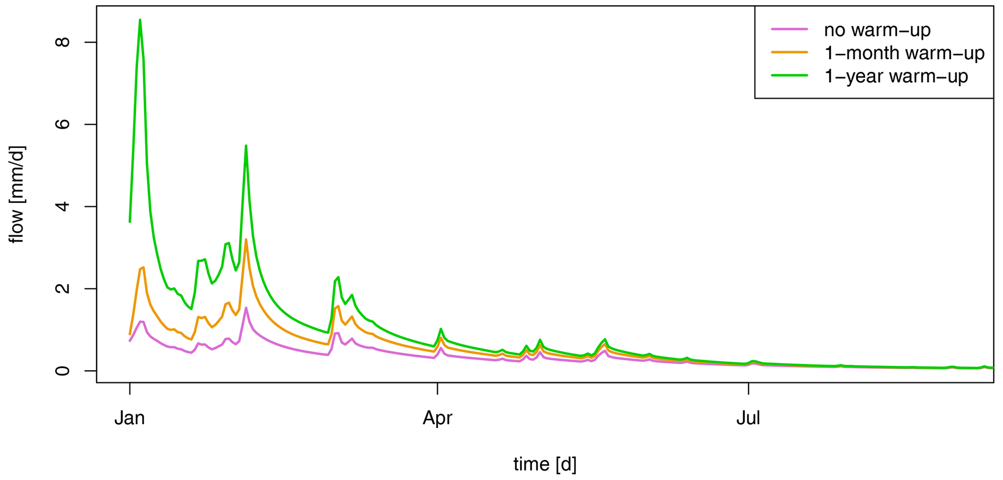
Figure 8 Example of streamflow simulations obtained considering no warm-up period (in purple), a 1-month warm-up period (in orange), and a 1-year warm-up period (in green) of the GR4J two stores.

3.2 Model calibration, evaluation, and robustness

3.2.1 Manual calibration

In the airGRteaching GUI (see Fig. 2), it is possible to test different parameter sets of the GR rainfall-runoff models and to estimate the performance of each tested parameter set in order to perform a manual calibration. A classic way to do so through the airGRteaching GUI is to select a criterion as an objective function in the table showing the criteria values on the right, to activate the “Show previous simulations (Qold)”, and to modify parameter values step by step until the simulation and criterion are satisfactory. This can also be done using the simple command-line functions (PrepGR() and SimGR(); see command lines in Appendix Listing D5).

3.2.2 Automatic calibration

Automatic calibration of model parameters is also possible in airGRteaching using the procedure described by Michel (1991) and by considering one objective function such as NSE or KGE. To do so, there are two options in airGRteaching:

1. clicking on the automatic calibration button in the airGRteaching GUI;

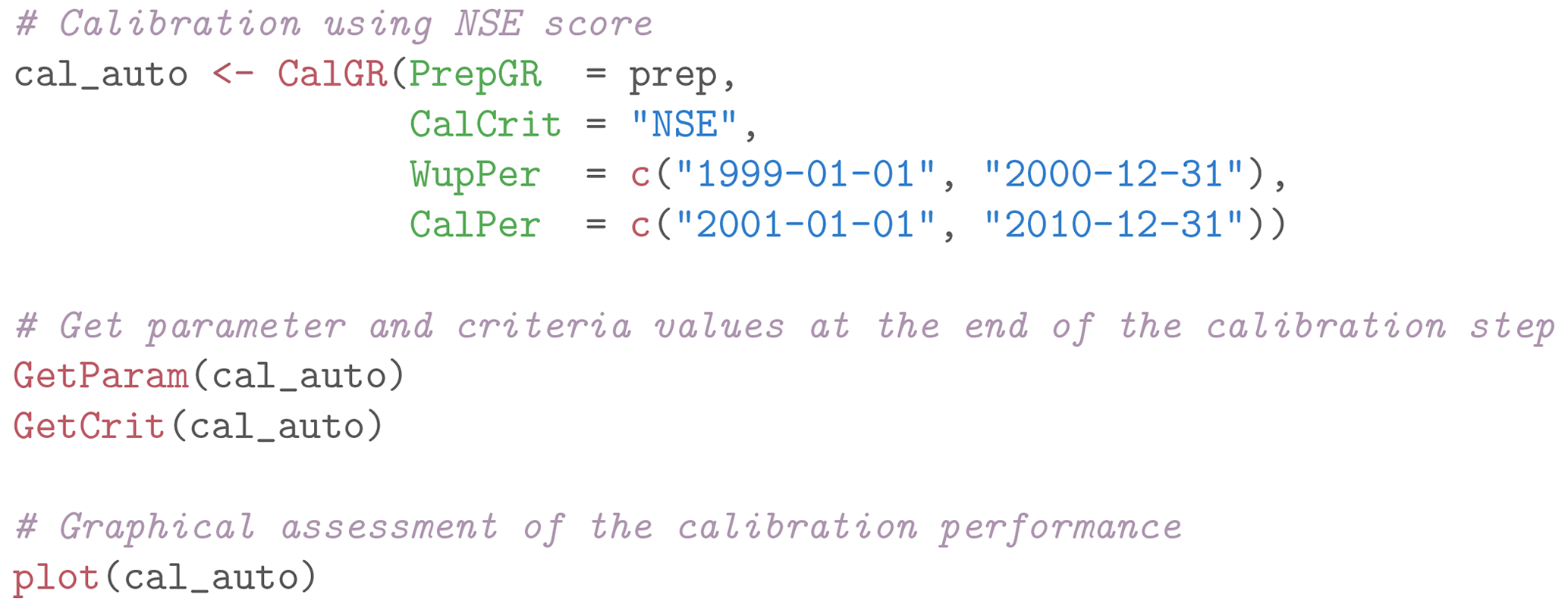
2. using the simple airGRteaching command-line functions (PrepGR() and CalGR(); see command lines in Appendix Listing D6).

The calibration algorithm available in airGRteaching comes from airGR and is described in further detail in Coron et al. (2017, Sect. 2.3). Two distinct steps are included in the procedure:

1. A systematic inspection of the parameter space is performed to determine the most likely zone of convergence. This is done either by direct grid screening or by constrained sampling based on empirical parameter databases.

2. From the best parameter set of the previous step, a steepest-descent local search procedure is carried out to find an estimate of the optimum parameter set.

airGRteaching allows the second step of this procedure to be visualized (see command lines in Appendix Fig. A5).

3.2.3 How to evaluate model calibration

Different ways to evaluate the model calibration performance may be conceived using airGRteaching: evaluating criteria on the calibration period, examining the graphical summary of the calibration performance (airGR::plot()), and comparing simulated and observed streamflow temporal series, etc.

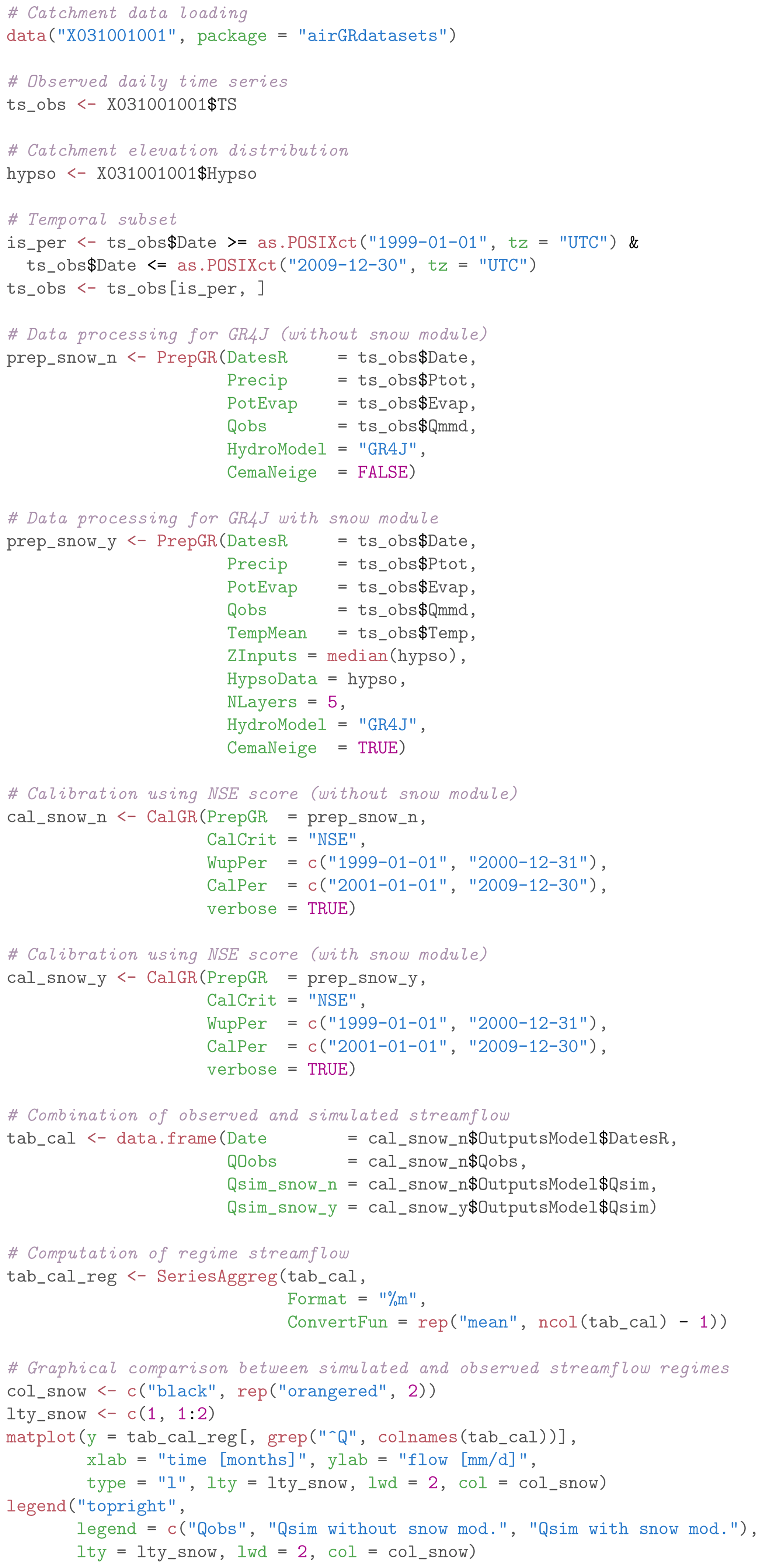
Analyzing simulated versus observed flow regimes is an informative indicator of model performance (see command lines in Appendix Listing D7). Figure 9 compares regimes in a mountainous catchment (located in the French Alps), while the flow simulation has been obtained with and without taking into account snow accumulation and melt. The regime comparison might be compelling for the students, hopefully leading them to use an additional snow accumulation and melt routine (such as CemaNeige, Valéry et al., 2014, available in airGRteaching).

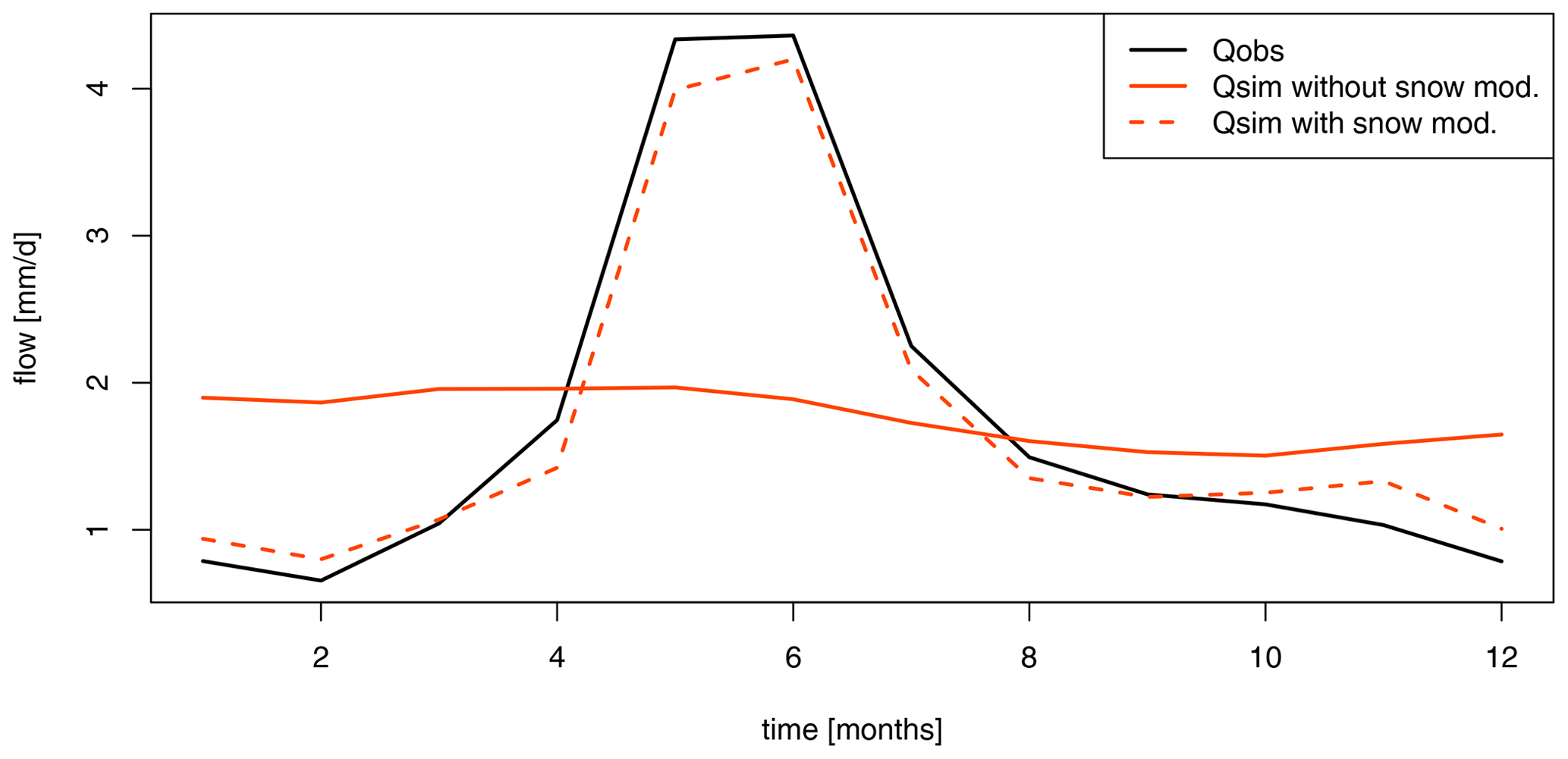
Figure 9 Example of flow regimes observed for a catchment located in the French Alps (in black) and flow regimes simulated by GR4J without considering snow accumulation and melting (solid red line) or when a snow accumulation and melting routine is used (dashed red line).

3.2.4 Objective functions for model calibration

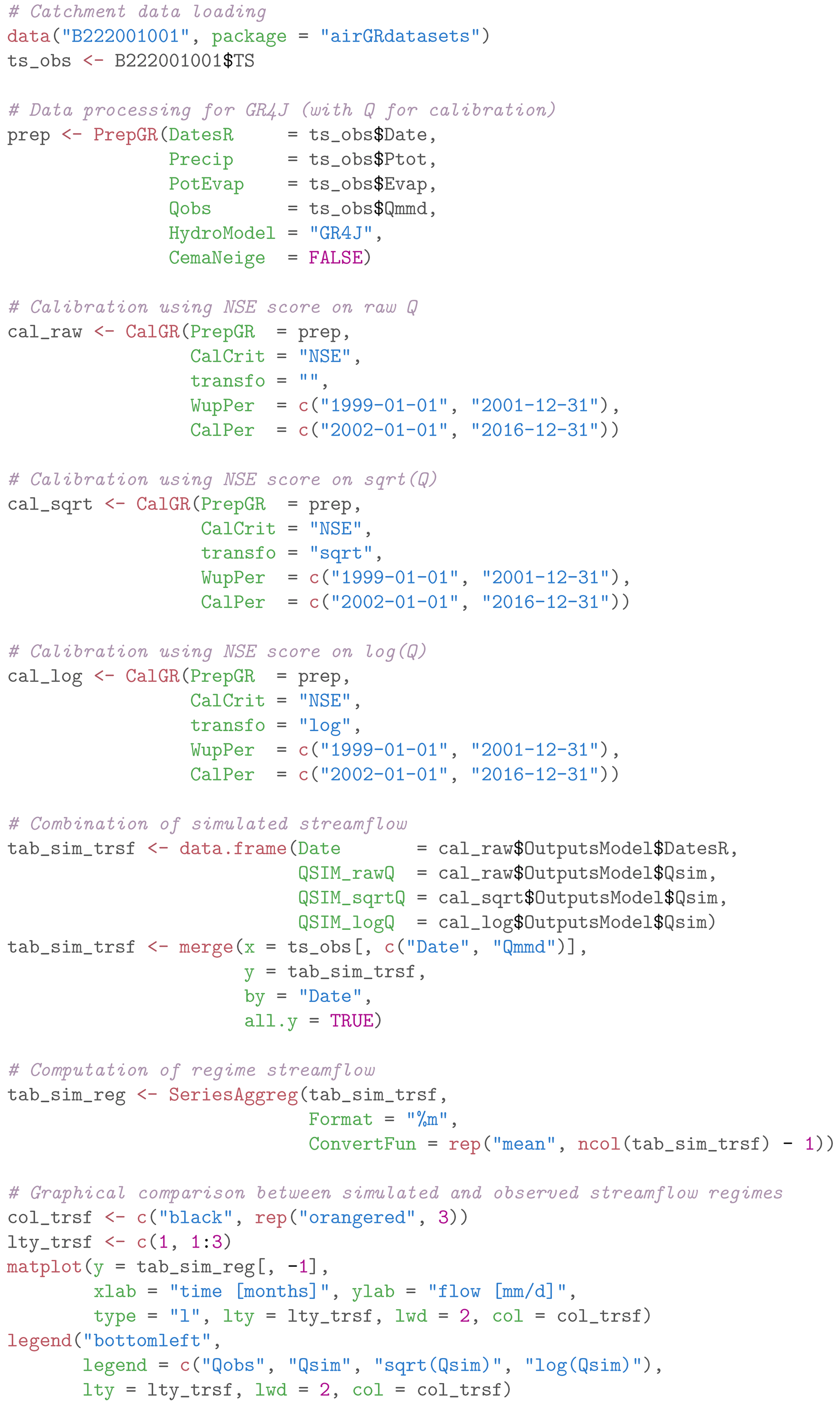
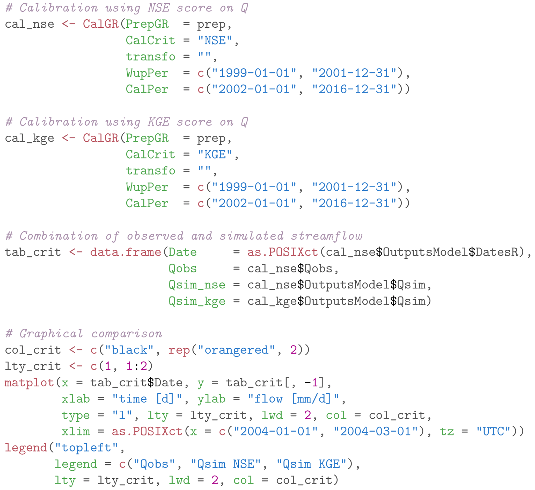
Oudin et al. (2006) and other authors showed the impact of using flow transformation in objective functions used for model calibration. It is possible, in airGRteaching, to apply different flow transformations to the objective function used for model parameter calibration (see command lines in Appendix Listing D8). Figure 10 compares the simulations performed considering GR4J parameter sets obtained after a calibration on (i) NSE calculated on natural flows (denoted as NSE_Q hereafter), (ii) NSE calculated on square-root-transformed flows (denoted as NSE${}_{\sqrt{Q}}$ hereafter), and (iii) NSE calculated on logarithmic-transformed flows (denoted as NSE_log Q hereafter), emphasizing performance in high, mean, and low flows, respectively. Logically, we can observe that the model calibrated on NSE_Q performs better for high-flow periods, and the model calibrated on NSE_log Q performs better for low-flow periods, while the model calibrated on NSE${}_{\sqrt{Q}}$ performs in between.

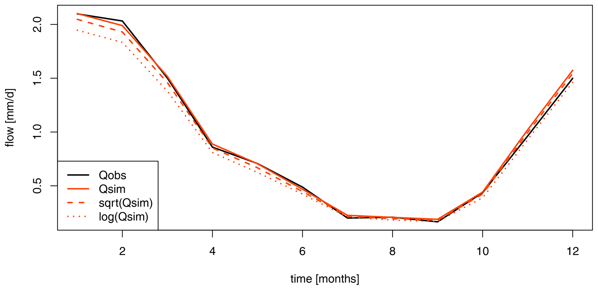
Figure 10 Example of observed flow regimes (in black) and flow simulations obtained when GR4J is calibrated on NSE calculated on untransformed flows (solid red line), NSE calculated on square-root-transformed flows (dashed red line), and NSE calculated on logarithmic-transformed flows (dotted red line).

Similarly to the use of different flow transformations during model calibration, the airGRteaching CalGR() function allows us to test several objective functions such as NSE or KGE (see command lines in Appendix Listing D9).

3.2.5 Model evaluation and robustness

Split-sample tests, i.e., calibrating and evaluating a model on non-overlapping periods (Klemeš, 1986), is key for the assessment of model transferability in time, since in practice models are used outside their calibration conditions. Split-sample tests can be performed for model calibration and evaluation using both CalGR() and SimGR() airGRteaching functions, respectively (see command lines in Appendix Listing D10).

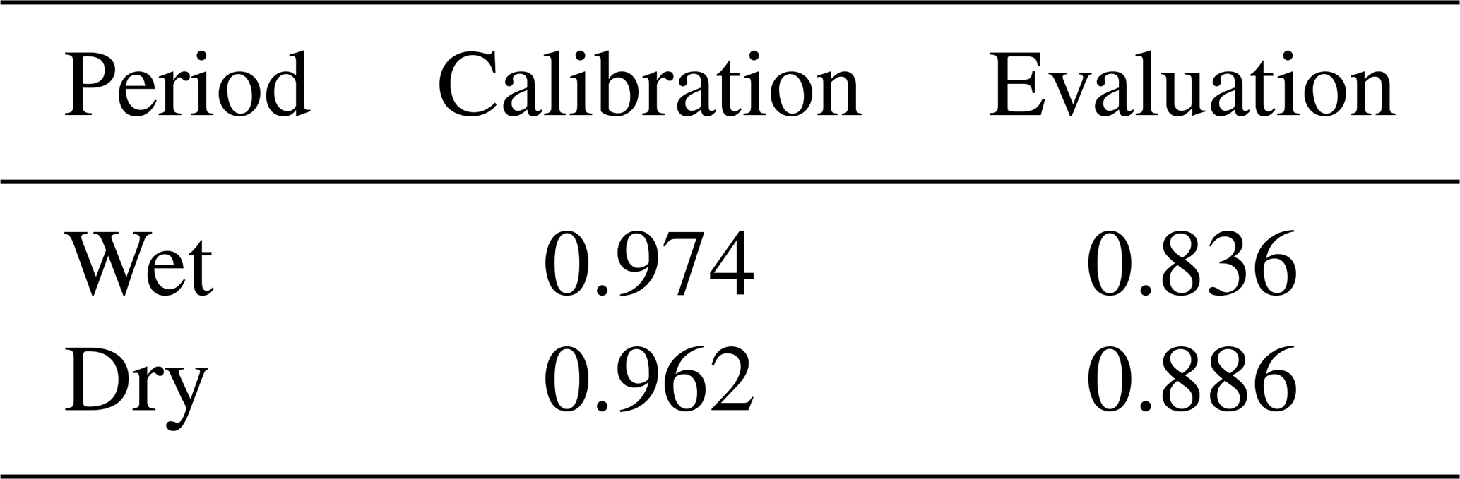
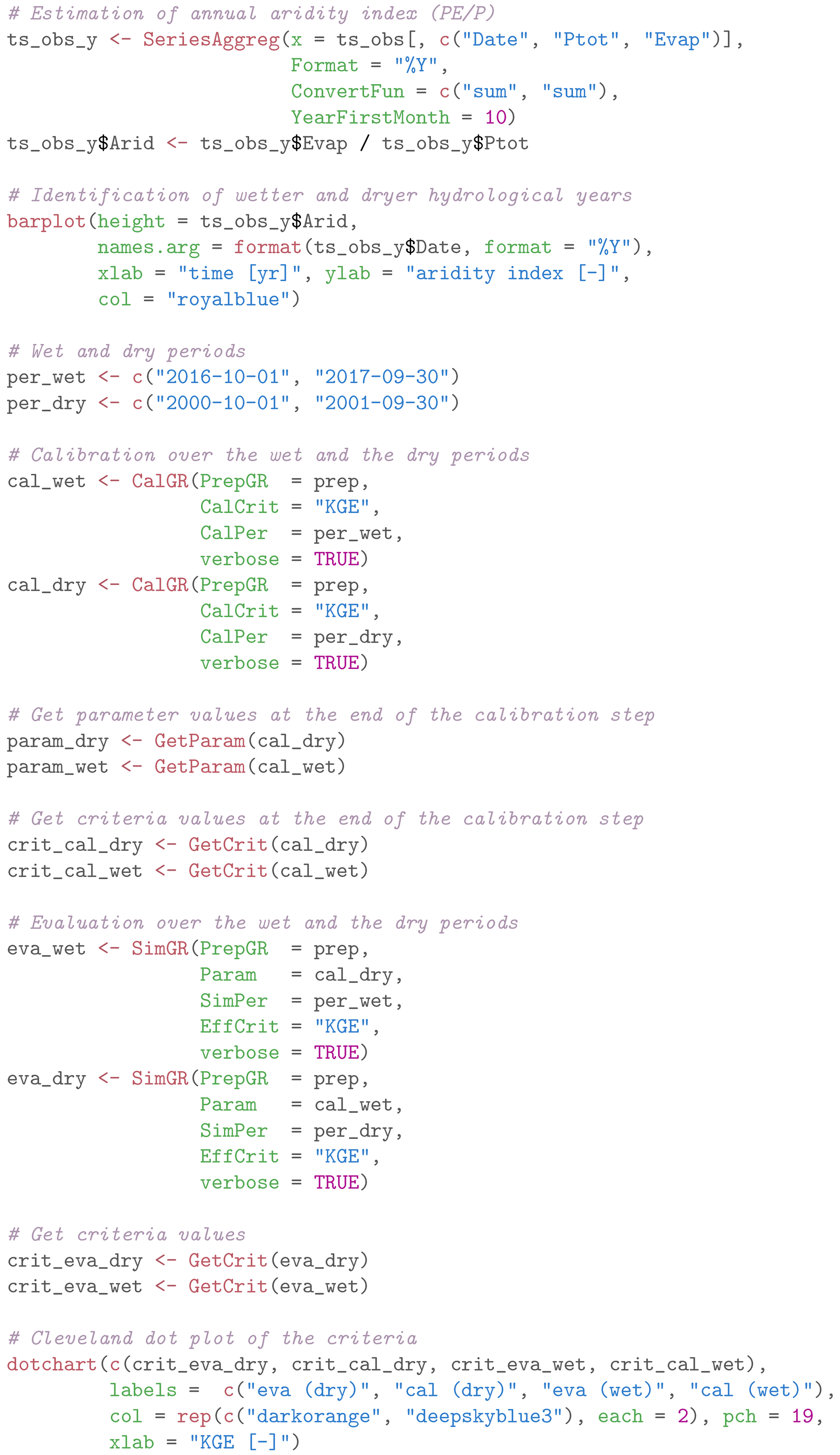
The differential split-sample test, also introduced by Klemeš (1986), consists in identifying two climatically contrasted periods in the available record and performing the split-sample test using these two periods. Table 3 presents the calibration and evaluation performance of the GR4J model obtained for two sub-periods, composed of the wettest and the driest hydrological years (based on the aridity index, i.e., the total annual precipitation divided by the total annual potential evapotranspiration; see command lines in Appendix Listing D11).

Table 3 Example of differential split-sample results (KGE score) obtained for a given catchment.

4 One step further: projects on flow reconstruction, forecasting, and climate change

The basic manipulations of the airGRteaching package illustrated in the previous sections can also be used in more comprehensive hydrological teaching projects, presented in a vignette format in the package (example in Fig. 11) available in both English and French. These three projects deal with flow reconstruction (i.e., producing simulated streamflow over periods for which records are missing), flow forecasting (i.e., anticipating streamflow conditions for days ahead from given initial conditions), and climate change applications (i.e., transforming climate projections into hydrological projections). These can be run as stand-alone projects with the dataset available in the airGRdatasets package or run on other catchments by importing the necessary hydro-climatic series.

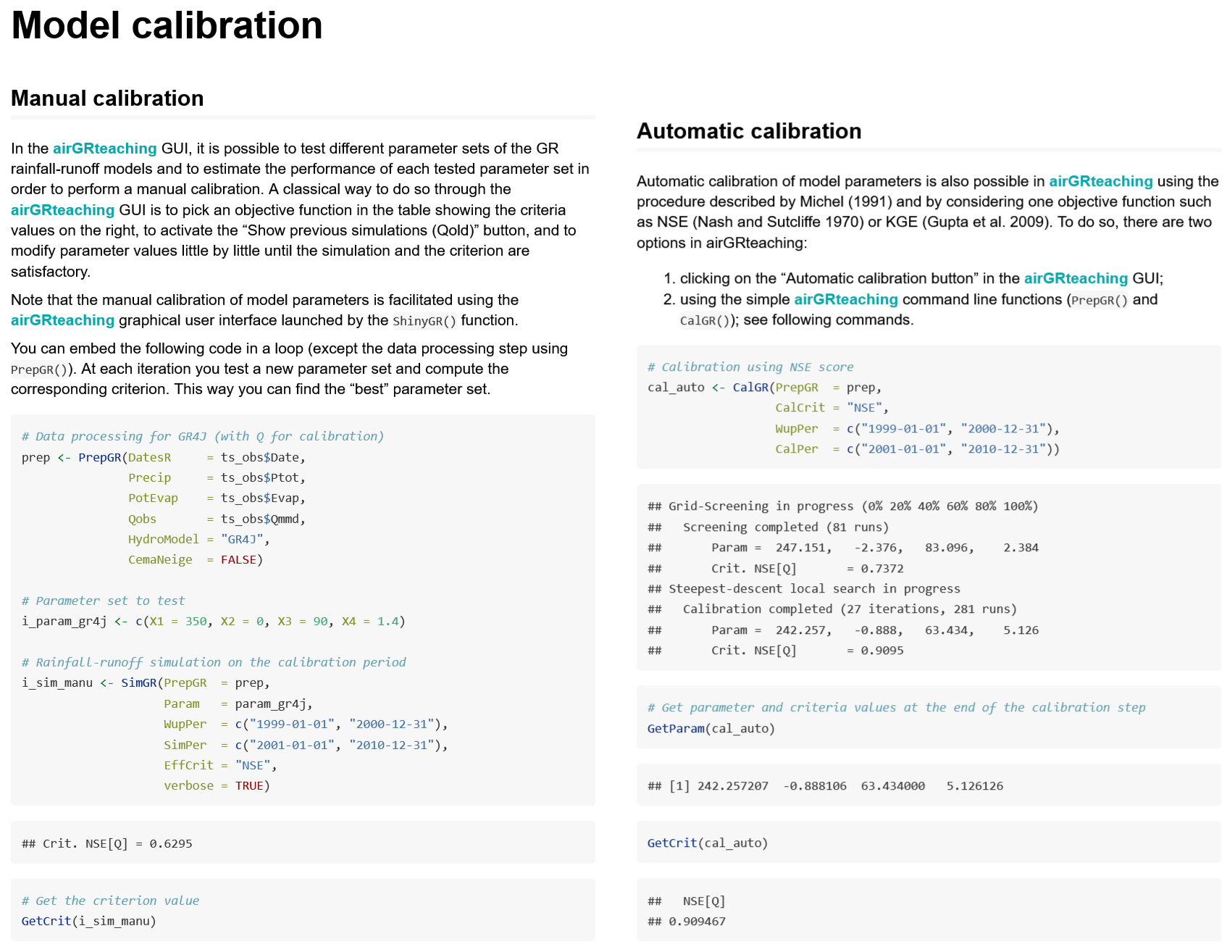
Figure 11 Example of a vignette explaining how to perform both manual (left) and automatic (right) calibration of model parameters using the airGRteaching package.

1. Streamflow reconstruction. The Estéron at Broc catchment presents flow observation from 1999 to 2018 but also several missing data in 2004. This project aims to use the hydro-climatic series available and the GR2M model to reconstruct the missing flow data through rainfall-runoff simulation. The concepts addressed and the skills developed with this project are (i) parameter calibration (both manually and automatically) using an objective function and (ii) calibration–evaluation methodology.

2. Low-flow forecasting. This project aims to use the hydro-climatic data available for the Meuse at Saint-Mihiel catchment and the GR6J rainfall-runoff model to forecast the flows for the autumn of 2018, using (i) the last observed streamflow value, (ii) historical rainfall observations, and (iii) historical flow observations (see Fig. 12). The concepts addressed and the skills developed with this project are (i) the definition of climatology, (ii) flow forecasting, and (iii) flow assimilation.

3. Impact of climate change on streamflow regime. Using catchment-scale delta-change-derived future climate projections, this project aims at quantifying the impact of climate change on the flow regime of the Durance at Embrun catchment (see Fig. 13). The concepts addressed and the skills developed with this project are the (i) delta-change method, (ii) flow regime, (iii) bias correction, and (iv) impact of snow on the flow regime.

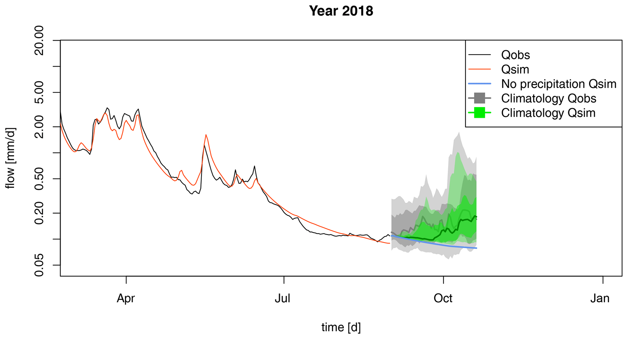
Figure 12 Final output of the airGRteaching “Low-flow forecasting” vignette: observed flow (in black), simulated flow (in red), and different forecast scenarios (in blue: simulated streamflow based on the pessimistic zero precipitation scenario; in gray: streamflow quantiles (10 %, 25 %, 50 %, 75 %, and 90 %) based on historical past flow observations; in green: simulated streamflow quantiles (10 %, 25 %, 50 %, 75 %, and 90 %) based on the precipitation climatology).

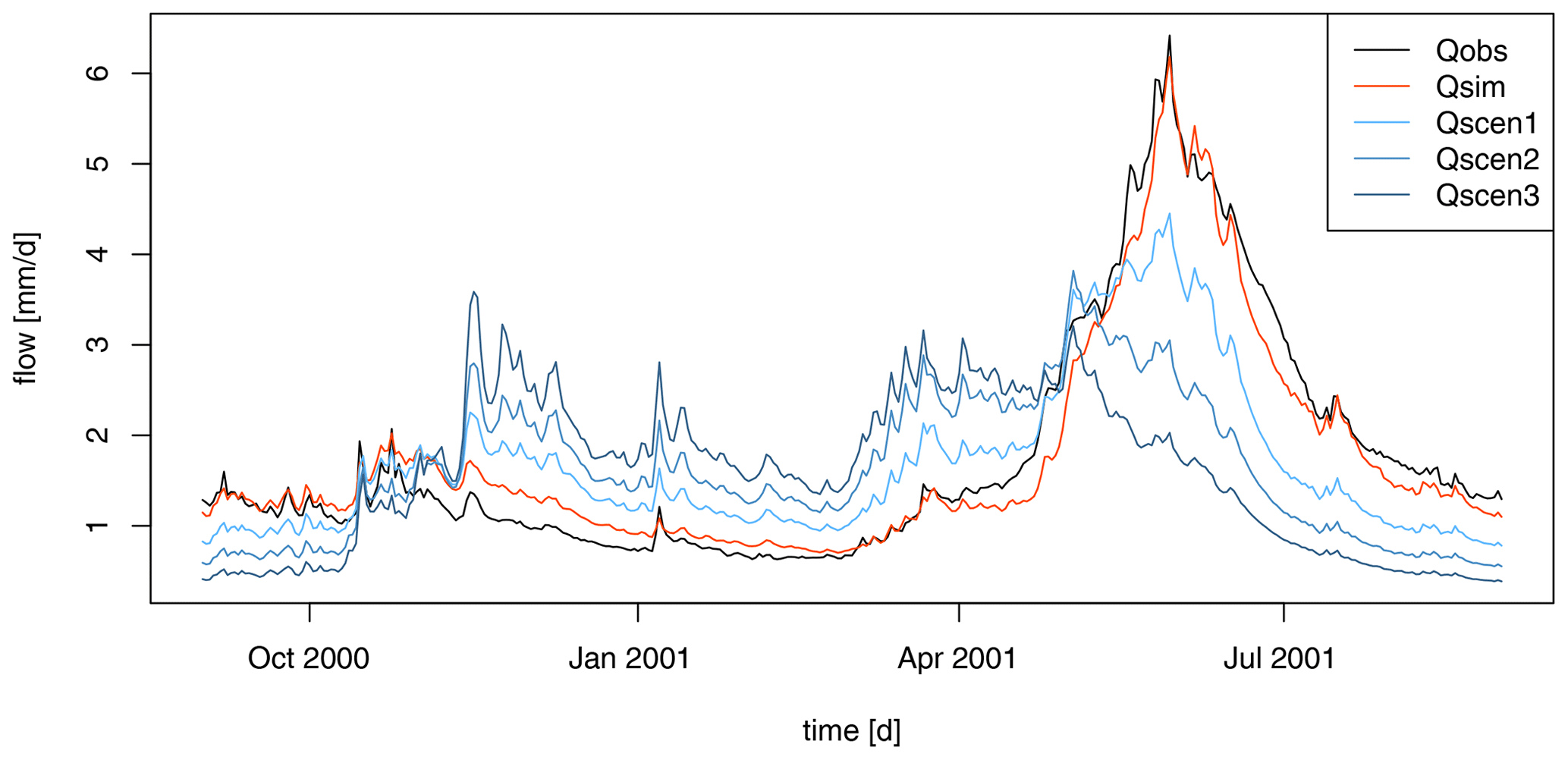
Figure 13 Final output of the airGRteaching “Impact of climate change on streamflow regime” vignette: flow regimes observed (in black), calibrated over the historical period (in red), and simulated using different climate change scenarios (in blue gradient).

Users of the airGRteaching package may also produce their own exercises as airGRteaching vignettes, based on the three examples provided.

We believe that the proposed exercises and projects are a must if one wishes to learn hydrological modeling. They represent the core of many catchment-related studies.

5 Limitations and perspectives

5.1 Limitations

Like any tool, airGRteaching has its limitations. The first one is that so far only GR hydrological models have been available in airGRteaching. Adding other models is feasible, but to do so, they should be implemented to be compatible with the airGR framework (which contains the basic components for airGRteaching). While for the command-line use of airGRteaching (i.e., use of the PrepGR(), CalGR(), and SimGR() functions), this should be easy to implement, the GUI implementation would require more efforts (for instance, it would require the adding of a model scheme for each model; the interface could become less handy, with models presenting over 10 parameters to optimize, and calibration would be far less rapid).

In addition, it is not possible for the user to build their own hydrological model by adding, for example, reservoirs (e.g., with different discharge functions) and unit hydrographs, to help understand each compartment of a model. This is possible with the RS MINERVE software (García Hernández et al., 2020).

Other limitations, as mentioned in Sect. 2.3, are that airGRteaching only offers a limited set of modeling options, compared to airGR. This however could also be seen as a strength, as proposing too many options could be cumbersome from a user's perspective, and these limitations are therefore voluntary.

Remote sensing data, other than meteorological or hydrological data, cannot be used in airGRteaching at the moment. In addition, the effect of land cover changes cannot directly be an asset to airGRteaching, as is the case in some physically based models.

Finally, proper uncertainty exercises, apart from the calibration on different periods, have so far not been a part of this tool, which we see as a simple way of starting hydrological modeling. However, it is easy enough to add noise to the input data to assess input uncertainty. Uncertainty arising from model structure can only be studied by changing models (e.g., using GR4J and GR5J models). The uncertainty associated with parameter calibration methods cannot be tested, as only an optimization algorithm is provided (NB: other algorithms can be plugged into airGR). Finally, airGRteaching does not provide turnkey tools for visualizing uncertainty (e.g., error bars or envelopes on streamflow simulation).

5.2 Perspectives

Exercises linking hydrology with other disciplines and scientific communities could be developed by the coupling of the airGRteaching package with other numerical tools and models. First, using actual global (GCM) or regional (RCM) climate model outputs as rainfall-runoff model inputs would illustrate the impact of climate variability or emission scenarios on catchment hydrology, linking climatology and hydrology. In a similar way, streamflows produced by the airGRteaching package could be used as inputs to hydraulic models to produce flood maps in teaching projects involving both hydrological and hydraulic skills. Finally, coupling airGRteaching with models of water uses (e.g., water withdrawal models for drinking water or irrigation) would have interesting teaching applications. Another valuable perspective is to use remote sensing data to perform data assimilation for hydrological forecasting by recovering real-time meteorological (e.g., precipitation measured by rain gauges), hydrological (e.g., streamflow observed from gauging stations), or even satellite data (e.g., MODIS snow cover observations) and using these data as inputs of a rainfall-runoff model in the airGRteaching package, e.g., with the airGRdatassim package (Piazzi et al., 2021; Piazzi and Delaigue, 2021). Such applications would illustrate the added value of assimilating hydro-meteorological data for better modeling in hydrology. Other exercises could be centered around uncertainties, through coupling the airGRteaching package with sensitivity analysis methods.

Finally, the airGRteaching package could be used for the development of serious games devoted to hydro-meteorological applications, aiming, for example, to discuss the issues of making better decisions when considering probabilistic forecasts (Ramos et al., 2013).

The authors' experience with different audiences has shown that airGRteaching is useful in helping students understand a variety of basic concepts: from the choice of an objective function to the sensitivity of model simulations to individual parameters, the difference between model states and model parameters, the difference between automatic and manual calibration, and the informative and complementary value of a variety of plots. Projects that are more elaborate have been developed and are listed in Sect. 4. For students, depending on the time allotted and their experience, we use the graphical interface with or without the use of computer code. For researchers, it is more a matter of introducing them specifically to GR models, and the interface is used as an introduction of the GR model structure. For engineers working in consulting firms, it is often somewhere in between, depending on their experience and their background. The GUI is frequently used to avoid being bogged down in problems of form and to concentrate exclusively on the underlying concepts of hydrological modeling. The simplified code version allows a smooth transition to the more complex airGR code. For the general public, the aim is usually to introduce them using the airGRteaching GUI to one of the fields of hydrology, to help them understand what a model is, and to raise their awareness of applications such as flood and low-flow forecasting and global change.

The introduction to computer programming is ideal to teach these notions to students. If students are to take this tool into their own hands, they must gradually acquire the concepts without difficulty. It is therefore essential that this is done in a playful way so that they are not discarded. The use of a graphical interface allowing modeling notions to be acquired, while putting aside the programming aspects, allows the different problems to be separated: modeling on the one hand and programming on the other hand. As soon as they wish to go further in the understanding of their subject, students very quickly perceive the limitations that a graphical interface can represent (options too limited, etc.). In addition, use can quickly become daunting if tasks need to be repeated (for example, clicking a large number of times and in a well-defined order to reproduce the results on several datasets). Sometimes there is not enough time to learn programming, justifying the need to use simple tools.

As such, the airGRteaching tool is not intended to be used to realize extended hydrological research studies, and therefore it does not aim to be used to contribute to the actual solving of any of the 23 UPHs (unsolved problems in hydrology; Blöschl et al., 2019). However, as it is a tool to teach hydrology, to understand hydrological processes, and to master hydrological modeling, we believe that airGRteaching could be used as a preliminary step in the solving of some UPHs. Namely, UPH19 (“How can hydrological models be adapted to be able to extrapolate to changing conditions, including changing vegetation dynamics?”) and UPH20 (“How can we disentangle and reduce model structural/parameter/input uncertainty in hydrological prediction?”), due to the many model parameter manipulations and calibration–evaluation exercises that airGRteaching proposes, are good candidates. This tool can contribute to UPH21 (“How can the (un)certainty in hydrological predictions be communicated to decision makers and the general public?”) as it has already been used by several decision makers in hydrological training. airGRteaching can be seen as a gateway to mastering airGR and other airGR-dependent packages, thus indirectly helping to solve other UPHs. This is notably the case for questions UPH22 (“What are the synergies and tradeoffs between societal goals related to water management (e.g., water-environment-energy-food-health)?”) and UPH23 (“What is the role of water in migration, urbanization, and the dynamics of human civilizations, and what are the implications for contemporary water management?”), linked to water usage, thanks to the airGRiwrm package (Dorchies et al., 2022), which allows water resources management to be integrated. This package could help to solve problems of spatial heterogeneity and change of scale, namely UPH5 (“What causes spatial heterogeneity and homogeneity in runoff, evaporation, subsurface water and material fluxes (carbon and other nutrients, sediments), and in their sensitivity to their controls (e.g., snowfall regime, aridity, reaction coefficients)?”) and UPH6 (“What are the hydrologic laws at the catchment scale and how do they change with scale?”) because it simplifies the use of airGR in a semi-distributed mode. The airGRdatassim package, which enables data assimilation, could be linked to questions of prediction uncertainty, namely UPH20.

6 Conclusions

Teaching hydrological modeling requires hands-on experience with rainfall-runoff models. Dedicated tools need to be adapted to the skills of the students and users and preferably developed in an open-source programming language to ensure the reproducibility of the results. In this context, the airGRteaching R package has been developed as an add-on to the airGR package, which gathers several lumped rainfall-runoff models widely used by hydrological researchers and practitioners. airGRteaching contains a graphical user interface and allows teachers and students to import their own data and create their own exercises. A specific dataset of 19 different catchments in France is included in the add-on airGRdatasets package. This dataset is composed of hydro-climatic time series (solid and liquid precipitation, potential evapotranspiration, air temperature, and streamflow time series). Finally, three hydrological teaching projects are proposed aimed at (i) using a monthly rainfall-runoff model to reconstruct flow series, (ii) using a daily model to forecast low flows, and (iii) studying the impact of climate change on streamflow of a mountainous catchment. Thanks to its open nature, other projects may be added to the package by airGRteaching users, based on the dataset provided or other datasets.

Appendix A: Static plots produced by the package

In this appendix, we have used the time series of the X045401001 catchment (the Ubaye at Lauzet-Ubaye [Roche-Rousse] – DREAL PACA). The GR5J model, coupled to CemaNeige, was calibrated on the raw flows of the period from 1 January 2001 to 31 December 2004. The objective function used is the KGE.

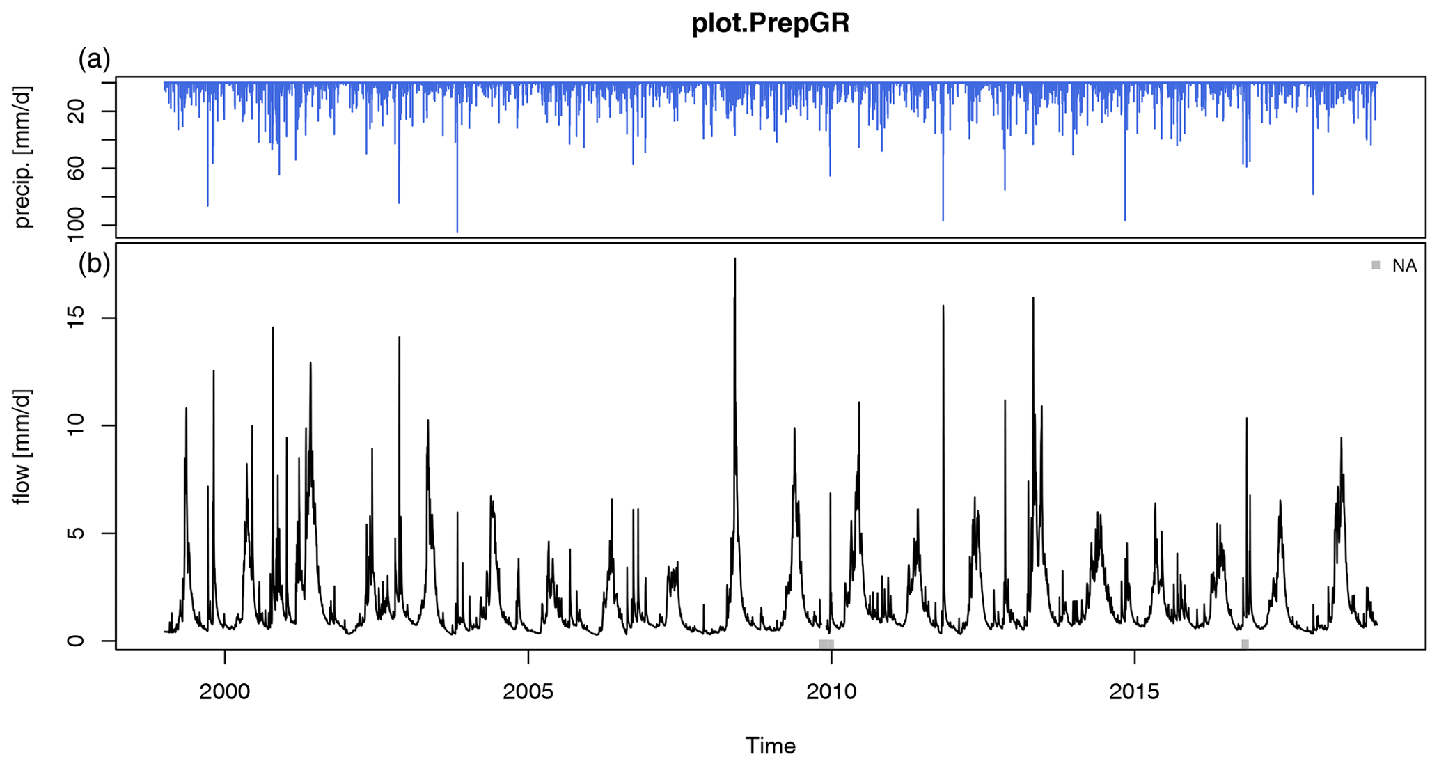
Figure A1 Plot generated using the outputs of the PrepGR() function: (a) precipitation time series and (b) observed hydrograph.

Figure A2 Plot generated using the outputs of the CalGR() or the SimGR() functions, with the argument which  = “synth” (synthesis; default value). From top to bottom and from left to right: (a) precipitation time series (liquid, and solid if CemaNeige is used), (b)  temperature time series for each layer (if CemaNeige is used), (c) snowpack time series for each layer (if CemaNeige is used), (d) observed and simulated hydrographs, (e) monthly average precipitation (liquid, and solid if CemaNeige is used) and 30 d rolling mean of interannual mean daily streamflow, (f) observed and simulated flow duration curves, and (g) scatter plot between observed and simulated discharges. The hydrographs can also be plotted with a log scale.

Figure A3 Plot generated using the outputs of the CalGR() or the SimGR() functions, with the argument which = “perf” (performance). From top to bottom and from left to right: (a) flow error (or residuals), (b) monthly average precipitation (liquid, and solid if CemaNeige is used) and 30 d rolling mean of interannual mean daily streamflow, (c) observed and simulated flow duration curves, and (d) scatter plot between observed and simulated streamflows. The flow error chart can also be plotted with a log scale.

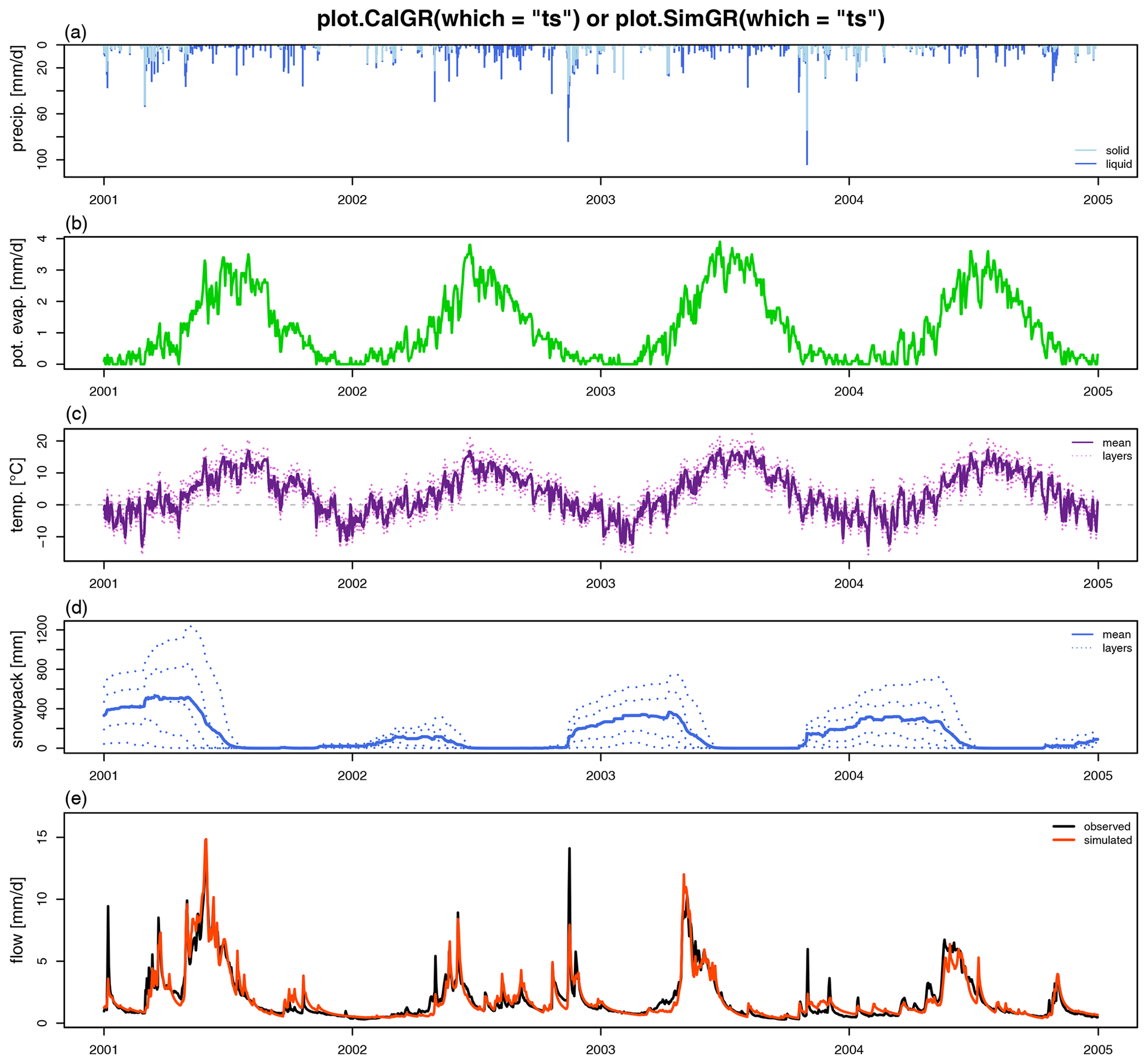
Figure A4 Plot generated using the outputs of the CalGR() or the SimGR() functions, with the argument which = “ts” (time series). From top to bottom: (a) precipitation time series (liquid, and solid if CemaNeige is used), (b) potential evapotranspiration time series, (c) air temperature time series for each layer (if CemaNeige is used), (d) snowpack time series for each layer (if CemaNeige is used), and (e) observed and simulated hydrographs. The hydrographs can also be plotted with a log scale.

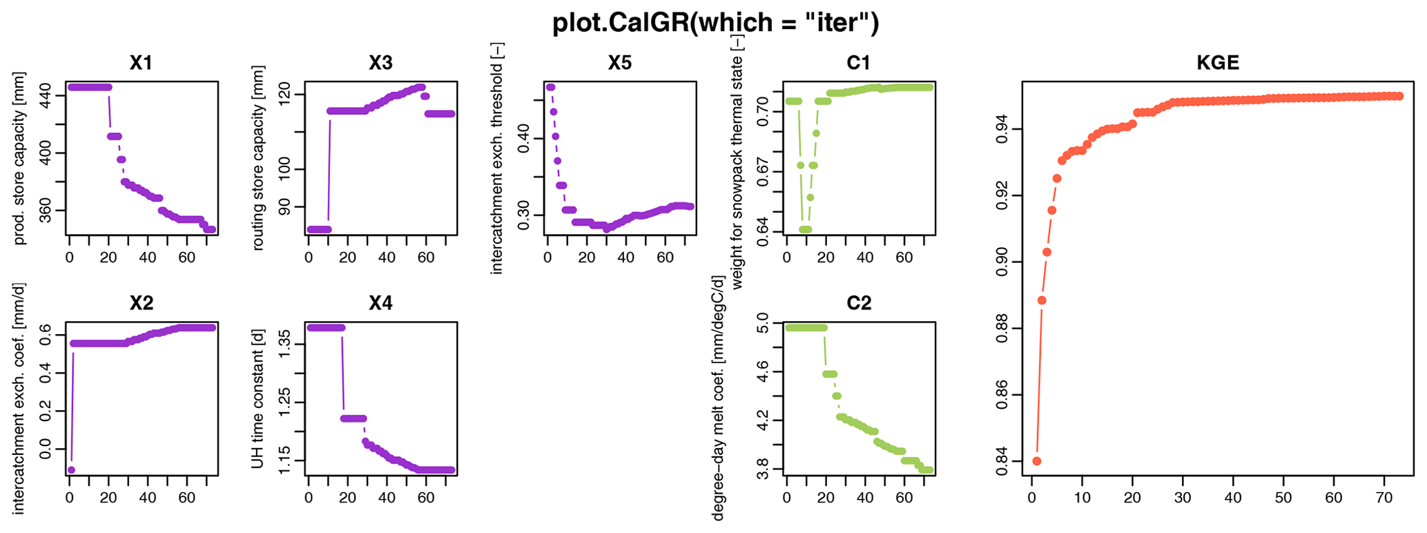
Figure A5 Plot generated using the outputs of the CalGR() function, with the argument which = “iter” (iterations). From left to right: evolution of parameters of the GR5J model (in purple) and CemaNeige model (in green) and of the efficiency criterion (in orange) during the iterations of the steepest-descent calibration step.

Appendix B: Dynamic plots returned by the package

In this appendix, we have used the time series of the X045401001 catchment (the Ubaye at Lauzet-Ubaye [Roche-Rousse] – DREAL PACA). The GR5J model, coupled to CemaNeige, was calibrated on the raw flows of the period from 1 January 2001 to 31 December 2004. The objective function used is the KGE.

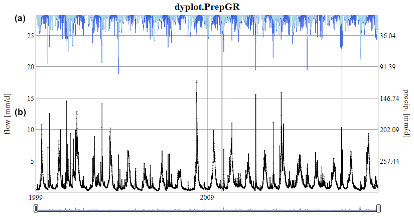
Figure B1 Dynamic plot generated using the outputs of the PrepGR() function: (a) precipitation time series (liquid, and solid if CemaNeige is used) and (b) observed hydrograph.

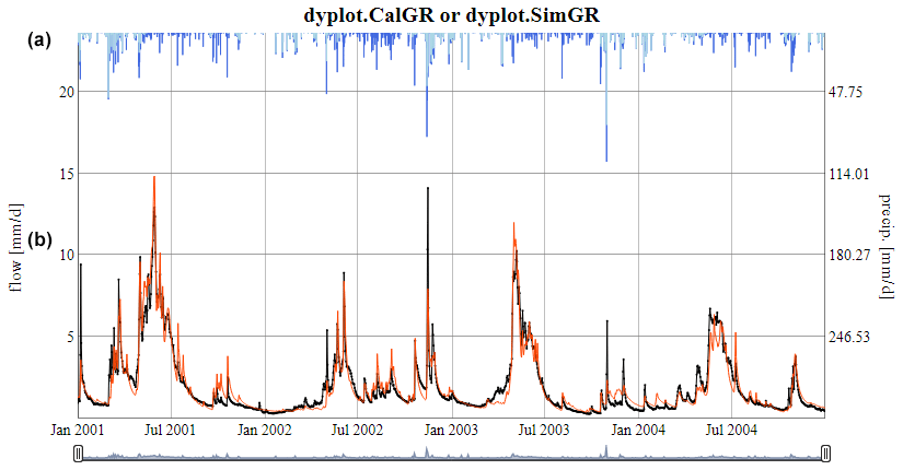
Figure B2 Dynamic plot generated using the outputs of the CalGR() or the SimGR() functions: (a) precipitation time series (liquid, and solid if CemaNeige is used) and (b) observed and simulated hydrographs.

Appendix C: Static plots downloaded from the airGRteaching GUI

In this appendix, we have used the time series of the X045401001 catchment (the Ubaye at Lauzet-Ubaye [Roche-Rousse] – DREAL PACA). The GR5J model, coupled to CemaNeige, was calibrated on the raw flows of the period from 1 January 2001 to 31 December 2004. The objective function used is the KGE.

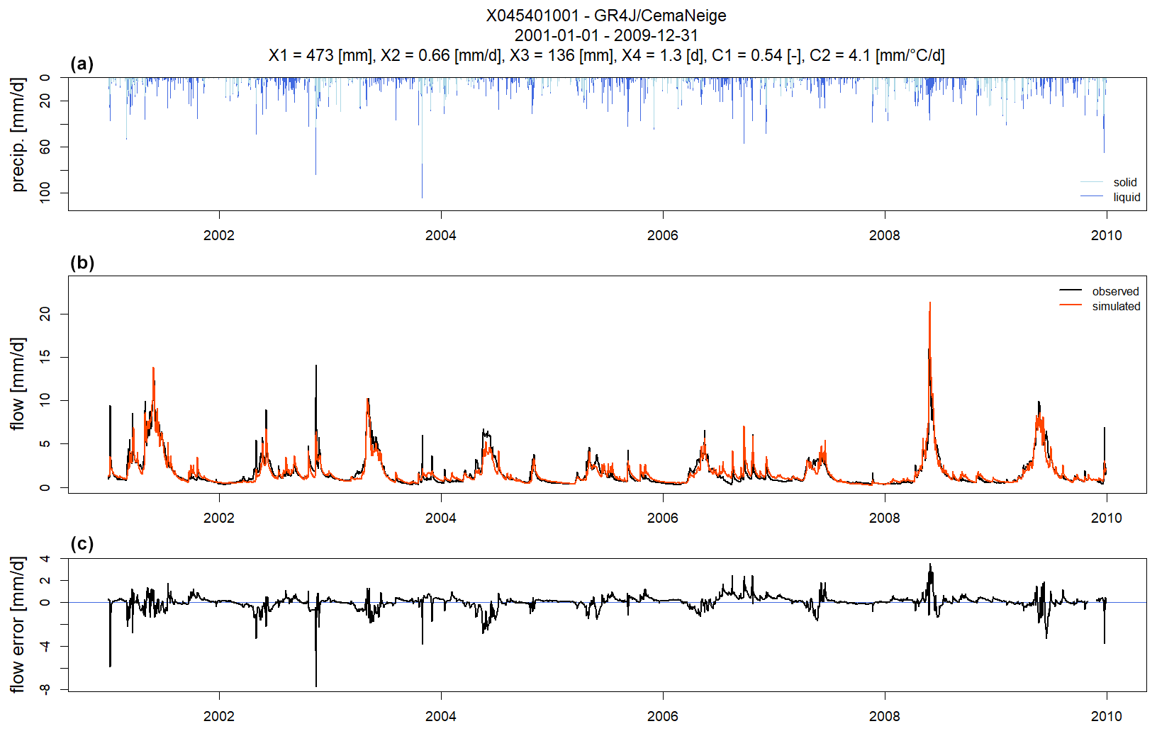
Figure C1 Static plot downloaded from the “Flow time series” tab of the GUI. From top to bottom: (a) monthly average precipitation (liquid, and solid if CemaNeige is used), (b) observed and simulated hydrographs, and (c) flow error time series.

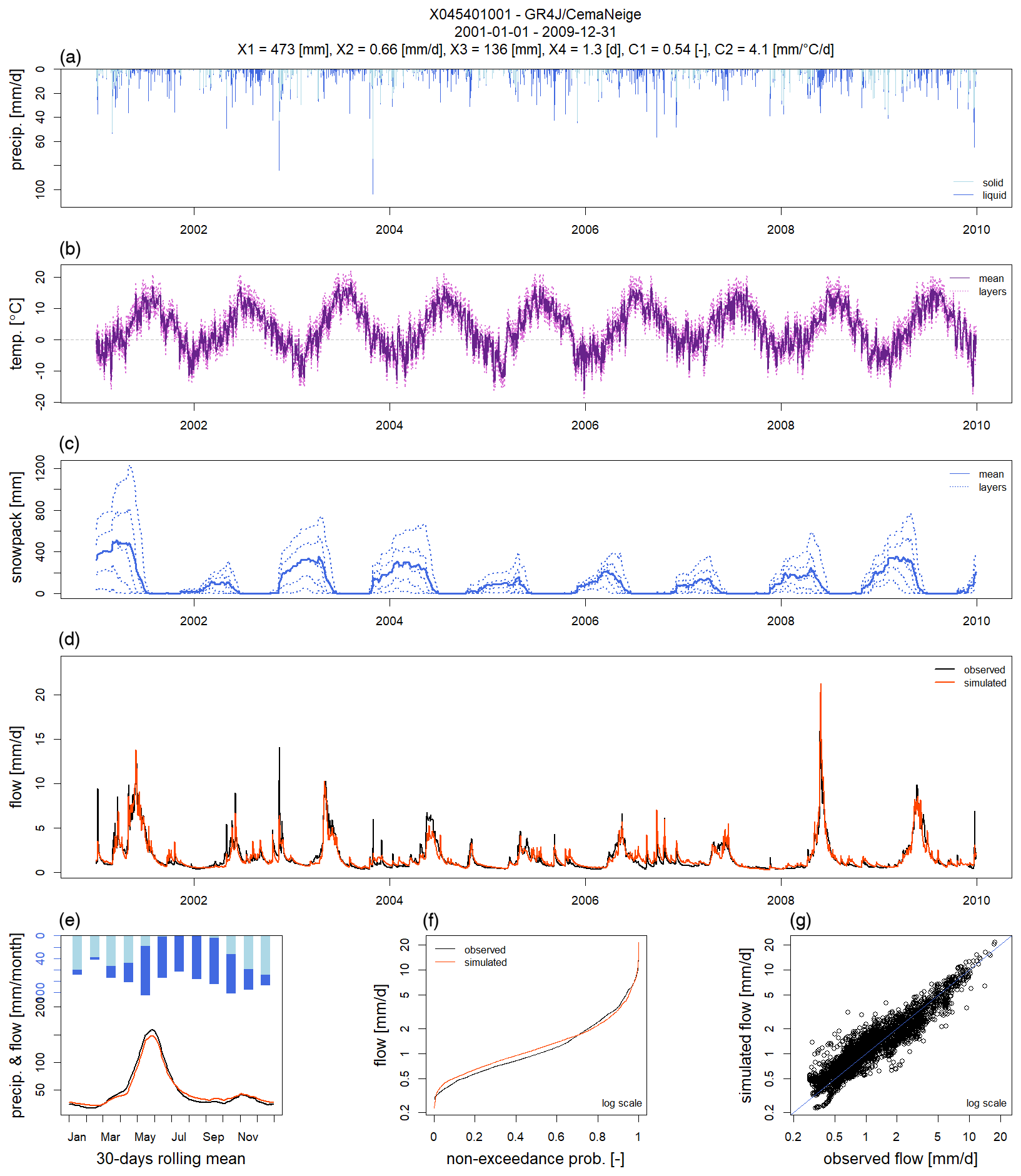
Figure C2 Static plot downloaded from the “Model performance” tab of the GUI. From top to bottom and from left to right: (a) precipitation time series (liquid, and solid if CemaNeige is used), (b) temperature time series for each layer (if CemaNeige is used), (c) snowpack time series for each layer (if CemaNeige is used), (d) observed and simulated hydrographs, (e) monthly average precipitation (liquid, and solid if CemaNeige is used) and 30 d rolling mean of interannual mean daily streamflow, (f) observed and simulated flow duration curves, and (g) scatter plot between observed and simulated discharges.

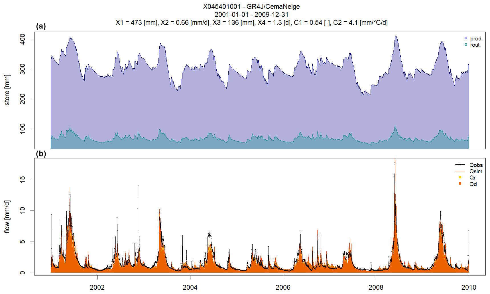
Figure C3 Static plot downloaded from the “State variables” tab of the GUI: (a) time series of store levels and (b) runoff components.

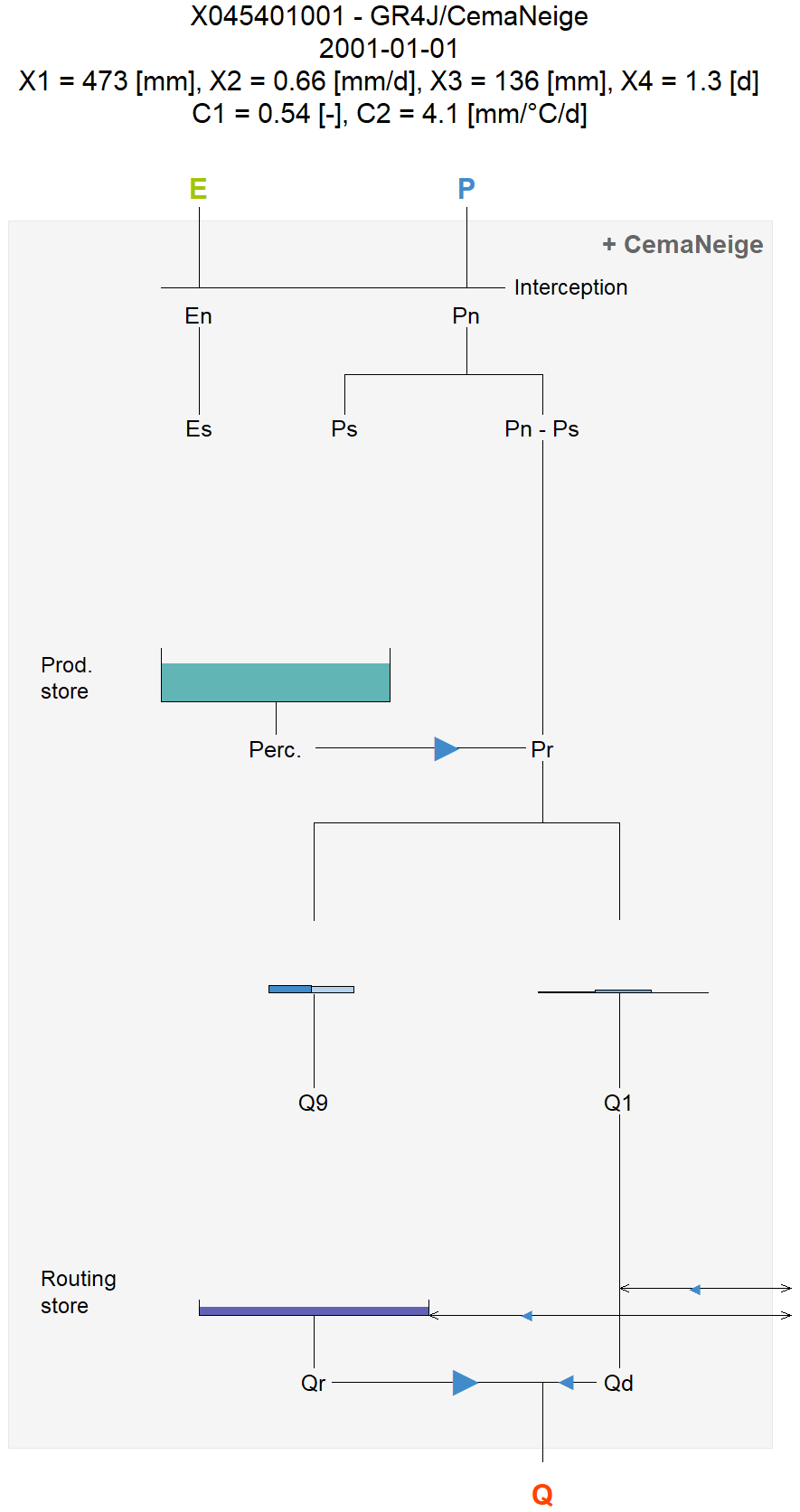
Figure C4 Static plot downloaded from the “Model diagram” tab of the GUI. Model diagram with adaptation of the arrows representing the different fluxes and of the maximal size and the level of the reservoirs according to the actual parameter values and to the values of all internal variables of the model.

Appendix D: “Teaching hydrology with airGRteaching” vignette command lines

Listing D1 Role of the production component in GR4J.

Listing D2 Role of the routing component in GR4J.

Listing D3 Relative importance of the production and routing functions.

Listing D4 On the need to perform a model warm-up.

Listing D5 Manual calibration.

Listing D6 Automatic calibration.

Listing D7 Model evaluation.

Listing D8 Using flow transformation in objective functions.

Listing D9 Using different objective functions.

Listing D10 Split-sample test.

Listing D11 Differential split-sample test.