the Creative Commons Attribution 4.0 License.
the Creative Commons Attribution 4.0 License.
 | 20 May 2021
A note on leveraging synergy in multiple meteorological data sets with deep learning for rainfall–runoff modeling
Daniel Klotz
Sepp Hochreiter
Grey S. Nearing
A deep learning rainfall–runoff model can take multiple meteorological forcing products as input and learn to combine them in spatially and temporally dynamic ways. This is demonstrated with Long Short-Term Memory networks (LSTMs) trained over basins in the continental US, using the Catchment Attributes and Meteorological data set for Large Sample Studies (CAMELS). Using meteorological input from different data products (North American Land Data Assimilation System, NLDAS, Maurer, and Daymet) in a single LSTM significantly improved simulation accuracy relative to using only individual meteorological products. A sensitivity analysis showed that the LSTM combines precipitation products in different ways, depending on location, and also in different ways for the simulation of different parts of the hydrograph.
- Article
(4966 KB) - Full-text XML
- BibTeX
- EndNote


All meteorological forcing data available for hydrological modeling are subject to errors and uncertainty. While temperature estimates between different data products are frequently similar, precipitation estimates are often subject to large disagreements (e.g., Behnke et al., 2016; Timmermans et al., 2019). The most accurate precipitation data generally come from in situ gauges, which provide point-based measurements of rainfall events, which are complex spatial processes (although, in certain cases, especially related to snow, modeled products might be better; e.g., Lundquist et al., 2019). However, large-scale hydrological models require spatial data (usually gridded), which are necessarily model-based products resulting from a combination of spatial interpolation and/or satellite retrieval algorithms, and, sometimes, process-based modeling. Every precipitation data product is based on different sets of assumptions that each potentially introduce different types of error and information loss. It is difficult to predict a priori how methodological choices in precipitation modeling or interpolation algorithms might lead to different types of disagreements in the resulting data products (e.g., Beck et al., 2017; Newman et al., 2019). As an example of the consequences of this difficulty, Behnke et al. (2016) showed that no existing gridded meteorological product is uniformly better than all others over the continental United States (CONUS).
The primary strategy for dealing with forcing uncertainty in hydrological modeling is to use ensembles of forcing products (e.g., Clark et al., 2016). These can be ensembles of opportunity, or they can be drawn from probability distributions, and they can be combined either before (e.g., as precipitation) or after (e.g., as streamflow) being used in one or more hydrological models. In any case, it is generally not straightforward to predict how differences between different forcing products will translate into differences between hydrological model simulations (e.g., Yilmaz et al., 2005; Henn et al., 2018; Parkes et al., 2019), and given that data quality among different products varies over space and time, it is difficult to design ensembling strategies that maximize the information or value of the forcing ensembles.
However, unlike conceptual or process-based hydrological models, machine learning (ML) or deep learning (DL) can use multiple precipitation (and other meteorological) data products simultaneously. This means that it is not necessary to design a priori strategies to combine input forcing data or to combine the outputs of hydrological models forced with different data products. In principle, such models could learn to exploit potential nonlinear synergies in different (imperfect) precipitation data sets or any other type of model input. In particular, deep learning models that are able to learn spatiotemporally heterogeneous behaviors, such as those used by Kratzert et al. (2019a, b), should be able to learn spatiotemporally dynamic effective mixing strategies in the way that they can leverage multiple input products in different locations and under different hydrological conditions. If successful, this could provide a simple and computationally efficient alternative to the ensembling strategies currently used for hydrological modeling.
2.1 Data
This study uses the Catchment Attributes and Meteorological data set for Large Sample Studies (CAMELS; Newman et al., 2014; Addor et al., 2017b). CAMELS contains basin-averaged daily meteorological forcing input derived from three different gridded data products for 671 basins across CONUS. The three forcing products are (i) Daymet (Thornton et al., 1997), (ii) Maurer (Maurer et al., 2002), and the (iii) North American Land Data Assimilation System (NLDAS; Xia et al., 2012). The former product has a 1 km × 1 km spatial resolution, and the latter two have a one-eighth of a degree (approximately 12.5 km × 12.5 km) spatial resolution. Although CAMELS includes 671 basins, to facilitate a direct comparison of results with previous studies, we used only the subset of 531 basins that were originally chosen for model benchmarking by Newman et al. (2017), who removed all basins with an area greater than 2000 km2 and also all basins in which there was a discrepancy of more than 10 % between different methods of calculating the basin area.
Behnke et al. (2016) conducted a detailed analysis of eight different precipitation and surface temperature (daily max/min) data products, including the three used by CAMELS. Those authors compared gridded precipitation and temperature values to station data, using roughly 4000 weather stations across CONUS. Their findings were that “no data set was `best' everywhere and for all variables we analyzed” and “two products stood out in their overall tendency to be closest to (Maurer) and farthest from (NLDAS2) observed measurements.” Furthermore, they did not find a “clear relationship between the resolution of gridded products and their agreement with observations, either for average conditions … or extremes” and noted that the “high-resolution Daymet … data sets had the largest nationwide mean biases in precipitation.”
Figure 1 gives an example of disagreement between precipitation products in CAMELS that we hope to capitalize on by training a model with multiple forcing input. This figure shows the noisy relationship between the three precipitation products in a randomly selected basin (U.S. Geological Survey (USGS) ID 07359610). The idea is that DL should be able to mitigate the type of noise shown in the scatterplot in Fig. 1b.
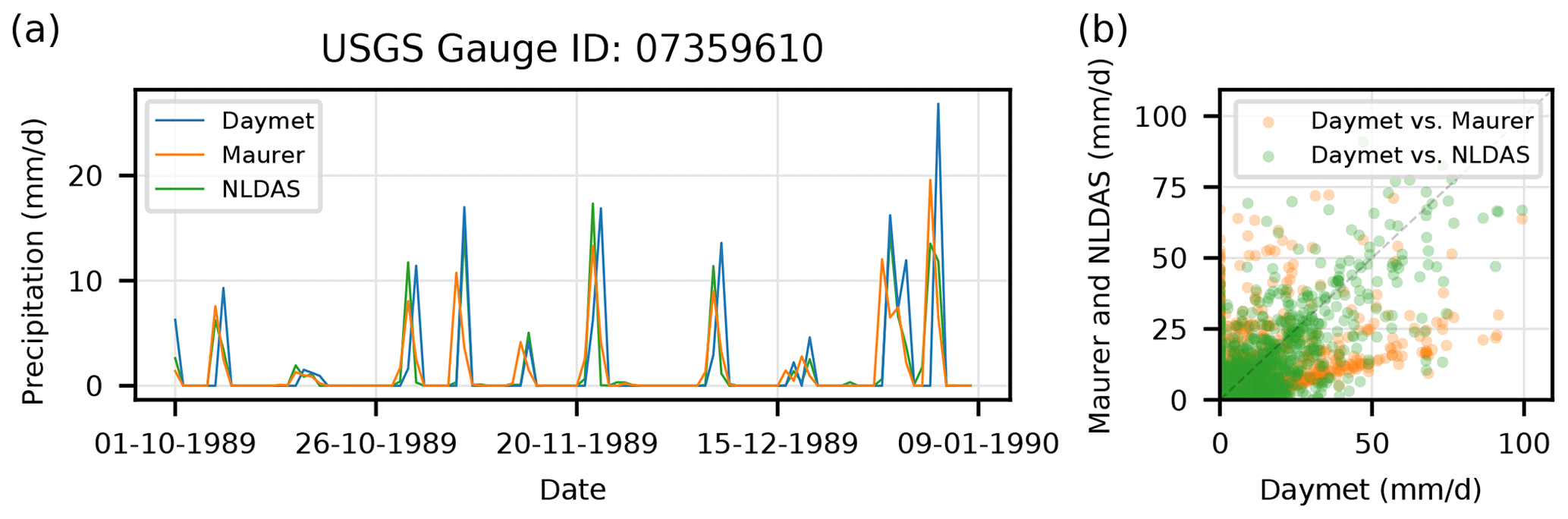
Figure 1Illustration of the relationship between three CAMELS precipitation products at a randomly selected basin (USGS ID 07359610). Panel (a) shows the first 100 d of precipitation data from all three products during the test period, and panel (b) shows scatter between the three products over the full test period. The scatter shown in (b) is the data uncertainty that we would like to mitigate. In this particular basin, there appears to be a 1 d shift between Daymet and Maurer, which is common in the CAMELS data set (this shift is apparent in 325 of the 531 basins; see Fig. 2).
Figure 1a shows a time shift between Daymet and Maurer precipitation in the same basin. This type of shift is common. Behnke et al. (2016), for example, reported that “[because] gridded products differ in how they define a calendar day (e.g., local time relative to Coordinated Universal Time), appropriate lag correlations were applied through cross-correlation analysis to account for the several-hour offset in daily station data.” We performed a lag-correlation analysis on the precipitation products in CAMELS and found a higher correlation between Daymet and Mauer when Mauer was lagged by 1 d in 325 (of 531) basins. Figure 2 shows the percent difference between lagged vs. non-lagged correlations between Daymet and Maurer.
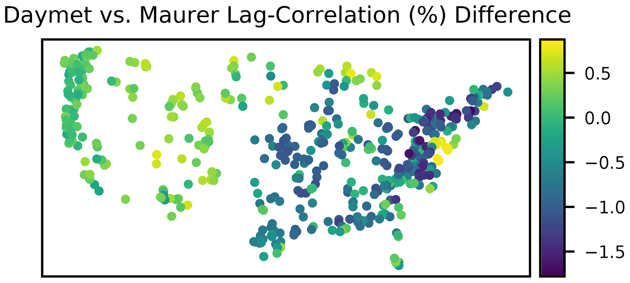
Figure 2Spatial distributions of lagged vs. non-lagged correlations between Daymet and Maurer test period precipitation. Positive values indicate that the 1 d lagged correlation is higher.
Each of the forcing products in CAMELS includes daily precipitation (millimeters per day) and maximum and minimum daily temperature (degrees Celsius), vapor pressure (Pascal), and surface radiation (watts per square meter). The original CAMELS data set hosted by the US National Center for Atmospheric Research (Newman et al., 2014) only contains daily mean temperatures for Maurer and NLDAS. CAMELS-relevant Maurer and NLDAS products, with daily minimum and maximum temperatures, are available from our HydroShare DOI (see the data availability section). We used all five meteorological variables from all three data products as input into the models. In addition to the three daily forcing data sets from CAMELS, we used the same 27 catchment attributes as Kratzert et al. (2019a, b), which consist of topography, climate, vegetation, and soil descriptors (Addor et al., 2017a). Prior to training any models, all input variables were normalized independently by subtracting the CONUS-wide mean and dividing by the CONUS-wide standard deviation.
2.2 Models
Long Short-Term Memory networks (LSTMs) are a type of recurrent neural network (Hochreiter, 1991; Hochreiter and Schmidhuber, 1997b; Gers et al., 2000). LSTMs have a state space that evolve through a set of input–state–output relationships. Gates, which are activated linear functions, control information flows from input and previous states to current state values (called an input gate), from current states to outputs (called an output gate), and also control the timescale of each element of the state vector (called a forget gate). States (called cell states) accumulate and store information over time, much like the states of a dynamical systems model. Technical details of the LSTM architecture have been described in several previous publications in hydrology journals, and we refer the reader to Kratzert et al. (2018) for a detailed explanation geared towards hydrologists.
2.3 Benchmarks
Because all relevant benchmark models from previous studies (see, e.g., Kratzert et al., 2019b) were calibrated using only Maurer forcings, we produced a benchmark using the Sacramento Soil Moisture Accounting (SAC-SMA) model with multiple meteorological forcings. Following Newman et al. (2017), we calibrated SAC-SMA using the dynamically dimensioned search (DDS) algorithm (Tolson and Shoemaker, 2007), implemented in the SPOTPY optimization library (Houska et al., 2019), using data from the training period in each basin. SAC-SMA was calibrated separately, n=10 times with n=10 different random seeds, in each basin for each of the three meteorological data products. This resulted in a total of 30 calibrated SAC-SMA models for each basin.
To check our SAC-SMA calibrations, we compared the performance of our Maurer calibrations against a SAC-SMA model from the benchmark data set calibrated by Newman et al. (2017). We used the (paired) Wilcoxon test to test for significance in any difference between the average, per basin, performance scores from our n=10 different SAC-SMA calibrations with Maurer forcings vs. the SAC-SMA calibrations with Maurer forcings from Newman et al. (2017). The p value of this test was p≈0.9, meaning no significant difference.
Results reported in Sect. 3 used a simple average of these 30 SAC-SMA ensembles in each basin, which is what we found to be the most accurate overall. We also tested (not reported) a Bayesian model averaging strategy, with basin-specific likelihood weights chosen according to relative training performance of the SAC-SMA ensemble members, using Gaussian likelihoods with a wide range of variance parameters. We were not able to achieve an overall higher performance in the test period using an ensembling method more sophisticated than equal-weighted averaging. There are possibilities to potentially improve on this benchmark (e.g., Duan et al., 2007; Madadgar and Moradkhani, 2014); however, as will be shown in Sect. 3, the difference between ensemble averaging and the multi-input LSTMs is large, and we would be surprised if any ensembling strategy could account for this difference.
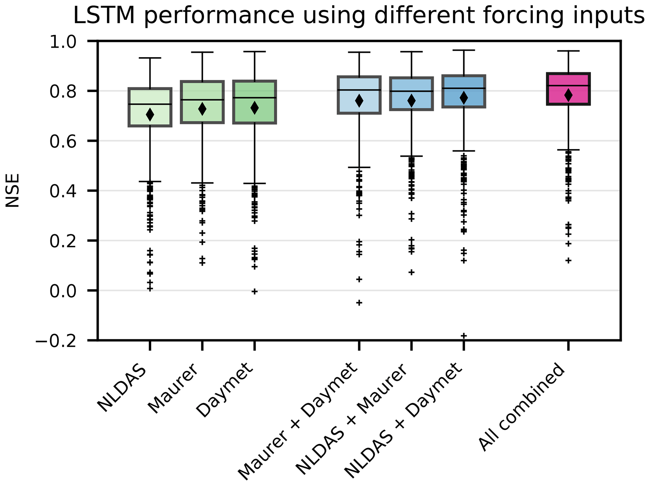
Figure 3Test period comparison between single-forcing and multiple-forcing LSTM ensembles (n=10) over 531 CAMELS basins. All differences were statistically significant (α=0.001), with the exception of Daymet vs. Maurer (p≈0.08) and NLDAS and Maurer vs. Maurer and Daymet (p≈0.4)
Table 1Description of the performance metrics (top part) and signatures (bottom part) considered in this study. For each signature, we derived a metric by computing the Pearson correlation between the signature of the observed flow and the signature of the simulated flow over all basins. Description of the signatures taken from Addor et al. (2018)
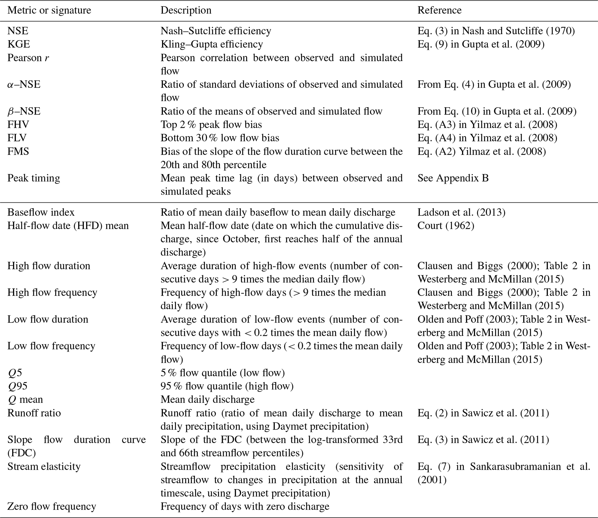
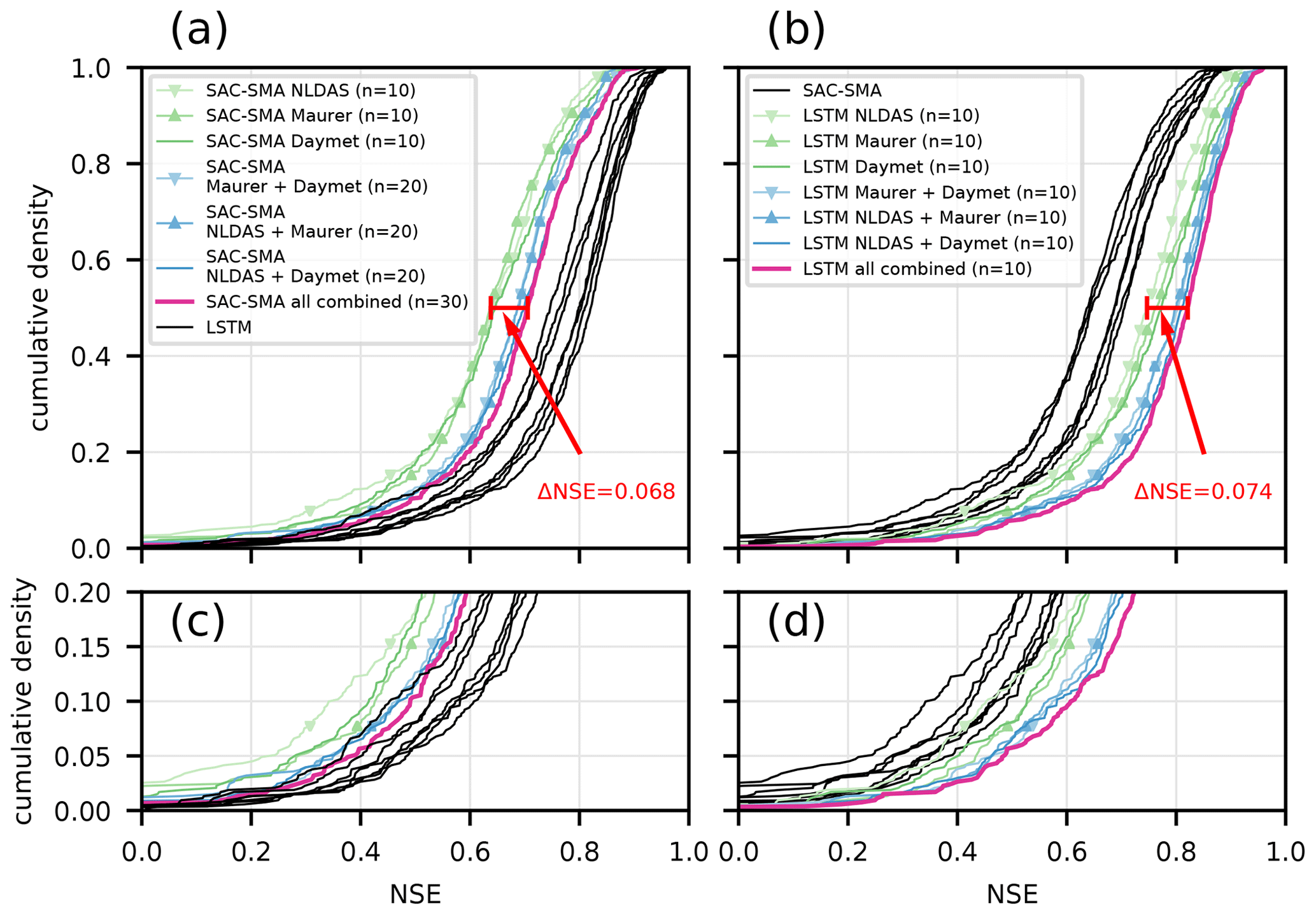
Figure 4Empirical cumulative density function of the NSE performance over the 531 basins of different SAC-SMA ensembles (a, c) and different LSTM ensembles (b, d). Panels (a, b) show the entire range of the cumulative density function, while panels (c, d) show the lower range in more detail. The red indicator lines mark the median NSE difference between the worst single-forcing ensemble and the multi-forcing ensemble of the LSTM and SAC-SMA, respectively.
2.4 Experimental design
We trained n=10 LSTMs using (1) all of the three forcing products together, (2) for each pairwise combination of forcing products (Daymet and Maurer, Daymet and NLDAS, and Maurer and NLDAS), and (3) separately for all three forcing products individually.
For each of these seven input configurations, we trained an ensemble of n=10 different LSTMs with different randomly initialized weights. We report the statistics from averaging the simulated hydrographs from each of these 10-member ensembles (single model results are provided in Appendix A). Ensembles are used to account for the randomness inherent in the training procedure. The importance of using ensembles for this purpose was demonstrated by Kratzert et al. (2019b). Notice that ensembles are used here to mitigate a different type of uncertainty than when using ensembles for combining forcing products. In this case, the model learns how to (dynamically) combine forcing products, and ensembles are used for the same reason as proposed by Newman et al. (2017), i.e., to account for randomness in the calibration and/or training.
The training period was from 1 October 1999 to 30 September 2008 (9 years of training data for each catchment), and the test period was 1 October 1989 to 30 September 1999 (10 years of test data for each catchment). A single LSTM was trained on the combined training period of all 531 basins. Similar to previous studies (Kratzert et al., 2019a, b), we used LSTMs with 256 memory cells and a dropout rate of 0.4 (40 %) in the fully connected layer that derives network predictions (streamflow) from LSTM output. All models were trained with a mini-batch size of 256 for 30 epochs, using the Adam optimizer (Kingma and Ba, 2014) with an initial learning rate of , reduced to 5e−4 after 20 epochs, and further reduced to 1e−4 after 25 epochs. All input were standardized to have zero mean and unit variance over all 531 catchments collectively. During model evaluation, negative predictions in the original value space were clipped to zero, i.e., no negative discharges. The loss function was the basin-averaged Nash–Sutcliffe efficiency (NSE; see Kratzert et al., 2019b).
2.5 Analysis
We examined the experiments described above with two types of analyses. The goal is to provide illustrations of how the LSTM leverages multiple forcing products in spatiotemporally dynamic ways.
-
Analysis 1 – feature ablation. An ablation study removes parts of the network to gain a better understanding of the model. We adopted this procedure by removing the different meteorological forcing products in a step-wise fashion and subsequently comparing results using several performance metrics and hydrologic signatures (see Table 1). To provide context, we also benchmarked the LSTMs against ensembles of SAC-SMA models (see Sect. 2.3).
-
Analysis 2 – sensitivity and contribution. We performed an input attribution analysis of the trained LSTM models to quantify how the trained LSTMs leverage different forcing products in different places and under different hydrologic conditions. We concentrated the sensitivity analysis on the precipitation input because (i) precipitation is consistently found to be the most important variable in rainfall–runoff modeling, which is also true for LSTMs (see Frame et al., 2020), and (ii) according to Behnke et al. (2016), there is little difference in other meteorological variables between these data products.
In addition, we performed an analysis that correlates estimated uncertainty in different precipitation products with LSTM performance to help understand in what sense the LSTM is using different precipitation data to mitigate data uncertainty directly. This analysis is presented in Appendix C.
2.5.1 Analysis 1 – feature ablation
All LSTM ensembles were trained using a squared-error loss function (the average of the basin-specific NSE values); however, we are interested in knowing how the models simulate different aspects of the hydrograph. As such, we report a collection of hydrologically relevant performance metrics outlined in Table 1. These statistics include the standard time-averaged performance metrics (e.g., NSE and KGE) and comparisons between observed and simulated hydrologic signatures. The hydrologic signatures we report are the same ones used by Addor et al. (2018). For each hydrologic signature, we computed the Pearson correlation between the signatures derived from observed discharge vs. those from simulated discharge in each basin. Correlation metrics were calculated on simulated vs. observed signatures in all basins.
2.5.2 Analysis 2 – sensitivity and contribution
All neural networks (like LSTMs) are differentiable, almost everywhere, by design. Therefore, a gradient-based input contribution analysis seems natural. However, as discussed by Sundararajan et al. (2017), the naive solution of using local gradients does not provide reliable measures of sensitivity, since gradients might be flat even if the model response is heavily influenced by a particular input data source (which is not necessarily a bad property; see, e.g., Hochreiter and Schmidhuber, 1997a). This is especially true in neural networks, where activation functions often include step changes over portions of the input space – for example, the sigmoid and hyperbolic tangent activation functions used by LSTMs have close-to-zero gradients at both extremes (see also Shrikumar et al., 2016; Sundararajan et al., 2017).
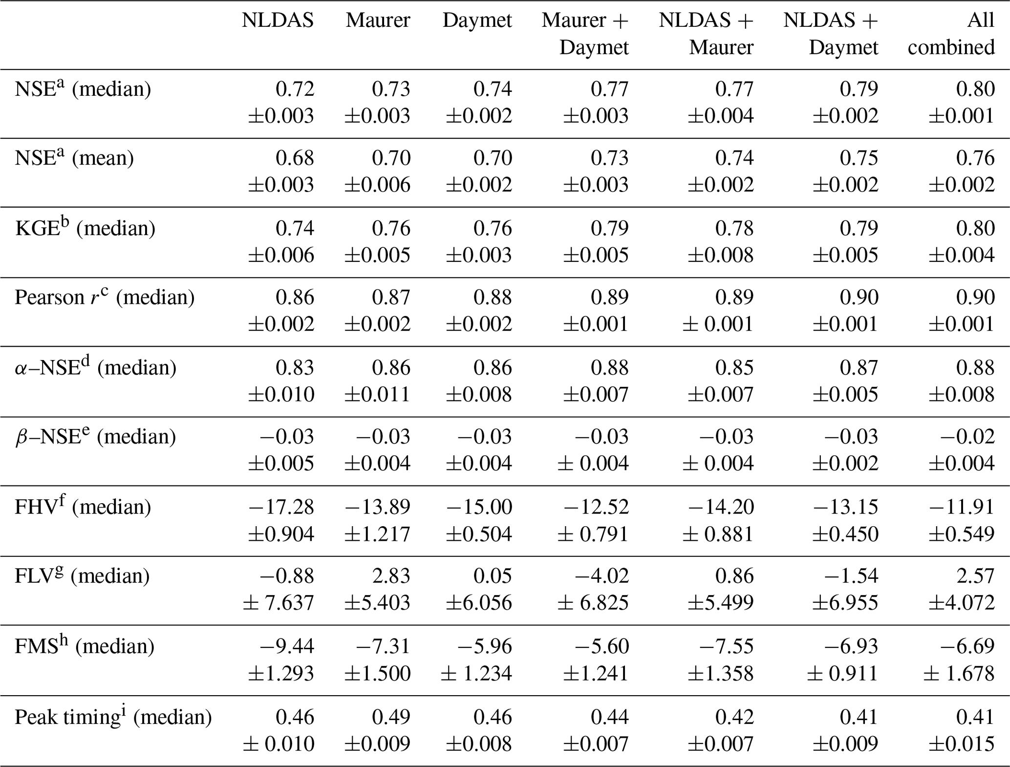
Table 2Values of the benchmarking metrics from Table 1. Bold values indicates the best model (α<0.05). Multiple bold values per row indicate no significant difference.
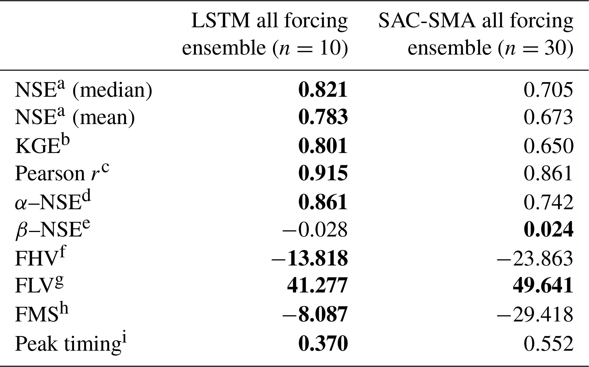
a Nash–Sutcliffe efficiency; ; values closer to 1 are desirable. b Kling–Gupta efficiency; ; values closer to 1 are desirable. c Pearson correlation; ; values closer to 1 are desirable. d α–NSE decomposition; (0,∞); values close to 1 are desirable. e β–NSE decomposition; ; values close to 0 are desirable. f Top 2 % peak flow bias; ; values close to 0 are desirable. g 30 % low flow bias; ; values close to 0 are desirable. h Bias of FDC mid-segment slope; ; values close to 0 are desirable. i Lag of peak timing; ; values close to 0 are desirable.
Table 3Values of the correlation coefficients (over 531 basins) of the simulated vs. observed hydrological signatures from Table 1. Bold values indicate the best model (α<0.05). Multiple bold values per row indicate no significant difference.
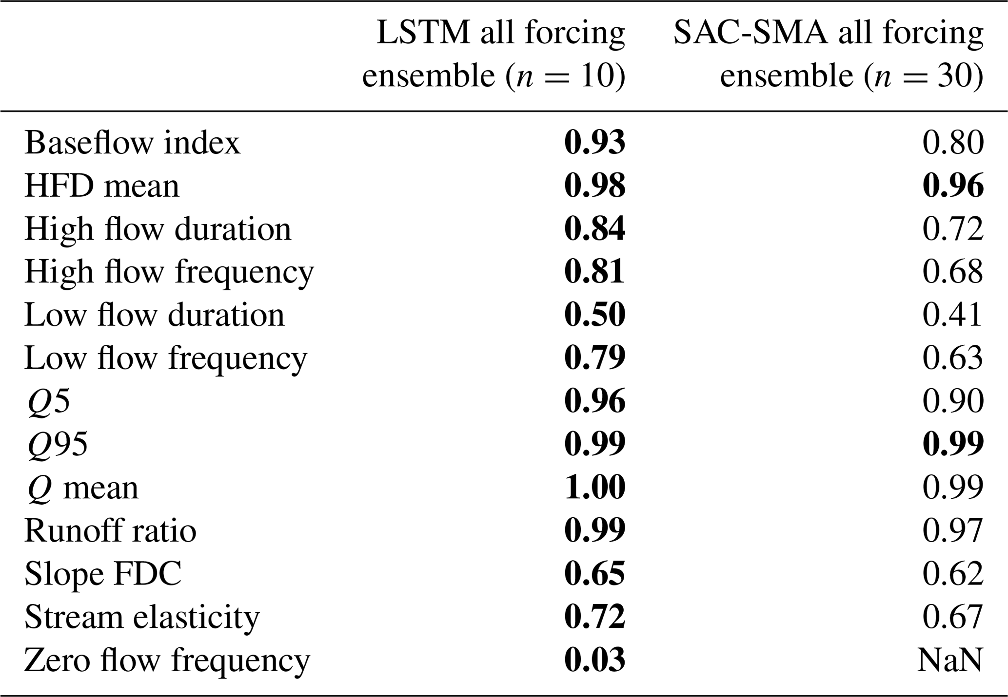
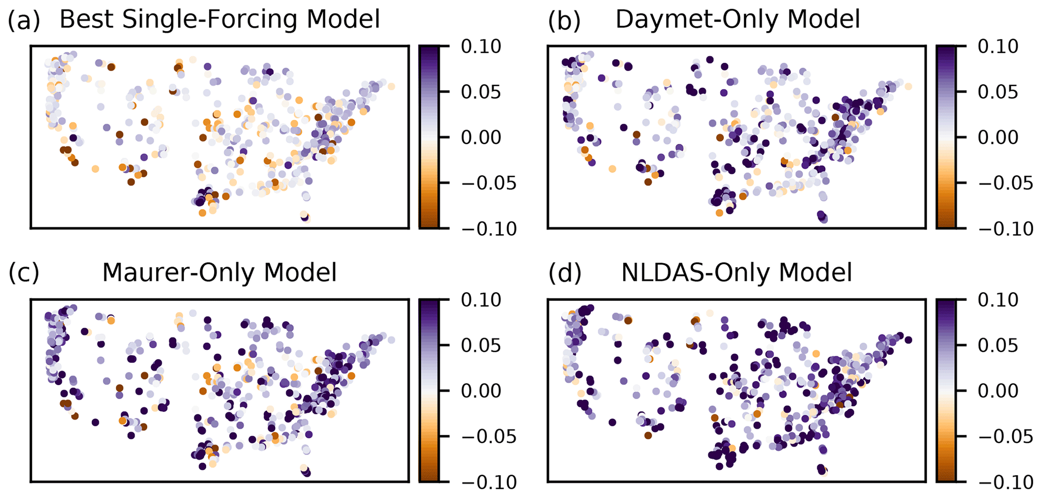
Figure 5Spatial distribution of the NSE differences between the three-forcing LSTM, relative to the best single-forcing model in each basin (a) and relative to each single-forcing model (b–d). Positive (purple) values represent basins where the three-forcing LSTM improved over the single-forcing LSTM. Negative (brown) values reflect basins where the single-forcing LSTM had a higher NSE than the three-forcing LSTM. In total, the three-forcing LSTM was better than the best single-forcing model in 351 of 531 basins (66 %) and was better than each single-forcing model in 443 (83 %; Daymet), 456 (86 %; Maurer), and 472 (89 %; NLDAS) basins, respectively.
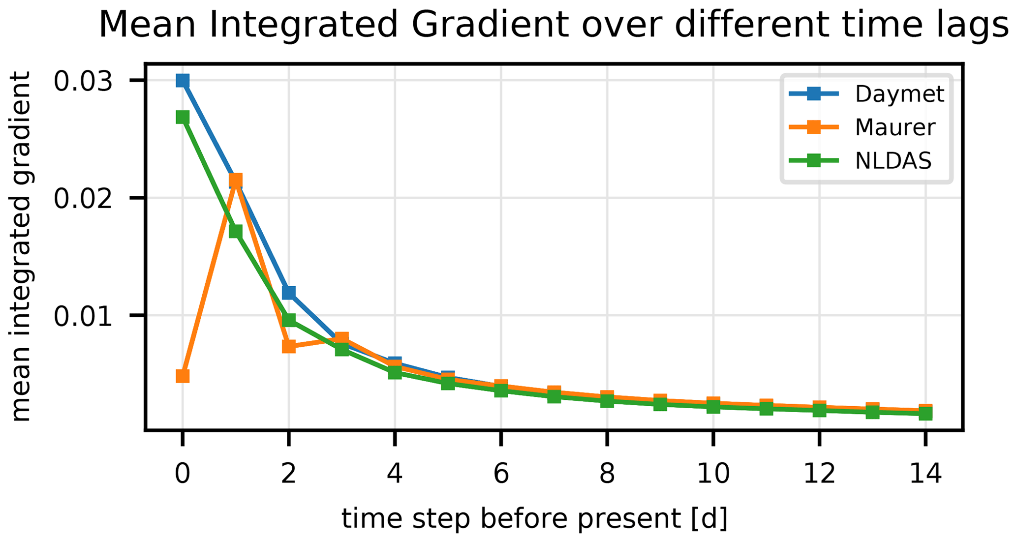
Figure 6Time- and basin-averaged integrated gradients of one of the n=10 multi-forcing LSTMs as a function of lag time (days before current streamflow prediction) of the three precipitation products. Because of the time shift shown in Fig. 2, the model learned to ignore the Maurer input at the current time step.
Sundararajan et al. (2017) proposed a method of input attribution for neural networks which accounts for this lack of local sensitivity. This method is called integrated gradients. Integrated gradients are a path integral of the gradients from some baseline input value, x′, to the actual value of the input, x, as follows:
We used a value of zero precipitation everywhere as the baseline for calculating integrated gradients with respect to the three different precipitation forcings (Daymet, Maurer, and NLDAS). We calculated the integrated gradients of each daily streamflow estimate in each CAMELS basin during the 10-year test period with respect to precipitation input from the past 365 d (the look-back period of the LSTM). That is, on day t=T, we calculated integrated gradient values related to the three precipitation products. The relative integrated gradient values quantify how the LSTM combines precipitation products over time, over space, and also as a function of lag or lead time into the current streamflow prediction. In theory, one has to take the “explaining away” effect into account when analyzing the decision process in models (Pearl, 1988; Wellman and Henrion, 1993). However, we assume that, if evaluated over hundreds of basins and thousands of time steps, this effect is largely averaged out, and therefore, the analysis provides an indication of the actual information used by the model.
3.1 Analysis 1 – feature ablation
The feature ablation analysis compared NSE values over 10-year test periods from the CAMELS basins for the seven distinct input combinations. As shown in Fig. 3, the three-forcing LSTM ensemble had a median NSE value of 0.82 for the 531 basins. The three-forcing model outperformed all two-forcing models. Similarly, all two-forcing models outperformed all single-forcing models (all improvements were statistically significant at α=0.05 when using the Wilcoxon test). The best single-forcing LSTM had a median NSE of 0.77. This indicates that the LSTM was able to leverage unique information in the precipitation signals (this is not an unusual finding in the context of machine learning; see, e.g., Sutton, 2019). We also note that the single-forcing LSTM with Maurer input outperformed the single-forcing NLDAS model, which agrees with the results of Behnke et al. (2016), who showed that Maurer precipitation was generally more accurate than NLDAS precipitation.
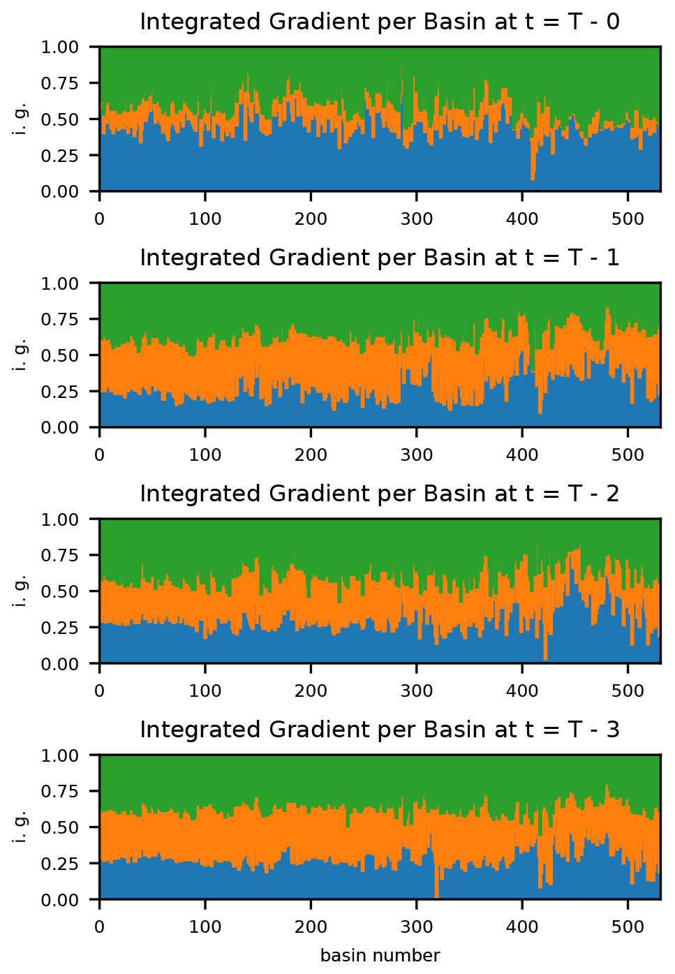
Figure 7Expansion of Fig. 6 by individual basins and truncated at a lag of s=3. The relative importance of Daymet is shown in blue, Maurer in orange, and NLDAS in blue. The multi-forcing LSTM combined the precipitation products in different ways in different basins. Daymet is generally more important in high-number basins located in the Pacific Northwest.
To put these results into context, Fig. 4 compares all LSTMs against benchmark hydrology models, which are all ensembles of SAC-SMA models that were calibrated for each of the three different forcings. All LSTM models were better than all corresponding benchmark models through the entire cumulative distribution function (CDF) curve. The following points can be seen in Fig. 4. First, the SAC-SMA sees a large improvement from using two-forcing products ensembles; this improvement was larger than the corresponding improvement in the LSTMs. However, adding calibrated SAC-SMA models from a third data product did not increase the performance by much (see, e.g., Fig. 4a, where the NLDAS and Daymet ensemble CDF overlaps, most of the time, with the three-forcing ensemble). In contrast, CDFs of the LSTM results show a constant improvement from one- to two-forcing models and from two- to three-forcing models.
Second, the difference between the worst single-forcing ensemble and the three-forcing ensemble is larger for the LSTM (ΔNSE = 0.074) than for the SAC-SMA (ΔNSE = 0.068). This difference could arise from the fact that the LSTM is better able to handle the data shift of the Maurer forcings that occurs in some of the basins (see Sect. 3.2), while this is impossible for the SAC-SMA ensemble.
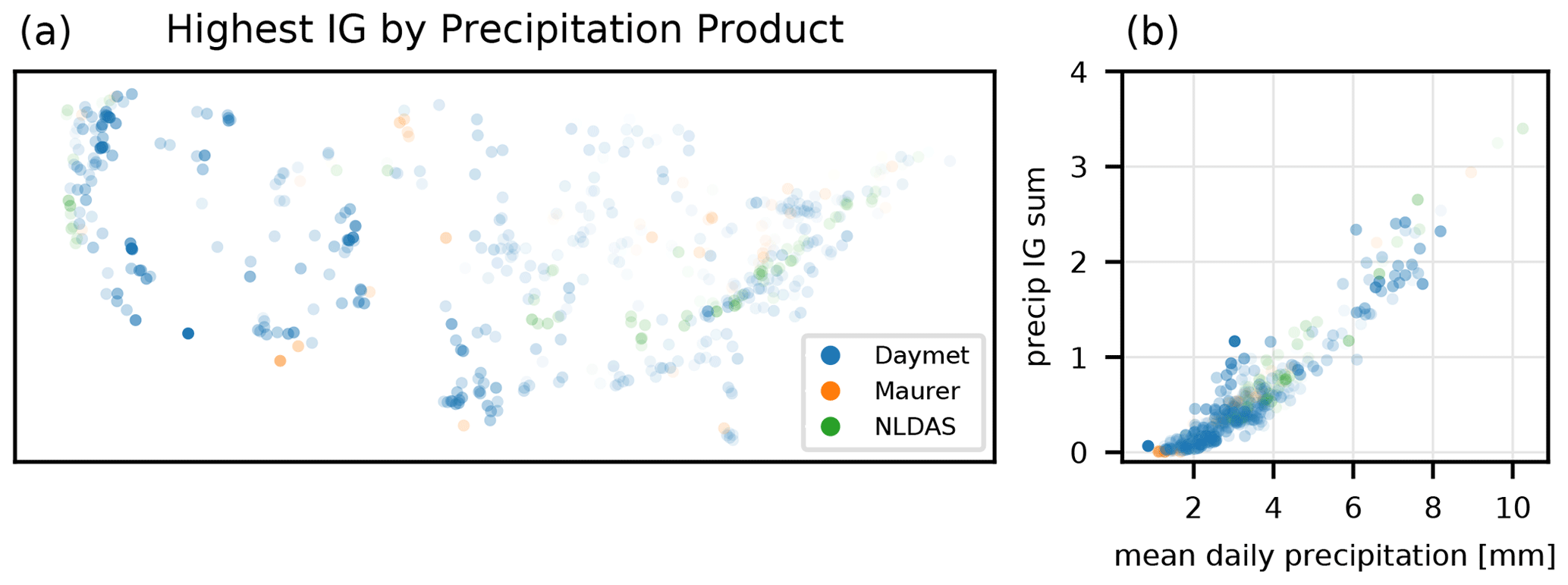
Figure 8The forcing product, with the highest overall contribution (sensitivity) in each basin (a), averaged over the prediction time step and lag. The alpha value (opacity) of each dot on this map is a relative measure of the fraction of the total integrated gradients of all three precipitation products (summed over time, lag, and product) due to the highest-contributing product. Panel (b) shows that the total integrated gradient summed over all three precipitation products is highly correlated with total precipitation in the basin.

Figure 9Spatial distribution of the highest-ranked precipitation products at specific lags (different rows) over the whole hydrograph (left-hand column), and the rising and falling limbs of the hydrograph (center and right-hand columns, respectively), where blue circles denote Daymet, orange circles denote Maurer and green circles denote NLDAS. The takeaway from this figure is that the multi-forcing LSTM learns to combine the different products in different ways for different memory timescales in different basins and under different hydrological conditions. The alpha value (opacity) of each dot is a relative measure of the fraction of the total integrated gradients of all three precipitation products due to the highest-contributing product.
Third, the worst-performing single-forcing LSTM ensemble (i.e., with NLDAS forcings) was significantly better () than the whole n=30 SAC-SMA ensemble, which uses all three forcing products (i.e., the best SAC-SMA result that we found). In fact, even the average single LSTM (not the full n=10 ensemble) trained with NLDAS forcings is as good as the n=30 SAC-SMA ensemble (see Appendix A for non-ensemble LSTM performances), and the average single LSTM (not the ensemble) trained with Maurer or Daymet forcings was significantly better () than the n=30 SAC-SMA ensemble.
Fourth, the ranking of the forcing products is not as clear for the SAC-SMA ensembles as it was the LSTM ensembles (there is more separation in the LSTM single-forcing CDFs than the SAC-SMA single-forcing CDFs). However, qualitatively, the same ranking is visible, i.e., that Daymet models are better than NLDAS or Maurer and that NLDAS and Daymet produce the best two-forcing results.
Tables 2 and 3 give benchmarking results from all metrics and signatures in Table 1. The three-forcing LSTM significantly out-performed the three-forcing SAC-SMA ensemble in all metrics except β–NSE decomposition, where the SAC-SMA ensemble was better, and FLV, where the difference was not significant (see Table 2). The three-forcing LSTM also significantly out-performed the three forcing SAC-SMA ensemble in all signatures (see Table 3) except the HFD mean and the Q95, where the difference was not significant. Note that the LSTM – while generally providing the best model overall – has approximation difficulties towards the extreme lower end of the runoff distribution (low flow duration, low flow frequency, and zero flow frequency).
Figure 5 shows the spatial distribution of the performance differences between the best single-forcing model and the three-forcing model in all basins. The three-forcing LSTM outperformed the single forcing LSTMs almost everywhere. Individual exceptions, where less is more do, however, exist (e.g., southern California). Concretely, if we compare the three-forcing model to the best performing single-forcing LSTM per basin, the three-forcing LSTM had a higher NSE in 66 % of the basins (351 of 531). When compared to each single-forcing LSTM separately, the three-forcing LSTM had a higher NSE in 443 (83 %; Daymet), 456 (86 %; Maurer), and 472 (89 %; NLDAS) basins, respectively.
3.2 Analysis 2 – sensitivity and contribution
Figure 6 shows the time- and basin-averaged integrated gradient of one of the n=10 multi-forcing LSTMs as a function of lead time. To reiterate the information above, the integrated gradient is a measure of input attribution or sensitivity, such that input with higher integrated gradients have a larger influence on model outputs. Integrated gradients shown in Fig. 6 were averaged over all time steps in the test period and also over all basins. This figure shows the sensitivity of streamflow at time t=T to each of the three precipitation input at times , where s is the lag value on the x axis. The main takeaways from this high-level illustration of input sensitivities are (1) that the sensitivity of current streamflow to precipitation decays with lead time (i.e., time before present) and (2) that the multi-forcing model has learned to ignore the Maurer input at the present time step. The reason for the latter is the time shift in the Maurer product (illustrated in Fig. 2).
Figure 6 shows results from only one of n=10 model repetitions; however, we performed an integrated gradient analysis on all n=10 multi-input LSTMs (not shown), and the results were qualitatively similar. It is difficult to show all the results on the same figure because the values are relative; so, integrated gradients between two different models often have different absolute scales, and the results presented for a single model (in Fig. 6) are representative.
The multi-forcing LSTMs learned to combine the different precipitation products in spatiotemporally variable ways. Figure 6 demonstrates the overall behavior of the multi-forcing LSTM. It is, however a highly condensed aggregate of a highly nonlinear system. As such, a lot of specific information is lost in that figure.
Figure 7 shows integrated gradients by basin and up to a lead time of s=3 d prior to the present. The model largely ignores Maurer precipitation at the current time step in most basins (as was apparent in Fig. 6), but the ratio of the contributions of each product (averaged over the whole test period hydrograph) varies between basins. Figure 7 shows the relative contributions of each precipitation product, but it is important to note that the overall importance of precipitation also varies between basin.
Figure 8 shows the spatial distribution of the most sensitive precipitation contribution (averaged over the whole hydrograph in each basin) in Fig. 8a and the overall sensitivity to all three precipitation products combined in Fig. 8b. The latter (total sensitivity to precipitation relative to all other input) is highly correlated with the total (or average) precipitation in the basin.
It is possible to break the spatial relationship down even further. The spatial distribution of the highest-ranked product as a function of the lag time for rising and falling limits is shown in Fig. 9. This figure shows some of the nuance in how the multi-forcing LSTM learned to combine the different precipitation products by distinguishing between different memory timescales in different basins for different hydrological conditions (i.e., rising and falling limbs of the hydrograph).
The purpose of this paper is to show that LSTMs can leverage different precipitation products in spatiotemporally dynamic ways to improve streamflow simulations. These experiments show that there exist systematic and location- and time-specific differences between different precipitation products that can be learned and leveraged by deep learning. As might be expected, the LSTMs tested here tended to improve hydrological simulations more when there were larger disagreements between different precipitation estimates in a given basin (see Appendix C).
It is worth comparing these findings with classical conceptual and process-based hydrological models that treat precipitation estimate as a unique input. Current best practice for using multiple precipitation products is to run an ensemble of hydrological models, such that each forcing data set is treated independently. Deep learning models have the ability to use a larger number and variety of input than classical hydrology models, and in fact, DL models do not need input that represent any given hydrological variable or process and, therefore, have the potential to use less highly processed input data like remote sensing brightness temperatures, etc. Future work might focus on building runoff models that take as input the raw measurements that were used to create standard precipitation data products.
Deep learning provides possibilities not only for improving the quality of regional (Kratzert et al., 2019b) and even ungauged (Kratzert et al., 2019a) simulations but also, potentially, for replacing large portions of ensemble-based strategies for uncertainty quantification (e.g., Clark et al., 2016) with multi-input models. There are many ways to deal with the uncertainty in traditional hydrological modeling workflows, but almost certainly, the most common approach is to use ensembles. Ensembles can be opportunistic – i.e., from a set of pre-existing models or data products – or constructed – i.e., sampled from a probability distribution – but in either case, the idea is to use variability to represent lack of perfect information. Clark et al. (2016) advocated using ensembles as hydrologic storylines, which would avoid the problem of the sparsity of sampling any explicit or implied probability distributions. No matter how ensembles are used, however, with conceptual and process-based hydrology models, each model takes one precipitation estimate (time series) as input. Multi-input DL models have the potential to provide a fundamentally different alternative for modeling under this kind of uncertainty, since DL models can learn how to combine different input in ways that leverage – in nonlinear ways – all data available to the full simulation task. Future work could focus on producing predictive probabilities with multi-input deep learning models.
Table A1Average single LSTM performance over a variety of metrics. The average single-model performances is computed as the mean of the metric of the n=10 model repetitions.
a Nash–Sutcliffe efficiency; ; values closer to 1 are desirable. b Kling–Gupta efficiency; ; values closer to 1 are desirable. c Pearson correlation; ; values closer to 1 are desirable. d α–NSE decomposition; (0,∞); values close to 1 are desirable. e β–NSE decomposition; ; values close to 0 are desirable. f Top 2 % peak flow bias; ; values close to 0 are desirable. g 30 % low flow bias; ; values close to 0 are desirable. h Bias of FDC mid-segment slope; ; values close to 0 are desirable. i Lag of peak timing; ; values close to 0 are desirable.
Table A2Average single LSTM performance across a range of different hydrological signatures. The derived metric for each signature is the Pearson correlation between the signature derived from the observed discharge vs. the signature derived from the simulated discharge. The average single-model performances are then reported as the mean value of the n=10 model repetitions.

To evaluate the model performance on the peak timing, we used the following procedure: first, we determined peaks in the observed runoff time series by locality search; that is, potential peaks are defined as local maxima. To reduce the number of peaks and filter out noise, the next step was an iterative process where, by pairwise comparison, only the maximum peak is kept until all peaks have at least a distance of 100 time steps to each other. The procedure is implemented in SciPy's find_peak function (Virtanen et al., 2020) and is used in the current work.
Second, we iterated over all peaks and searched for the corresponding peak in the simulated discharge time series. The simulated peak is defined as the highest discharge value inside a window of ±3 d around the observed peak, and the peak timing error is the offset between the observed peak and the simulated peak. The resulting metric is the average offset over all peaks.
The goal of this supplementary analysis was to understand the relationship between precipitation uncertainty and improvements to streamflow simulations due to using multiple forcing data sets. Because we do not have access to true precipitation values in each catchment, we used triple collocation to estimate precipitation uncertainty. Triple collocation is a statistical technique for estimating error variances of three or more noisy measurement sources without knowing the true values of the measured quantities (Stoffelen, 1998; Scipal et al., 2010). Its major assumption is that the error models are linear and independent between sources and, in particular, that all (three or more) measurement sources are each a combination of a scaled value of the true variable plus additive random noise, as follows:
where M* are measurement values (i.e., here the modeled precipitation values), subscript i represents the source (Daymet, Maurer, and NLDAS), and subscript t represents the time step in the test period (1 October 1989 to 30 September 1999). T* is the unobserved true value of total precipitation in a given catchment on a given day, and ε* are independent and identically distributed measurement errors from any distribution.
The linearity assumption is not appropriate for precipitation data, which are typically assumed to have multiplicative errors. Following Alemohammad et al. (2015), we assumed a multiplicative error model for all three precipitation sources and converted these to linear error models by working with the log-transformed precipitation data, as follows:
Standard triple collocation is then applied so that estimates of the error variances for each source are as follows:
for all , where Ci,j is the covariance between the time series of source i and source j, and σi is the variance of the distribution that each independent and identically distributed measurement εi,t is drawn from.
Additionally, extended triple collocation (McColl et al., 2014) allows us to derive the correlation coefficients between measurement sources and truth as follows:
This triple collocation analysis was applied separately in each of the 531 CAMELS catchments to obtain basin-specific estimates of the error variances, σi, and truth correlations, ρi, for each of the three precipitation products. Albeit the assumption that the forcing products have independent error structures (i.e., ) is not met in our case, we expect the results to be robust enough for the purpose at hand.
Daymet typically produced lower NSE values in basins where triple collocation reported that the Daymet precipitation error variances were high. This is what we would expect, i.e., low model skill in basins with high precipitation error. However, we did not see similar patterns with the other two precipitation products (see Fig. C1), where the triple collocation error variances and truth correlation are plotted against the NSE scores of the single-source models. In fact, the NLDAS LSTM tended to perform worse in basins with lower precipitation error (as estimated by triple collocation).
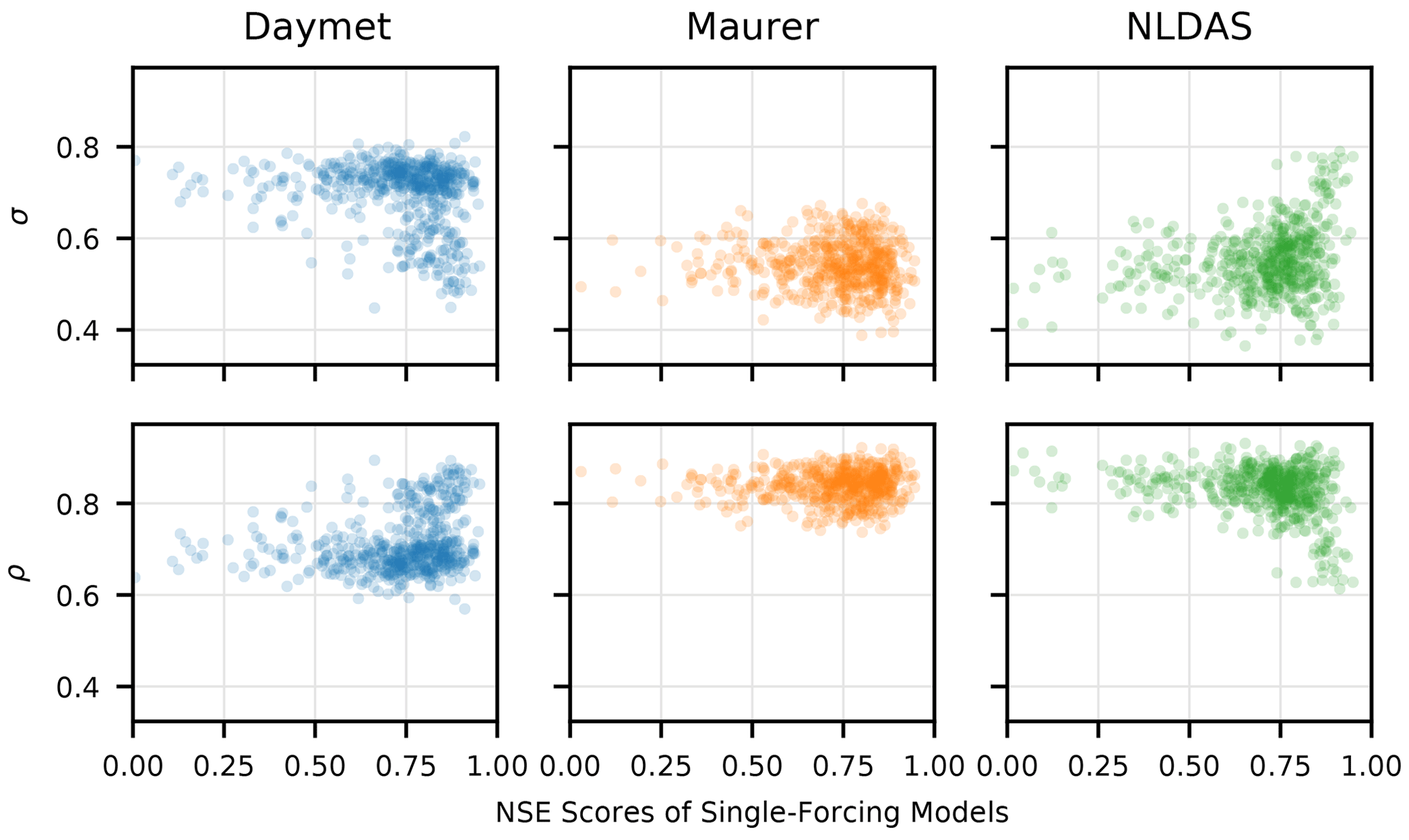
Figure C1Triple collocation error variances (σ – Eq. C4) and truth correlations (ρ – Eq. C5) plotted against NSE scores of the single-forcing LSTM models. ρ describes how much correlation there is between the given data product and the estimated truth, and σ describes the estimated disagreement between a given data product and the other two data products. Daymet typically produces lower NSE values in basins where triple collocation reports that the precipitation error variances are high, whereas NLDAS produces lower NSE values in basins where triple collocation reports that the error variances are low. There is no apparent pattern in the Maurer data.
A reason for this is shown in Fig. C2, which is an adapted version of Fig. C1 that highlights a few high-skill, high triple-collocation-variance NLDAS basins in blue. These basins correspond to a cluster of basins in the Rocky Mountains (Fig. C3) where NLDAS has a low correlation with the other two products but still yields high-skill LSTM simulations. What is happening here is that triple collocation measures (dis)agreement between measurement sources rather than error variances directly. Thus, the results in Fig. C1 that appear to show NLDAS forcing models tending to perform well in basins with high precipitation error is driven, in part, by the fact that there are a few basins in the Rockies where NLDAS disagrees with, but is generally better than, the other two products. What Fig. C1 is really showing is the disagreement between precipitation estimates, and it is not necessarily the case that if one precipitation product disagrees with the others then this product contains more error. The LSTM is able to learn and account for this type of situation; it is not simply learning to trust one product over the others, and it is not simply learning to do something resembling a majority vote in each basin.
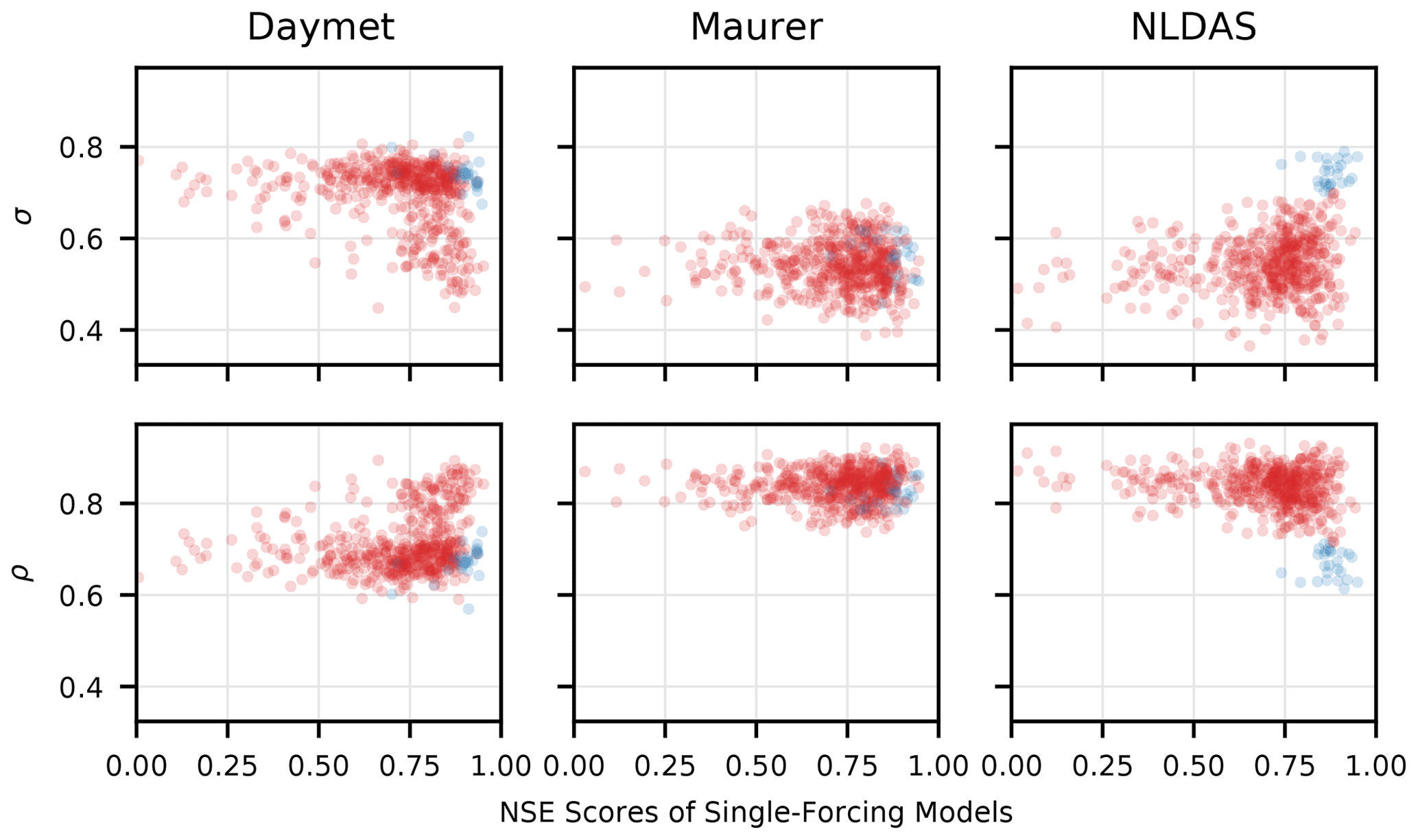
Figure C2As in Fig. C1, the triple collocation error variances (σ – Eq. C4) and truth correlations (ρ – Eq. C5) are plotted against NSE scores of the single-forcing LSTM models. The coloring shows the anomalous NLDAS basins in blue and all others in red. For these basins, NLDAS has low correlation with the other two products but still yields high-skill simulations.

Figure C3Spatial distribution of anomalous NLDAS basins shown in Fig. C2 (a) compared with elevation of the CAMELS basins (b).
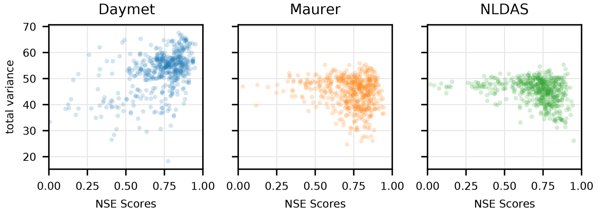
Figure C4Performance of single-input models relative to the total variance of log precipitation in each basin. The Daymet model tends to perform better in wetter basins (as the total Daymet variance increases), but the other two products have poor-performing basins in catchments with high precipitation variance.
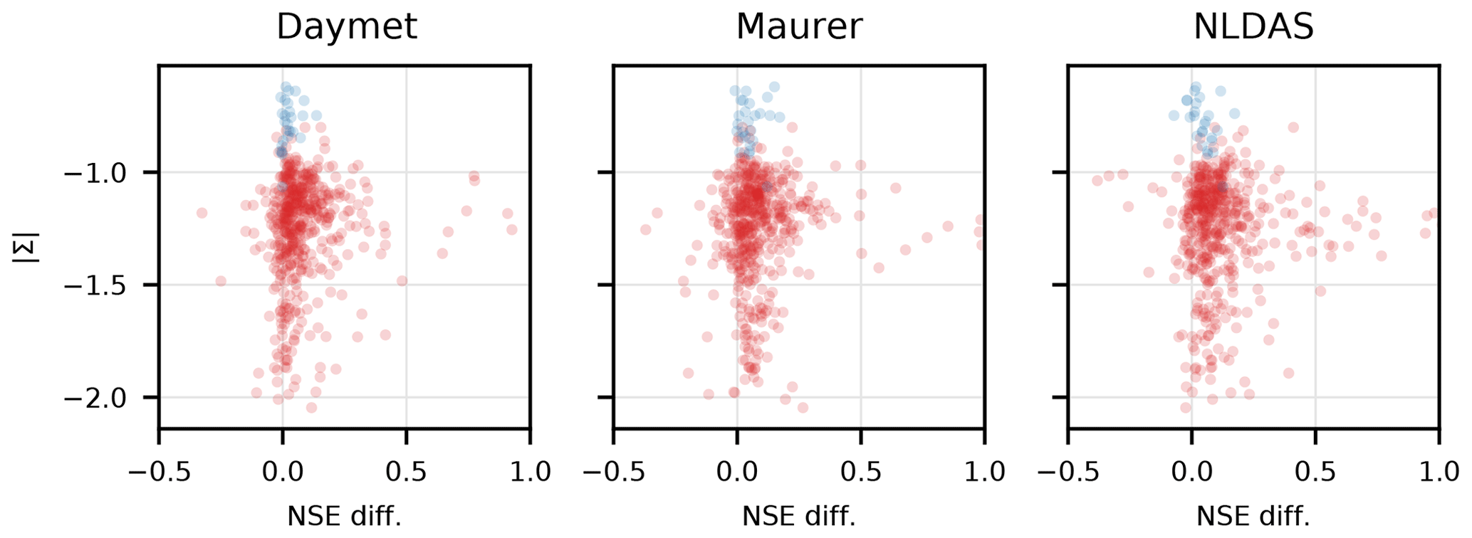
Figure C5Fractional increase in NSE from the three-forcing model relative to the single-forcing models plotted against the log determinant of the covariance matrix of all three (standardized, log-transformed) precipitation products (). increases when there is a larger disagreement between the three data sets, approximating the joint entropy of the three products. With the exception of the anomalous NLDAS basins (blue markers), the three-forcing model offers improvements with respect to the single-forcing models when there is larger disagreement between the three data sets. The three-forcing model learned to leverage synergy in these three precipitation products.
Figure C4 plots model performance against the individual variances of the precipitation products in each basin. This figure shows that the single-forcing Daymet LSTM tended to perform better in catchments with higher total precipitation variance (not triple collocation error variance). This is, again, not true for the other two models, where higher total variance was associated with a higher variance in model skill, indicating that a higher proportion of the total variance is likely due to measurement error.
To analyze the synergy due to using all forcings in a single LSTM, we transposed the NSE improvements in each basin (due to using all three forcing products in the same LSTM) with the log determinant of the covariance matrix of all three (standardized, log-transformed) precipitation products (Fig. C5). The log determinant is a proxy for the joint entropy of the three (standardized, log-transformed) products and increases when there is larger disagreement between the three data sets. Unlike in Fig. C4, the variances in Fig. C5 were calculated after removing the mean and overall variance of each log-transformed precipitation product so that the log determinant of the covariance is not affected by the overall magnitude of precipitation in each catchment (i.e., does not increase in wetter catchments). With the exception of the anomalous NLDAS basins, Fig. C5 shows that the three-forcing model offered improvements with respect to the single-forcing models when there was larger disagreement between the three data sets. This indicates that there is value in diversity among precipitation data sets and that the LSTM can exploit this diversity.
The code required to reproduce all LSTM results and figures is available at https://doi.org/10.5281/zenodo.4738770. The code for running and optimizing SAC-SMA is available from the “multi-inputs” branch at the following repository: https://github.com/Upstream-Tech/SACSMA-SNOW17.git (Upstream-Tech, 2020).
The validation periods of all benchmark models used in this study are available at https://doi.org/10.4211/hs.474ecc37e7db45baa425cdb4fc1b61e1 (Kratzert et al., 2019c). The extended Maurer forcings, including daily minimum and maximum temperature, are available at https://doi.org/10.4211/hs.17c896843cf940339c3c3496d0c1c077 (Kratzert, 2019b). The extended NLDAS forcings, including daily minimum and maximum temperature, are available at https://doi.org/10.4211/hs.0a68bfd7ddf642a8be9041d60f40868c (Kratzert, 2019a). Finally, the weights of the pre-trained models are available at https://doi.org/10.5281/zenodo.4670268 (Kratzert et al., 2021).
FK had the idea to train LSTMs on multiple forcing products. FK, DK, and GSN designed all the experiments. FK trained the models and evaluated the results. GSN did the triple collocation analysis and the integrated gradients analysis. GSN supervised the paper from the hydrological perspective and SH from the machine learning perspective. GSN and SH shared the responsibility of the last authorship in their respective fields. All authors worked on the paper.
The authors declare that they have no conflict of interest.
Authors from the Johannes Kepler University acknowledge support from Bosch, ZF, Google (Faculty Research Award), the NVIDIA Corporation, GPU donations, LIT (grant no. LIT-2017-3-YOU-003), and FWF (grant no. P 28660-N31). Grey Nearing acknowledges support from the NASA Advanced Information Systems Technology program (award ID 80NSSC17K0541).
The project relies heavily on open-source software. All programming was done in Python version 3.7 (van Rossum, 1995) and the associated libraries, including NumPy (Van Der Walt et al., 2011), Pandas (McKinney, 2010), PyTorch (Paszke et al., 2017), SciPy (Virtanen et al., 2020), Matplotlib (Hunter, 2007), xarray (Hoyer and Hamman, 2017), and SPOTPY (Houska et al., 2019).
This research has been supported by the Global Water Futures project, the Bundesministerium für Bildung, Wissenschaft und Forschung (grant nos. LIT-2018-6-YOU-212, LIT-2017-3-YOU-003, LIT-2018-6-YOU-214, and LIT-2019-8-YOU-213), the Österreichische Forschungsförderungsgesellschaft (grant nos. FFG-873979, FFG-872172, and FFG-871302), the European Commission's Horizon 2020 Framework Programme (AIDD; grant no. 956832), Janssen Pharmaceuticals, UCB Biopharma SRL, Merck Healthcare KGaA, the Audi.JKU Deep Learning Center, TGW Logistics Group GmbH, Silicon Austria Labs (SAL), FILL Gesellschaft mbH, Anyline GmbH, Google, ZF Friedrichshafen AG, Robert Bosch GmbH, Software Competence Center Hagenberg GmbH, TÜV Austria, NVIDIA Corporation, and Microsoft Canada.
This paper was edited by Dimitri Solomatine and reviewed by Thomas Lees and two anonymous referees.
Addor, N., Newman, A. J., Mizukami, N., and Clark, M. P.: The CAMELS data set: catchment attributes and meteorology for large-sample studies, Hydrol. Earth Syst. Sci., 21, 5293–5313, https://doi.org/10.5194/hess-21-5293-2017, 2017a. a
Addor, N., Newman, A. J., Mizukami, N., and Clark, M. P.: Catchment attributes for large-sample studies, Boulder, CO, UCAR/NCAR, https://doi.org/10.5065/D6G73C3Q, 2017b. a
Addor, N., Nearing, G., Prieto, C., Newman, A. J., Le Vine, N., and Clark, M. P.: A Ranking of Hydrological Signatures Based on Their Predictability in Space, Water Resour. Res., 54, 8792–8812, https://doi.org/10.1029/2018WR022606, 2018. a, b
Alemohammad, S. H., McColl, K. A., Konings, A. G., Entekhabi, D., and Stoffelen, A.: Characterization of precipitation product errors across the United States using multiplicative triple collocation, Hydrol. Earth Syst. Sci., 19, 3489–3503, https://doi.org/10.5194/hess-19-3489-2015, 2015. a
Beck, H. E., Vergopolan, N., Pan, M., Levizzani, V., van Dijk, A. I. J. M., Weedon, G. P., Brocca, L., Pappenberger, F., Huffman, G. J., and Wood, E. F.: Global-scale evaluation of 22 precipitation datasets using gauge observations and hydrological modeling, Hydrol. Earth Syst. Sci., 21, 6201–6217, https://doi.org/10.5194/hess-21-6201-2017, 2017. a
Behnke, R., Vavrus, S., Allstadt, A., Albright, T., Thogmartin, W. E., and Radeloff, V. C.: Evaluation of downscaled, gridded climate data for the conterminous United States, Ecol. Appl., 26, 1338–1351, 2016. a, b, c, d, e, f
Clark, M. P., Wilby, R. L., Gutmann, E. D., Vano, J. A., Gangopadhyay, S., Wood, A. W., Fowler, H. J., Prudhomme, C., Arnold, J. R., and Brekke, L. D.: Characterizing uncertainty of the hydrologic impacts of climate change, Current Climate Change Reports, 2, 55–64, 2016. a, b, c
Clausen, B. and Biggs, B.: Flow variables for ecological studies in temperate streams: groupings based on covariance, J. Hydrol., 237, 184–197, https://doi.org/10.1016/S0022-1694(00)00306-1, 2000. a, b
Court, A.: Measures of streamflow timing, J. Geophys. Res., 67, 4335–4339, https://doi.org/10.1029/JZ067i011p04335, 1962. a
Duan, Q., Ajami, N. K., Gao, X., and Sorooshian, S.: Multi-model ensemble hydrologic prediction using Bayesian model averaging, Adv. Water Resour., 30, 1371–1386, 2007. a
Frame, J., Nearing, G., Kratzert, F., and Rahman, M.: Post processing the US National Water Model with a Long Short-Term Memory network, J. Am. Water Resour. As., https://doi.org/10.31223/osf.io/4xhac, in review, 2020. a
Gers, F. A., Schmidhuber, J., and Cummins, F.: Learning to forget: continual prediction with LSTM, Neural Comput., 12, 2451–2471, 2000. a
Gupta, H. V., Kling, H., Yilmaz, K. K., and Martinez, G. F.: Decomposition of the mean squared error and NSE performance criteria: Implications for improving hydrological modelling, J. Hydrol., 377, 80–91, 2009. a, b, c
Henn, B., Newman, A. J., Livneh, B., Daly, C., and Lundquist, J. D.: An assessment of differences in gridded precipitation datasets in complex terrain, J. Hydrol., 556, 1205–1219, 2018. a
Hochreiter, S.: Untersuchungen zu dynamischen neuronalen Netzen, Diploma, Technische Universität München, München, 91, 1991. a
Hochreiter, S. and Schmidhuber, J.: Flat minima, Neural Comput., 9, 1–42, 1997a. a
Hochreiter, S. and Schmidhuber, J.: Long short-term memory, Neural Comput., 9, 1735–1780, 1997b. a
Houska, T., Kraft, P., Chamorro-Chavez, A. and Breuer, L.: SPOTting Model Parameters Using a Ready-Made Python Package, PLoS ONE, 10, e0145180, https://doi.org/10.1371/journal.pone.0145180, 2015. a, b
Hoyer, S. and Hamman, J.: xarray: N-D labeled arrays and datasets in Python, Journal of Open Research Software, 5, p. 10, https://doi.org/10.5334/jors.148, 2017. a
Hunter, J. D.: Matplotlib: A 2D graphics environment, Comput. Sci. Eng., 9, 90–95, 2007. a
Kingma, D. P. and Ba, J.: Adam: A method for stochastic optimization, arXiv [preprint], arXiv:1412.6980, 2014. a
Kratzert, F.: Extended NLDAS forcings, HydroShare, https://doi.org/10.4211/hs.0a68bfd7ddf642a8be9041d60f40868c, 2019. a
Kratzert, F.: Extended Maurer forcings, HydroShare, https://doi.org/10.4211/hs.17c896843cf940339c3c3496d0c1c077, 2019b. a
Kratzert, F., Klotz, D., Brenner, C., Schulz, K., and Herrnegger, M.: Rainfall–runoff modelling using Long Short-Term Memory (LSTM) networks, Hydrol. Earth Syst. Sci., 22, 6005–6022, https://doi.org/10.5194/hess-22-6005-2018, 2018. a
Kratzert, F., Klotz, D., Herrnegger, M., Sampson, A. K., Hochreiter, S., and Nearing, G. S.: Toward Improved Predictions in Ungauged Basins: Exploiting the Power of Machine Learning, Water Resour. Res., 55, 11344–11354, https://doi.org/10.1029/2019WR026065, 2019a. a, b, c, d
Kratzert, F., Klotz, D., Shalev, G., Klambauer, G., Hochreiter, S., and Nearing, G.: Towards learning universal, regional, and local hydrological behaviors via machine learning applied to large-sample datasets, Hydrol. Earth Syst. Sci., 23, 5089–5110, https://doi.org/10.5194/hess-23-5089-2019, 2019b. a, b, c, d, e, f, g
Kratzert, F., Klotz, D., Hochreiter, S., and Nearing, G. S.: Benchmark models, HydroShare, https://doi.org/10.4211/hs.474ecc37e7db45baa425cdb4fc1b61e1, 2019c. a
Kratzert, F., Klotz, D., Hochreiter, S., and Nearing, G. S.: Pre-trained models, Zenodo [data set], https://doi.org/10.5281/zenodo.4670268, 2021. a
Ladson, A., Brown, R., Neal, B., and Nathan, R.: A standard approach to baseflow separation using the Lyne and Hollick filter, Australian Journal of Water Resources, 17, , 25–34, 2013. a
Lundquist, J., Hughes, M., Gutmann, E., and Kapnick, S.: Our skill in modeling mountain rain and snow is bypassing the skill of our observational networks, B. Am. Meteorol. Soc., 100, 2473–2490, https://doi.org/10.1175/BAMS-D-19-0001.1, 2019. a
Madadgar, S. and Moradkhani, H.: Improved B ayesian multimodeling: Integration of copulas and B ayesian model averaging, Water Resour. Res., 50, 9586–9603, 2014. a
Maurer, E. P., Wood, A., Adam, J., Lettenmaier, D. P., and Nijssen, B.: A long-term hydrologically based dataset of land surface fluxes and states for the conterminous United States, J. Climate, 15, 3237–3251, 2002. a
McColl, K. A., Vogelzang, J., Konings, A. G., Entekhabi, D., Piles, M., and Stoffelen, A.: Extended triple collocation: Estimating errors and correlation coefficients with respect to an unknown target: EXTENDED TRIPLE COLLOCATION, Geophys. Res. Lett., 41, 6229–6236, https://doi.org/10.1002/2014GL061322, 2014. a
McKinney, W.: Data Structures for Statistical Computing in Python, Proceedings of the 9th Python in Science Conference, Austin, Texas, 28 June–3 July, 1697900, 51–56, 2010. a
Nash, J. E. and Sutcliffe, J. V.: River flow forecasting through conceptual models part I – A discussion of principles, J. Hydrol., 10, 282–290, 1970. a
Newman, A., Sampson, K., Clark, M., Bock, A., Viger, R., and Blodgett, D.: A large-sample watershed-scale hydrometeorological dataset for the contiguous USA, Boulder, CO: UCAR/NCAR, https://doi.org/10.5065/D6MW2F4D, 2014. a, b
Newman, A. J., Mizukami, N., Clark, M. P., Wood, A. W., Nijssen, B., and Nearing, G.: Benchmarking of a physically based hydrologic model, J. Hydrometeorol., 18, 2215–2225, 2017. a, b, c, d, e
Newman, A. J., Clark, M. P., Longman, R. J., and Giambelluca, T. W.: Methodological intercomparisons of station-based gridded meteorological products: Utility, limitations, and paths forward, J. Hydrometeorol., 20, 531–547, 2019. a
Olden, J. D. and Poff, N. L.: Redundancy and the choice of hydrologic indices for characterizing streamflow regimes, River Res. Appl., 19, 101–121, https://doi.org/10.1002/rra.700, 2003. a, b
Parkes, B., Higginbottom, T. P., Hufkens, K., Ceballos, F., Kramer, B., and Foster, T.: Weather dataset choice introduces uncertainty to estimates of crop yield responses to climate variability and change, Environ. Res. Lett., 14, 124089, https://doi.org/10.1088/1748-9326/ab5ebb, 2019. a
Paszke, A., Gross, S., Chintala, S., Chanan, G., Yang, E., DeVito, Z., Lin, Z., Desmaison, A., Antiga, L., and Lerer, A.: Pytorch: an imperative style, high-performance deep learning library,in: Advances in Neural Information Processing Systems, 32, 8024–8035, 2017. a
Pearl, J.: Embracing causality in default reasoning, Artificial Intelligence, 35, 259–271, 1988. a
Sankarasubramanian, A., Vogel, R. M., and Limbrunner, J. F.: Climate elasticity of streamflow in the United States, Water Resour. Res., 37, 1771–1781, https://doi.org/10.1029/2000WR900330, 2001. a
Sawicz, K., Wagener, T., Sivapalan, M., Troch, P. A., and Carrillo, G.: Catchment classification: empirical analysis of hydrologic similarity based on catchment function in the eastern USA, Hydrol. Earth Syst. Sci., 15, 2895–2911, https://doi.org/10.5194/hess-15-2895-2011, 2011. a, b
Scipal, K., Dorigo, W., and deJeu, R.: Triple collocation—A new tool to determine the error structure of global soil moisture products, in: 2010 IEEE International Geoscience and Remote Sensing Symposium, Honolulu, HI, USA, 25—30 July 2010, 4426–4429, IEEE, 2010. a
Shrikumar, A., Greenside, P., Shcherbina, A., and Kundaje, A.: Not just a black box: Learning important features through propagating activation differences, arXiv [preprint], arXiv:1605.01713, 2016. a
Stoffelen, A.: Toward the true near-surface wind speed: Error modeling and calibration using triple collocation, J. Geophys. Res.-Oceans, 103, 7755–7766, 1998. a
Sundararajan, M., Taly, A., and Yan, Q.: Axiomatic attribution for deep networks, in: Proceedings of the 34th International Conference on Machine Learning-Volume 70, 3319–3328, available at: http://proceedings.mlr.press/v70/sundararajan17a.html (last access: 13 May 2020), 2017. a, b, c
Sutton, R.: The bitter lesson, Incomplete Ideas (blog), available at: http://www.incompleteideas.net/IncIdeas/BitterLesson.html (last access: 13 May 2020), 2019. a
Thornton, P. E., Running, S. W., White, M. A.: Generating surfaces of daily meteorological variables over large regions of complex terrain, J. Hydrol., 190, 214–251, 1997. a
Timmermans, B., Wehner, M., Cooley, D., O'Brien, T., and Krishnan, H.: An evaluation of the consistency of extremes in gridded precipitation data sets, Clim. Dynam., 52, 6651–6670, 2019. a
Upstream-Tech: SACSMA-SNOW17, available at: https://github.com/Upstream-Tech/SACSMA-SNOW17.git, last access: 11 July 2020. a
Tolson, B. A. and Shoemaker, C. A.: Dynamically dimensioned search algorithm for computationally efficient watershed model calibration, Water Resour. Res., 43, W01413, https://doi.org/10.1029/2005WR004723, 2007. a
Van Der Walt, S., Colbert, S. C., and Varoquaux, G.: The NumPy array: A structure for efficient numerical computation, Comput. Sci. Eng., 13, 22–30, 2011. a
van Rossum, G.: Python tutorial, Technical Report CS-R9526, Tech. rep., Centrum voor Wiskunde en Informatica (CWI), Amsterdam, 1995. a
Virtanen, P., Gommers, R., Oliphant, T. E., Haberland, M., Reddy, T., Cournapeau, D., Burovski, E., Peterson, P., Weckesser, W., Bright, J., van der Walt, S. J., Brett, M., Wilson, J., Jarrod Millman, K., Mayorov, N., Nelson, A. R. J., Jones, E., Kern, R., Larson, E., Carey, C., Polat, İ., Feng, Y., Moore, E. W., Vand erPlas, J., Laxalde, D., Perktold, J., Cimrman, R., Henriksen, I., Quintero, E. A., Harris, C. R., Archibald, A. M., Ribeiro, A. H., Pedregosa, F., van Mulbregt, P., and Contributors, S. . .: SciPy 1.0: Fundamental Algorithms for Scientific Computing in Python, Nat. Methods, 17, 261–272, https://doi.org/10.1038/s41592-019-0686-2, 2020. a, b
Wellman, M. P. and Henrion, M.: Explaining'explaining away', IEEE T. Pattern Anal., 15, 287–292, 1993. a
Westerberg, I. K. and McMillan, H. K.: Uncertainty in hydrological signatures, Hydrol. Earth Syst. Sci., 19, 3951–3968, https://doi.org/10.5194/hess-19-3951-2015, 2015. a, b, c, d
Xia, Y., Mitchell, K., Ek, M., Sheffield, J., Cosgrove, B., Wood, E., Luo, L., Alonge, C., Wei, H., Meng, J., Livneh, B., Lettenmaier, D., Koren, V., Duan, Q., Mo, K., Fan, Y., and Mocko, D.: Continental-scale water and energy flux analysis and validation for the North American Land Data Assimilation System project phase 2 (NLDAS-2): 1. Intercomparison and application of model products, J. Geophys. Res.-Atmos., 117, D03109, https://doi.org/10.1029/2011JD016048, 2012. a
Yilmaz, K. K., Hogue, T. S., Hsu, K.-L., Sorooshian, S., Gupta, H. V., and Wagener, T.: Intercomparison of rain gauge, radar, and satellite-based precipitation estimates with emphasis on hydrologic forecasting, J. Hydrometeorol., 6, 497–517, 2005. a
Yilmaz, K. K., Gupta, H. V., and Wagener, T.: A process-based diagnostic approach to model evaluation: Application to the NWS distributed hydrologic model, Water Resour. Res., 44, W09417, https://doi.org/10.1029/2007WR006716, 2008. a, b, c
- Abstract
- Introduction
- Methods
- Results and discussion
- Conclusions
- Appendix A: Average LSTM single-model performance
- Appendix B: Peak flow timing
- Appendix C: Analysis of precipitation uncertainty
- Code availability
- Data availability
- Author contributions
- Competing interests
- Acknowledgements
- Financial support
- Review statement
- References