Model representation of the coupling between evapotranspiration and soil water content at different depths

Soil water content (θ) influences the climate system by controlling the fraction of incoming solar and longwave energy that is converted into evapotranspiration (ET). Therefore, investigating the coupling strength between θ and ET is important for the study of land surface–atmosphere interactions. Physical models are commonly tasked with representing the coupling between θ and ET; however, few studies have evaluated the accuracy of model-based estimates of θ ∕ ET coupling (especially at multiple soil depths). To address this issue, we use in situ AmeriFlux observations to evaluate θ ∕ ET coupling strength estimates acquired from multiple land surface models (LSMs) and an ET retrieval algorithm – the Global Land Evaporation Amsterdam Model (GLEAM). For maximum robustness, coupling strength is represented using the sampled normalized mutual information (NMI) between θ estimates acquired at various vertical depths and surface evaporation flux expressed as a fraction of potential evapotranspiration (fPET, the ratio of ET to potential ET). Results indicate that LSMs and GLEAM are generally in agreement with AmeriFlux measurements in that surface soil water content (θ_s) contains slightly more NMI with fPET than vertically integrated soil water content (θ_v). Overall, LSMs and GLEAM adequately capture variations in NMI between fPET and θ estimates acquired at various vertical depths. However, GLEAM significantly overestimates the NMI between θ and ET, and the relative contribution of θ_s to total ET. This bias appears attributable to differences in GLEAM's ET estimation scheme relative to the other two LSMs considered here (i.e., the Noah model with multi-parameterization options and the Catchment Land Surface Model, CLSM). These results provide insight into improved LSM model structure and parameter optimization for land surface–atmosphere coupling analyses.

1 Introduction

Soil water content (θ) modulates water and energy feedbacks between the land surface and the lower atmosphere by determining the fraction of incoming solar energy that is converted into evapotranspiration (ET; Seneviratne et al., 2010, 2013). In water-limited regimes, θ exhibits a dominant control on ET, and therefore exerts significant terrestrial control on the Earth's water and energy cycles. Accurately representing θ ∕ ET coupling in land surface models (LSMs) is therefore expected to improve our ability to project the future frequency of extreme climates (Seneviratne et al., 2013).

A key question is how the constraint of θ on ET and sensible heat (H) varies as θ is vertically integrated over deeper vertical soil depths. Given the tendency for the timescales of θ dynamics to vary strongly with depth, the degree to which the ET is coupled with vertical variations in θ determines the temporal scale at which θ variations are propagated into the lower atmosphere. Therefore, in order to represent θ ∕ ET coupling, and thus land–atmosphere interactions in general, LSMs must accurately capture the relationship between vertically varying θ values and ET. Unfortunately, their ability to do so remains an open question.

Recently, land surface–atmosphere coupling strength has been investigated by sampling mutual information proxies (e.g., correlation coefficient or other coupling indices) between time series of θ and ET observations (or air temperature proxies for ET). Results suggest that, even when confined to very limited vertical support (e.g., within the top 5 cm of the soil column), surface θ estimates retain significant information for describing overall θ control on local climate (Ford and Quiring, 2014; Qiu et al., 2014; Dong and Crow, 2018, 2019). These findings are in contrast with the common perception that ET is constrained only by θ values within deeper soil layers (Hirschi et al., 2014). Hence, it is necessary to examine whether LSMs can realistically reflect observed variations of θ ∕ ET coupling strength within the vertical soil profile.

Previous studies examining the θ ∕ ET relationship have generally been based on Pearson product–moment correlation (Basara and Crawford, 2002; Ford et al., 2014), which captures only the strength of a linear relationship between two variables. However, the coupling between θ and ET is generally nonlinear. Therefore, non-parametric mutual information measures are generally more appropriate. Nearing et al. (2018) used information theory metrics (transfer entropy, in particular) to measure the strength of direct couplings between different surface variables, including soil water content, and surface energy fluxes at short timescales in several LSMs. They found that the LSMs are generally biased as compared with the strengths of couplings in observation data, and that these biases differ across different study sites. However, they did not look specifically at the effect of vertical water content profiles or of subsurface soil water content on partitioning surface energy fluxes.

Here we apply the information theory-based methodology of Qiu et al. (2016) to examine the relationship between the vertical support of θ estimates and their mutual information (MI) with respect to ET. Our approach is based on analyzing the MI content between ET and θ time series acquired from both LSMs, and ET retrieval algorithm – the Global Land Evaporation Amsterdam Model (GLEAM) – and AmeriFlux in situ observations. MI values are then normalized by entropy in the corresponding ET time series to remove the effect of inter-site variations to generate estimates of normalized mutual information (NMI) between θ and ET. Both surface (roughly 0–10 cm) soil water content (θ_s) and vertically integrated (0–40 cm) soil water content (θ_v) are considered to capture the impact of depth on NMI results. AmeriFlux-based NMI results are then compared with analogous NMI results obtained from LSM-based and GLEAM-based θ and ET time series.

2 Data and methods

The AmeriFlux network provides temporally continuous measurements of θ, surface energy fluxes and related environmental variables for sites located in a variety of North American ecosystem types, e.g., forests, grasslands, croplands, shrublands and savannas (Boden et al., 2013). To minimize sampling errors, AmeriFlux sites lacking a complete 3-year summer months (June, July and August) daily time series between the years of 2003 and 2015 (i.e., $\mathrm{3}\times \mathrm{92}=\mathrm{276}$ daily observations in total) of θ_s, θ_v and latent heat flux (LE) are excluded here, resulting in the 34 remaining eligible AmeriFlux sites listed in Table 1. These sites cover a variety of climate zones within the contiguous United States (CONUS). Table 1 gives background information on these 34 sites including local land-cover information. Hydro-climatic conditions in each site are characterized using the aridity index (AI), calculated using CRU (Climate Research Unit, v4.02) monthly precipitation and potential evaporation (PET) datasets.

As described above, θ ∕ ET coupling assessments made using AmeriFlux observations are compared with those using state-of-the-art LSMs including the Noah model with multi-parameterization options (NOAHMP) and Catchment Land Surface Model (CLSM). In addition, θ and ET retrievals provided by the Global Land Evaporation Amsterdam Model (GLEAM) are also considered. See below for details on all three approaches. To avoid any spurious correlations between θ and ET due to seasonality, all NMI analyses are performed on θ and ET time series anomalies acquired during the period 2003–2015. The θ and ET anomalies are calculated by removing the seasonal cycle – defined as 31 d window averages centered on each day of the year sampled across all years of the 2003–2015 historical data record – from the raw θ and ET time series data. The analysis is limited to the CONUS during summer months (June, July and August) when θ ∕ ET coupling is expected to be maximized.

Table 1 Attributes of selected AmeriFlux sites.

^a Was 5 cm prior to 13 April 2005. ^b Was 25 cm prior to 13 April 2005. ^c Was 5 cm prior to 1 January 2006. ^d Was 0–30 cm prior to 2007. ^e Unavailable prior to 2007. NA = not available.

2.1 Ground-based AmeriFlux measurements

The Level 2 (L2) AmeriFlux LE and H flux observations are based on high-frequency (typically > 10 Hz) eddy covariance measurements processed into half-hourly averages by individual AmeriFlux investigators. LE and θ observations at a half-hour time step and without gap-filling procedures are collected from the AmeriFlux Site and Data Exploration System (see http://ameriflux.ornl.gov/, last access: November 2018). The LE and θ observations are further aggregated into daily (00:00 to 24:00 UTC) values, and daily LE is converted into daily ET using the latent heat of vaporization. Daily ET values based on less than 30 % half-hourly coverage (i.e., < 15 half-hourly observations per day) are considered not representative at a daily timescale and are therefore excluded.

Soil water content measurements are generally available at two discrete depths that vary between the AmeriFlux sites (Table 1). Here, the top (i.e., closest to the surface) soil water content observation is always used to represent surface soil water content (θ_s). Since the depth of this top-layer measurement varies between 0 and 15 cm (see Table 1), we consider the surface-layer measurement θ_s to be roughly representative of 0–10 cm (vertically integrated) θ. For more details on AmeriFlux sites utilized here, see Raz-Yaseef et al. (2015).

Given variations in the depth of the lower AmeriFlux θ observations (see Table 1), we applied a variety of approaches for estimating vertically integrated soil water content (θ_v). Our first approach, hereinafter referred to as Case I, is based on the application of an exponential filter (Wagner et al., 1999; Albergel et al., 2008) to extrapolate θ_s to a consistent 40 cm bottom-layer depth. Therefore, only θ_s is used to derive θ_v and the bottom-layer (or second-layer) AmeriFlux θ measurement is neglected in this case. The application of the exponential filter requires a single timescale parameter T. Since θ measurements from the United States Department of Agriculture's Soil Climate Analysis Network (SCAN) are taken at fixed soil depth, we utilized this dataset to determine the most appropriate parameter T at AmeriFlux sites. Following Qiu et al. (2014), first, we estimated the optimal parameter T (T_opt) for the extrapolation of θ measurements from 10 to 40 cm depth and established a global relationship between Topt and site-based NDVI (MOD13Q1 v006, 250 m, 16 d; $T_{\mathrm{opt}}=\mathrm{2.098}\times \exp (-\mathrm{1.895}\times$ (NDVI +0.6271)) +2.766). Then, this global relationship (goodness of fit R²: 0.85) is applied to AmeriFlux sites to extrapolate 0–10 cm θ_s time series into 0–40 cm θ_v.

Previous research has suggested that such a filtering approach does not significantly squander ET information present in actual measurements of θ_v (Qiu et al., 2014, 2016). Nevertheless, since the quality of θ_v estimates is important in our analysis, we also calculated two additional cases where 0–40 cm θ_v is estimated using (1) the bottom-layer soil water content measurement acquired at each AmeriFlux site (hereinafter, Case II) and (2) linear interpolation of θ_s, and the bottom-layer AmeriFlux soil water content measurement (hereinafter, Case III). The sensitivity of key results to these various cases is discussed below.

2.2 LSM- and GLEAM-based simulations

Simulations are acquired from the NOAHMP (Niu et al., 2011) and CLSM (Koster et al., 2000) LSMs embedded within the NASA Land Information System (LIS, Kumar et al., 2006) and the GLEAM ET retrieval algorithm (Miralles et al., 2011). Both NOAHMP and CLSM are set up to simulate 0.125^∘ θ profiles at a 15 min time step using North America Land Data Assimilation System, Phase 2 (NLDAS-2) forcing data. A 10-year model spin-up period (1992 to 2002) is applied for NOAHMP and CLSM.

NOAHMP numerically solves the one-dimensional Richards equation within four soil layers of thicknesses of 0–10, 11–30, 31–60 and 61–100 cm. Major parameterization options relevant to θ simulation include options for canopy stomatal resistance parameterization and schemes controlling the effect of θ on the vegetation stress factor β. Here we employed the Ball–Berry-type stomatal resistance scheme and Noah-type soil water content factor controlling the β factor. The specific expressions are as follows:

$$\begin{array}{}\text{(1)}& \mathit{\beta }={\sum }_{i=\mathrm{1}}^{N_{\mathrm{root}}}{\displaystyle \frac{\mathrm{\Delta }{Z}_i}{Z_{\mathrm{root}}}}min\left(\mathrm{1.0},{\displaystyle \frac{{\mathit{\theta }}_i-{\mathit{\theta }}_{\mathrm{wilt}}}{{\mathit{\theta }}_{\mathrm{ref}}-{\mathit{\theta }}_{\mathrm{wilt}}}},\right)\end{array}$$

where θ_wilt and θ_ref are, respectively, soil water content at the wilting point (m³ m⁻³) and reference soil water content (m³ m⁻³), which is set as field capacity during parameterization. θ_i and Δz_i are soil water content (m³ m⁻³) and soil depth (cm) at ith layer, N_root and z_root are total number of soil layers with roots and total depth (cm) of root zone, respectively.

Following the Ball–Berry stomatal resistance scheme, the θ-controlled β factor and other multiplicative factors including temperature and foliage nitrogen simultaneously determine the maximum carboxylation rate V_max as follows:

$$\begin{array}{}\text{(2)}& V_{\max }=V_{\max \mathrm{25}}{\mathit{\alpha }}_{\mathrm{vmax}}^{\frac{T_{\mathrm{v}}-\mathrm{25}}{\mathrm{10}}}f\left(N\right)f\left(T_{\mathrm{v}}\right)\mathit{\beta },\end{array}$$

where V_max25 is maximum carboxylation rate at 25 ^∘C (µmol CO₂ m⁻² s⁻¹), α_vmax is a parameter sensitive to vegetation canopy surface temperature T_v, f(N) is a factor representing foliage nitrogen and f(T_v) is a function that mimics thermal breakdown of metabolic processes. Based on V_max, photosynthesis rates per unit leaf area index (LAI) including carboxylase-limited (Rubisco limited, denoted by A_C) type and export-limited (for C₃ plants, denoted by A_S) type are calculated, respectively. The minimum of A_C, A_S and the light-limited photosynthesis rate determines stomatal resistance r_s, and consequently affects ET over vegetated areas. For the complete NOAHMP configuration, please see Table S1 in the Supplement.

CLSM simulates the 0–2 and 0–100 cm soil water content and evaporative stress as a function of simulated θ and environmental variables. ET is then estimated based on the estimated evaporative stress and land–atmosphere humidity gradients. Energy and water flux estimates are iterated with soil state estimates (e.g., θ and soil temperature) to ensure closure of surface energy and water balances. For a detailed explanation of CLSM physics, please refer to Koster et al. (2000).

GLEAM is a set of algorithms dedicated to the estimation of terrestrial ET and root-zone θ from satellite data. In this study, the latest version of this model (v3.2a) is employed. In GLEAM, the configuration of soil layers varies as a function of the land-cover type. Soil stratification is based on three soil layers for tall vegetation (0–10, 10–100 and 100–250 cm), two layers for low vegetation (0–10 and 10–100 cm) and only one layer for bare soil (0–10 cm; Martens et al., 2017).

The cover-dependent PET (mm d⁻¹) of GLEAM is calculated using the Priestley and Taylor (1972) equation based on observed air temperature and net radiation. Following this, estimates of PET are converted into actual transpiration or bare soil evaporation (depending on the land-cover type, ET (mm d⁻¹)), using a cover-dependent, multiplicative stress factor S (–), which is calculated as a function of microwave vegetation optical depth (VOD) and root-zone θ (Miralles et al., 2011). The related expressions are as follows:

$$\begin{array}{}\text{(3)}& {\displaystyle }\mathrm{ET}=\mathrm{PET}\times S+E_{\mathrm{i}},\text{(4)}& {\displaystyle }S=\sqrt{{\displaystyle \frac{\mathrm{VOD}}{{\mathrm{VOD}}_{\max }}}}\left(\mathrm{1}-{\left({\displaystyle \frac{{\mathit{\theta }}_{\mathrm{c}}-\mathit{\theta }\mathit{\omega }}{{\mathit{\theta }}_{\mathrm{c}}-{\mathit{\theta }}_{\mathrm{wilt}}}}\right)}^{\mathrm{2}}\right),\end{array}$$

where E_i is rainfall interception (mm), S essentially represents the fPET (see Sect. 2.3) estimated by GLEAM, θ_c (m³ m⁻³) is the critical soil water content and θω (m³ m⁻³) is the soil water content of the wettest layer, assuming that plants withdraw water from the layer that is most accessible. Based on Eq. (4), GLEAM S (or fPET) tends to become more sensitive to θ in areas of low VOD seasonality (i.e., low differences between VOD and VOD_max). As for bare soil conditions, S is linearly related to surface soil water content (θ₁):

$$\begin{array}{}\text{(5)}& S=\mathrm{1}-{\displaystyle \frac{{\mathit{\theta }}_{\mathrm{c}}-{\mathit{\theta }}_{\mathrm{1}}}{{\mathit{\theta }}_{\mathrm{c}}-{\mathit{\theta }}_{\mathrm{wilt}}}}.\end{array}$$

To resolve variations in the vertical discretization of θ applied by each model, we linearly interpolated NOAHMP, CLSM and GLEAM outputs into daily 0–10 and 0–40 cm soil water content values using depth-weighted averaging.

2.3 Variable indicating soil water content and surface flux coupling

Soil water content–ET coupling can be diagnosed using a variety of different variables derived from ET, e.g., the fraction of PET (fPET, the ratio of ET and PET) or the evaporative fraction (EF, the ratio of LE and the sum of LE and sensible heat). Since ET is strongly tied to net radiation (R_n; Koster et al., 2009), both fPET and EF are advantageous in that they normalize ET by removing the impact of non-soil water content influences on ET (e.g., net radiation, wind speed and soil heat flux (G)). However, since sensible heat flux is not provided in the GLEAM dataset, we are restricted here to using fPET.

It should be noted that the applied meteorological forcing data for NOAHMP and CLSM are somewhat different from those used for GLEAM. Therefore, to minimize the impact of this difference, NOAHMP and CLSM fPET are computed from North American Regional Reanalysis (NARR) using the modified Penman scheme of Mahrt and Ek (1984), while GLEAM fPET is calculated using its own internal PET estimates. To examine the impact of the PET source on the results, AmeriFlux fPET calculations are duplicated using both GLEAM- and NARR-based PET values.

2.4 Information measures

Mutual information (MI; Cover and Thomas, 1991) is a nonparametric measure of correlation between two random variables. MI and the related Shannon-type entropy (SE; Shannon, 1948) are calculated as follows. Entropy about a random variable ζ is a measure of uncertainty according to its distribution p_ζ and is estimated as the expected amount of information from p_ζ sample:

$$\begin{array}{}\text{(6)}& \mathrm{SE}\left(p\mathit{\zeta }\right)=E\mathit{\zeta }[-\ln (p\mathit{\zeta }\left(\mathit{\zeta }\right)\left)\right].\end{array}$$

Likewise, MI between ζ and another variable ψ can be thought of as the expected amount of information about variable ζ contained in a realization of ψ and is measured by the expected Kullback–Leibler (KL) divergence (Kullback and Leibler, 1951) between the conditional and marginal distributions over ζ:

$$\begin{array}{}\text{(7)}& \mathrm{MI}(\mathit{\zeta };\mathit{\psi })=E\mathit{\psi }\left[D\right(p\mathit{\zeta }\mid O\mathit{\psi }\left|\right|p\mathit{\zeta }\left)\right].\end{array}$$

In this context, the generic random variables ζ and ψ represent fPET and θ (soil water content), respectively. The observation space of the target random variable fPET is discretized using a fixed bin width. As bin width decreases, entropy increases but mutual information asymptotes to a constant value. On the other hand, increased bin width requires a greater sample size, which cannot always be satisfied. The trick is choosing a bin width where the NMI values stabilize with sample size. After a careful sensitivity analysis, we choose a fixed bin width of 0.25 [–] for fPET and make sure that each AmeriFlux site had enough samples to accurately estimate the NMI, and change of this constant bin width from 0.1 to 0.5 [–] will not significantly alter our conclusions. Following Nearing et al. (2016), a bin width of 0.01 m³ m⁻³ (1 % volumetric water content) for θ is applied. Integrations required for MI calculation in Eq. (7) are then approximated as summations over the empirical probability distribution function bins (Paninski, 2003).

By definition, the MI between two variables represents the amount of entropy (uncertainty) in either of the two variables that can be reduced by knowing the other. Therefore, the MI normalized by the entropy of the AmeriFlux-based fPET measurements represents the fraction of uncertainty in fPET that is resolvable given knowledge of the soil water content state (Nearing et al., 2013). Unlike Pearson's correlation coefficient, MI is insensitive to the impact of nonlinear variable transformations. Therefore, it is well suited to describe the strength of the (potentially non-linear) relationship between θ and fPET.

Here, we applied this approach to calculate the MI content between soil water content representing different vertical depths (as reflected by θ_s and θ_v) and fPET at each AmeriFlux site. All estimated site-specific MI are normalized by the entropy of the corresponding AmeriFlux-based fPET measurements to remove the effect of inter-site entropy variations on the magnitude of NMI differences. The resulting normalized MI calculations between both θ_s and θ_v and fPET are denoted as NMI(θ_s, fPET) and NMI(θ_v, fPET), respectively.

The underestimation of observed θ ∕ ET coupling via the impact of mutually independent θ and ET errors in AmeriFlux observations (Crow et al., 2015) is minimized by focusing on the ratio between NMI(θ_S, fPET) and NMI (θ_v, fPET). Therefore, relative comparisons between NMI(θ_s, fPET) and NMI(θ_v, fPET) are based on examining the size of their mutual ratio NMI(θ_S, fPET) ∕ NMI (θ_v, fPET). To quantify the standard error of NMI differences between various soil water content products, we applied a nonparametric, 500-member bootstrapping approach and calculated the pooled average of sampling errors across all sites assuming spatially independent sampling error.

Finally, we also examined the impact of potential nonlinearity in the θ ∕ ET relationship by comparing non-parametric NMI results with comparable inferences based on a conventional Pearson's correlation calculation. The correlation-based coupling strength between θ_s and fPET is denoted as R(θ_s, fPET) and between θ_v and fPET as R(θ_v, fPET).

3 Results

3.1 Comparison of NMI(θ_s, fPET) and NMI(θ_v, fPET)

Figure 1 contains boxplots of modeled and observed NMI(θ_s, fPET) and NMI(θ_v, fPET), i.e., the relative magnitude of fPET information contained in surface soil water content and vertically integrated (0–40 cm) soil water content estimated from Case I, sampled across all the AmeriFlux locations listed in Table 1. According to the AmeriFlux ground measurements, median values of NMI(θ_s, fPET) and NMI(θ_v, fPET; across all sites) are near 0.3 [–]. This suggests that approximately 30 % of the uncertainty (i.e., entropy at this particular bin width of 0.25 [–]) in fPET can be eliminated given knowledge of either surface or vertically integrated soil water content state. This is consistent with earlier results in Qiu et al. (2016) who used similar metrics to evaluate θ ∕ EF (evaporative fraction) coupling strength. The sampled medians of NMI(θ_s, fPET) and NMI(θ_v, fPET) estimated by the NOAHMP and CLSM models are similar to these (observation-based) AmeriFlux values. With the single exception that the CLSM predicts much larger site-to-site variation in NMI(θ_s, fPET).

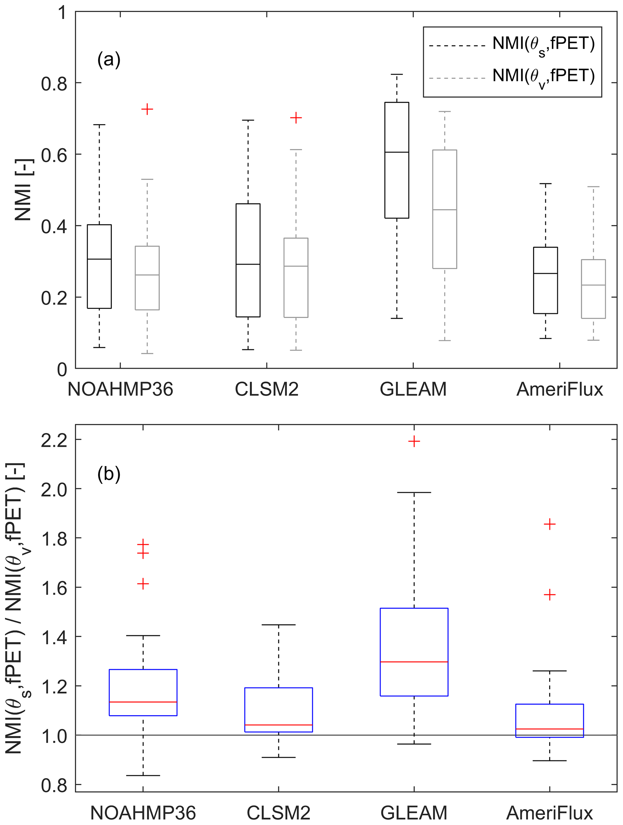
Figure 1 The θ ∕ ET coupling strengths for summertime anomaly time series acquired from various LSMs, GLEAM and AmeriFlux measurements: (a) NMI(θ_s, fPET) and NMI(θ_v, fPET) individually and (b) NMI(θ_s, fPET) normalized by NMI(θ_v, fPET).

In contrast, NMI(θ_s, fPET) and NMI(θ_v, fPET) values sampled from GLEAM θ and fPET estimates show positive biases (with median θ of about 0.5 and 0.4 [–] for NMI(θ_s, fPET) and NMI(θ_v, fPET), respectively) with respect to all other estimates.

Using the 34 AmeriFlux site-collocated samples pixels for a paired t test, both LSMs and GLEAM overall exhibit significantly (at the 0.05 level) higher NMI(θ_s, fPET) compared to NMI(θ_v, fPET), implying the surface soil water content observations contain more fPET information than vertically integrated soil water content observations. However, the observed difference between NMI(θ_s, fPET) and NMI(θ_v, fPET) is less discernible in AmeriFlux measurements (Fig. 1a).

Here, AmeriFlux observations are used as a baseline for LSM and GLEAM evaluation. However, it should be stressed that random observation errors in θ and fPET will introduce a low bias into AmeriFlux-based estimates of both NMI(θ_s, fPET) and NMI(θ_v, fPET; Crow et al., 2015) and thus their difference as well. To address this concern, Fig. 1b plots the ratio of NMI(θ_s, fPET) and NMI(θ_v, fPET), which effectively normalizes (and therefore minimizes) the impact of random observation errors. As discussed above, these ratio results illustrate the general tendency for NMI(θ_s, fPET) to exceed NMI(θ_v, fPET). They also highlight the tendency for GLEAM to overvalue θ_s (relative to θ_v) when estimating fPET. A second approach for reducing the random error of θ and fPET measurement errors is the correction based on triple collocation (TC) applied in Crow et al. (2015). However, this approach is currently restricted to linear correlations and cannot be applied to estimate NMI. Future work will examine extending the information-based TC approach of Nearing et al. (2017) to the examination of NMI.

3.2 Sensitivity of AmeriFlux-based NMI(θ_s, fPET) ∕ NMI(θ_V, fPET)

As mentioned in Sect. 2.1, an important concern is the impact of interpolation errors used to estimate 0–40 cm θ_v from AmeriFlux θ_s observations acquired at non-uniform depths. To ensure that different methods for calculating AmeriFlux θ_v values do not affect the main conclusion of this study, we configured three cases for θ_v calculation, and compared their NMI(θ_S, fPET) ∕ NMI(θ_v, fPET) results in Fig. 2. Case I reflects the baseline use of the exponential filter described in Sect. 2.1. However, slight changes to AmeriFlux results are noted if alternative approaches are used. Specifically, AmeriFlux-based NMI(θ_v, fPET) increases and closes the gap with NMI(θ_s, fPET) if the bottom-layer soil water content measurements are instead directly used as θ_v (Case II) or if 0–40 cm θ_v is based on the linear interpolation of the two AmeriFlux θ observations (Case III); the impact of this modest sensitivity on key results is discussed below.

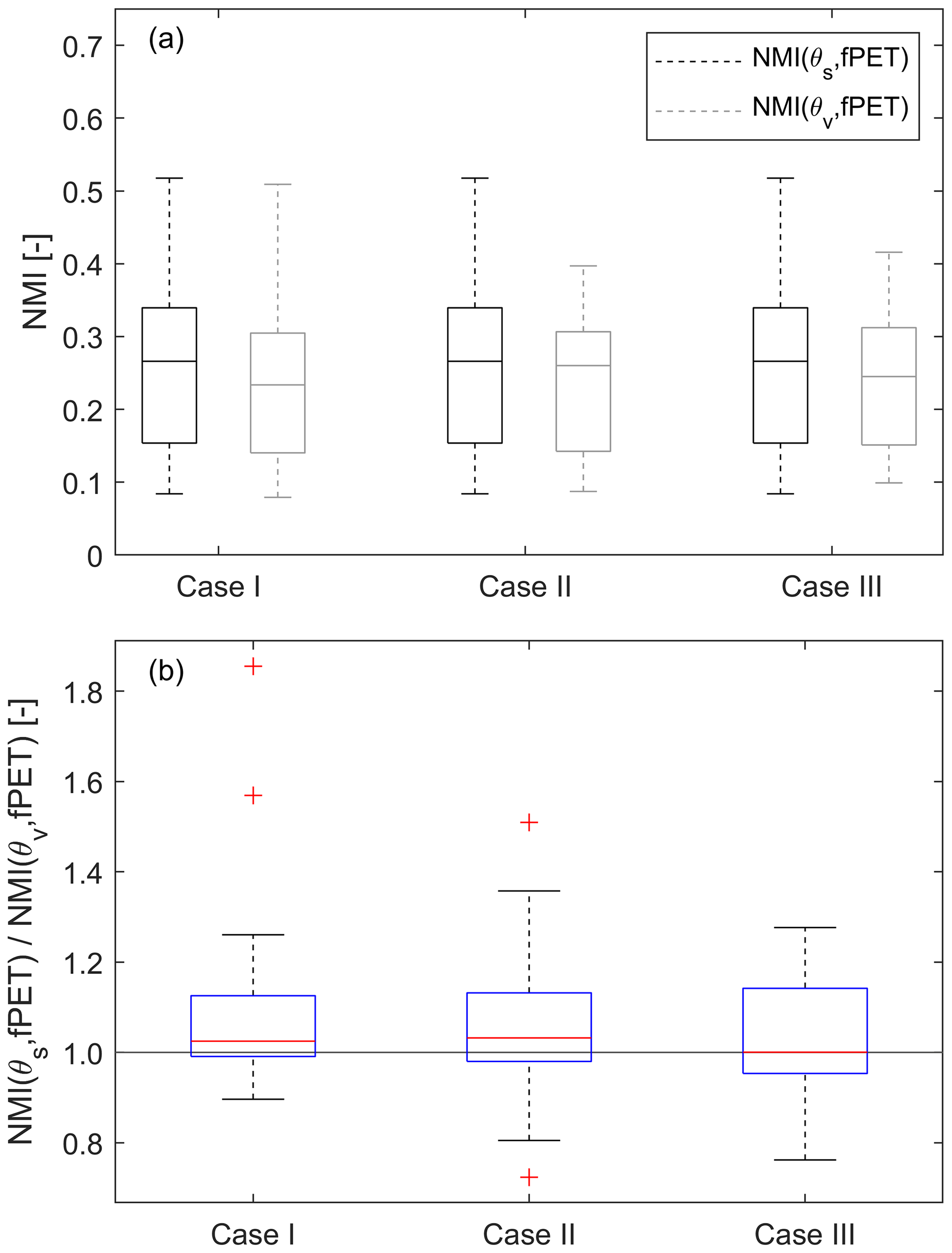
Figure 2 The θ ∕ ET coupling strengths for summertime anomaly time series from AmeriFlux measurements using three different θ_v calculation methods: (a) NMI(θ_s, fPET) and NMI(θ_v, fPET) individually and (b) NMI(θ_s, fPET) divided by NMI(θ_v, fPET) for multiple θ_v cases. Case I is based on the application of an exponential filter to extrapolate 0–10 cm θ_s to a consistent 0–40 cm bottom-layer depth, while Cases II and III refer to the direct use of only the bottom-layer measurement and a linear interpolation of both the top and bottom layer, respectively, to calculate θ_v (see Sect. 2.1 for details on each case).

In addition, switching from GLEAM- to NARR-based PET when calculating fPET for AmeriFlux-based NMI(θ_s, fPET) and NMI(θ_v, fPET) does not qualitatively change results and produces only a very slight (∼6 %) increase in the median NMI(θ_s, fPET) ∕ NMI(θ_v, fPET) ratio.

3.3 Spatial distribution of NMI(θ_s, fPET) and NMI(θ_v, fPET)

Figure 3 plots the spatial distribution of NMI(θ_s, fPET) and NMI(θ_v, fPET) results for each of the individual 34 AmeriFlux sites listed in Table 1. The climatic regime is represented by AI (aridity index) values plotted as the background color in Fig. 3. It can be seen in Fig. 3 that NMI(θ_s, fPET) estimates from LSMs and GLEAM are spatially related to hydro-climatic conditions, as NOAHMP and CLSM predict that θ_s is moderately coupled with fPET (i.e., NMI(θ_S, fPET) of 0.3–0.5 [–]) in the arid southwestern USA (AI < 0.2) and only loosely coupled with fPET in the relatively humid eastern USA. A similar decreasing trend of NMI(θ_s, fPET) from the southwestern to eastern USA is also captured by GLEAM. However, as noted above, GLEAM generally overestimates NMI(θ_s, fPET) and NMI(θ_v, fPET) compared to NOAHMP, CLSM and AmeriFlux. In contrast, a relatively weaker spatial pattern emerges in AmeriFlux-based NMI(θ_s, fPET) results. In addition, spatial patterns for NMI(θ_s, fPET) are less defined than for NMI(θ_v, fPET) in all four datasets.

Figure 3 NMI(θ_s, fPET) (left panels) and NMI(θ_v, fPET) (right panels) estimates at AmeriFlux sites for (a, e) NOAHMP, (b, f) CLSM, (c, g) GLEAM and (d, h) AmeriFlux. Marker color reflects NMI magnitudes and symbol type reflects local land-cover type at each site. Background color shading reflects aridity index (AI) values.

Scatterplots in Fig. 4 summarize the spatial relationship between LSM- and GLEAM-based NMI(θ_s, fPET) and NMI(θ_v, fPET) results versus AmeriFlux observations across different land use types. While observed levels of correlation in Fig. 4 are relatively modest, there is a significant level (p < 0.05) of spatial correspondence between modeled and observed NMI results only over forest sites, motivating the need to better understand processes responsible for spatial variations in NMI results. In addition, stratifying NMI(θ_s, fPET) ∕ NMI(θ_v, fPET) ratio results according to vegetation type (Fig. A1 in the Appendix) confirms that NMI(θ_s, fPET) slightly exceeds NMI(θ_v, fPET) across all vegetation types (and thus all rooting depths characterizing each vegetation type). This suggests that our analysis is not severely affected by variations in the depth of θ measurements. For further discussion on the impact of land cover on NMI results, please see Appendix A.

Figure 4 Scatterplot of LSM- and GLEAM-based (a, c, g, e) NMI(θ_s, fPET) and (b, d, f, h) NMI(θ_v, fPET) results versus AmeriFlux observations. Red symbols represent simulations from NOAHMP36; blue symbols represent simulations from CLSM2 and green symbols represent GLEAM retrievals.

3.4 Sensitivity of NMI(θ_s, fPET) ∕ NMI(θ_v, fPET) ratio to climatic conditions

Figure 5 further summarizes the NMI(θ_s, fPET) ∕ NMI(θ_V, fPET) ratio as a function of AI for all four products (NOAHMP, CLSM, GLEAM and AmeriFlux). Error bars represent the standard deviation of sampling errors calculated from a 500-member bootstrapping analysis. With increasing AI, there is a significant decreasing trend in both NMI(θ_S, fPET) and NMI(θ_v, fPET) for all three simulations, with a goodness of fit above 0.5 (figure not shown). For all cases, the NMI(θ_s, fPET) ∕ NMI(θ_v, fPET) ratios are consistently greater than unity under all climatic conditions. However, the estimated NMI(θ_s, fPET) ∕ NMI(θ_v, fPET) ratios from all three simulations (NOAHMP, CLSM and GLEAM) exhibit quite different trends with respect to AI. The NMI(θ_s, fPET) ∕ NMI(θ_V, fPET) ratio for CLSM decreases with increasing AI, with a moderate goodness-of-fit value of 0.28, while GLEAM estimates of NMI(θ_s, fPET) ∕ NMI(θ_v, fPET) shows an opposite increasing trend with increasing AI. Conversely, there is relatively lower sensitivity of the NMI(θ_s, fPET) ∕ NMI(θ_v, fPET) ratio to AI captured in the AmeriFlux measurements.

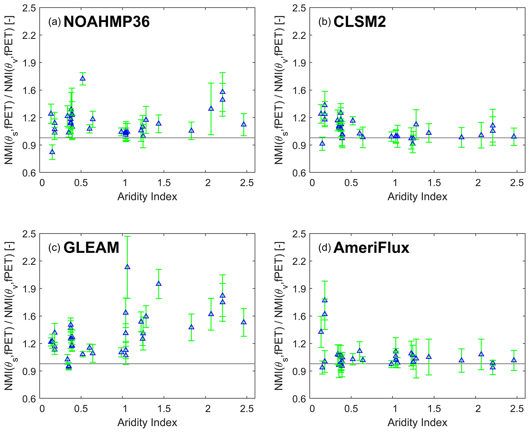
Figure 5 For (a) NOAHMP, (b) CLSM, (c) GLEAM and (d) AmeriFlux estimates, the ratio of NMI(θ_s, fPET) and NMI(θ_v, fPET) as a function of AI across all AmeriFlux sites.

Connecting these findings to the spatial distribution of NMI(θ_s, fPET) and NMI(θ_v, fPET; Fig. 3) confirms that the relative magnitudes of NMI(θ_s, fPET) and NMI(θ_v, fPET) for both LSMs and GLEAM are spatially related to hydro-climatic regimes. In contrast, this link is weaker in the AmeriFlux measurements which, except for a small fraction of very low AI sites, do not appear to vary as a function of AI. These conclusions are not qualitatively impacted by looking at NMI(θ_s, fPET) and NMI(θ_v, fPET) differences, as opposed to their ratio as in Fig. 5, or by looking at R(θ_s, fPET) and R(θ_v, fPET) instead of NMI.

4 Discussion and conclusion

Since transpiration dominates the global ET (Jasechko et al., 2013), deep-layer soil water content (θ_v) is generally considered to contain more ET information than that of surface soil water content (θ_s), given that plant transpiration is balanced by root water uptake from deeper soils (Seneviratne et al., 2010). However, this assumption is rarely tested using models and/or observations. Here, we apply normalized mutual information (NMI) to examine how the vertical support of a soil water content product affects its relationship with concurrent surface ET.

Specifically, using AmeriFlux ground observations, we examine whether (NMI-based) estimates of LSMs and GLEAM θ_s versus ET and θ_v versus ET coupling strength accurately reflect observations acquired at a range of AmeriFlux sites. In general, compared to the baseline case of exponential filter extrapolated 40 cm bottom-layer θ_v, LSMs and GLEAM agree with AmeriFlux observations in that the overall fPET information contained in θ_s is slightly higher than that of θ_v (Fig. 1). However, the sensitivity analysis showed this difference between NMI(θ_s, fPET) and NMI(θ_v, fPET) diminishes when using different methods for calculating θ_v using AmeriFlux observations (Fig. 2). As a result, this result should be viewed with caution.

While NOAHMP- and CLSM-derived NMI(θ_s, fPET) and NMI(θ_V, fPET) results are generally consistent with the AmeriFlux observations, GLEAM overestimates NMI(θ_s, fPET), NMI(θ_V, fPET) and the ratio NMI(θ_s, fPET) ∕ NMI(θ_V, fPET) relative to observations. Although both LSMs and GLEAM are based on the same classical two-section (soil water content-limited and energy-limited) ET regimes framework (Sect. 2.2), they differ in two fundamental aspects. First, the evaporative stress factor S is represented as a more direct and strong function of soil water content in GLEAM – see Eqs. (4) and (5) – which leads to the overestimation of the θ ∕ ET coupling strength. This is consistent with our results that GLEAM generally overestimates NMI(θ_s, fPET) and NMI(θ_v, fPET) consistently across all land covers, compared to AmeriFlux-based estimates. On the other hand, NOAHMP and CLSM approximate ET in the manner of biophysical models, and expresses biophysical control on ET through the stomatal resistance r_s, which is a function of multiple limiting factors including θ. Therefore, the more complex ET scheme employed by NOAHMP and CLSM would seem to mitigate the overestimation of NMI(θ_S, fPET) and NMI(θ_v, fPET), as other relevant factors besides θ (such as temperature, foliage nitrogen) are also considered in determining maximum carboxylation rate V_max and stomatal resistance r_s, and consequently more realistic actual ET.

Second, the stress factor β in both LSMs considers the cumulative effects of θconditions along different layers (Eq. 1), while the corresponding factor S in GLEAM only uses the wettest soil layer condition, which is top layer at most sites. This likely explains the overestimation of the NMI(θ_s, fPET) ∕ NMI(θ_v, fPET) ratio by GLEAM.

Nevertheless, we would like to stress that all approaches considered in our paper contain (at their core) a parameterized relationship between θ and ET. While the implications of mis-parameterizing this relationship are arguably more severe for a land surface model, we argue that the issue remains relevant for any approach (such as GLEAM) that utilizes a water balance (and/or data assimilation system) approach to estimate θ and, in turn, uses θ to constrain ET. Regardless of the complexity that a given approach employs, failing to accurately describe the relationship between ET and (large number of potential) environmental constraints should eventually degrade the robustness of the model, whether it is employed as a retrospective, diagnostic or predictive manner. To examine this issue directly, Fig. 6 plots the relationship between GLEAMS bias in NMI(θ_s, fPET) ∕ NMI(θ_v, fPET) ratio versus the RMSE of daily GLEAM ET simulations for a range of AmeriFlux sites. There is a positive correlation between the two quantities, which suggests that GLEAM overestimation of θ ∕ ET coupling during the summer may undermine the accuracy of its daily ET retrievals. It should be noted that GLEAM simultaneously overestimates both NMI(θ_s, fPET) and NMI(θ_v, fPET); however, the impact of this mis-parameterization impact on GLEAM ET accuracy is most obvious when plotted against the ratio NMI(θ_s, fPET) ∕ NMI(θ_v, fPET).

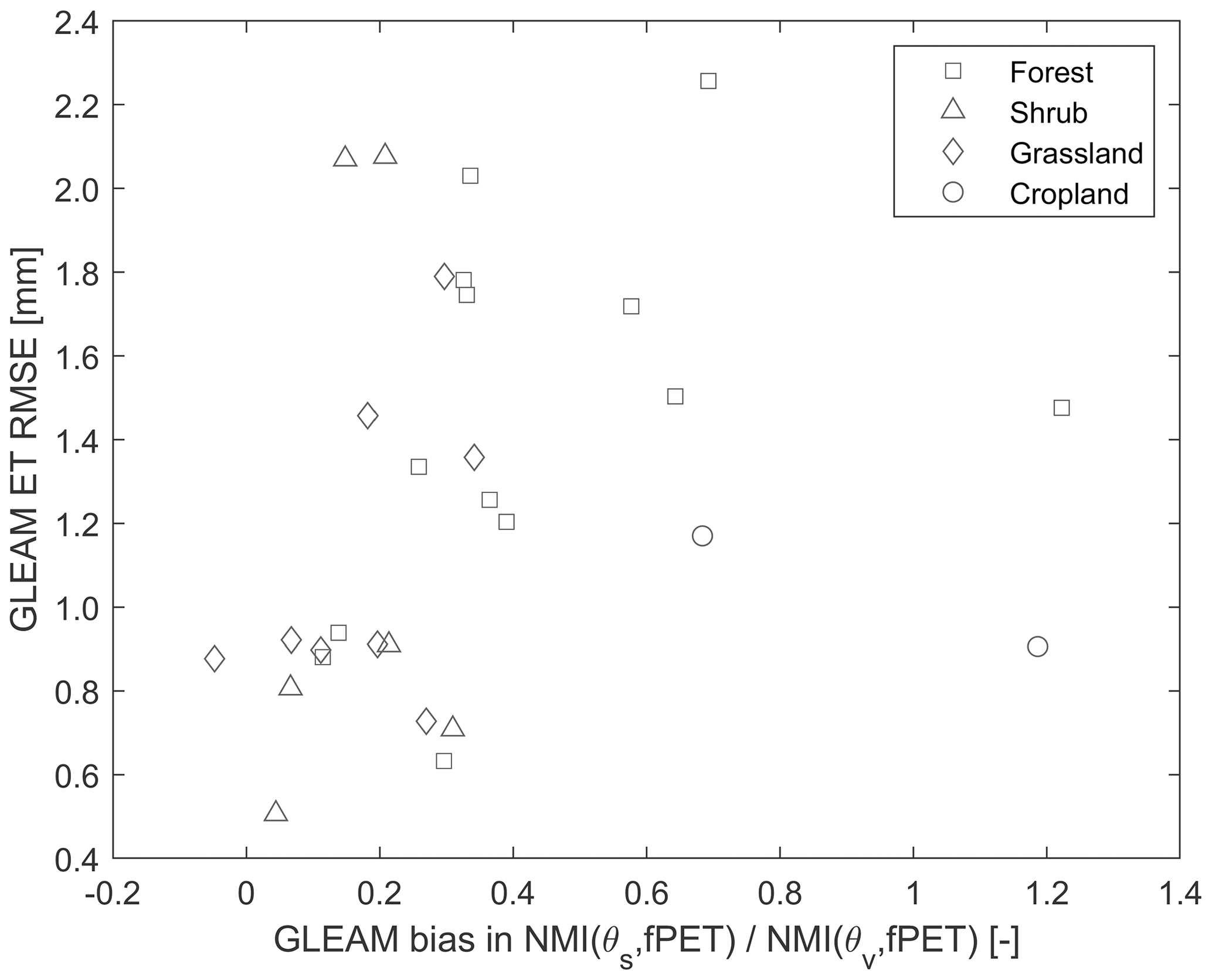
Figure 6 Daily ET error in GLEAM as a function of GLEAM bias in NMI(θ_S, fPET) ∕ NMI(θ_v, fPET) ratio across 34 AmeriFlux sites.

Although the median values of NMI(θ_s, fPET) and NMI(θ_V, fPET) predicted by NOAHMP and CLSM are generally in line with AmeriFlux observations, they are more spatially related to hydro-climatic conditions (as summarized by AI) than their counter parts acquired from AmeriFlux measurements. Seen from the plot of NMI(θ_s, fPET) ∕ NMI(θ_v, fPET) ratio as a function of AI (Fig. 5), the modeled and observed median of NMI(θ_s, fPET) ∕ NMI(θ_V, fPET) ratio decreases with increasing AI, and the decreasing trend is particularly clear when AI is lower than 1.0 [–]. In contrast, there is relatively lower sensitivity to aridity exhibited in the AmeriFlux measurements.

These results provide several key insights into future land–atmosphere coupling analysis and LSMs, as well as ET algorithm development. First, all the datasets – both model-based and ground-observed – indicate that θ_s contains at least as much ET information as θ_v. Hence, remote-sensing land surface soil water content datasets are suitable, and should be considered, for analyzing the general interaction between land and atmosphere, e.g., soil water content–air temperature coupling (Dong and Crow, 2019) and the interplay of soil water content and precipitation (Yin et al., 2014). Additionally, future generations of GLEAM may consider more sophisticated evaporation stress functions, which may improve its accuracy in representing the soil's control on local ET. This may, in turn, improve the accuracy of the GLEAM ET product. Finally, our results demonstrate that modeled θ ∕ ET is more sensitive to hydro-climates than the observed relationship. Modifying the model structures to reduce such sensitivity might be necessary for accurately representing the interaction of land surface and atmosphere across different climate zones. This may lead to more realistic projections of future drought-induced heat waves, when coupled with general circulation models.

Appendix A

We performed an additional sensitivity analysis to explicitly demonstrate the effect of different vegetation land-cover types and consequently different rooting depths (or θ_v measurement depths) on the NMI(θ_S, fPET) ∕ NMI(θ_v, fPET) ratio, and plotted these results in Fig. A1. The figure confirms that, consistent with AmeriFlux, both LSMs and GLEAM predict that NMI(θ_s, fPET) is slightly higher than NMI(θ_v, fPET) over most vegetation types, and GLEAM overestimates NMI(θ_s, fPET) ∕ NMI(θ_v, fPET) for most vegetation types.

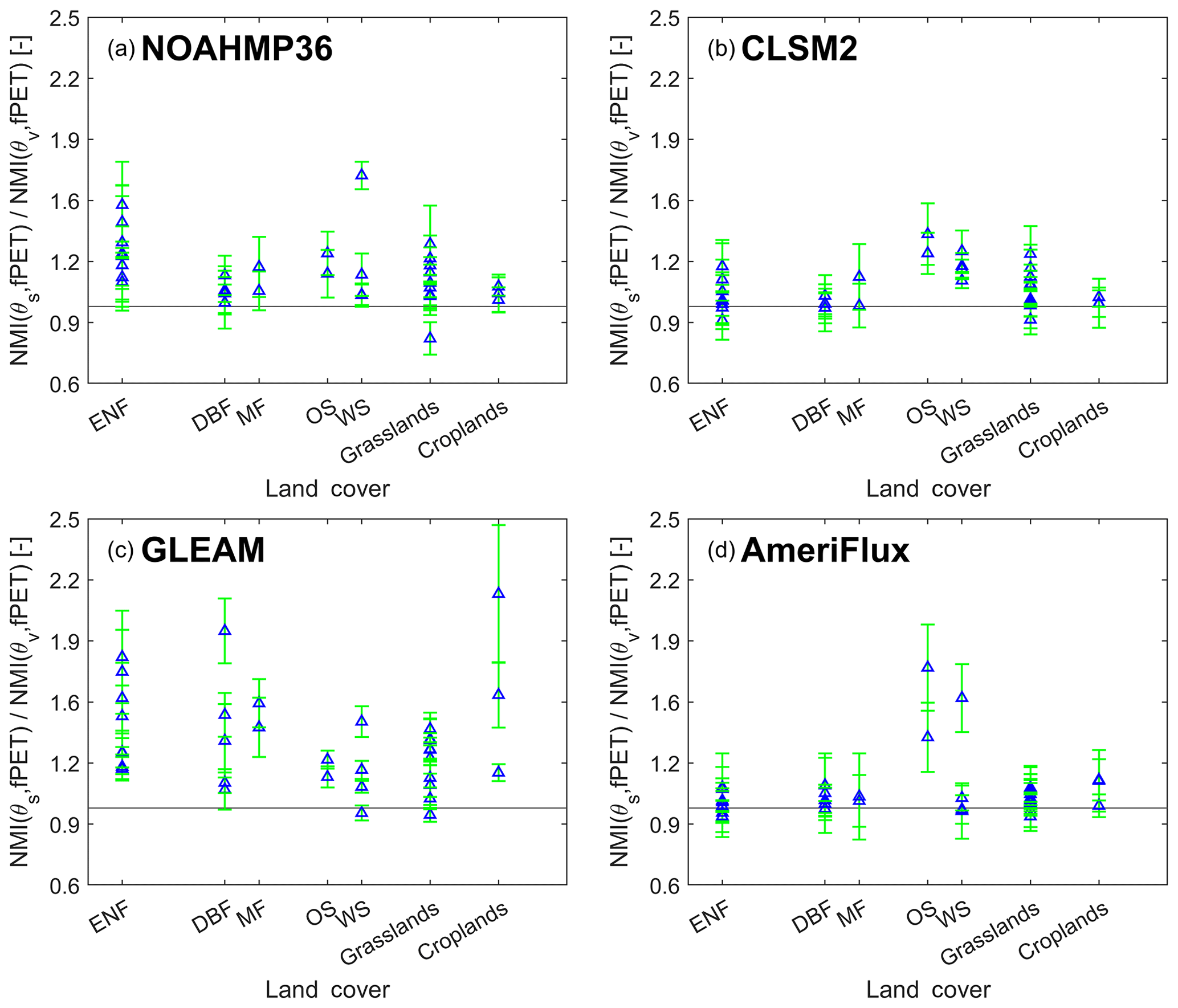
Figure A1 For (a) NOAHMP, (b) CLSM, (c) GLEAM and (d) AmeriFlux estimates, the ratio of NMI(θ_s, fPET) and NMI(θ_v, fPET) as a function of vegetation types across all AmeriFlux sites. “ENF”, “DBF”, “MF”, “OS” and “WS” represent evergreen needleleaf forests, deciduous broadleaf forests, mixed forests, open shrubland, and woody savannas, respectively.