A new form of the Saint-Venant equations for variable topography

The solution stability of river models using the one-dimensional (1D) Saint-Venant equations can be easily undermined when source terms in the discrete equations do not satisfy the Lipschitz smoothness condition for partial differential equations. Although instability issues have been previously noted, they are typically treated as model implementation issues rather than as underlying problems associated with the form of the governing equations. This study proposes a new reference slope form of the Saint-Venant equations to ensure smooth slope source terms and eliminate one source of potential numerical oscillations. It is shown that a simple algebraic transformation of channel geometry provides a smooth reference slope while preserving the correct cross-section flow area and the total Piezometric pressure gradient that drives the flow. The reference slope method ensures the slope source term in the governing equations is Lipschitz continuous while maintaining all the underlying complexity of the real-world geometry. The validity of the mathematical concept is demonstrated with the open-source Simulation Program for River Networks (SPRNT) model in a series of artificial test cases and a simulation of a small urban creek. Validation comparisons are made with analytical solutions and the Hydrologic Engineering Center's River Analysis System (HEC-RAS) model. The new method reduces numerical oscillations and instabilities without requiring ad hoc smoothing algorithms.

1 Introduction

The Saint-Venant equations (SVEs) for one-dimensional (1D) river modeling are typically presented with pressure forcing terms of either (i) gradients of the water surface elevation or (ii) thalweg bottom slope combined with gradients of the water depth. In this study, we demonstrate a new form using a reference slope (S_R) and its associated depth (h_a), which are shown to be algebraically identical to the two standard forms of the SVEs. The new forms provide greater flexibility in addressing numerical convergence issues associated with modeling discontinuous bottom slopes. A key point of this paper is that precise representation of the thalweg bottom slope (S₀) and hydrostatic pressure gradients ($\partial h_{\mathrm{0}}/\partial x$) is not necessary to correctly represent variable topography. Indeed, the splitting point for representing the forcing Piezometric pressure gradient as a body force (defined by a slope) and a residual head gradient term is free choice in a simple algebraic substitution. Different choices for the splitting provide different body force directions and lead to different forms of the SVEs – all of which are valid representations of variable topography and do not constitute a smoothing of topography. We will show that it is possible to use a smooth slope (body force) term in the SVEs without actually smoothing the topography. Herein, this smooth slope term will be designated as the reference slope, S_R, to distinguish it from the traditional thalweg bottom slope, S₀.

The two common differential forms of the SVEs are

$$\begin{array}{}\text{(1)}& {\displaystyle \frac{\partial Q}{\partial t}}+{\displaystyle \frac{\partial }{\partial x}}\left({\displaystyle \frac{Q^{\mathrm{2}}}{A}}\right)=-gA{S}_{\mathrm{f}}-gA{\displaystyle \frac{\partial \mathit{\eta }}{\partial x}}\end{array}$$

and

$$\begin{array}{}\text{(2)}& {\displaystyle \frac{\partial Q}{\partial t}}+{\displaystyle \frac{\partial }{\partial x}}\left({\displaystyle \frac{Q^{\mathrm{2}}}{A}}\right)=-gA{S}_{\mathrm{f}}+gA{S}_{\mathrm{0}}-gA{\displaystyle \frac{\partial h_{\mathrm{0}}}{\partial x}},\end{array}$$

where Q is the flow rate, A is the cross-section area, η is the water surface elevation, h₀ is the thalweg depth, S₀ is the thalweg bottom slope, and S_f is the friction slope that represents the local energy gradient. Equation (1) can be envisioned as using the Piezometric head gradient to force the flow, as shown in Fig. 1a. In contrast, Eq. (2) can be envisioned as splitting the Piezometric gradient into a body force in the bottom slope direction and a hydrostatic head gradient, as shown in Fig. 1b. Note that both equations are valid for variable topography despite only the second equation explicitly representing the bottom slope and thalweg depth hydrostatic pressure gradients.

Figure 1 The η form of the SVEs (a) has a driving Piezometric head gradient which is equivalent (b) to the sum of the hydrostatic head gradient and a body force aligned with S₀. The effect of varying geometry is handled in A in both forms.

The two SVE forms of Eqs. (1) and (2) are algebraically identical using the identity

$$\begin{array}{}\text{(3)}& {\displaystyle \frac{\partial \mathit{\eta }}{\partial x}}\equiv {\displaystyle \frac{\partial h_{\mathrm{0}}}{\partial x}}-S_{\mathrm{0}}.\end{array}$$

Heuristically, we can propose a more general identity of

$$\begin{array}{}\text{(4)}& {\displaystyle \frac{\partial \mathit{\eta }}{\partial x}}\equiv {\displaystyle \frac{\partial h_{\mathrm{a}}}{\partial x}}-S_{\mathrm{R}},\end{array}$$

where S_R is an arbitrary reference slope and h_a is an associated depth that will be defined in Sect. 3.2 below. For an introductory exposition, $\partial h_{\mathrm{a}}/\partial x$ is merely the residual implied for a given $\partial \mathit{\eta }/\partial x$ and arbitrary S_R. Applying Eq. (4) to (1) provides the following:

$$\begin{array}{}\text{(5)}& {\displaystyle \frac{\partial Q}{\partial t}}+{\displaystyle \frac{\partial }{\partial x}}\left({\displaystyle \frac{Q^{\mathrm{2}}}{A}}\right)=-gA{S}_{\mathrm{f}}+gA{S}_{\mathrm{R}}-gA{\displaystyle \frac{\partial h_{\mathrm{a}}}{\partial x}},\end{array}$$

where the terms gAS_R and $gA\frac{\partial h_{\mathrm{a}}}{\partial x}$ are algebraically equivalent to those in Eqs. (1) and (2). Clearly, if we let S_R equal S₀, then h_a equals h₀ and we recover Eq. (2). Furthermore, if we let S_R equal 0, then h_a equals η and we recover Eq. (1). The equations are identical with these substitutions, so it follows that using a reference slope of zero (S_R=0) must exactly represent the same topographic variability as using a reference slope that mimics the topographic slope (S_R=S₀) as long as h_a is correctly defined consistent with Eq. (4). That is to say that from simple algebra the use of the real S₀ in the SVEs is not required to capture effects of topographic variability as long as the depth gradient term is correctly redefined as something other than the thalweg depth gradient and the cross-section flow areas are correctly computed.

From the arguments above, the effects of varying bottom topography are captured by S_R=0 and h_a=η, which implies we are also free to introduce any other (preferably smooth) S_R into Eq. (5) without altering the underlying representation of variable topography. An example is illustrated in Fig. 2. As the splitting defined in Eq. (4) makes Eq. (5) algebraically identical to Eqs. (1) and (2), the introduction of a smooth S_R does not reflect “smoothing” of the topography. It merely reflects a decision on whether effects of non-smoothness will reside solely in solution variables A and h_a or will also be forced as a non-smooth source term in S₀.

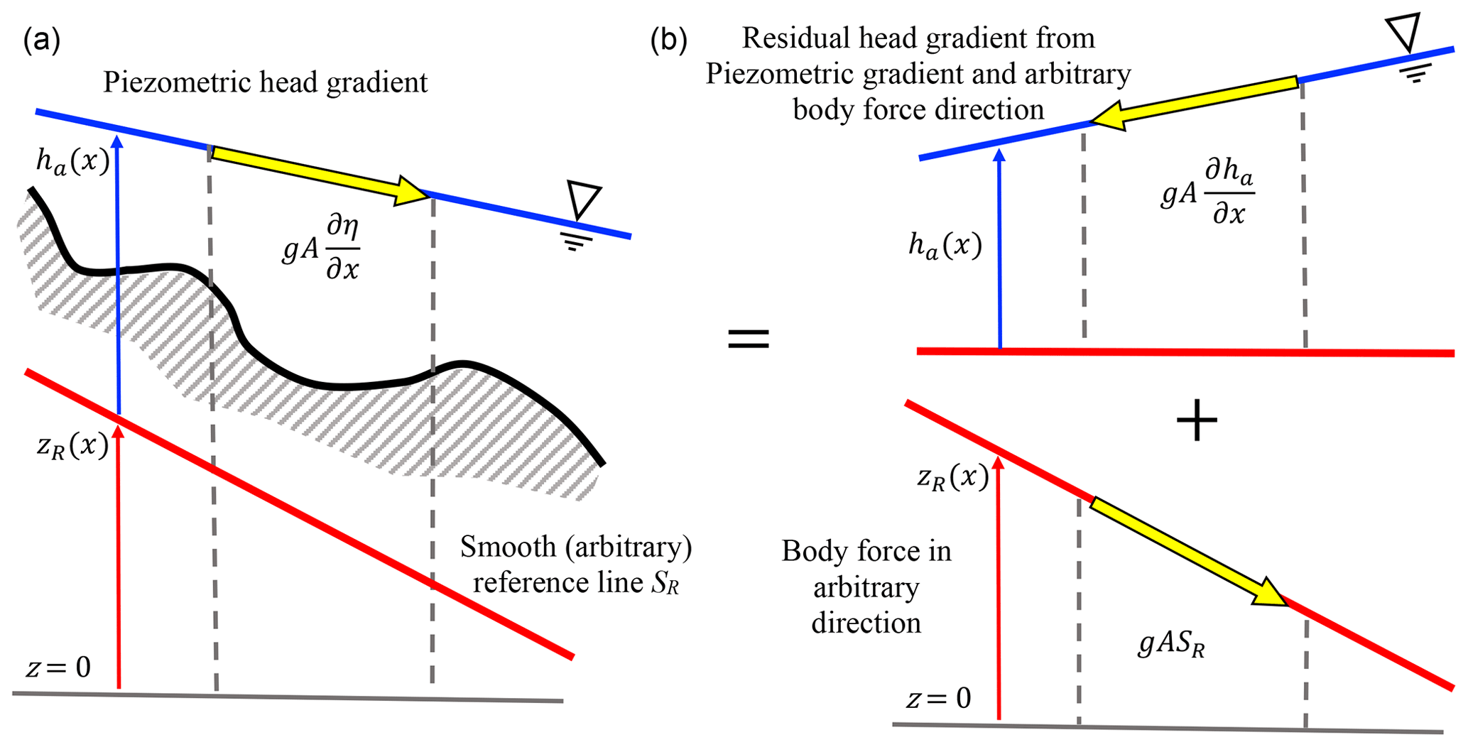
Figure 2 Comparison of Piezometric forcing terms for varying topography. (a) Eq. (1) with the arbitrary S_R line provided for reference. (b) The equivalent split form of forcing with Eq. (5) using the identity of Eq. (4). The physical bottom topography, shown only in (a) for clarity, only plays a role through the cross-section area (A) which feeds back into the solution of variability in h_a in both forms of the equation.

We would like to use an a priori smooth S_R in a computational model rather than the actual thalweg S₀ because of what happens to S₀(x) and $\partial h_{\mathrm{0}}\left(x\right)/\partial x$ for topography varying sharply over short distances, as illustrated in Fig. 3. From a physics perspective, using S₀ to split the Piezometric head is an intuitive way to describe the local interplay of pressure with the bottom slope. Furthermore, S₀ has the advantage of being readily reduced to a kinematic wave equation where S_f=S₀, which has some advantage in multipurpose codes. However, from a numerical modeling perspective, using S₀ has a significant limitation based on its smoothness. If the water surface is smooth, then non-smooth S₀(x) requires the numerical solver to produce a compensating non-smooth h₀(x), i.e., requiring a well-balanced scheme (see Sect. 2). If we can discard our (wrong) intuition that the S₀ form must somehow better represent sharply variable topography – i.e., recognizing the algebraic equivalence of Eq. (5) with Eqs. (1) and (2) – it follows that the splitting of the Piezometric head to include a body force that is everywhere exactly aligned with a sharply varying S₀ is (from a numerical perspective) merely creating unnecessary complexity in the governing equation source term that requires compensating complexity in the solution algorithm. In contrast, by requiring S_R to be smooth, we can ensure the h_a solution is also smooth for a smoothly varying free surface.

Figure 3 Comparison of Piezometric forcing terms with sharply varying topography for Eqs. (1) and (2). (a) The Piezometric head gradient for Eq. (1). (b) The equivalent split form of forcing from Eq. (2) using the identity of Eq. (3). The variability of the bottom of (a) will be reflected in the cross-section area, A(x), that feeds back into the solution of η(x). In contrast, (b) attempts to directly represent topographic variability as both a driving term in S₀(x) and a solution response term, h₀(x)

The use of S_R rather than S₀ in the governing equations can perhaps be better understood if we think of the slope in Eq. (4) as representing simply a portion of the overall Piezometric pressure gradient that can be extracted from $\partial \mathit{\eta }/\partial x$ and treated as a body force that varies gradually along the channel. Hence, in Fig. 3 we are not interested in separating out the details of the sharply varying slope changes in the local topography but instead prefer a body force term that aligns with the mean slope over some larger spatial scale, e.g., as in Fig. 2.

In this paper, we examine the effect of variable cross-section geometry on numerical solutions of the SVEs and propose a new reference slope approach that can be inferred from the above arguments. The use of a reference slope as a body force direction to split the Piezometric head gradient term ensures (i) the slope used in the discrete source term is smooth, (ii) the variable geometry is correctly retained, (iii) the fundamental governing equations are preserved, and (iv) an SVE numerical algorithm developed using S₀ is essentially unchanged. We further demonstrate that bottom slope discontinuities are a cause of problems in finite-difference forms of 1D Saint-Venant equations with subcritical flow. Of course, this idea will not be a surprise to many modelers who routinely remove troublesome cross sections or smooth their topography; however, the concept does not appear to have been conclusively demonstrated in the literature. More importantly, we show that the problem is inherent in the traditional formulation of the governing equations using the thalweg bottom slope, S₀, which is usually computed as the slope between the lowest points in two adjacent river cross sections. Problems associated with slope discontinuities can be fixed within the governing equations by the careful selection of smoothly changing reference elevations along the channel, z_R(x), which results in smooth reference slopes, S_R(x), and the redefinition of the thalweg depth (h₀) as a depth associated (h_a) with the reference elevation. Note that h_a is not necessarily any characteristic depth of the flow and is only indirectly related to the hydrostatic pressure.

The approach proposed herein can be implemented within any Saint-Venant model as it is entirely independent of the solution algorithm; however, implementation does require rewriting code for the relationships between cross-section area, wetted perimeter, and the depth variable of the solution. Note that the new approach includes a redefinition of the depth variable (traditionally the maximum depth, h₀) as the depth associated (h_a) with the reference elevation, z_R.

2 Background

One-dimensional (1D) hydrodynamic models using the Saint-Venant equations (SVEs) are widely employed for studying both natural streams and man-made channels (e.g., Martinez-Aranda et al., 2019; Sanders, 2001). It is widely recognized that numerical solutions of the SVEs are prone to spurious oscillations in the free-surface elevation unless particular care is taken in the numerical formulation and/or the problem definition (e.g., Nujic, 1995; Tseng, 2004). Numerous techniques and special numerical schemes have been previously designed to overcome unwanted numerical oscillations caused by discontinuous geometries and boundary conditions (e.g., Zhou et al., 2001; Liang and Marche, 2009). These approaches typically rely on the concept of a well-balanced discrete form (Greenberg and LeRoux, 1996) as discussed in a comprehensive review by Kesserwani (2013) and further elaborated by Hodges (2019).

Although well-balanced schemes are relatively robust in handling discontinuous boundary conditions, they have not been extensively applied in water resource models to simulate the regional-to-continental-scale river networks or stormwater systems for megacities. The rapidly varying and discontinuous S₀ in natural systems can significantly increase the difficulty and computational burden of obtaining a well-balanced method (Schippa and Pavan, 2008). Hence, when a large-scale open-channel model develops oscillations and/or instabilities, practitioners may resort to the traditional approach of removing cross sections or smoothing bathymetry to mitigate oscillatory or unstable solution behavior (Tayfur et al., 1993). Such ad hoc efforts can be effective as they address a major cause of such oscillations and instabilities (discontinuous topography), but they inherently reduce the fidelity of the simulation.

Oscillations and instabilities can be induced in any numerical solution of a boundary initial value problem by the inclusion of non-smooth source terms; i.e., if we consider an advection equation of the form

$$\begin{array}{}\text{(6)}& {\displaystyle \frac{\partial Q}{\partial t}}+{\displaystyle \frac{\partial }{\partial x}}\left({\displaystyle \frac{Q^{\mathrm{2}}}{A}}\right)=\mathit{\sigma },\end{array}$$

where σ is a nonhomogeneous source term, a fundamental theorem for differential equations provides that a unique solution cannot be guaranteed to exist unless the source term is Lipschitz continuous (e.g., Iserles, 1996). That numerical instabilities are often caused by non-smooth source terms is not a new observation. A wide variety of numerical schemes have been developed to address this issue, including, e.g., extensive work on wetting/drying (Liang and Marche, 2009; Song et al., 2011), positivity-preserving methods for coupled models (Singh et al., 2015), and implicit schemes that address stiffness of the nonlinear friction term (Xia and Liang, 2018). The literature in this area is vast – particularly if both 1D and 2D models are considered. For the present purposes, we focus on only one part of the source term, S₀, whose non-smoothness has previously been treated as a problem to be handled rather than as a problem that can be directly eliminated in the governing equations. Existing well-balanced schemes (see reviews noted above) seek to compensate for non-smoothness of all parts of the source term in the structure of the numerical discretization. Arguably, if the slope term is guaranteed smooth, then a well-balanced scheme should be simpler to create. In general, when the thalweg bottom slope (S₀) appears as a source term in the SVEs, it should be a priori Lipschitz smooth or oscillations and instabilities should be expected. For natural systems, S₀(x) is typically defined using the maximum channel depth at each surveyed cross section, which is rarely a smooth function (unless the distance between cross sections is large compared to bottom elevation variability). When cross sections are surveyed at short distances, S₀ will tend to have significant variability. It follows that the use of S₀ has the undesirable property that smaller Δx (i.e., resolving a river with more detailed survey data) will increase the non-smoothness in this source term of the momentum equation, resulting in a model that is unlikely to converge under a grid refinement test. It is not surprising that S₀ smoothness, when it occurs in a model of a natural river channel, is typically the result of relatively long separations (Δx) between cross-section surveys that ensures that the discrete d²z₀∕dx² is small. Thus, removing cross sections can be an effective mitigation technique because it increases Δx and effectively smooths S₀. In general, models discretized with higher-resolution river surveys (smaller Δx) will have greater non-smoothness in S₀ and develop more oscillation and instability issues. In essence, our models get worse as our boundary condition data get better.

The problems associated with S₀ can be understood by considering the identity in Eq. (3) for a channel with subcritical flow in which the free-surface curvature is expected to be negligible, i.e., ${\partial }^{\mathrm{2}}\mathit{\eta }/\partial x^{\mathrm{2}}\sim \mathit{ϵ}$, where $\mathit{ϵ}\ll \text{d}{S}_{\mathrm{0}}/\text{d}x,{\partial }^{\mathrm{2}}\mathit{\eta }/{\partial }^{\mathrm{2}}x$. Taking the along-channel gradient of Eq. (3) implies that

$$\begin{array}{}\text{(7)}& {\displaystyle \frac{{\partial }^{\mathrm{2}}{h}_{\mathrm{0}}}{\partial x^{\mathrm{2}}}}={\displaystyle \frac{\text{d}{S}_{\mathrm{0}}}{\text{d}x}}-\mathit{ϵ}.\end{array}$$

Thus, forcing with a non-smooth dS₀(x)∕dx will require non-negligible curvature of the response variable, h₀(x), whose gradient is also a forcing function of the nonlinear equation. Feedback can easily build and cause successive overshoot/undershoot effects, producing oscillations and non-convergence in a nonlinear solver. In contrast, Eq. (4) can be invoked with dS_R∕dx guaranteed to be small, which implies that ${\partial }^{\mathrm{2}}{h}_{\mathrm{a}}/\partial x^{\mathrm{2}}$ will also be small even when $\partial A/\partial x$ is non-smooth. As a practical matter, any S₀ with a discontinuous discrete first derivative (i.e., discontinuities in the second derivative of the thalweg elevation, d²z₀∕dx²) will be Lipschitz discontinuous and should not be directly discretized in an SVE solution with Eq. (2). Although approximate numerical solutions of equations with non-smooth S₀(x) can sometimes be attained for models with sufficient damping, such solutions are questionable as they do not have rigorous mathematical foundations.

Arguably, non-smoothness in S₀ can be handled in one of four ways: (i) smoothing the geometry – hence solving for flows that do not match the real system; (ii) applying ad hoc smoothing within the flow solution – i.e., adjusting the physics to remove numerical instabilities; (iii) adjusting the numerical discretization scheme to compensate for non-smoothness – e.g., the well-balanced concept; or (iv) adjusting the governing equations to ensure that any slope in the source term is smooth without modifying the solution physics, the channel geometry, or the numerical discretization scheme. It should be obvious that Eq. (1) is the extreme example of the last approach – replacing S₀ and $\partial h_{\mathrm{0}}/\partial x$ with $\partial \mathit{\eta }/\partial x$ ensures that S₀ does not occur in the governing equations and cannot destabilize the solution. To our knowledge, the last approach (as used herein and illustrated in Fig. 2) has not been previously proposed or analyzed in the literature. Nevertheless, as shown below, it provides a simple method that can be readily adapted into existing hydrodynamic models.

For brevity, we will limit our focus herein to subcritical flows – backwater tends to smooth the effects of slope discontinuities and thus we expect smooth solutions for flow rate and free-surface elevation despite non-smooth geometry. Nevertheless, common SVE solvers can exhibit oscillatory, non-convergent behavior even in simple subcritical flows when geometry is not smooth. In the following, it will be obvious that the mathematical theory applies directly to supercritical and transcritical flows as well, but evaluating model performance under the breadth of possible transcritical conditions (including non-smooth jumps) necessarily requires more analyses than is practical in a single paper.

3 Methods

3.1 SPRNT

The Simulation Program for River Networks (SPRNT) code for unsteady SVE river networks is used and modified herein. The baseline for this code models momentum using Eq. (2), which is coupled to the solution of continuity,

$$\begin{array}{}\text{(8)}& {\displaystyle \frac{\partial A}{\partial t}}+{\displaystyle \frac{\partial Q}{\partial x}}=q_{\mathrm{\ell }},\end{array}$$

where q_ℓ is a lateral inflow per unit length. Note that significantly non-smooth q_ℓ(x,t) can provide another source of numerical oscillations and instability (Kuiry et al., 2010). As the main focus of this study is the slope source term in the momentum equation, the lateral inflows and their effects are neglected by setting q_ℓ=0 everywhere.

In the SPRNT momentum equation, the friction slope is represented using the Chezy–Manning form as

$$\begin{array}{}\text{(9)}& S_{\mathrm{f}}={\displaystyle \frac{n^{\mathrm{2}}{P}_{\mathrm{w}}^{\mathrm{4}/\mathrm{3}}}{A^{\mathrm{10}/\mathrm{3}}}}{Q}^{\mathrm{2}},\end{array}$$

where P_w is the wetted perimeter of a cross section and n is the Gauckler–Manning–Strickler roughness. Although, there are other methods for treating frictional losses (e.g., Decoene et al., 2009; Burguete et al., 2007), the Chezy–Manning form remains popular due to its simplicity.

The baseline model uses the thalweg elevation (z₀), the thalweg depth (h₀), and the thalweg bottom slope (S₀) as

$$\begin{array}{}\text{(10)}& h_{\mathrm{0}}\equiv \mathit{\eta }-z_{\mathrm{0}}\end{array}$$

and

$$\begin{array}{}\text{(11)}& S_{\mathrm{0}}\equiv -{\displaystyle \frac{\partial z_{\mathrm{0}}}{\partial x}}.\end{array}$$

SPRNT is an open-source, 1D hydrodynamic solver using the fully implicit Preissmann numerical scheme (Preissmann, 1961) with the Newton–Raphson iteration and computational acceleration techniques developed from very large-scale integration (VLSI) semiconductor design. Details on the baseline SPRNT model and its application to large river networks are provided in Liu and Hodges (2014) and Yu et al. (2017).

3.2 Reference slope method

We introduce a new reference slope (RS) method through a transformation and redefinition of geometry in the Saint-Venant equations, as discussed in Sect. 1. In place of the conventional h₀ and z₀, we define a reference elevation (z_R) and its associated depth (h_a) as shown in Fig. 4. These provide a relationship with the free-surface elevation (η) defined as

$$\begin{array}{}\text{(12)}& h_{\mathrm{a}}\equiv \mathit{\eta }-z_{\mathrm{R}}.\end{array}$$

Note that z_R is arbitrary, so h_a may be either greater than or less than the thalweg depth, h₀, at a given location. As shown in Fig. 4, it is convenient to define the reference height, h_R, in relation to z_R and the true bottom elevation, z₀, by

$$\begin{array}{}\text{(13)}& h_{\mathrm{R}}\equiv z_{\mathrm{0}}-z_{\mathrm{R}}.\end{array}$$

Thus, the conventional h₀ and z₀ are recovered with

$$\begin{array}{}\text{(14)}& h_{\mathrm{0}}=h_{\mathrm{a}}-h_{\mathrm{R}}\end{array}$$

and

$$\begin{array}{}\text{(15)}& z_{\mathrm{0}}=z_{\mathrm{R}}+h_{\mathrm{R}}.\end{array}$$

We define the reference slope (S_R) as the downstream slope of z_R:

$$\begin{array}{}\text{(16)}& S_{\mathrm{R}}\equiv -{\displaystyle \frac{\partial z_{\mathrm{R}}}{\partial x}}.\end{array}$$

Using Eqs. (12) and (16) in Eq. (2) provides Eq. (5), which is more conveniently written as

$$\begin{array}{}\text{(17)}& {\displaystyle \frac{\partial Q}{\partial t}}+{\displaystyle \frac{\partial }{\partial x}}\left({\displaystyle \frac{Q^{\mathrm{2}}}{A}}\right)=-gA{\displaystyle \frac{\partial h_{\mathrm{a}}}{\partial x}}+gA\left(S_{\mathrm{R}}-S_{\mathrm{f}}\right).\end{array}$$

The above is identical to Eq. (2) with the simple substitution of h_a and S_R for h₀ and S₀. In this formulation, the definition of z_R(x) is arbitrary, so we can a priori require a definition such that S_R(x) is smooth. A trivial choice that is guaranteed smooth is z_R(x)=constant, which returns S_R(x)=0 and the Saint-Venant equations in the form of Eq. (1). However, this form with $\partial \mathit{\eta }/\partial x$ for the entire pressure term is known to cause numerical stiffness issues for large ranges in η, e.g., the elevation change in a river from its mountain source to a coastal plain (Liu and Hodges, 2014). Using the conventional S₀ in Eq. (2) reduces this problem as the range of h₀ is inherently confined to the local water depths rather than the underlying topography. In the RS method, the range of h_a is tied to the range of water depths and the selection of z_R; thus, for present purposes, we are interested in nontrivial definitions of z_R that (i) are close to z₀ to maintain a small range of h_a values and (ii) provide smooth S_R(x). An arbitrary z_R that is far from z₀ or non-smooth is of little interest as it holds no theoretical or practical advantage over the Eq. (1) approach implied by S_R(x)=0.

If S_R(x) is required to be smooth, then the source term of the equation can be guaranteed smooth as long as S_f(x) is smooth, which is typically true as long as the solution, Q(x), is smooth. Note that in extreme cases of geometric discontinuity the combined values of n, P_w, and A in Eq. (9) can cause a non-Lipschitz friction term; thus, the RS method cannot guarantee that the entire source term is smooth. Numerical solution methods are usually robust against discontinuities in n and P_w as they are coefficients of the solution variables {A,Q}. More subtle problems might arise due to discontinuities developed in the $Q^{\mathrm{2}}{A}^{-\mathrm{10}/\mathrm{3}}$ ratio in Eq. (9); countering incipient instabilities from this term requires other numerical strategies (e.g., Xia and Liang, 2018).

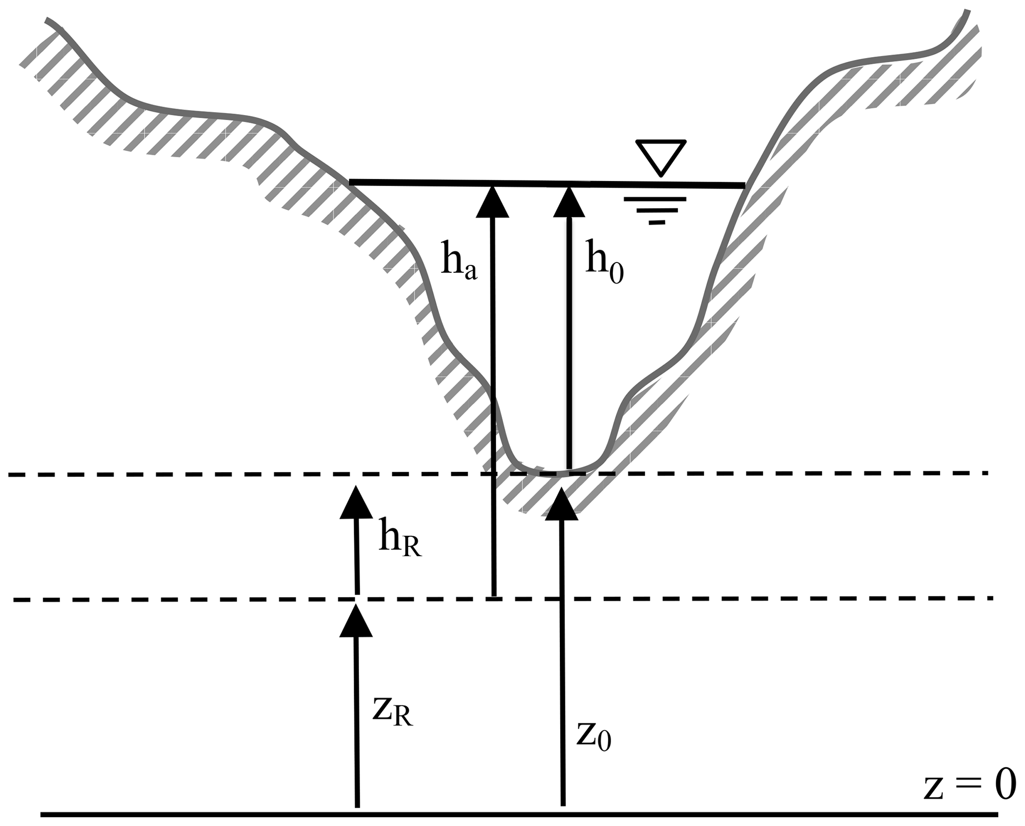
Figure 4 Relationships of h_a, h_R, z_R, and z₀ for an arbitrary cross section. Note that z_R>z₀ is also allowed, which results in h_a<h₀ and a negative value for h_R. Furthermore, if z_R is greater than z₀+h₀, then h_a is negative to retain algebraic consistency. Modified from Liu (2014) and used with permission.

A critical change required by the introduction of h_a is that the conventional geometric auxiliary relationships of A=f(h₀) and P_w=f(h₀) must be transformed into A=f(h_a) and P_w=f(h_a). That is, once we change the depth in our equation from h₀ to h_a, we must re-index the geometry. In general, for known functions A(h₀) and P_w(h₀) this is a trivial transformation:

$$\begin{array}{}\text{(18)}& A=A(h_{\mathrm{a}}-h_{\mathrm{R}})\end{array}$$

and

$$\begin{array}{}\text{(19)}& P_{\mathrm{w}}=P_{\mathrm{w}}(h_{\mathrm{a}}-h_{\mathrm{R}}).\end{array}$$

However, the implementation in an existing code is not necessarily as simple as the above equations suggest. For example, in Fig. 4, the condition A=0 occurs when h_a=h_R, i.e., a nonzero value as compared to h₀=0 with conventional geometry. Unfortunately, model developers typically have ad hoc wetting/drying treatments that are introduced as h₀→0 or for h₀<0. Such treatments need to be modified to be deployed as h_a→h_R, which introduces the added complication that h_R is negative when z_R>z₀. Note that the new geometry does not require altering the wetting/drying algorithm itself or, for that matter, any other solution algorithm – only the actual geometry definitions require alteration. These relatively straightforward changes can be contrasted with the effort needed to provide a well-balanced numerical discretization scheme for the conventional S₀ representation of geometry (e.g., Kesserwani, 2013).

The modification of the SPRNT code to implement the above RS method will be known as SPRNT-RS. The SPRNT and SPRNT-RS source codes are available in an open-source repository (Liu, 2014). Note that the solution algorithm for SPRNT-RS is identical to that of SPRNT; the only code changes are for the new geometry definitions for h_a and S_R that replace h₀ and S₀ in the original algorithm. This simple geometry replacement strategy is effective because Eq. (17) is identical to Eq. (2) except for the change in nomenclature to h_a and S_R.

3.3 Generating a smooth S_R(x)

The z_R(x) and hence S_R(x) are arbitrary choices in the RS method but should be generated for the smoothness of S_R(x) along the reach. In synthetic reach test cases and analytical test cases (described below), the channels are a priori either specified with a uniform S_R or produced by a different order of splines. For our urban creek test case, the z_R is generated with an approximating cubic B-spline (de Boor, 2001) based on thalweg, z₀(x), elevations. There are a variety of possible ways to generate smooth S_R(x), but applying approximating cubic B-splines to the z₀(x) is convenient because the slope is guaranteed to be locally smooth as long as the knot spacing in the B-spline is everywhere larger than the spacing between cross sections. It should be emphasized that an exact spline fitting of all the thalweg data (i.e., knots at all the cross sections) will be smooth at scales finer than the cross-section spacing but non-smooth at the model's discretization scale. That is to say that the exact cubic spline fitting of z₀(x) does not reduce discontinuities at the discretization scale – only an approximate fitting associated with coarser scales than the cross-section spacing will be effective. It follows that there is some (limited) choice in the selection of the subset of z₀(x) used as the spline knots, with different sets producing slightly different {z_R(x),h_R(x)} over the domain. Each set is algebraically identical to the underling geometry, so the generated solutions should be identical within the machine truncation error as long as the z_R(x) are sufficiently smooth. Implications of the method chosen for generating z_R(x) are discussed in Sect. 5.3. Further details and test cases are provided in Yu et al. (2019b).

3.4 HEC-RAS for model validation

The baseline SPRNT has been previously shown to have excellent agreement with the Hydrologic Engineering Center's River Analysis System (version 5.0.7) – known as HEC-RAS. Liu and Hodges (2014) showed SPRNT simulations agreed with HEC-RAS with ≤3 % difference in water depth solution when using both prismatic cross sections and nonuniform channels. Thus, HEC-RAS provides a reasonable model for testing and validating SPRINT-RS. We would have preferred to use a single model with and without the RS method for such model–model comparisons; however, HEC-RAS is a closed-source proprietary model, so we could not directly implement and test the RS method in that code. Conversely, as expected by the discussions in Sect. 2, the baseline SPRNT model is oscillatory and non-convergent on the highly discontinuous geometry of our test cases due to its use of the S₀ approach, so it cannot be directly used for before and after comparisons of RS. Thus, simulations using SPRNT-RS are compared to HEC-RAS simulations for validation and insight.

HEC-RAS provides a convenient validation model for three reasons. Firstly, it is a widely accepted engineering model for river-reach simulations, (e.g., Wang et al., 2012; Giustarini et al., 2011; Aggett and Wilson, 2009). Secondly, it has been used as a validation model in numerous prior studies (e.g., Gichamo et al., 2012; Mejia and Reed, 2011; Horritt and Bates, 2002). Finally, unsteady HEC-RAS employs $\partial \mathit{\eta }/\partial x$ as the piezometric gradient rather than using $\partial h_{\mathrm{0}}/\partial x$ and S₀, which is one of the reasons it is relatively robust for non-smooth geometry such as that used herein.

The performance of the RS method is demonstrated below through (i) a comparison to six analytical test cases from MacDonald et al. (1995) with Lipschitz continuous geometry, various prismatic shapes, and different formulations of S_R, (ii) seven synthetic test cases using Lipschitz discontinuous geometry, and (iii) an urban creek with complex cross-section geometry derived from physical surveys that include discontinuities an-order-of-magnitude greater than those in the synthetic test cases.

3.5 Test cases – analytical solutions

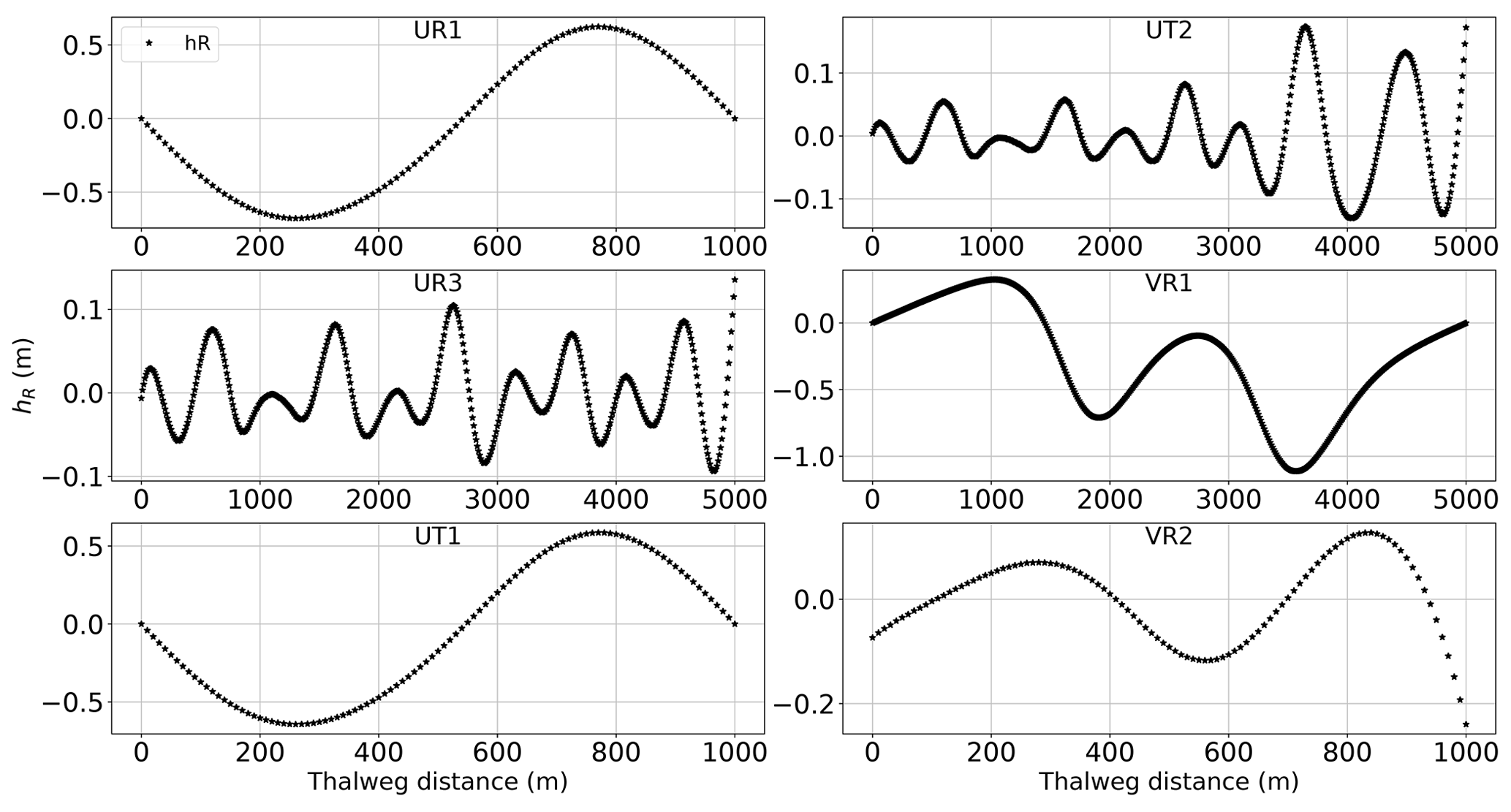
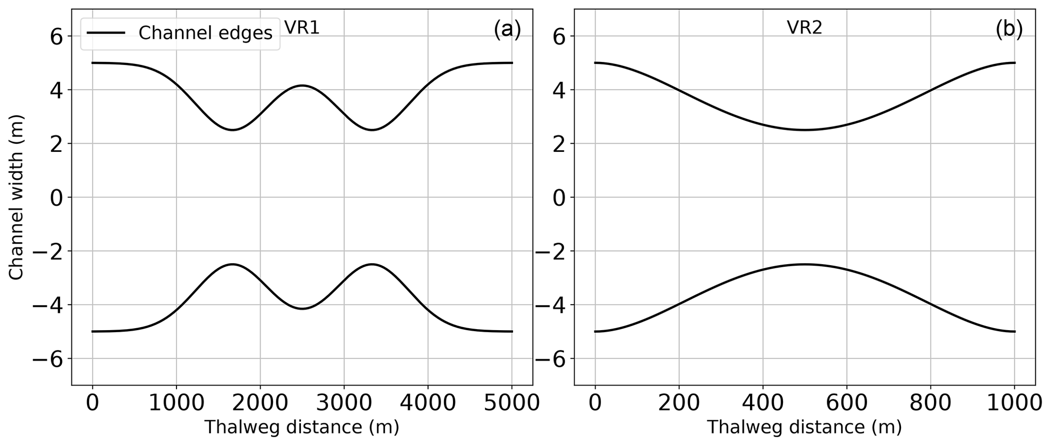
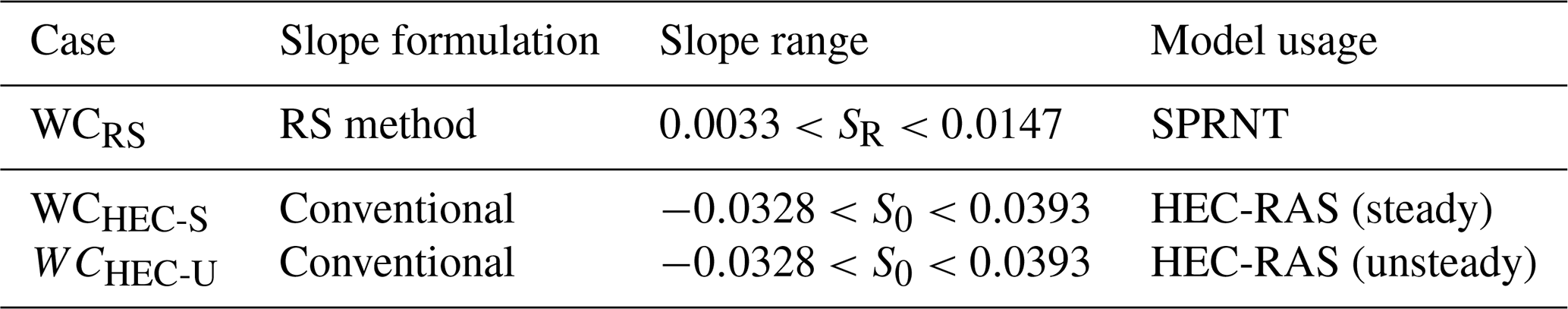
Analytical solutions of six test cases with different channel shapes and bed slope formations from MacDonald et al. (1995) are used to show that SPRNT-RS reproduces the correct water surface elevation regardless of the selection of S_R. These test cases are representative of the more comprehensive analysis provided in Yu et al. (2019a). The configuration details for each case are provided in Table 1, for which we adopt the nomenclature of MacDonald et al. (1995) for ease of comparison. The selected test cases have Lipschitz smooth geometric features that are represented in RS tests using both uniform and splined reference beds, as shown in Fig. 5. To illustrate the adaptability of the RS method, the UR3 and UT2 cases use splines that produce z_R very close to (but not identical to) the actual bed, whereas the other cases use uniform S_R or splines with greater differences. The uniform S_R in cases UR1, UT1, and VR1 is set to the average slope in each domain. With reference to Fig. 4, the differences between the channel bottom (z₀) and the reference bottom (z_R) shown in Fig. 5 imply channel bottom offsets (h_R) of varying complexity for the RS method, as shown in Fig. 6. The VR1 and VR2 cases also provide smooth changes in the channel width, which are shown in Fig. 7. The node spacing for all these tests is a uniform Δx=10 m. The boundary conditions follow MacDonald et al. (1995).

Table 1 Configuration and geometric data for analytical test cases derived from MacDonald et al. (1995). W_B and S_SW represent bottom width and sidewall slope, respectively.

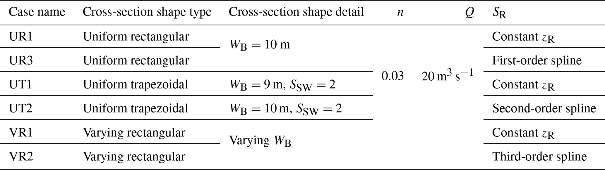
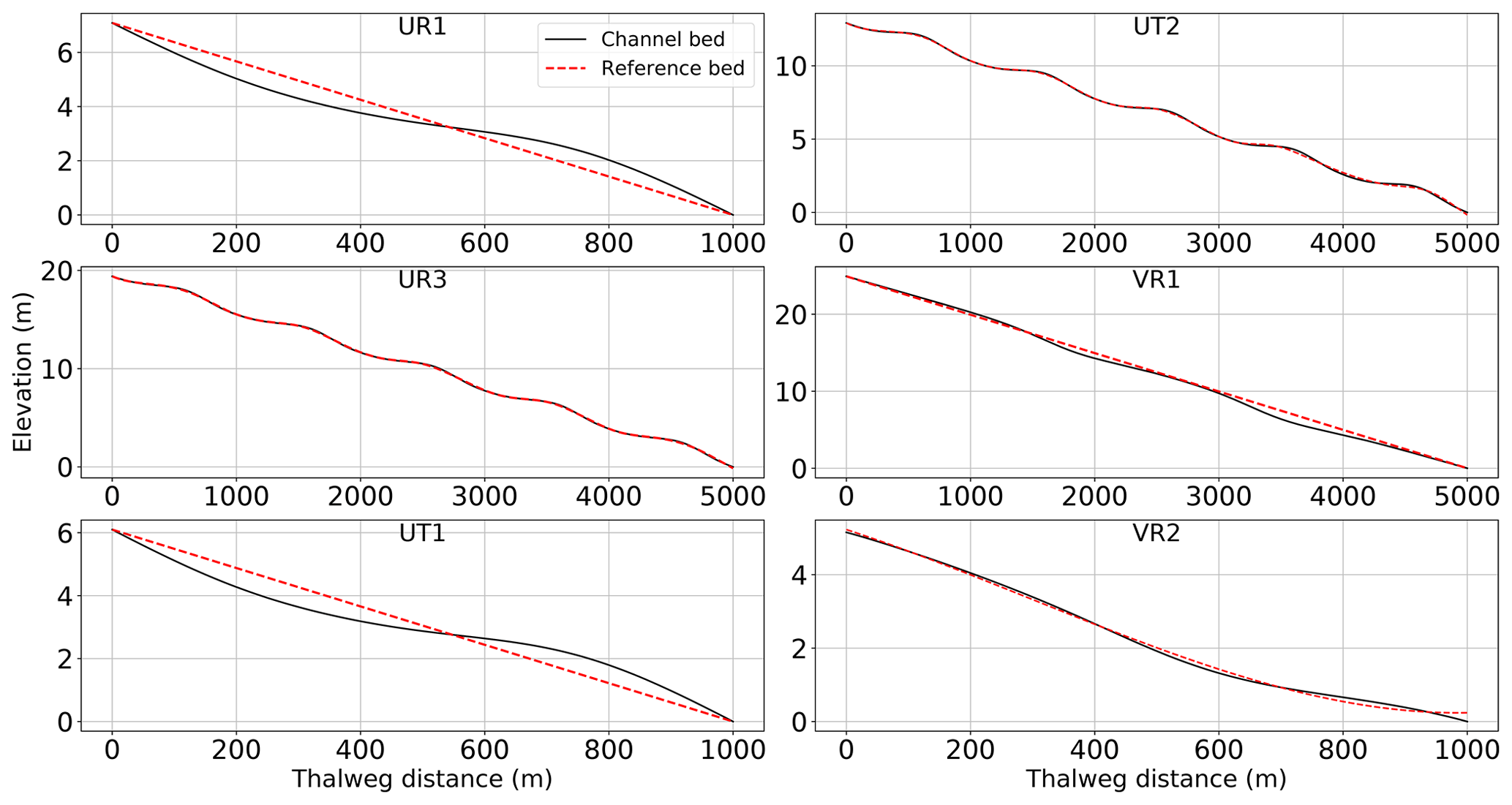
Figure 5 Channel bed elevation (z₀) and reference bed elevation (z_R) for six test cases from MacDonald et al. (1995).

Figure 6 Reference bed offset, h_R, for z_R and z₀ of the test cases in Fig. 5.

Figure 7 Plan view of channel edges for cases VR1 (a) and VR2 (b) of Fig. 5.

3.6 Test cases – synthetic channel reach

The analytical test cases above are designed to show that the RS method does not introduce approximations that affect the smooth solution. However, the true power of the RS method is in solutions of non-smooth bathymetry in which most models using h₀ and S₀ have difficulty converging. To illustrate this aspect, we use a simple river reach with a randomly perturbed (discontinuous) bathymetry at various scales. As there are no analytical solutions for these tests, we use the HEC-RAS model for comparison. The simulations use time-invariant boundary conditions with geometry defined by trapezoidal cross sections of uniform side slope, as detailed in Table 2. The channel bed offset (h_R) and thalweg slope (S₀) are illustrated in Fig. 8. The flow boundary conditions provide for a mild slope with a water surface profile that can be classified as an M1 gradually varying flow.

Case 1 is the baseline smooth channel with a uniform slope over the entire reach length. Cases 2 through 5 have a synthetic geometry developed by random perturbations of the bottom elevation of the baseline reach. Cases A and B have the identical smooth geometry to Case 1 but use different reference slopes for RS tests. The synthetic channel test reach is 1.58 km in length discretized into 80 uniform computational nodes with 79 channel segments (20 m per segment). The trapezoidal cross sections each have a 10.0 m bottom width and 63.4^∘ sidewall slopes. Bottom roughness is fixed by a Manning's n value of 0.04 for all segments.

Table 2 Configuration of synthetic channel reach test cases: α is used in Eq. (20) for random perturbation of the baseline Case 1 geometry; h_R is the bed offset based on Fig. 4 with parentheses indicating upper and lower limits of randomized geometry values over the nonuniform test reach; S₀ is the range of the thalweg slope for z₀ from Eq. (20); and S_R is the selected uniform reference slope.

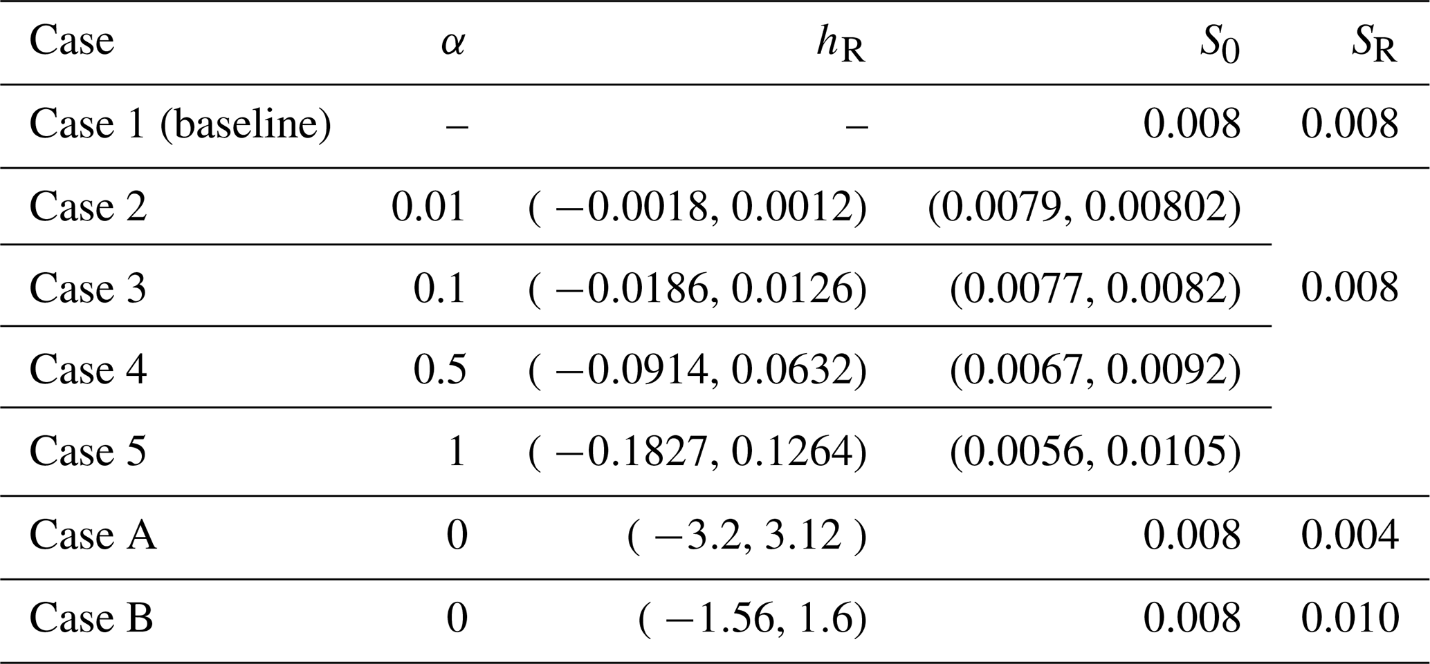
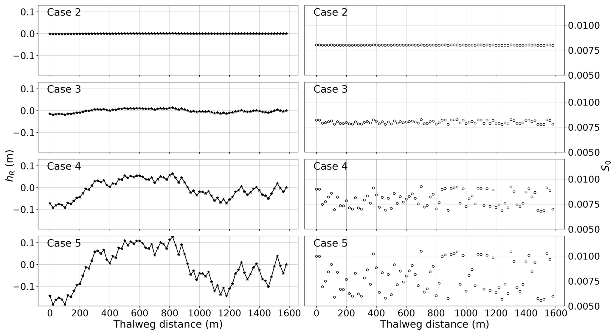
Figure 8 Channel bottom offset (h_R) and physical thalweg slope (S₀) for synthetic test cases 2–5 that are random perturbations of the baseline smooth S₀=0.008 of Case 1.

To develop the random perturbations of the bottom in the synthetic test cases, we begin with Case 1 (baseline) using a uniform $S_{\mathrm{0}}^{\left[\mathrm{1}\right]}=\mathrm{0.008}$ over the entire reach length. Here the superscript in square brackets indicates the case identifier. The set of bottom elevations for Case 1 are $z_{\mathrm{0}}^{\left[\mathrm{1}\right]}\left(x\right)$, which are smooth and linearly decreasing over the reach length. Cases 2–5 are similar channels with perturbed bottom elevations set by

$$\begin{array}{}\text{(20)}& z_{\mathrm{0}}^{\left[c\right]}\left(x\right)=z_{\mathrm{0}}^{\left[\mathrm{1}\right]}\left(x\right)+{\mathit{\alpha }}^{\left[c\right]}H\left(x\right):c\in \left\{\mathrm{2},\mathrm{3},\mathrm{4},\mathrm{5}\right\},\end{array}$$

where H(x) is a set of random-generated numbers within the range of $-\mathrm{0.126}\le H\left(x\right)\le \mathrm{0.183}$. The upper and lower limits of H(x) were selected to prevent the occurrence of a locally adverse slope – such conditions can be handled by SPRNT-RS but can cause convergence problems for some models. The α^[c] is a magnitude to generate a range of bottom displacements with ${\mathit{\alpha }}^{\left[c\right]}\in \left\{\mathrm{0.01},\mathrm{0.1},\mathrm{0.5},\mathrm{1.0}\right\}$ for $c\in \left\{\mathrm{2},\mathrm{3},\mathrm{4},\mathrm{5}\right\}$, respectively. Cases 2–5 set the reference bottom elevations exactly equal to the baseline Case 1 physical bottom elevations; i.e.,

$$\begin{array}{}\text{(21)}& z_{\mathrm{R}}^{\left[c\right]}\left(x\right)=z_{\mathrm{0}}^{\left[\mathrm{1}\right]}\left(x\right):c\in \left\{\mathrm{2},\mathrm{3},\mathrm{4},\mathrm{5}\right\}.\end{array}$$

Thus, the SPRNT-RS simulations for cases 2–5 use uniform S_R over the reach such that the bed offset (h_R) represents the physical geometric perturbations. Noting from Eq. (13) that h_R is the difference between the physical bottom ($z_{\mathrm{0}}^{\left[c\right]}$) and the reference bottom ($z_{\mathrm{R}}^{\left[c\right]}$), substituting the above relationships gives

$$\begin{array}{}\text{(22)}& h_{\mathrm{R}}^{\left[c\right]}\left(x\right)={\mathit{\alpha }}^{\left[c\right]}H\left(x\right).\end{array}$$

For synthetic test cases A and B in Table 2, the actual channel bottom slopes are set to uniform values equivalent to Case 1; that is $S_{\mathrm{0}}^{\left[A\right]}=S_{\mathrm{0}}^{\left[B\right]}=S_{\mathrm{0}}^{\left[\mathrm{1}\right]}=\mathrm{0.008}$ with identical thalweg elevations of $z_{\mathrm{0}}^{\left[\mathrm{1}\right]}\left(x\right)$. However, the reference slopes for these cases are set to smaller and greater uniform values: $S_{\mathrm{R}}^{\left[A\right]}=\mathrm{0.004}$ and $S_{\mathrm{R}}^{\left[B\right]}=\mathrm{0.010}$. These two cases demonstrate that the RS method generates the same numerical solution as baseline Case 1 (solved at S₀) when S_R is set to an arbitrary value.

Forcing for all seven test cases is a constant inflow boundary of 283 m³ s⁻¹ applied at the furthest upstream node. The downstream boundary condition is 5.0 m depth, which is a subcritical flow based on a normal depth of 4.95 m for S₀=0.008 and the inflow rate. Because a subcritical boundary condition allows upstream wave reflections, the downstream boundary was enforced at the end of a 180 m (9 node) buffer domain, which was adequate for reducing upstream wave propagation in unsteady flow solutions. Simulation results are reported after the models have reached a steady state and all oscillations associated with the initial conditions have dissipated. Solutions for the buffer segment are not included in the analyses below.

3.7 Test case – Waller Creek study site

The main stem of Waller Creek in Austin, Texas, USA, is used to examine the performance of the RS method for more complex conditions. The main stem of the creek drains an urban watershed of 14.3 km² with total length of 10.7 km for the area illustrated in Fig. 9. Bathymetric survey data are available courtesy of the city of Austin (Fig. 10). The bathymetric data set includes 327 surveyed cross sections with spacing intervals ranging from 2.5 up to 178 m (mean of 33.5 m). The Manning's n of the channel (based on the city of Austin computations) varies from 0.02 to 0.06 throughout the system. The SPRNT model, in both its original and RS form, has numerical stability issues associated with close cross-section spacing. Arguably, these issues are related to sharp changes in A that lead to non-smooth source terms despite the RS method; however, this issue requires further investigation. Similar numerical instability behavior can also be found in the HEC-RAS unsteady model and also causes divergent solutions. For the present work, we discarded 36 cross sections (11 % of the data set) that were closer than 10 m and merged these short reach lengths with the adjacent sections. An additional three cross sections were discarded and some channel roughness values were modified as they caused numerical instability in the HEC-RAS unsteady simulation (see Appendix for details). The resulting data set is 288 cross sections with spacing ranging from 10.1 to 184.9 m. The mean cross-section spacing is 37.2 m with a total reach length of 10.7 km. To limit our focus to subcritical flow, our analyses consider only the upper 8.3 km of the main reach (210 out of 288 cross sections), which eliminates a series of step-pool transcritical elements in the downstream channel in which the HEC-RAS solution is strongly influenced by the ad hoc local partial inertia (LPI) algorithm (Fread et al., 1996; Brunner, 2016b). The smoothing introduced by LPI makes it difficult to draw conclusions from a comparison between SPRNT-RS and HEC-RAS across transcritical locations.

Figure 9 Main stem of Waller Creek and catchment in Austin (Texas, USA). Basemap © by Open Geospatial Consortium (OGC) Web Mapping Service (WMS).

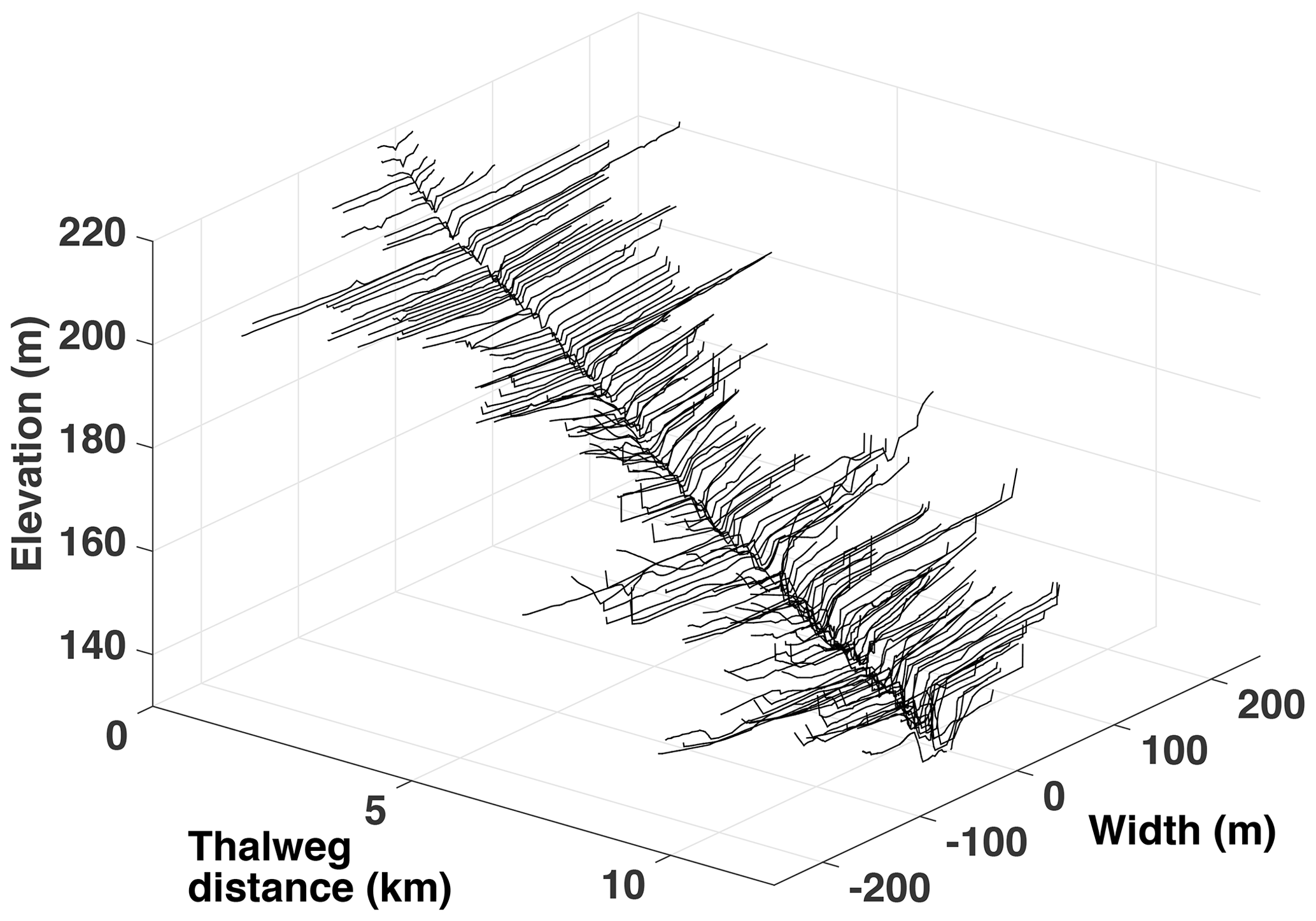
Figure 10 Surveyed cross sections of Waller Creek. Only 140 out of 327 cross sections are shown for clarity. Elevations are relative to mean sea level. Data courtesy of the city of Austin.

A time-invariant upstream inflow boundary condition is set to 25 m³ s⁻¹ at the headwater cross section. To minimize the influence of subcritical reflections from the upstream inflow boundary, the first 10 computational nodes at the upstream are not included in the results analysis. Lateral inflows are set to zero for all test cases. A 300 m buffer section is added downstream of the test domain to reduce the influence of reflections from the downstream boundary condition. This buffer section uses the same cross section as the final downstream section of the data set with a bed slope (S₀) of 0.0033 and Manning's n of 0.04. The buffer section has a normal depth of 0.76 m at the 25 m³ s⁻¹ inflow rate. The downstream boundary condition at the end of the buffer section is 0.7 m depth, which is subcritical and implies an M2 gradually varying drawdown in the vicinity of the outflow. These geometry and boundary conditions are identically applied to both SPRNT-RS and HEC-RAS models.

The thalweg elevation, z₀(x), and the reference elevation, z_R(x), of the RS method (as determined by the approximate spline fit described above) for Waller Creek are shown in Fig. 11a. The z₀ and z_R are visually similar with the former being somewhat more noisy. The elevation data sets provide similar overall reach slopes (uppermost cross section to lowermost cross section) of 0.0074 and 0.0077, respectively. Note that the approximate B-spline technique for generating z_R(x) does not force the overall reach slope to be identical. Because z_R(x) is mathematically arbitrary, there is no need to force an exact match. Although z₀(x) and z_R(x) are similar in Fig. 11a, S₀(x) from the raw data is discontinuous and varies over a wide range (up to 4 times the reach slope), as illustrated in Fig. 11b. Note that S₀(x) also includes negative slopes (i.e., adverse gradient sections) which can cause convergence problems for some numerical solvers. In contrast, as shown in Fig. 11c, the approximate cubic B-spline used to generate S_R(x) from z_R(x) provides a reference slope that is everywhere smooth and positive and remains close to the overall reach slope of 0.008. The slope range and model nomenclature for the Waller Creek test cases are provided in Table 3. The Lipschitz smoothness of S₀ versus S_R can be better understood by evaluating the gradient of the slope, i.e., the second derivative of z₀ and z_R, as shown in Fig. 11d. The S₀ formulation clearly lacks smoothness in the higher derivative.

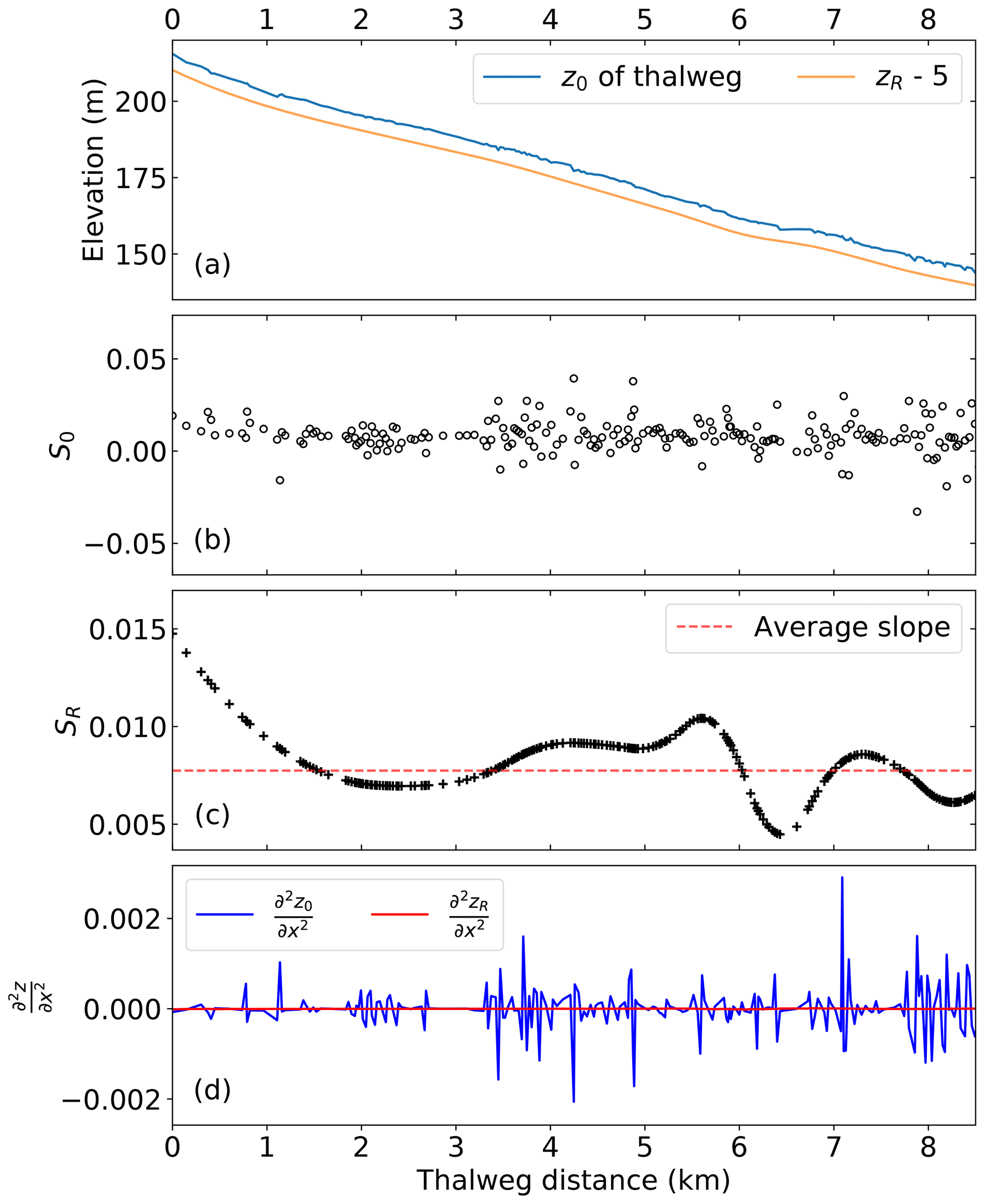
Figure 11 Waller Creek bottom elevation and slope: (a) z elevation, with 5 m subtracted from z_R for clarity; (b) S₀ thalweg slope between cross sections; (c) S_R smoothed bottom slope; and (d) second derivative of z₀ and z_R. Note the y-axis scaling in (c) has reduced limits compared to (b) to better show the smoothness achieved by the spline fit.

Table 3 Data for model setup of Waller Creek test cases.

3.8 Analysis methods

To evaluate the performance of the RS method relative to conventional formulations, four depth-based indicators are employed, as described below. For these definitions, the control (superscript [C]) is the MacDonald et al. (1995) solution for the analytical test case and HEC-RAS results for the synthetic channel and Waller Creek test cases. Note that the synthetic tests use unsteady HEC-RAS, whereas the Waller Creek study uses comparisons to both steady and unsteady versions of the model. The test case (superscript [T]) is always the SPRNT-RS simulation. These measures can be considered error metrics for the comparison to the analytical solutions and difference metrics for model–model comparisons.

1. Normalized difference (ρ). A nondimensional index to describe the local difference in depth can be defined as

   $$\begin{array}{}\text{(23)}& {\mathit{\rho }}^{[T:C]}\left(x\right)={\displaystyle \frac{h_{\mathrm{0}}^{\left[C\right]}\left(x\right)-h_{\mathrm{0}}^{\left[T\right]}\left(x\right)}{h_{\mathrm{0}}^{\left[C\right]}\left(x\right)}},\end{array}$$

   where $h_{\mathrm{0}}^{\left[C\right]}\left(x\right)$ and $h_{\mathrm{0}}^{\left[T\right]}\left(x\right)$ are the local depth solutions from the control and test case results after steady-state conditions are achieved. The normalization scale is the local depth of the control case. Note the denominator is nonzero in the synthetic test case setup because the flow setup is an M1 gradually varying flow.

2. Absolute mean normalized difference (ζ). The mean of the absolute value of ρ(x) over the domain provides an overall nondimensional indicator of the depth error:

   $$\begin{array}{}\text{(24)}& {\mathit{\zeta }}^{[T:C]}={\displaystyle \frac{\mathrm{1}}{N}}\sum _{x=\mathrm{1}}^N\mid {\mathit{\rho }}^{[T:C]}\left(x\right)\mid ,\end{array}$$

   where N is the total number of cross sections. We use the absolute value so that positive errors do not cancel negative errors, and ζ is a representative scale of the discrepancy between models.

3. Mean absolute error (MAE). The overall dimensional error is characterized as

   $$\begin{array}{}\text{(25)}& \text{MAE}={\displaystyle \frac{\mathrm{1}}{N}}\sum _{x=\mathrm{1}}^N\mid h_{\mathrm{0}}^{\left[C\right]}\left(x\right)-h_{\mathrm{0}}^{\left[T\right]}\left(x\right)\mid ,\end{array}$$

   and the nondimensional form of overall error is

   $$\begin{array}{}\text{(26)}& \begin{array}{rl}\text{MAE}& \text{(nondimensional)}\\ & ={\displaystyle \frac{\mathrm{1}}{N}}\sum _{x=\mathrm{1}}^N\mid {\displaystyle \frac{h_{\mathrm{0}}^{\left[C\right]}\left(x\right)-h_{\mathrm{0}}^{\left[T\right]}\left(x\right)}{h_{\mathrm{0}}^{\left[C\right]}\left(x\right)}}\mid .\end{array}\end{array}$$

4. Root mean square error (RMSE). A standard dimensional measure of the squared error is

   $$\begin{array}{}\text{(27)}& \text{RMSE}=\sqrt{{\displaystyle \frac{\mathrm{1}}{N}}\sum _{x=\mathrm{1}}^n\left(h_{\mathrm{0}}^{\left[C\right]}\right(x)-h_{\mathrm{0}}^{\left[T\right]}(x){)}^{\mathrm{2}}}.\end{array}$$

   The nondimensional form of RMSE is computed by the following equation:

   $$\begin{array}{}\text{(28)}& \begin{array}{rl}\text{RMSE}& \text{(nondimensional)}\\ & =\sqrt{{\displaystyle \frac{\mathrm{1}}{N}}\sum _{x=\mathrm{1}}^n({\displaystyle \frac{h_{\mathrm{0}}^{\left[C\right]}\left(x\right)-h_{\mathrm{0}}^{\left[T\right]}\left(x\right)}{h_{\mathrm{0}}^{\left[C\right]}\left(x\right)}}{)}^{\mathrm{2}}}.\end{array}\end{array}$$

   Both the MAE and RMSE are also reported in nondimensional form where the normalization scale is presented.

4 Results

4.1 Analytical test cases

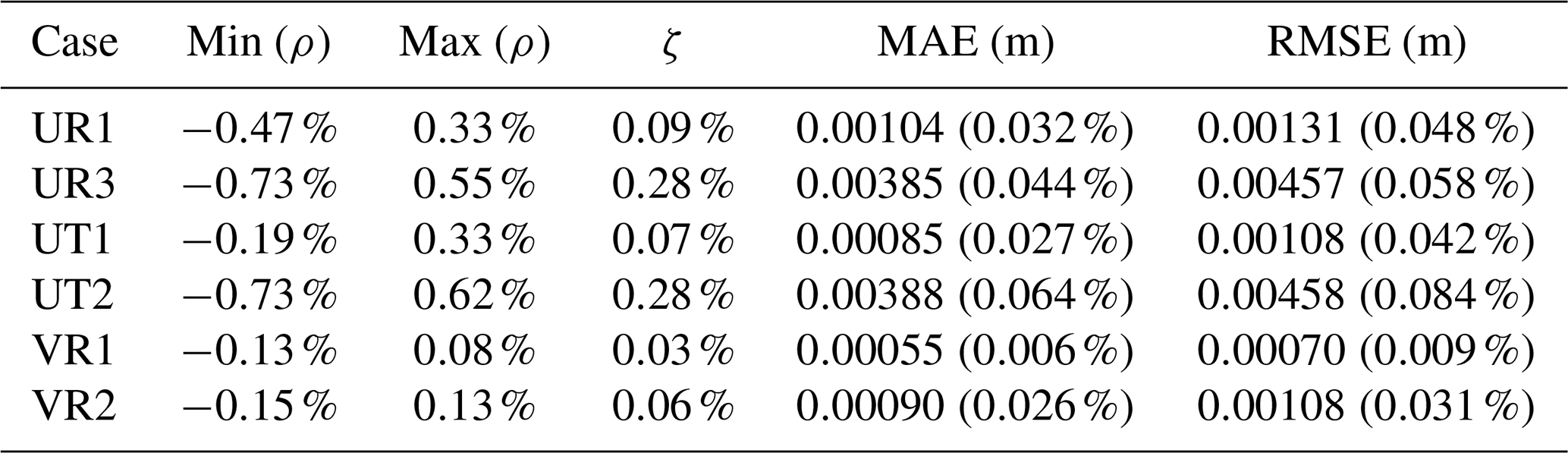
The water surface elevations for the analytical solutions and SPRNT-RS simulations are shown in Fig. 12. Visually, the analytical and simulated results across all six cases are identical. Error metrics following Sect. 3.8 are provided in Table 1. The normalized differences (ρ) are less than 1 % and are consistent with absolute errors of O(10⁻³) m, which are negligible compared with the water depths ≥1 m. The spatial distributions of the normalized error are shown in Fig. 13. By comparing this figure with Fig. 5, it can be seen that ρ(x) fluctuates with the change in bed slope. Similar behavior can also be found for model results reported in MacDonald et al. (1995).

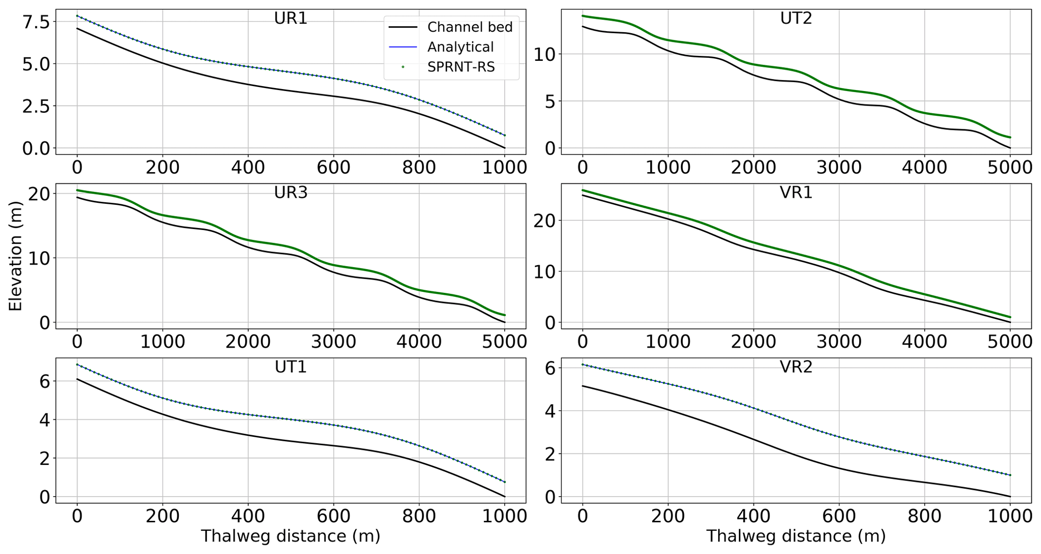
Figure 12 Comparison between simulated water surface elevation from SPRNT-RS and analytical solution for analytical test cases of MacDonald et al. (1995).

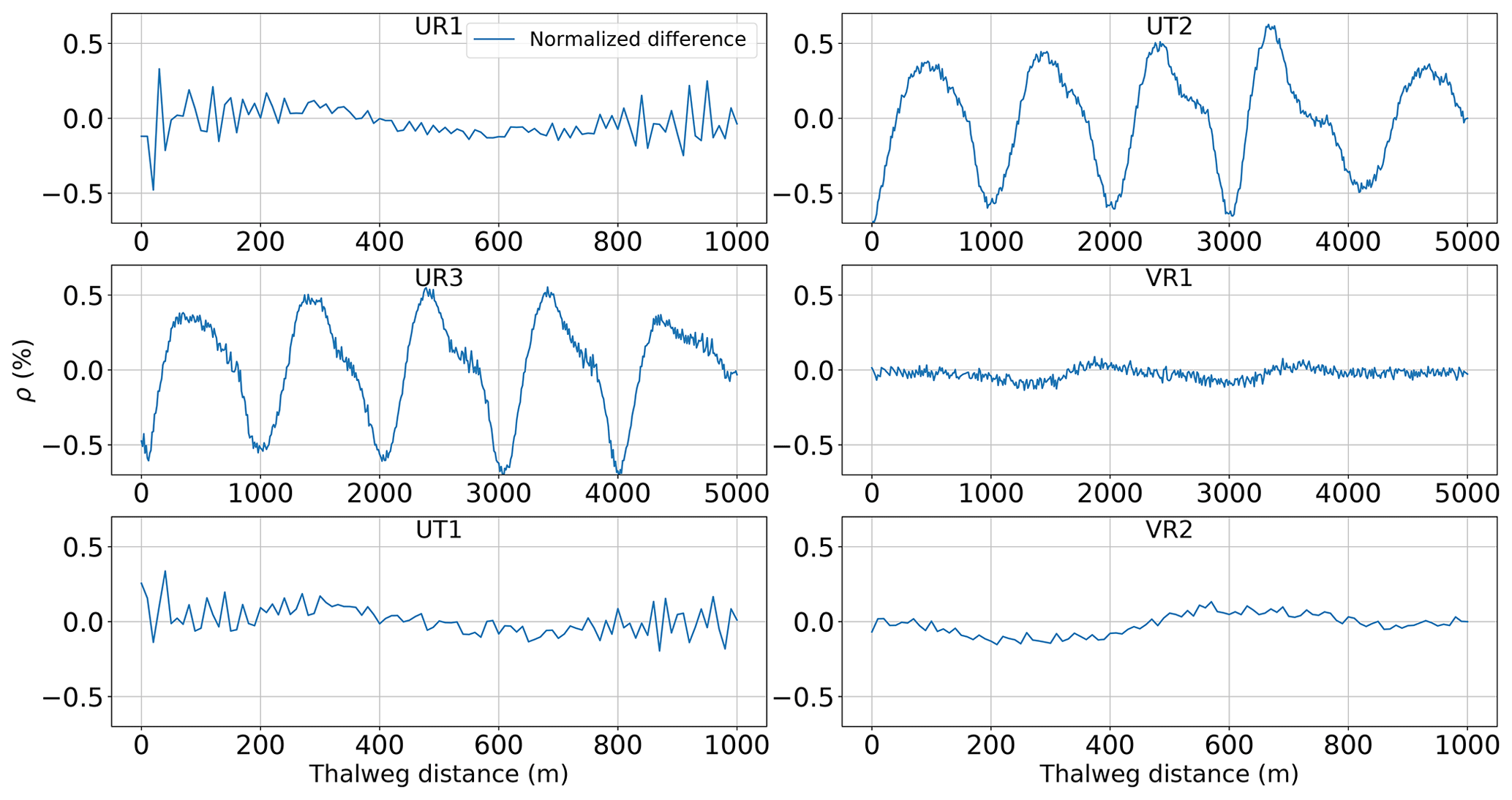
Figure 13 Spatial distribution of normalized difference (ρ) for analytical test cases of MacDonald et al. (1995).

Table 4 Difference measures using Eqs. (23)–(28) for analytical test cases of MacDonald et al. (1995). Nondimensional MAE and RMSE are shown in parentheses.

4.2 Synthetic test cases

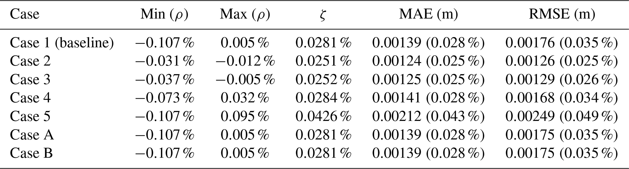
Results for the baseline synthetic test, Case 1, are shown in Fig. 14. The SPRNT-RS method produces visually the same solution to HEC-RAS with z_R=z₀. Similarly, the comparison of model results for depth (h₀) for test cases 2–5 are visually indistinguishable, as shown in the left column of Fig. 15. The quantitative difference measures for the synthetic tests are provided in Table 5, and the spatial distributions of ρ(x) are illustrated in the right column of Fig. 15. Values for ρ(x) in cases 2 and 3 are slightly below zero (≈0.02 %) over the entire domain, indicating the SPRNT-RS solution has a slightly higher water surface than the HEC-RAS solution for small perturbations in the bed slope. With the increased bottom perturbations in cases 4 and 5, the ρ(x) range is larger (and includes a positive range), but the bounding values are still trivial. The ζ and RMSE measures show that the nondimensional and dimensional overall differences are small. The MAE and RMSE climb slightly with the increasing h_R for cases 2 through 5 but remain below 3 mm. These depth RMSE values are negligible compared with the normal depth (4.95 m) of the baseline and well within reasonable truncation error differences for solvers using different numerical techniques. The model–model comparisons for test cases A and B also have trivial errors (Table 5), and further results are not shown as they are visually identical to those for baseline Case 1 illustrated in Fig. 14. Note that the RMSE for both cases is identical to Case 1, which indicates the solution for the SPRNT-RS method with S_R≠S₀ is very close to the baseline solution with S_R=S₀.

Figure 14 Simulated profile of water surface elevation (upper line) and channel bottom (lower line) for synthetic test Case 1 using SPRNT-RS (red) and unsteady HEC-RAS (black).

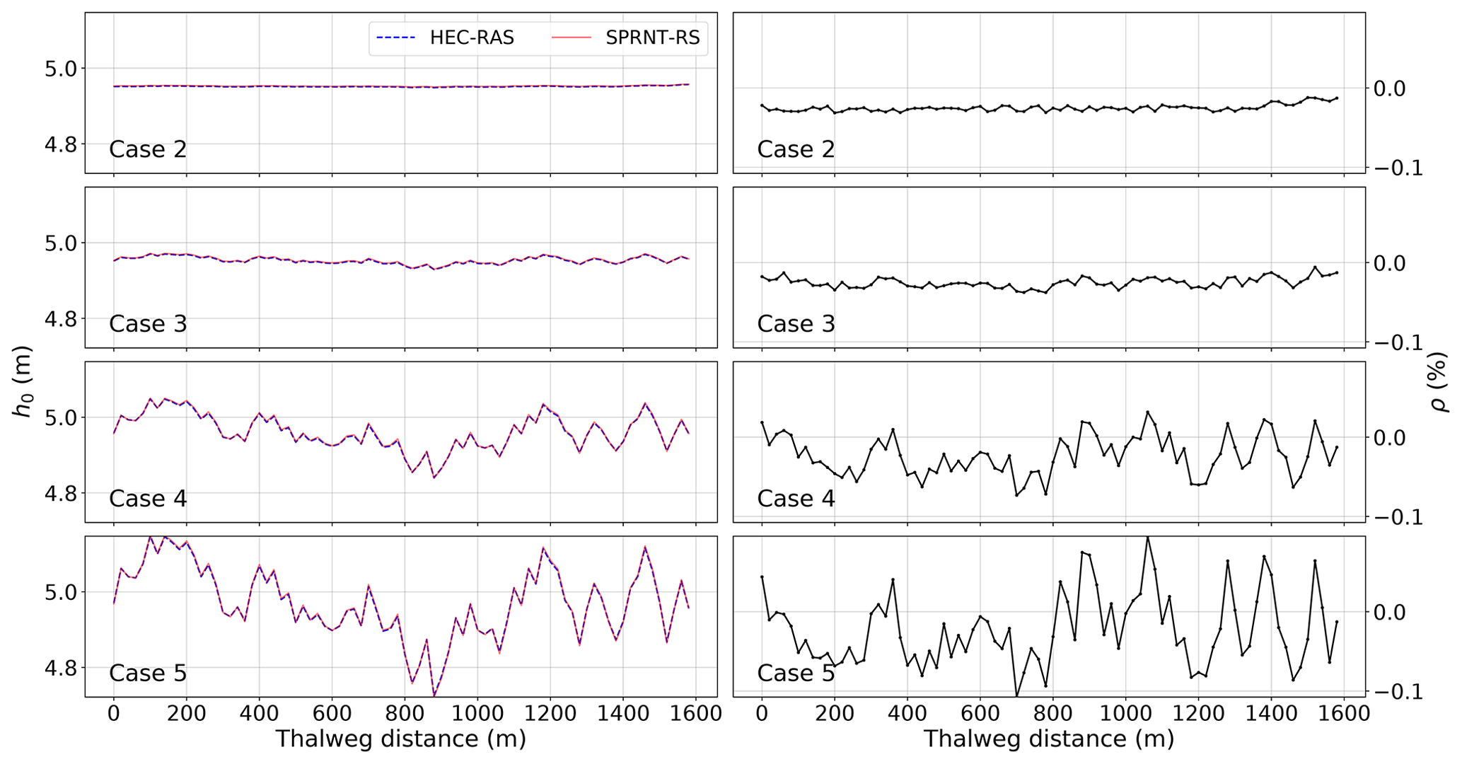
Figure 15 Water depth, h₀, (left column) and normalized difference, ρ, (right column) for synthetic test cases with perturbed bathymetry.

Table 5 Difference measures between SPRNT-RS and HEC-RAS using Eqs. (23)–(28) for synthetic test cases. Nondimensional MAE and RMSE are shown in parentheses.

4.3 Waller Creek test case

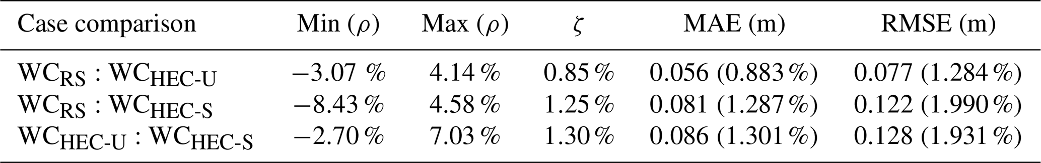
Waller Creek has been simulated with SPRNT-RS (denoted as WC_RS in the following figures), the HEC-RAS unsteady solver (WC_HEC-U), and the HEC-RAS steady solver (WC_HEC-S). Figure 16 shows water surface elevations for SPRNT-RS and unsteady HEC-RAS. For clarity, the upper 40% of the domain (which has similar good behavior) is not shown. Figure 17 shows the spatial distribution of the normalized difference, ρ, for these simulations. The differences are roughly within ±4 % across the entire domain. The maximum and minimum difference both occur at two adjacent nodes close to 7800 m with 4.14 % and −3.07 %, respectively. Figure 18 provides a similar comparison of water surface elevations between SPRNT-RS and the steady HEC-RAS case. The results are visually quite similar to the comparison with unsteady HEC-RAS. A direct comparison of surface elevations for unsteady and steady HEC-RAS does not provide any further insight and is omitted for brevity. However, to quantitatively evaluate the differences between SPRNT-RS and HEC-RAS, it is useful to compute difference measures between the unsteady and steady HEC-RAS models themselves, as well as the differences between SPRNT-RS and both models, as provided in Table 6. Overall, the SPRNT-RS result have marginally better consistency with unsteady HEC-RAS than with steady HEC-RAS. Of greater importance is that the behavior of SPRNT-RS relative to unsteady HEC-RAS has the same order of differences as the comparison of unsteady HEC-RAS to steady HEC-RAS. These results imply that the differences between SPRNT-RS and unsteady HEC-RAS are reasonable for the different numerical methods given the geometric variability of Waller Creek.

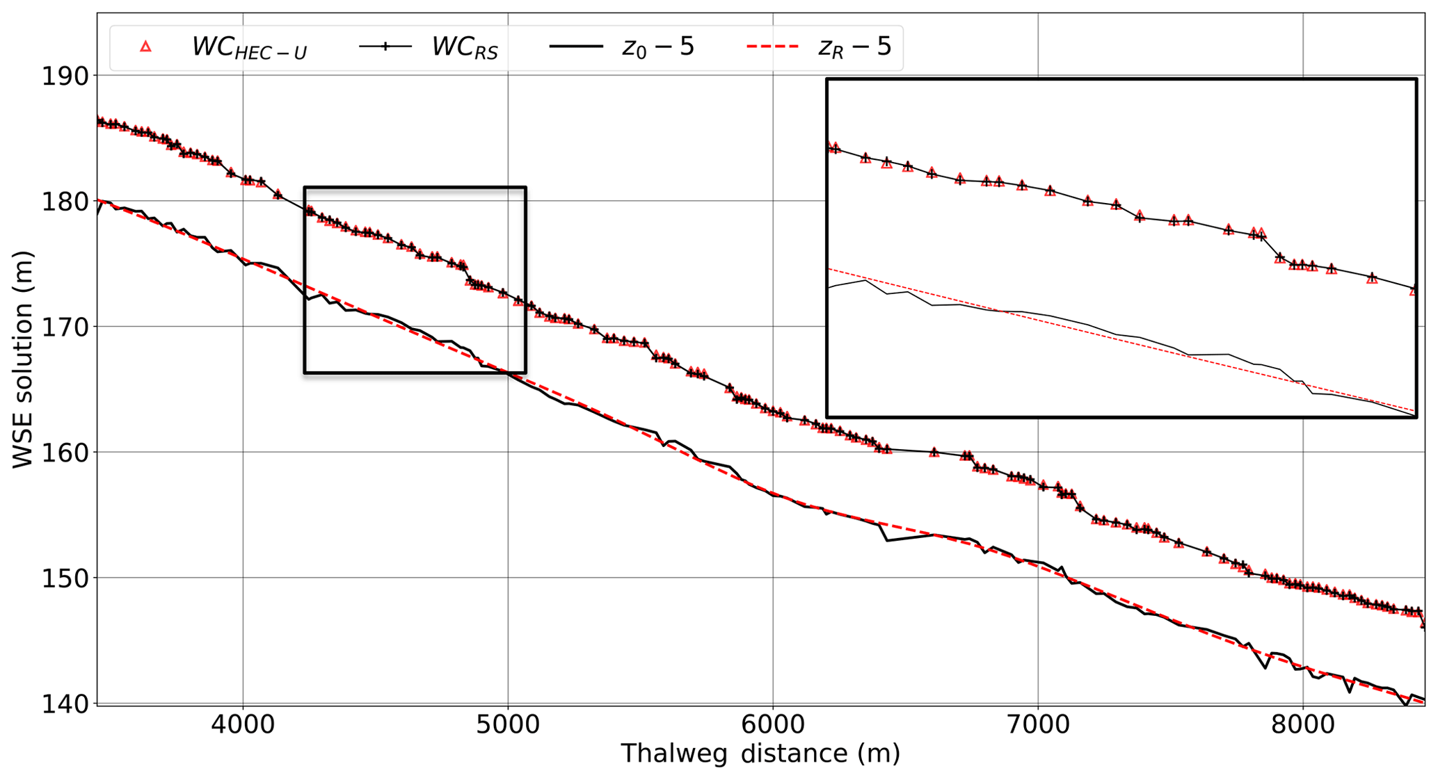
Figure 16 Comparison of SPRNT-RS to unsteady HEC-RAS for water surface elevations in Waller Creek simulations with expanded detail to show similarities. For clarity, 5 m is subtracted from the channel z elevations.

Figure 17 Normalized difference ρ(x) between SPRNT-RS and unsteady HEC-RAS.

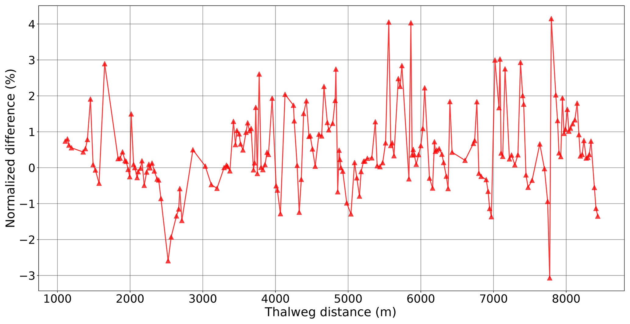
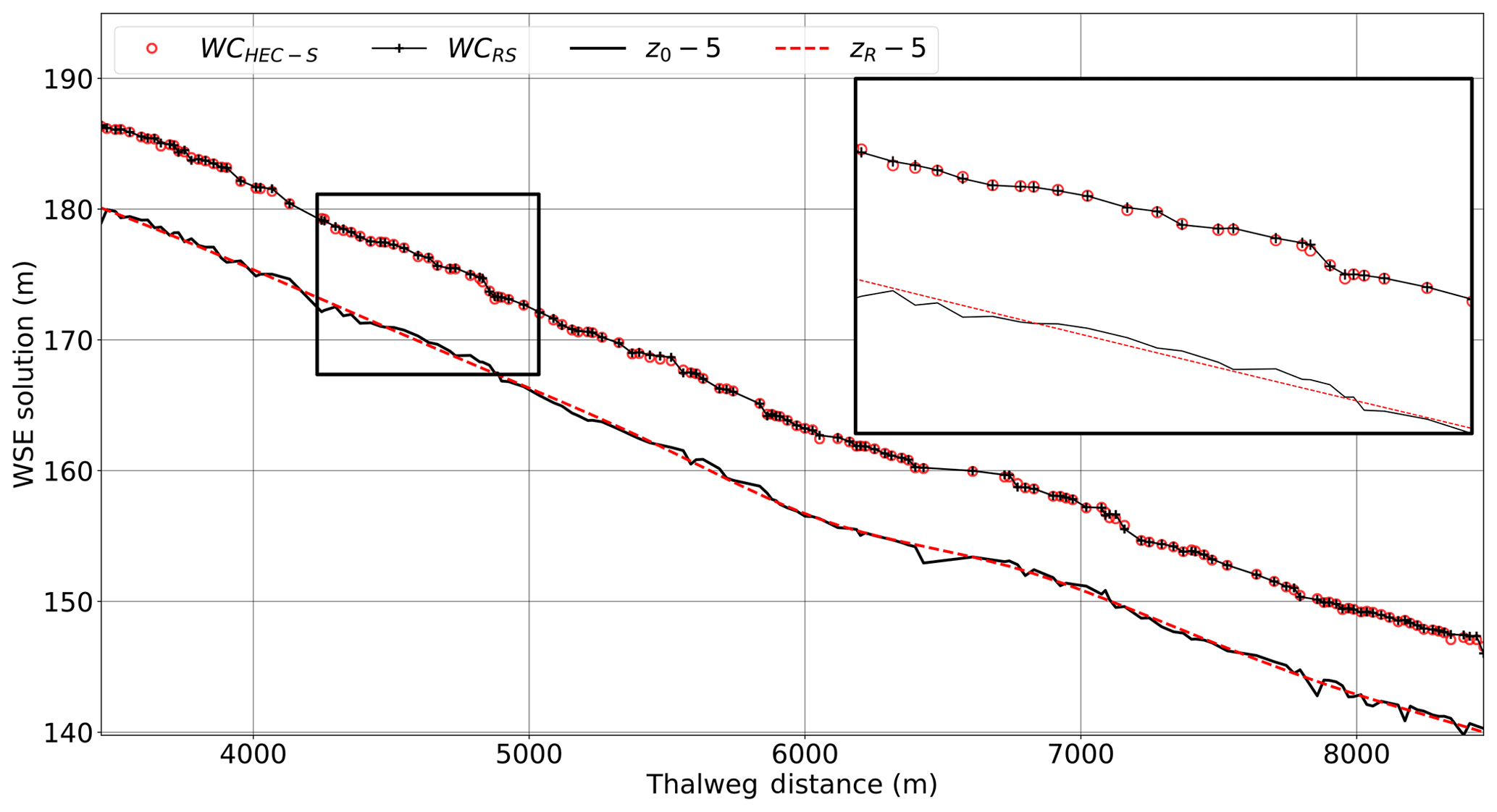
Figure 18 Comparison of SPRNT-RS to steady HEC-RAS for water surface elevations in Waller Creek simulations with expanded detail to show similarities. For clarity, 5 m is subtracted from the channel z elevations.

Table 6 Difference metrics for Waller Creek simulation results. Nondimensional MAE and RMSE are shown in parentheses.

5 Discussion

5.1 Validation of the RS method

The RS method is a simple algebraic transformation of the governing equations, and the answer to the principal question “does it work” is implied by our inability use the baseline SPRNT model (with S₀) as a control model (see Sect. 3.4). Invariably, discontinuous topography for SPRNT without RS caused either an oscillatory solution or numerical instability. In contrast, both HEC-RAS (using η) and SPRNT-RS (using S_R) provide stable, non-oscillatory solutions.

The analytical results in Sect. 4.1, supplemented by additional results in Yu et al. (2019a), validate the SPRNT-RS method for the simulation of smoothly varying channel morphologies that are Lipschitz continuous at the discretization scale. We have experimented with both uniform and splined S_R for these tests. For both types of simulations, we observe errors relative to physical experiments that are comparable or smaller than those shown in the numerical validation studies of MacDonald et al. (1995). These results imply that the transformation from the conventional h₀ and S₀ form of the SVEs to the h_a and S_R form of Eq. (17) is a valid algebraic step that can be implemented in a numerical solver and is an alternative for representing smooth geometries.

The synthetic test cases in Sect. 4.2 serve two purposes. Firstly, cases A and B compared to baseline Case 1 show that the numerical solution does not depend on a particular choice of S_R. The arbitrary selection of an S_R≠S₀ results in identical solutions to S_R=S₀. Secondly, the synthetic test cases show that the SPRNT-RS method can be applied with non-smooth geometry at the discretization scale (i.e., random perturbations of the physical bottom slope), which caused non-convergent behavior in the baseline SPRNT model. As a control, we have compared SPRNT-RS with the accepted HEC-RAS model that remains stable for these test cases as it is solved with the piezometric pressure gradient rather than splitting into S₀ and the gradient of h₀. The results indicate that SPRNT-RS provides numerical solutions that are nearly identical to HEC-RAS for the non-smooth geometry test cases. Thus, using a Lipschitz smooth S_R provides a stable numerical solution for non-smooth geometry without altering the physical representation of non-smooth geometry.

The Waller Creek test case in Sect. 4.3 provides a more challenging comparison of SPRNT-RS to HEC-RAS. For this test case, the geometry discontinuities include adverse slopes and local S₀ that are ±400 % of the reach-average slope, which contrasts with perturbations of ±30 % used in the synthetic test cases of Sect. 4.2. Again, SPRNT-RS is shown to be close to the unsteady HEC-RAS solution. The model differences are within reasonable ranges, as illustrated by the fact that they are similar to the differences between HEC-RAS steady and unsteady versions. Nevertheless, it remains possible that the minor differences between HEC-RAS and SPRNT-RS are caused by a latent defect in coding the RS method or in SPRNT itself, but it is difficult to envision how such a defect could occur without also appearing in the analytical and synthetic test cases. A simpler and more compelling explanation is with the linear approximations used in unsteady HEC-RAS that are not present in SPRNT-RS. Specifically, Brunner (2016a) notes that for computational efficiency and to reduce “troublesome convergence problems at discontinuities in the river geometry,” the unsteady HEC-RAS code uses a linearization technique developed by Liggett (1975) and Chen (1973) – note that the latter document is cited by Brunner (2016a) but was not available to us. It seems likely that strong geometry discontinuities in the Waller Creek test case would be affected by this linearization, which arguably would lead to artificial smoothing of the water surface profile by HEC-RAS. Unfortunately, we do not have direct access to the HEC-RAS code and thus rely on the discussion of HEC-RAS stability in the literature (Hicks and Peacock, 2005; Sharkey, 2014) and the methodology in HEC-RAS manuals (Brunner, 2016a, b).

5.2 Why not just use $\partial \mathit{\eta }/\partial x$?

One might wonder whether S_R or S₀ is at all necessary when we could clearly just retain $\partial \mathit{\eta }/\partial x$ in the SVEs rather than using any split form. To understand the value of S_R, it is worth considering why S₀ is presently used. We have not been able to determine exactly when S₀ was first used with the SVEs, but from a hydrology viewpoint S₀ provides consistency between kinematic wave solutions (which use S₀=S_f) and the SVEs. Thus including S₀ is a logical step when considering reduced-physics approaches (Di Baldassarre, 2012). Arguably, a well-chosen S_R that matches the large-scale S₀ will serve the same purpose. The S₀ approach is also favored in models that are built on a “conservative” SVE form in which the hydrostatic pressure portion of the piezometric head gradient is abstracted into the advective gradient term (e.g., Sanders, 2001; Kesserwani, 2013). For these model, the advantage of the S₀ form is that, when S₀ equals 0 and S_f equals 0, the momentum equation can be written as a classic 1D homogenous advection equation, which is mathematically appealing. Our work in progress indicates that the S_R approach could be similarly adapted for a conservative form of the SVEs, but this issue remains speculative.

Although the utility and simplicity of the η approach is obvious, it has a key disadvantage when applied in large-scale simulations. Over large distances the free surface is monotonically increasing upstream, which has consequences for employing implicit or semi-implicit numerical solutions in a continental river dynamics framework (Hodges, 2013). Briefly, when modeling a river system from an estuary (η∼0 m) to mountain headwaters (η∼10³ m), the solution variable, η, nominally covers 3 orders of magnitude. Furthermore, as local variations on the order of 10⁻² m affect the hydrostatic pressure gradient, the solution of η requires precision over at least 5 orders of magnitude – i.e., a stiff numerical solution that can be difficult to converge for either a linear or nonlinear solver. Thus, splitting $\partial \mathit{\eta }/\partial x$ into a down-slope body force (S_R) and a local residual ($\partial h_{\mathrm{a}}/\partial x)$ is effectively removing a large-scale gradient from the solution variables, which will generally improve numerical behavior.

Despite the above disadvantages, the η form retains some advantages in creating conservative finite-volume formulations of the Saint-Venant equations (Hodges, 2019). Arguably, such methods should be confined to explicit time-marching schemes or localized solutions, in which η covers a smaller range, and the RS method should be preferred for larger systems.

5.3 RS advantages and limitations

The fundamental difference between the SPRNT-RS approach and most, if not all, conventional models (including unsteady HEC-RAS) is that our method algebraically revises the Saint-Venant equations to exactly accommodate discontinuous geometry while maintaining a smooth source term, whereas other models typically introduce ad hoc changes (e.g., linearization) to provide stable and faster numerical behavior when discontinuities are likely to cause numerical instabilities. These differences in the governing equations can be expected to cause differences in the solution – especially where nonlinear terms are strong. The present scope is limited in that only a single model was modified (SPRNT/SPRNT-RS) and only a single model (HEC-RAS) was used as an external control. The validity of the underlying algebraic transformation in the RS method has been demonstrated by these tests; however, it remains to be seen how implementing the RS approach in other models – particularly well-balanced models – might alter residual errors, convergence rates, and computational performance. We are interested in collaborating with other researchers who have access to and familiarity with source code of candidate well-balanced models.

An important limitation to the present work is that we focus solely on subcritical flow. The Preissmann scheme used in the underlying SPRNT model is known to exhibit instabilities with transcritical flows (Samuels and Skeels, 1990; Sart et al., 2010; Meselhe and Holly, 1997), which can be suppressed with the ad hoc local partial inertia (LPI) scheme of Fread et al. (1996). Our preliminary work (not shown) indicates that the RS approach can stabilize the Preissmann scheme without using LPI, but further work is required to test and validate the RS method for transcritical and supercritical flows.

Overall, the RS method can ensure the Lipschitz smoothness of slope representation in the momentum source term (without smoothing geometry), thus reducing one source of oscillatory or unstable behavior in numerical solutions. However, application of the RS method is not without some limitations. Although the switch from S₀ to S_R is algebraically exact, the application of the RS method requires some method to select the distributed z_R(x) and to determine S_R(x). Poor selection of z_R can theoretically result in non-smooth S_R. In the present work, the profile of z_R in the Waller Creek case is generated by the cubic B-spline technique, which is controlled by the number of knots and their spacing. In general, the distance between knots must be longer than the spacing between cross sections so that the generated S_R is smooth at the model's discretization scale. It is not clear that a mathematical “optimum” for selection of knots will necessarily exist, but there are likely (unknown) practical limits on knot selection spacing for “adequate” smoothness of z_R(x). Our results indicate that approximating cubic B-splines is adequate for producing smooth z_R for the tested geometries and that the solutions are robust for the selection of z_R as long as S_R is smooth (Yu et al., 2019b). However, it is likely there are limitations to applying the RS method in large-scale river network simulations that will make it difficult to use a simple globally applied knot spacing. Such networks might consist of 10⁴ to 10⁵ reaches spanning wide geographical regions with a variety of topology and inconsistent data availability. Some reaches may have well-defined cross sections at close spacing, other reaches might be poorly documented (Hodges, 2013). Thus, it seems likely that a method for automatically generating approximating splines (or some other form of smoothing) would be useful, but such an advance arguably requires a method for quantitatively evaluating the goodness of a particular set of z_R(x), which remains an open question. We speculate that simple window filtering techniques may be adequate for river databases such as NHDplus (United States National Hydrography Dataset Plus), but further investigation and examination are needed to better understand the interplay between the smoothing scales and the numerical solution using the RS method for large networks.

This study has implemented RS only in the SPRNT code, as discussed in more detail in Sect. 3. The baseline governing equations for SPRNT are of the form of Eq. (2), the so-called “nonconservative” form, which simply means that the entirety of the hydrostatic pressure gradient is effectively a source term, in contrast to “conservative” equations such as the Cunge–Liggett form (Cunge et al., 1980), in which a portion of the hydrostatic pressure gradient is abstracted to the advection term. Although it remains to be shown in future work, the algebraic transformation implied in Eq. (4) can arguably be applied in the Cunge–Liggett form or any other conservative form of the SVEs. Similarly, the fundamental algebraic transformation to S_R and $\partial h_{\mathrm{a}}/\partial x$ will be equally valid in any finite-volume method using S₀ and h₀.

The greatest barrier to the adoption of the RS method in an existing model is likely the need to rewrite the geometry functions to accept h_a, h_R, and z_R in place of h₀ and z₀. The difficulties involved in this effort depend on whether or not the model geometry functions are sufficiently isolated from the main solution algorithm. Indeed, we can imagine codes where the geometry functions are essentially dispersed throughout and require extensive effort to alter, debug, and verify.

5.4 The future for RS methods

The RS method as introduced above might be just a starting point. Although the present work focused on the nonconservative form, the concepts presented herein will likely be effective in addressing the well-balanced problem for conservative forms as reviewed in Kesserwani (2013) and Hodges (2019). Furthermore, the algebra in the RS demonstration above leads to the conjecture that the method could be extended to 2D reference slopes for bathymetry in 2D or 3D models. Undoubtedly there are unknown numerical challenges in extending to higher dimensions – particularly in ensuring a 2D spline function is adequately spaced to ensure smoothness – but there does not appear to be any fundamental conceptual difficulty in such efforts.

6 Conclusions

The reference slope (RS) method introduces a new form of the Saint-Venant equations for 1D river flow. The advantage of the RS method is that it ensures the body force (slope) source term is smooth and cannot destabilize the numerical solution. The RS method introduces the concept of an arbitrary smooth reference elevation, z_R(x), with computed reference slopes, S_R(x), and associated depths, h_a(x). These geometries are algebraically related to the traditional channel thalweg elevation, depth, and bottom slope ($z_{\mathrm{0}},h_{\mathrm{0}},S_{\mathrm{0}}$) used in many models. The RS method is implemented in an open-source Saint-Venant solver as SPRNT-RS. In this study, SPRNT-RS was compared to both analytical solutions and the conventional HEC-RAS model for synthetic test reaches and an urban creek for subcritical flows. The model–model comparisons are within the expected truncation error for both the analytical and synthetic test cases and within acceptable differences for simulating flow through the complex geometry of an urban creek. The slightly larger simulation differences in the urban creek test case are likely due to ad hoc linearization algorithms used in HEC-RAS that do not appear in SPRNT-RS.

As discussed in the Sect. 2, when faced with non-smooth geometries in a channel reach, prior researchers have resorted to limiting or smoothing discontinuous source terms or employing numerical techniques that mitigate oscillatory/unstable numerical behaviors. In contrast, the new RS method transforms a discontinuous bottom slope source term into a smooth expression without losing either complexity in the geometry or introducing ad hoc smoothing of the geometry, the numerical method, or the solution. An important advantage of the RS method is that it is entirely mechanical, requiring only the selection of control knot spacing for the approximating spline at some length scale larger than the cross-section spacing. That is to say that RS does not require the model designer or user to introduce smoothing thresholds or ad hoc algorithm bounds. As such, we believe the RS method could be particularly valuable as we move from fine-resolution reach-scale modeling to large-scale continental river dynamic simulations (Hodges, 2013) or develop massively parallel stormwater network models for megacities (Morales-Hernandez et al., 2020)

The RS method is not specific to SPRNT but can be adapted to any Saint-Venant solver that uses a bottom slope (S₀) term in the discretization. The mathematical change is conceptually trivial, but the actual effort depends on how cross-section geometry is embedded in the code. The code for both SPRNT and SPRNT-RS are available under open-source license at GitHub (Liu, 2014).

Appendix A: Geometry adjustments for stable unsteady HEC-RAS simulations

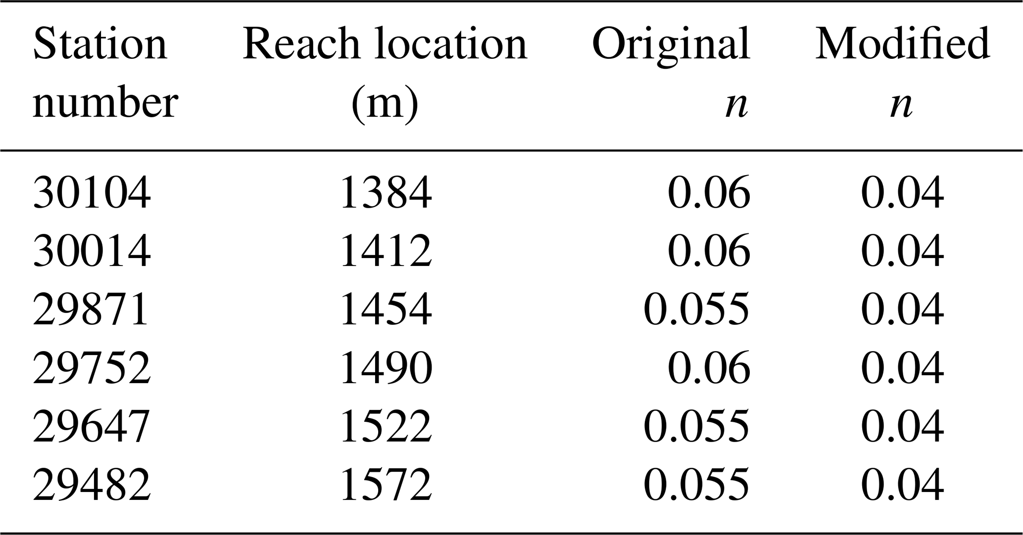
As discussed in Sect. 3, the stability of the SPRNT-RS simulations for Waller Creek was ensured by merging 36 computational elements in which the cross-section spacing was closer than 10 m. This minimum spacing cutoff was selected as being well below the median spacing of 28.6 m and mean spacing of 37.7 m and proved adequate for ensuring SPRNT-RS stability in the tested simulations. Unfortunately, stability of unsteady HEC-RAS required the further removal of three cross-section elements (shown in Fig. A1) and reducing Manning's n at six additional cross sections (listed in Table A1). Selecting these changes was a matter of art rather than science as we could not identify clear criteria for cross-section removal or Manning's n adjustments for HEC-RAS – other than that these locations appeared to be where instabilities appeared in unsteady HEC-RAS model runs. Although SPRNT-RS could run without these changes, for consistency in the model comparisons the geometry of the SPRNT-RS model was modified to exactly match the adjusted geometry required for the HEC-RAS model.

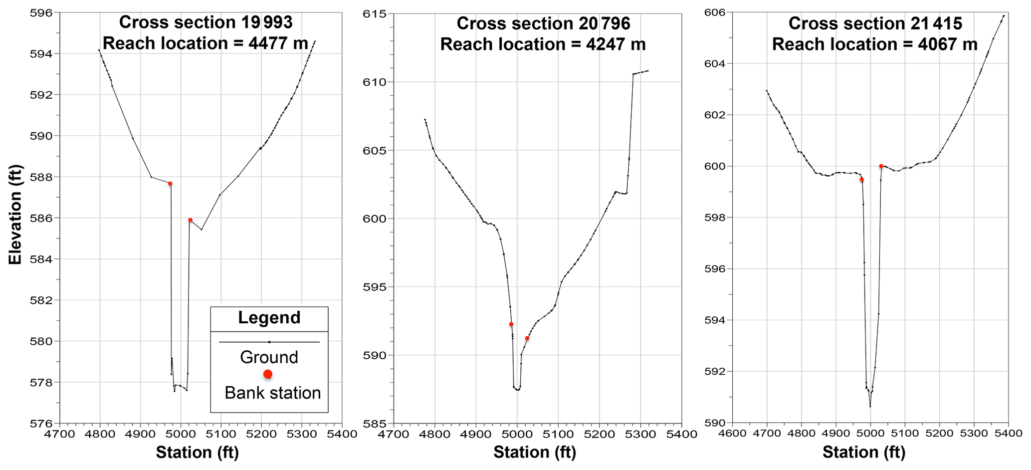
Figure A1 Cross sections removed from Waller Creek data set to provide numerical stability of unsteady HEC-RAS.

Table A1 Modified Manning's n for cross-section stations in Waller Creek data set to provide numerical stability of unsteady HEC-RAS.

Appendix B: Notation

A	cross-section area (m2)
g	gravitational acceleration (ms−2)
h0	water depth (m)
ha	associated water depth (m)
hR	reference height (m)
n	Gauckler–Manning–Strickler roughness (${\text{m}}^{-\mathrm{1}/\mathrm{3}}\text{s}$)
Pw	wetted perimeter (m)
Q	volumetric flow rate (m3s−1)
qℓ	flow rate per unit length through channel sides (m2 s−1)
S0	channel bottom slope
Sf	channel friction slope
SR	channel reference slope
SSW	channel sidewall slope
t	time (s)
W	channel width (m)
WB	channel bottom width ((m))
x	along-channel spatial coordinate
z0	channel bottom elevation (m)
zR	reference elevation (m)
α	bottom displacement coefficient
ϵ	second derivative of water surface elevation (m−1)
η	water surface elevation (m)
ρ	normalized difference between results
ζ	absolute mean normalized difference (AMND)