the Creative Commons Attribution 4.0 License.
the Creative Commons Attribution 4.0 License.
 | 21 Dec 2018
Developing a drought-monitoring index for the contiguous US using SMAP
Eric F. Wood
Since April 2015, NASA's Soil Moisture Active Passive (SMAP) mission has monitored near-surface soil moisture, mapping the globe (between 85.044∘ N/S) using an L-band (1.4 GHz) microwave radiometer in 2–3 days depending on location. Of particular interest to SMAP-based agricultural applications is a monitoring product that assesses the SMAP near-surface soil moisture in terms of probability percentiles for dry and wet conditions. However, the short SMAP record length poses a statistical challenge for meaningful assessment of its indices. This study presents initial insights about using SMAP for monitoring drought and pluvial regions with a first application over the contiguous United States (CONUS). SMAP soil moisture data from April 2015 to December 2017 at both near-surface (5 cm) SPL3SMP, or Level 3, at ∼36 km resolution, and root-zone SPL4SMAU, or Level 4, at ∼9 km resolution, were fitted to beta distributions and were used to construct probability distributions for warm (May–October) and cold (November–April) seasons. To assess the data adequacy and have confidence in using short-term SMAP for a drought index estimate, we analyzed individual grids by defining two filters and a combination of them, which could separate the 5815 grids covering CONUS into passed and failed grids. The two filters were (1) the Kolmogorov–Smirnov (KS) test for beta-fitted long-term and the short-term variable infiltration capacity (VIC) land surface model (LSM) with 95 % confidence and (2) good correlation (≥0.4) between beta-fitted VIC and beta-fitted SPL3SMP. To evaluate which filter is the best, we defined a mean distance (MD) metric, assuming a VIC index at 36 km resolution as the ground truth. For both warm and cold seasons, the union of the filters – which also gives the best coverage of the grids throughout CONUS – was chosen to be the most reliable filter. We visually compared our SMAP-based drought index maps with metrics such as the U.S. Drought Monitor (from D0–D4), 1-month Standard Precipitation Index (SPI) and near-surface VIC from Princeton University. The root-zone drought index maps were shown to be similar to those produced by the root-zone VIC, 3-month SPI, and the Gravity Recovery and Climate Experiment (GRACE). This study is a step forward towards building a national and international soil moisture monitoring system without which quantitative measures of drought and pluvial conditions will remain difficult to judge.
- Article
(13687 KB) - Full-text XML
- BibTeX
- EndNote


Drought is an extreme condition when water in one or a combination of water stores (e.g., river, lake, reservoir, snowpack, soil water or groundwater) or water fluxes (precipitation, evapotranspiration or runoff) drops below a defined condition for a prolonged period of time (AMS, 2012; Wilhite, 2000; Wilhite and Glantz, 1985). Such a water deficit evolves over weeks to months and can last for months and years. Drought's propagation is silent and often without warning until it impacts human lives and environmental activities (Tallaksen and Van Lanen, 2004). Drought conditions are related to water demand, so local water use plays a central role in defining conditions of scarcity and the resulting impacts. Wilhite and Glantz (1985) classified drought into meteorological, agricultural or hydrological, depending on whether the deficit is measured using precipitation, soil moisture or river discharge, respectively.
The reduced supply of precipitation (and subsequently soil moisture) for crops leads to an agricultural drought that impacts crop yield, inflicting enormous economic impacts on developed countries and the suffering of millions of people in less-developed regions of the world. In the US, since 1996, there has been at least one drought event per year except for the years 1997, 2001, 2004 and 2010, and each year drought cost between USD 1 billion and 14 billion in damages (in 2015 – adjusted dollars) (NOAA, 2018b). In California alone, the 2015 drought was estimated to cause USD 2–5 billion in damages to the agricultural sector (Howitt et al., 2015).
Although the impacts of drought are intimately linked to the vulnerability of a population to adverse conditions (UN/ISDR, 2007) and how society responds within the constraints of changing economies, the timely determination of the current level of agricultural drought aids the decision-making process in order to reduce its impacts. Scientifically based drought-monitoring tools and warning systems assist in the mitigation of the losses caused by droughts and the planing and management of water shortages that will accompany future droughts (Martinez-Fernandez et al., 2016). Such drought-monitoring tools are based on long-term observations of the hydrological variables such as precipitation, streamflow, soil moisture and groundwater.
Pluvial conditions are related to an abundance of precipitation and subsequently wet soil conditions that can adversely affect agriculture by waterlogging the fields or exacerbating flooding from additional rainfall. Thus, for monitoring extremes (either agricultural drought or pluvial conditions), realistic estimation of soil moisture at regional to continental scales is required. Soil moisture is the central source of information, since it reflects recent precipitation and antecedent soil conditions (Sheffield and Wood, 2011). In a sense, soil moisture captures the aggregate balance of all hydrological processes and represents available water, being a buffer between incoming precipitation and throughfall and evapotranspiration and drainage processes (Entekhabi et al., 1996). Unfortunately, soil moisture (and evapotranspiration) are among the least-observed components of the hydrological cycle, especially over large spatial and temporal scales (Reichle, 2017; Sheffield and Wood, 2011).
Many statistical measures or indices for extreme conditions have been developed in the US, particularly for drought conditions. This is due to the slow evolution of drought and its economic and social impact. Currently, no single drought index has been able to adequately capture the severity and intensity of drought and its impact on different groups of users (Heim, 2002). Heim (2002) gives an overview of the major 20th US drought indices. The most common ones are the standardized Precipitation Index (SPI), Palmer Drought Severity Index (PDSI), Standardized Runoff Index (SRI) and the U.S. Drought Monitor (DM or USDM).
The SPI is recognized by the World Meteorological Organization (WMO) as the standard index for quantifying and reporting meteorological drought. It is used to characterize drought on a range of timescales from 1 to 36 months. The raw precipitation is fit to an appropriate distribution function and is then transformed into a standardized normal distribution. The SPI index is expressed as the number of standard deviations by which the anomaly deviates from the long-term mean. On short timescales, the SPI is closely related to soil moisture, while at long timescales, it is related to groundwater. The advantages of the SPI include the following: it only relies on precipitation, it can characterize both drought and pluvial conditions, its computation over different timescales can be related to various water resource stores (such as soil moisture and groundwater), and it is more comparable across regions with different climates than the Palmer Severity Drought Index (PDSI). The key limitation of the SPI is the following: it is sensitive to the quantity of the data used. Usually, 30 years of monthly precipitation data are recommended for fitting the data. Additionally, the SPI is a meteorological tool that measures water supply but does not account for evapotranspiration. This limits its ability to capture the effect of increased temperatures (associated with climate change) on moisture demand and availability. Finally, the SPI does not consider the intensity of precipitation and how it impacts on runoff and streamflow. Overall, the SPI can provide information about anomalies in precipitation, so it needs to be used in combination with other information in order to be useful for agricultural drought assessment (NCAR, 2018).
The PDSI uses precipitation and an estimate of evaporation in conjunction with a water balance model to estimate relative soil dryness and potential evapotranspiration. The original formulation used only the temperature to estimate a potential evapotranspiration, but it is now recognized that an energy-based approach, such as the Penman–Monteith approach, is preferred (Mo and Chelliah, 2006; Sheffield et al., 2012). Since PDSI uses potential evapotranspiration and precedent (prior month) conditions, it takes into account the basic effect of global warming and is effective in determining long-term drought, especially over low and midlatitudes. Key limitations of the PDSI include that the PDSI is not as comparable across regions as the SPI and lacks the ability to handle winter-time conditions that include snowmelt and frozen precipitation, which makes its long-term monitoring problematic. Unlike SPI indices, the PDSI lacks multi-timescale features, making it difficult to correlate with specific water resources like runoff, snowpack and reservoir storage.
The SRI is based on the SPI and a model runoff. The strength of the SRI, as a runoff-based index, is that it can be used to forecast future runoff, and its predictability depends not only on climate outlooks, for which seasonal skill is generally low, but also on hydrologic initial conditions (e.g., spring snow state in the western US). The disadvantage of the SRI is similar to the disadvantage of using any modeled runoff; since modeled runoff cannot be verified everywhere, the runoff-based indices of the SRI reflect the customary uncertainties associated with model outputs (Shukla and Wood, 2008).
The USDM integrates several drought indices and professional input from all levels into a weekly operational drought-monitoring map product (Svoboda, 2000). The limitation of the USDM lies in its attempt to show drought at several temporal scales (from short-term drought to long-term drought) on one map product. Hence, the application of the DM is not for replacing any local or state information or subsequently declared drought emergencies or warnings but is rather for providing a general assessment of the current state of drought around the United States, its Pacific possessions, and Puerto Rico (Svoboda, 2000). Since the USDM relies on professional inputs from the field, it is difficult to have historical consistency (since the professionals change) or to provide forecasts.
Long-term and large-scale observations of soil moisture are scarce in the United States and elsewhere, so datasets produced by the North American Land Data Assimilation System (NLDAS) are valuable alternatives. Currently National Centers for Environmental Prediction (NCEP) offer an NLDAS drought monitor (NOAA, 2018a) based on four land surface models (LSMs): variable infiltration capacity (VIC), Noah, Mosaic and Sacramento. Sheffield et al. (2004) used simulations from the NLDAS VIC model forced with observed precipitation and near-surface meteorology to develop a drought index based on soil moisture. The approach Sheffield et al. (2004) took was to fit the VIC-simulated soil moisture to probability distributions, usually beta distributions, where the percentiles are translated to the index values that range from 0 to 1. Recent drought applications such as the VIC-based Princeton University drought and flood monitoring systems for Africa and Latin America (Sheffield et al., 2014) use the simulated soil moisture, which is mostly based on satellite precipitation (Princeton University Hydrology, 2013).
A major limitation of the indices discussed earlier, as well as of the LSM-based approaches, is a reliance on quality meteorological data. While precipitation is one of the best-observed variables, gauge observations are limited in many regions, especially in much of the developing world. Even when they are available, they are often not in near real time, preventing the computation of indices. This reveals one of the weaknesses of the above indices; their estimates rest on the availability and accuracy of the forcings, specifically precipitation (Reichle, 2017). In places such as the US, where the quality of the precipitation data is quite high, VIC quality is also relatively high (Pan et al., 2016). However, in regions with sparse networks or low accessibility, such as Africa, the VIC quality can be relatively low (Reichle, 2017). Additionally, intercomparison of the four NLDAS models showed that soil moisture differs considerably among models (Robock et al., 2000).
Heim (2002) summarizes four characteristics of a useful operational drought-monitoring system. These include the following: (1) the indices need to be available on a near-real-time basis, (2) the indices need to be monitored on a national scale, which will require the establishment of national networks for some variables, (3) complete and reliable historical data are needed over a common reference period to allow the conversion of the observations into a meaningful form (such as a percentile ranking), and (4) the data need to be adjusted to remove non-climatic influences (Friedman, 1957; Heim, 2002).
An alternative approach to using model-derived soil moisture for drought detection and prediction is satellite-derived soil moisture. There are currently four major satellite-based systems that provide soil moisture products at various spatial and temporal resolutions: MetOp with the advanced scatterometer (Brocca et al., 2010; Wagner et al., 2013), the Advanced Microwave Scanning Radiometer AMSR2 of the Japan Aerospace Exploration Agency (Parinussa et al., 2015; Wu et al., 2015) with the C- and X-band passive radiometers on the GCOM-W1 satellite that is a follow-on to the AMSR-E sensor, which failed on 4 October 2011 and was part of NASA's Earth Observing System, ESA's Soil Moisture Ocean Salinity (SMOS) L-band radiometer (Kerr et al., 2012, 2016; Pan et al., 2010), and NASA's Soil Moisture Active Passive (SMAP) L-band radiometer (Entekhabi et al., 2010). The radar on SMAP failed after 3 months, but soil moisture estimates based on the radiometer continue to be produced.
Of particular interest, especially for applications in parts of the globe with sparse in situ data, is to have an SMAP-based monitoring product that expresses soil moisture in terms of probability percentiles for dry (drought) or wet (pluvial) conditions (Entekhabi et al., 2010). This study presents insights and the potential of using SMAP for monitoring drought and pluvial regions with a first application over the contiguous United States (CONUS). We fit the soil moisture data from SMAP at both the level 3 5 cm passive radiometer retrievals (SPL3SMP) and the level 4 root-zone product that assimilates the surface SPL3SMP into the Catchment LSM (SPL4SMAU) to beta distributions, construct probability distributions for warm and cold seasons, and measure the reliability of our estimates. Producing soil moisture drought indices at two different soil depths allow for the monitoring of agricultural drought in different stages of development (NDMC, 2018a). This is important, firstly because grid analysis showed that values of a full column soil moisture index can be less, similar, or more than near-surface soil moisture index values. Secondly, depending on the plant development stage, the surface soil moisture or root-zone soil moisture drought index can be more useful in agricultural management. For example, surface soil moisture is important in the germination stage but is less important for managing irrigation or in estimating yields. Deficient topsoil moisture at planting may hinder germination, leading to low plant populations per hectare and a reduction of final yield (NDMC, 2018a). At the same time root-zone moisture at this early stage may not affect final yield, but as the growing season progresses, it becomes more important for plant water needs.
The rest of this paper as follows: the SMAP data are discussed in Sect. 2.1, including a determination of whether 1006 days are sufficient for estimating a drought index. Section 2.2 develops the indices by fitting beta distributions, with upper and lower bounds, to the time series and using the percentiles as the index. Section 2.3 develops a numerical analysis of the adequacy of the SMAP data. In Sect. 3, results of adequacy tests are discussed, and comparisons are made to the currently available drought indices. To help relate the percentiles to the U.S. Drought Monitor, which uses levels D0–D4 to indicate severity, the percentiles are mapped. We also extended our indices to pluvial conditions similar to the maps from the Gravity Recovery and Climate Experiment (GRACE) and Princeton University. Conclusions are brought forth in Sect. 4.
2.1 SMAP data
Since April 2015, NASA's SMAP mission has been monitoring near-surface soil moisture, mapping the globe (between 85.044∘ N and S) using an L-band (1.4 GHz) microwave radiometer in 2–3 days depending on location. The SMAP mission provides a set of operational global data products that include the following:
-
Level 3 (SPL3SMP) is a composite based on daily passive radiometer estimates of global land surface soil moisture (nominally 5 cm) that are resampled to a global, cylindrical 36 km Equal-Area Scalable Earth Grid, Version 2.0 (O'Neill et al., 2016). For this study, Version 4 of SPL3SMP is used, which is the release version from the very beginning of the launch of SMAP. The release number changes over time. The R16 version is the latest version released in June 2018. However, in all release versions of SMAP, including Version 4, regions with permanent snow and ice, frozen ground, excessive static or transient open water in the cell, excessive radio-frequency interference (RFI) in the sensor data, and heavy vegetation (vegetation water content >4.5 kg m−2) are masked out using a passive freeze–thaw retrieval based on the normalized polarization ratio (NPR). Given the 1000 km swath and 98.5 min orbit, the SPL3SMP retrievals are spatially and temporally discontinuous, with 2–3 day gaps depending on location.
-
Level 4 (SPL4SMAU) provides estimates of global surface and root-zone soil moisture by assimilating the SMAP L-band brightness temperature data (for which SPL3SMP is the gridded version) from descending and ascending half-orbit satellite passes, every 3 h from approximately 06:00 to 18:00 LST (Local Solar Time), into NASA's Catchment LSM (Reichle, 2017; Reichle et al., 2015). The SPL4SMAU data product is gridded using an Earth-fixed, global, cylindrical 9 km EASE-Grid 2.0 projection. The LSM component of the assimilation system is driven by a forcing data stream from the global atmospheric analysis system at the NASA Global Modeling and Assimilation Office (Rienecker et al., 2008). Additional corrections are applied using gauge- and satellite-based estimates of precipitation that are downscaled to the temporal and 9 km scale of the model forcing using the disaggregation methods described in Liu et al. (2011) and Reichle et al. (2011). The SPL4SMAU product provides global soil estimates for the surface (0–5 cm) and root zone (0–100 cm) and is an effort to provide continuous, daily information without discontinuous data restrictions due to gaps in the SPL3SMP soil moisture retrievals. Nonetheless, the only product that does not use ancillary meteorological data is the SPL3SMP soil moisture retrievals.
In this study, SPL3SMP products from the 06:00 LST retrievals and SPL4SMAU products from 06:00 LST retrievals are used in the analysis of the soil moisture drought index. Our SMAP data records are from 1 April 2015 to 31 December 2017, which is equivalent to 1006 days.
The approach selected here is somewhat similar to that of Sheffield et al. (2004), where the soil moisture time series are fit to a beta distribution (with upper and lower bounds), and the distribution percentiles are the index values. There are, however, differences in our approach to that of Sheffield et al. (2004). Firstly, the basis of the data used in Sheffield et al. (2004) was simulated soil moisture from VIC, while ours is remotely sensed data. Secondly, to calculate the bounds of beta distribution [a,b], Sheffield et al. (2004) used the first (last) 10 % of the sorted soil moisture values linearly related to the empirical cumulative distribution function. In our study, this approach did not yield useful results with the estimated limits for a (b) for SMAP and often did not cover the full range of observed values, preventing interpretation of the historical data. Our methodology for obtaining beta distribution parameters a and b are discussed in this section.
As mentioned in the introduction by Heim (2002), one of the conditions for an index approach is complete and reliable historical data needed over a common reference period to allow the conversion of the observations into a meaningful form. The short SMAP record length of 1006 days, from 1 April 2015 to 31 December 2017, provides a statistical challenge in estimating the drought and pluvial indices, and thus the reliability assessments related to these extreme conditions are necessary. Therefore, to assess the data adequacy, we used a 1979–2017 VIC LSM simulation over CONUS. The VIC runs were carried out at a 4 km spatial resolution, and for the SPL3SMP comparisons, averaged up to 36 km. Here we refer to it as VIC near surface (VIC-ns). The SPL4SMAU is at 9 km spatial resolution, so VIC data were aggregated from 4 km computing grids and averaged over three soil layers with varying total soil thickness. We refer to it as VIC root zone (or VIC-rz). A statistical comparison is made between fitting a beta distribution to the VIC soil moisture values using only days when SPL3SMP soil moisture retrievals are available and fitting it to the complete 1979–2017 VIC data record. The Kolmogorov–Smirnov (KS) statistical test was used to evaluate the consistency of the beta fitted data. We made the assumption that if grids passed the consistency test using VIC data – i.e., the distributions from the SMAP-period record and the complete record were deemed the same statistically – then the SMAP time series over that grid was sufficient for providing an index. More discussion of these results is given in Sect. 3.
Furthermore, we looked at the frequency distribution of soil moisture data at each grid. The data seemed to be dominated by low soil moisture in the summertime and high soil moisture in the wintertime. Therefore, to capture this inter-seasonal behavior in soil moisture, we divided the record into a warm season (April–September) and a cold season (October–March). Dividing the year into warm and cold seasons enabled us to track the soil moisture dynamics, and thus the probability distribution and index, seasonally. Ideally, we would have divided it into monthly data but there are insufficient observations.
For our study period, each grid has between 144 and 329 SPL3SMP soil moisture retrievals during the warm season and from 16 to 272 retrievals during the cold season. Figure 1 shows that the number of overpasses per grid is related to the latitude, with higher latitudes having a higher number of overpasses, and to the season, with fewer values retrieved during winter, especially in the western US, due to snow cover and frozen ground. For the LSPL4SMAU root zone, there are 457 records for the cold season and 549 records for the warm season for each grid.
2.2 Fitting the beta distribution to the SMAP time series
The beta distribution is a family of continuous distributions with two shape parameters (p and q). It generalizes to a bounded distribution on the interval of [a,b], where a and b usually take on the values of 0 and 1. The beta distribution is flexible enough to model a wide variety of shapes. In our study, we compared the beta distribution to several parametric distributions (including normal and Gumbel), but the beta distribution showed the best goodness of fit. Furthermore, given the bounded nature of the distribution, it is often used as the model of choice for modeling soil moisture time series (Sheffield et al., 2004). The general formula for the beta probability density function (pdf) is:
where p and q are shape parameters, and a and b are lower and upper bounds, respectively, of the distribution. In the case where a=0 and b=1, this becomes a standard beta distribution (NIST, 2013). B(p,q) is a beta constant computed with the formula
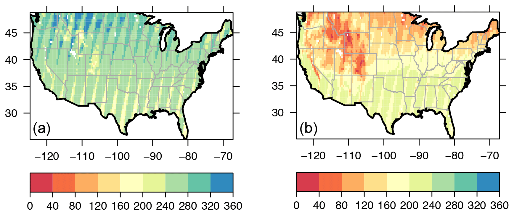
Figure 1Number of retrievals for each season. (a) Warm season (1 April–30 September); (b) cold season (1 October–31 March).

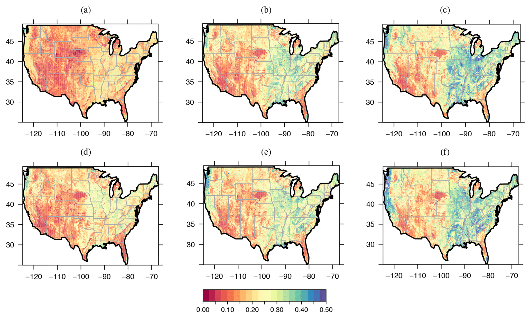
Figure 2(a–c) SMAP soil moisture values for the warm season during summer for SPL3SMP top 5 cm soil moisture (a) at the 20th percentile, (b) at the average soil moisture, and (c) at the 80th percentile; (d–f) same as the top row, but for the cold season. Total period is from 1 April 2015 to 31 December 2017. The soil moisture unit is m3 m−3.
A main challenge is to fit the four parameters of the beta distribution, given a set of empirical observations. Sheffield et al. (2004) used the method of moments to fit the beta distribution to historical soil moisture simulations from the VIC LSM. They computed the first three moments and minimized the difference between the distribution estimates and sample estimates, since they were over-constrained. We also used the standard method of moments to calculate the parameters p and q. But for each grid location, we fit the beta distribution to six sets of data related to the SPL3SMP product: (1) short warm season VIC, (2) short warm season SMAP (1 April–30 September for 2015, 2016 and 2017; 18 months), (3) long warm season VIC (1 April–30 September, 1979–2017; 129 months), (4) short cold season VIC, (5) short cold season SMAP (1 October–31 March, 2015–2016 and 1 October–31 December 2017; 15 months) and (6) long cold season VIC (1 October–31 March for 1979 and 2016 and 1 October–31 December for 2017; 126 months), using the first and second moments and , where p and q are parameters and its standard deviation is defined as
For the SPL4SMAU root-zone soil moisture product, the beta distribution was fit to the warm season and cold season using all 457 and 549 records, respectively.
Figure 2 shows the 20th percentile, average and 80th percentile soil moisture data in the warm season and cold season for the SPL3SMP 5 cm soil moisture product, and this is shown similarly in Fig. 3 for the SPL4SMAU root-zone product after data were fit to the beta distribution.
2.3 Data adequacy filters
An insufficient SMAP record length may result in unreliable index values. To be meaningful in using short SPL3SMP data for making confident predictions, we will analyze which grids have the highest certainty in our SMAP drought index. That is, we perform adequacy analysis and define filters that separate grids with high reliability in drought monitoring and prediction from ones where we do not expect our predictions to be as accurate. We first define two filters which can separate the 5815 grids covering CONUS into grids that passed and failed quality control. The two filters are as follows:
-
the KS test for beta-fitted long-term and short-term VIC with 95 % confidence;
-
good correlation (≥0.4) between beta-fitted VIC and beta-fitted SPL3SMP.
Below we expand upon these two filters and then show how we used them to numerically find the best SPL3SMP filter. We also investigate if combinations of the filters are superior to the individual filters taken alone.
2.3.1 Kolmogorov–Smirnov (KS) filter
The KS test is a well-known nonparametric statistical test that compares whether two samples are coming from the same continuous distribution. We used the KS test for each grid, comparing the modeled beta distribution of the long-term VIC with the modeled beta distribution of the short-term VIC, in both warm and cold seasons. This shows if the long-term and short-term distributions are statistically indistinguishable. If this strong condition is satisfied for a grid, then it is reasonable to assume, for that grid, that the short SMAP time series would be consistent with a hypothetical long SMAP time series. The null hypothesis – that the underlying beta distribution of short-term soil moisture data is the same as the underlying beta distribution of long-term soil moisture data for VIC – is rejected for values of the KS statistic D that exceed a critical value at the 95 % significance level: , where n is the number of observed variable (Lindgren, 1962).
2.3.2 Correlation filter
As mentioned earlier, one of the key assumptions of this paper is that if the beta distribution fit to the short-term VIC series is statistically consistent with beta fit to the long-term VIC time series, then we assume that the short-term beta-fitted SMAP series is consistent with the hypothetical long-term beta-fitted SMAP time series. This is possible because VIC modeled soil moisture is validated by ground measurements (Cai et al., 2017; Pan et al., 2016), and it is most plausible where the correlation between SPL3SMP and VIC is highest. Correlation maps are shown in Fig. 4 between SPL3SMP and the VIC-ns product for the warm season and cold season periods. This suggests another filter to use: require that the correlation of beta-fitted SPL3SMP and beta-fitted VIC soil moisture be relatively high. We examined the distribution of correlation values across all grids in order to pick the cutoff between high and low correlation. We chose the mean correlation, minus the standard deviation of correlation (across all grids), as a threshold. Thus grids whose correlation is close to average or better than the average pass the filter. For both the warm and cold seasons, this value was very close to 0.4, and as a result, we picked this as the common threshold.
2.3.3 Mean distance (MD)
To evaluate whether the KS-based filter, the correlation filter or a combination of both is best, we define a simple mean distance (MD) metric. Assuming that a VIC index at 36 km resolution is the ground truth, we can calculate a distance between VIC and SMAP. For every day that SMAP provided a retrieval, if SMAPi is the drought index percentile of grid i that passes the filter, and VICi is the VIC drought index percentile of the same grid, and in total ng grids on day d passed the filter, then the MDd is defined as the average of absolute distances between the SPL3SMP drought index percentiles and the VIC drought index percentiles. For the candidate date d and for a given filter,
In Eq. (4), VICi and SMAPi are VIC and SMAP drought index values for grid i, ng is the total number of grids that passed the filter, and MDd is the mean distance for date d.
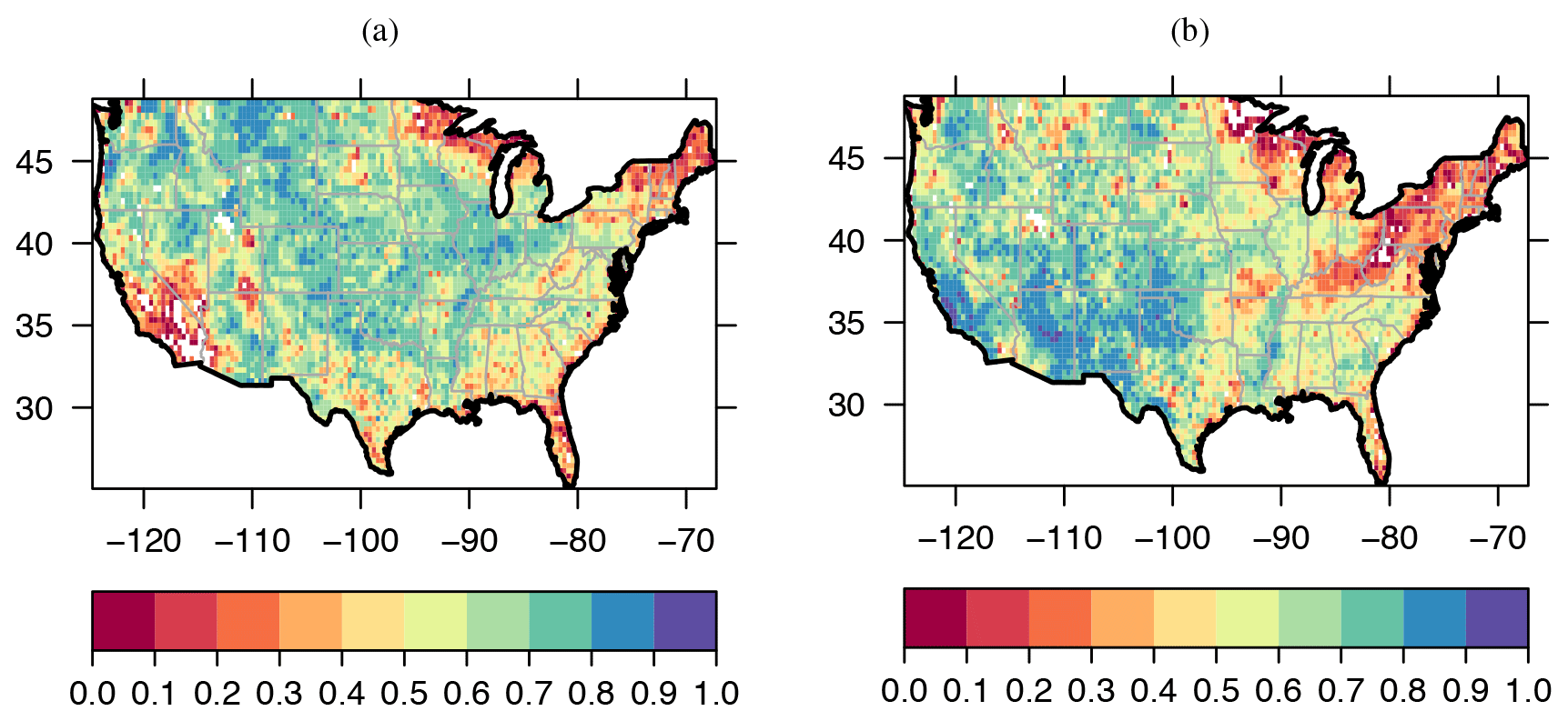
Figure 4(a) Correlations (R) between VIC and SMAP beta models for the warm season (average R=0.57) and (b) cold season (average R=0.56). White regions signify a negative correlation.
For each filter, the final pass and fail distance scores are calculated by averaging MDd values over the number of days, especially for both dry or wet seasons:
where nd is the total number of days for which the MDd value is available. While ng varies every day, since the number of overpasses varies every day, the value of nd was constant (549 for warm season and 457 for cold season). The MD value obtained from grids that failed a filter is called MDfail, and the MD value from grids that passed a filter is called MDpass. For each filter a difference (Diff) was computed by reducing the MDpass from the MDfail: .
2.3.4 Combination filters
In addition to the KS filter and the correlation filter, we investigate two filters defined by the following combination rules:
-
Intersection filter. A grid cell g passes the intersection filter if it passes both the KS filter and the correlation filter. Otherwise, it fails.
-
Union filter. A grid cell g passes the union filter if it passes either filter or both filters. Note that using the union filter gives the best coverage of the grids throughout CONUS, while the intersection filter has the strongest requirements for passing.
3.1 Data adequacy metrics
3.1.1 Correlation filter
Figure 4 shows that the average correlation for both warm and cold seasons is high and is around 0.6. During the warm season, the Central Valley and Southern California, Florida, the northeastern US, the north of Wisconsin, and Minnesota show poor correlation with VIC, at around 0.2. The extent of this poor correlation increases during the cold season for the northeastern US, Wisconsin and Minnesota. Snow season results in poor SMAP coverage during winter time in those areas. In addition, the low number of overpasses (presented in Fig. 1) during winter in the Northeast can play a role in the low amount of data and poor correlation during the cold season. Contrary to the warm season, southern California shows a high a correlation with VIC during the cold season, at around 0.9. We attribute this change from cold season to warm season in southern and southern-central California to the irrigation that SMAP picks up (Lawston et al., 2017) but VIC does not, since the version used here does not have water management effects. A land use and land cover map shows that about one-third of these areas are irrigated vegetation and another third are forests and woodlands (USGS, 2018). There are also as many as 2 million water wells in California that contribute to the irregularity of groundwater and affecting the soil moisture. They range from hand-dug, shallow wells to carefully designed large-production wells drilled to great depths (California Dept. of Water Resources, 2018). More data are needed before we can recognize further attributions to the low correlation between VIC and SMAP in that region. While systematic biases are not revealed in correlations, the temporal consistency among the time series is captured.
3.1.2 KS filter
Figure 5 shows which grids passed the 95 % KS test; there, we have confidence that the SMAP drought (pluvial) indices provide reliable risk levels given the current period of record. The warm season shows 11 % more grids passing the adequacy test than the cold season. Note that as the record length gets extended, the above analysis needs to be repeated to see if the adequacy changes.
In the warm season, the majority of the grids whose underlying short-term and long-term beta distribution were different were in the western US. The low warm season correspondence in the Pacific Northwest (PNW) region is particularly apparent. The PNW region is covered by dense forests, mountain and heavily regulated agricultural lands by irrigation. This contributes to the fact that most grids in PNW do not pass the KS filter. A pattern of low correspondence over the major mountain areas (e.g., the Rocky Mountains, Sierra and Cascades) is also apparent, given the coarse SMAP brightness temperature (Tb) footprint and dense vegetation.
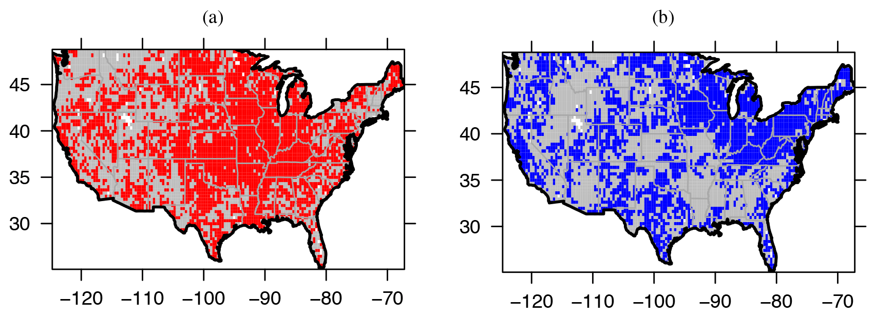
Figure 5(a) Grids in red show areas whose short-term VIC in warm season data has the same underlying beta distribution as the long-term VIC in warm season data (n=3560 or 68 % of grids are red); (b) the same as panel (a), but for cold season period shown in blue (n=2927 or 57 % of grids). Gray areas are grids where the short-term VIC does not have the same beta distribution as their long-term VIC.
3.1.3 Combined filters
Figure 6 represents the results of correlation filter and KS filter together for both warm (panel a) and cold (panel b) seasons over all 5815 grids. We use these filters (passed and failed grids) on a daily basis for MDd measures, though the value changes every day, depending on the number of overpasses for that date. Table 1 summarizes how many grids pass or fail each filter.
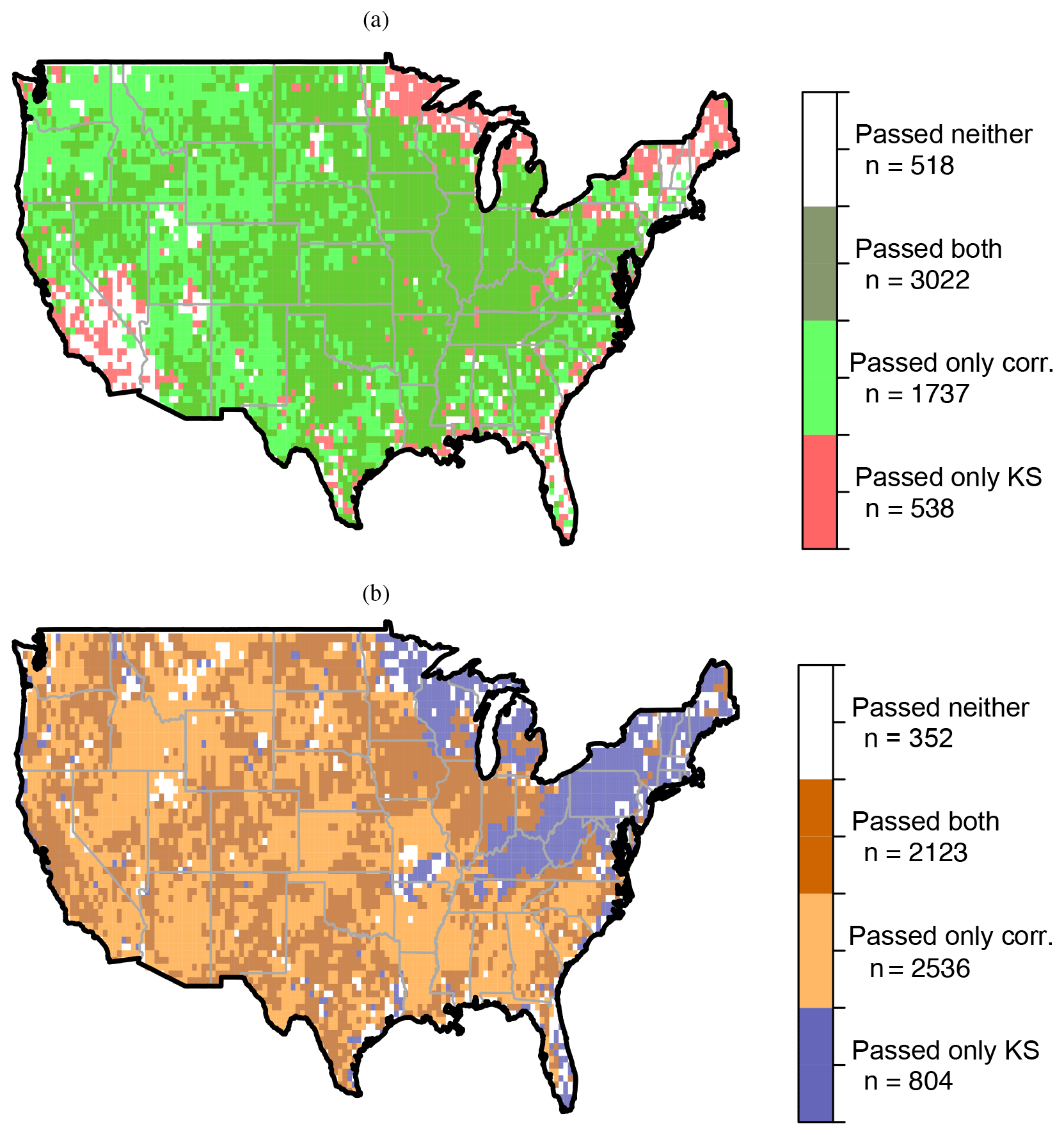
Figure 6(a) Warm season grids that pass the correlation filter and/or the KS filter. Dark green grids include grids that pass intersection filters. (b) Cold season grids that pass the correlation filter and/or the KS filter. Dark orange grids include grids that pass intersection filters. In both figures, white grids show the grids that pass neither filter and will be cross-hatched in index maps.
3.2 Evaluation of results under different filters
For each filter, the values of MDd were averaged to calculate MDfail and MDpass for the whole CONUS over the 549 days of the warm season and 457 days of the cold season. The summary result of all four tests is shown in Tables 2 and 3. To test if having a filter is better than having no filter, for each season, we performed a two-sided null hypothesis. The tests used 95 % confidence limits between the MD of all grids – which was 22.7 in the warm season and 22.6 in the cold season – versus the MD of only passed grids. The results showed that all four filters are significantly different than the MD of the whole CONUS. Thus, regardless of the type of the filter, having some sort of filter is better than having no filter.
Table 1Number of grids, out of total 5815, that fail and pass the quality control for each filter.
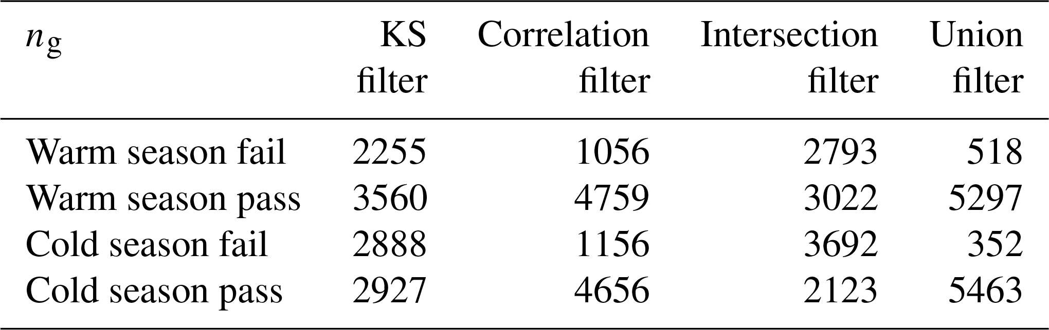
Note: per day, the ng numbers are less because of SMAP overpass missing grids.
In the warm season, the KS filter did better (i.e., larger Diff values or better skill in separating high- and low-performance grids) than the correlation filter for only 115 days out of 546 days, mostly in April. For almost half of the dates (260 days out of 546), the union filter did better than the correlation filter. This outperforming of the union filter occurs evenly throughout the warm season.
In the cold season, for only 48 days out of 457 days, the KS filter did better than the correlation filter, and for 198 days, the union filter did better than the correlation filter. These results suggest that for the cold season, the correlation filter is providing the most effective filter. However, if we only accept the grids that pass the correlation filter, we lose 804 grids. This area involved almost all of the northeastern coast and central East Coast as well as northern Wisconsin and northeastern Minnesota. However this is not a concerning problem for drought, since for most of the cold season these areas are covered by snow. We still decided to generate a cold season filter by including the KS filter with the correlation filter, thus we used the union filter for the cold season.
Table 2Mean distance (MD) of four tests averaged over 549 days of warm season. Diff is the difference between the first and second row.
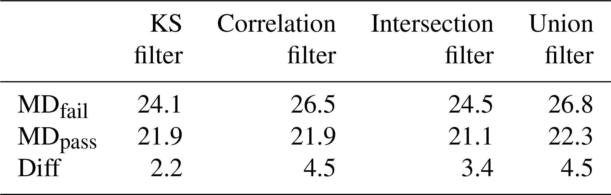
Table 3Mean distance (MD) of four tests averaged over 457 days of cold season. Diff is the difference between the first and second row.
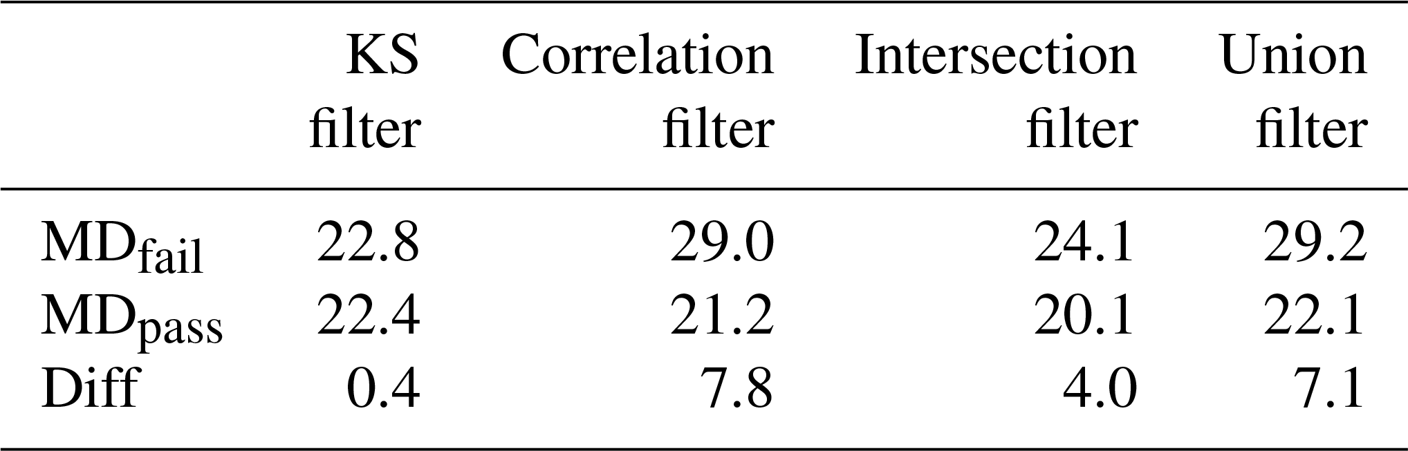
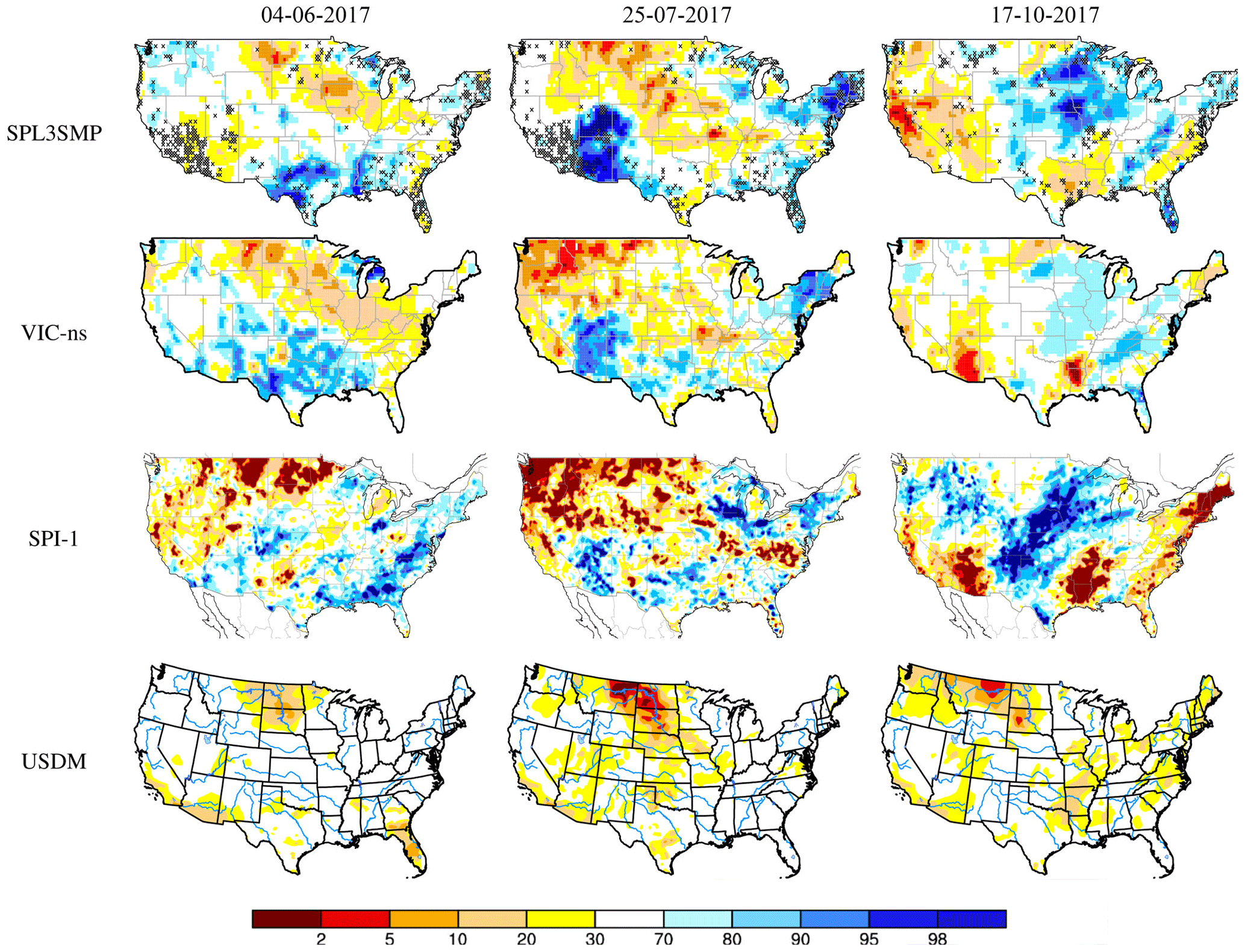
Figure 7Comparison between SPL3SMP index map and VIC-ns, SPI-1 and USDM in 2017. The black x symbols in the SPL3SMP maps are the grids that passed neither filter and were shown as white grids in Fig. 6. For USDM, drought levels from 30 to 100 are shown in white.
Three considerations for doing so are the following:
-
The Diff values. The correlation-filter Diff value and union-filter Diff value during the cold season are similar and close.
-
The nature of our tests. It is not that surprising that the correlation filter has a higher Diff than that of the union filter. The MD metric measures how the SMAP index resembles the VIC index. Thus, we find that the most important predictor is that the SMAP values should be correlated with the VIC values.
-
Optimum coverage. Although the cold season East Coast drought index is not a matter of concern for this study, cold season soil moisture variability can affect warm season soil moisture and consequently agricultural drought. The goal is to create a filter that does not lose important information while providing the best knowledge of soil moisture data.
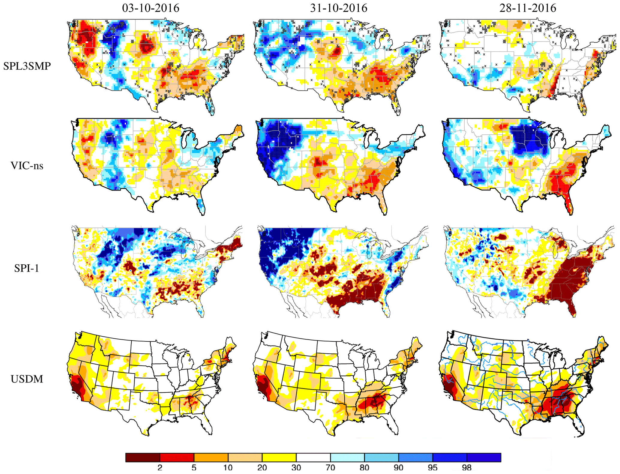
Figure 8Comparison between SPL3SMP index map and VIC-ns, SPI-1 and USDM in 2016. The black x symbols in the SPL3SMP maps are the grids that passed neither filter and were shown as white grids in Fig. 6. For USDM, drought levels from 30 to 100 are shown in white.
During the warm season, most of the grids that failed the test were in southern California and southern Nevada, in the Northeast (New Hampshire, Massachusetts, and Connecticut), and in the Southeast along the eastern coast of Florida. These are attributed to both the lack of correlation between SMAP and VIC and high variability between short-term and long-term soil moisture. These areas show non-stationarity in soil moisture, meaning that soil moisture distribution is subject to change over time, either due to climate or human interventions. During the cold season, most of the areas are covered using the union filter. However, as discussed, we use this filter with caution, knowing that at least according to our numerical analysis, the correlation filter did better than the union filter. The Great Lakes region, Minnesota, and the Mid-Atlantic region do not show a high correlation between VIC and SMAP in the cold season. Snow, heavy canopy and land development cause SMAP retrievals to have errors. In addition, this region does not have a good coverage of soil moisture and has a smaller number of retrievals per grid (Fig. 1). However, the KS filter complements the map by showing that the long-term and short-term VIC during cold season stays pretty stationary over time. This means that the soil moisture in this area has been less subject to change during cold season at least for the past 40 years.
This information can be used to inform an interpretation of SMAP soil moisture percentiles maps based on <10 years of data, as presented in Figs. 7 and 8 for a selection of soil moisture drought and flood indices. The grids that fail both KS and correlation tests (white grids in Fig. 6) will be flagged and are where we have the highest uncertainty of the quality of the data. This includes about 500 grids in the warm season and about 350 grids in the cold season over the CONUS.
3.3 Comparison of the drought indices
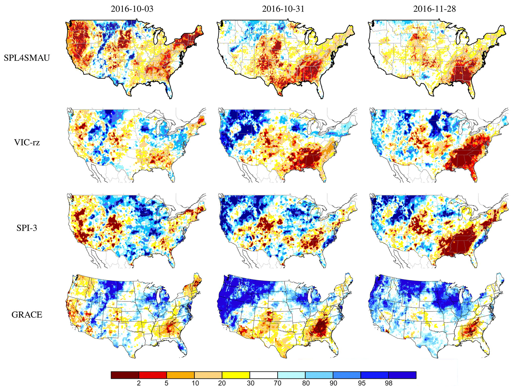
In Figs. 7 to 10, several indices are compared to the SMAP-based drought index. For the surface soil moisture index based on SPL3SMP, we provide a 3-day composite SMAP index to offer more continuous coverage. The union filter is applied to omit the grids that do not have reliable estimates. Our index SPL3SMP index maps are compared with the 1-month SPI (SPI-1) index, a VIC-ns index and the USDM. For SMAP soil moisture index based on the SPL4SMAU, comparisons are made with a 3-month SPI (SPI-3) index and a GRACE satellite product. All the products except for GRACE were described in Sect. 1. GRACE is NASA's satellite system that detects small changes in the Earth's gravity field caused by the redistribution of water on and beneath the land surface. Combined with the Catchment LSM using an ensemble Kalman smoother for data assimilation (Zaitchik et al., 2008), GRACE maps root-zone soil moisture and groundwater transformed into percentiles (NDMC, 2018b).
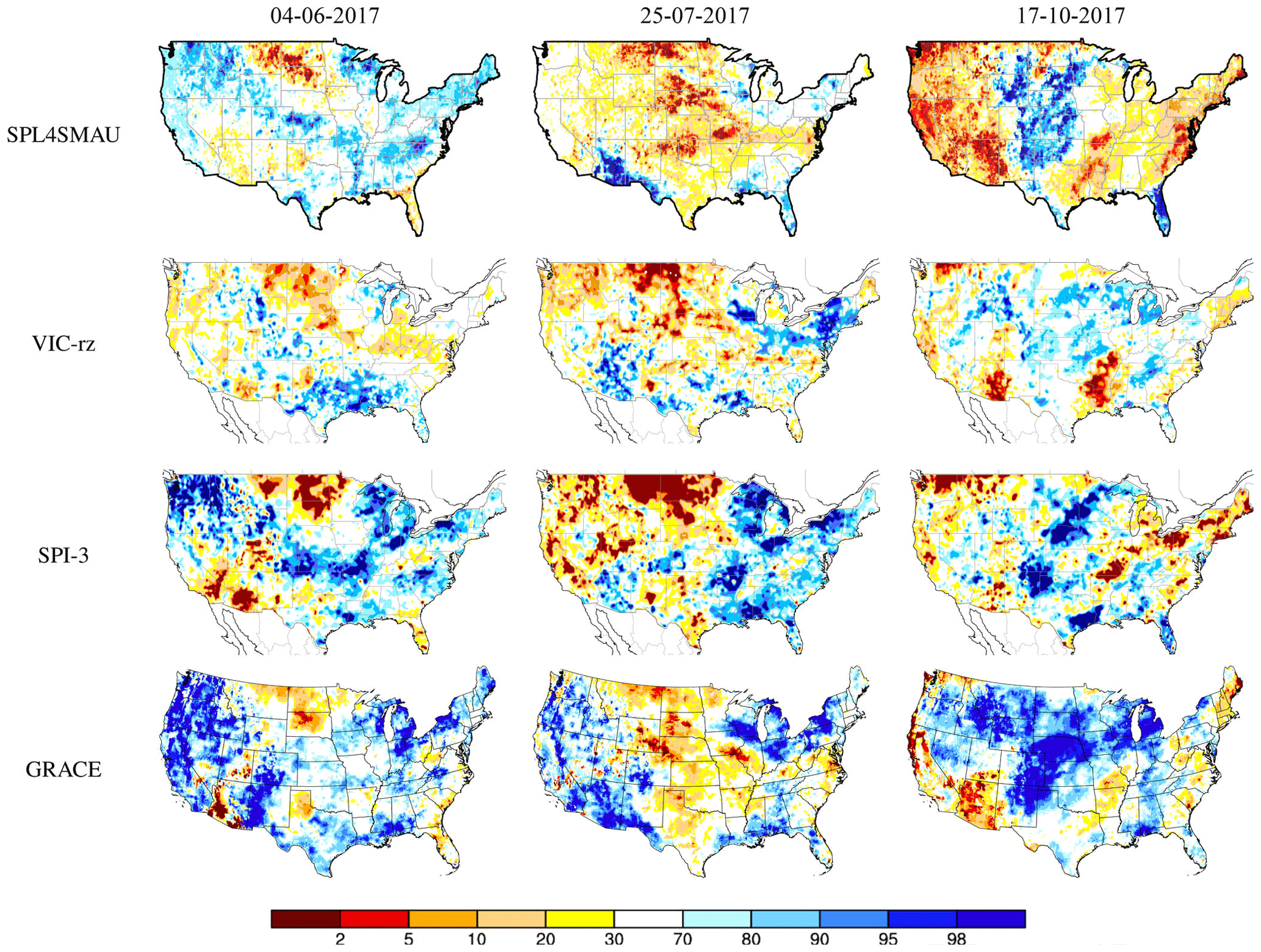
Figures 7 and 9 show drought during the period from 4 June through 17 October 2017, for both the near surface and root zone. In this period, there was one agricultural drought event in Montana and North and South Dakota, with losses exceeding USD 1 billion across the United States (NOAA, 2018b). The plains of eastern Montana experienced exceptional drought from July to October 2017, and in late October, drought started to end. The peak of the drought was in July 2017 when 20 % of Montana was in severe drought and 23 % of it was in moderate drought. Concurrently, 40 % of North Dakota was in extreme drought, while 70 % of the state was under some level of drought; similarly, 68 % of South Dakota was under severe drought (NOAA, 2018b). Both SPL3SMP and SPL4SMAU index maps seem to catch this drought event, although the event was more pronounced in the root zone than the surface. The maps of these two figures are also in general agreement. It is important to clarify that for 2017 period, the GRACE sensor was failing, and the resulting water storage observations were unreliable. Therefore, the last GRACE gravity field retrieval processing only goes through June 2017. Therefore, GRACE National Drought Mitigation Center (NDMC) results associated with Fig. 9 are not consistent with other products and likely do not reflect actual GRACE observations for 2017.
In Figs. 8 and 10, drought during the period of 3 October to 8 November 2016 is shown for both near the surface and the root zone. In 2016, there were three drought events in the western, northeastern and southeastern parts of the US, which are captured by both SPL3SMP and SPL4SMAU index maps. The drought had mostly been alleviated in northern California by near-normal precipitation during the 2015–2016 winter and above normal precipitation in fall 2016. The extent that the drought persisted in Southern California after this period it is reflected in total column soil moisture rather than near-surface soil moisture (Fig. 9).
There is a high correspondence among the drought maps, particularly in the development of the drought in the southeastern US during October and November 2016. Due to heavy rainfall along the Mississippi River in November, the drought migrated eastwards. Also, by November 2016 the drought in Southern California was alleviated, which is picked up by SPL3SMP, SPL4SMAU, VIC-ns and VIC-rz, SP-1 and 3, GRACE, and to a much lesser extent, by the USDM that showed an increasing area under drought on 28 November compared to SPL3SMP, SPL4SMAU, GRACE, or VIC-ns and VIC-rz. Additionally, for the maps that also include wetness (all except USDM), there is a high correspondence of pluvial regions (see Fig. 7).
Most of the grids where we do not have confidence in the accuracy of predictions are in Southern California and Nevada during the warm season (e.g., SPL3SMP index map on 4 June and 25 July 2017; Fig. 7). In fact, there is a visible discrepancy between SPL3SMP and VIC-ns index maps during that period in Southern California. We believe that this is due to a lack of correlation between SPL3SMP and VIC-ns in that area, since VIC does not model regulation. Human interference and the use of groundwater wells during the warm season can play a major part in what VIC models and SMAP see. For that reason, we think SMAP's metrics in the area are more accurate than those from VIC-ns.
The drought index described in this study provides a reliable estimate of the state of drought on a daily basis for the CONUS, using SMAP. We fitted beta distributions to the SMAP data and used correlation, KS, and a combination of those two filters to numerically assess the adequacy of the short-term SMAP data for each grid cell. The areas that passed neither the KS nor correlation tests were flagged in the final SMAP drought index. These areas are grids where we have less confidence in reliable drought index estimates; they are non-stationary, and thus their soil moisture has been changing over the past 40 years. The flagged grids can be seen as an adjustment to the model to remove non-climatic influences or water management practices, although more in-depth research is needed to confirm such changes. Given the limited scope of the data, the results should be considered a demonstration of the reliability and usefulness of SMAP for a drought-monitoring product and for implementation into an operational drought-monitoring tool.
Besides drought, SMAP can also identify regions of anomalously wet conditions that can be of great use to water and agricultural managers. Wet indices can indicate potential flood-prone conditions and regions can therefore be put on flood alerts if additional heavy rain occurs. Also, wet conditions can impact farm management, especially in the spring when sowing takes place or during the harvesting period.
Through comparing SMAP-based index maps for drought and wet conditions with other index products, we see a high similarity. Although there can be some errors at different levels, the overall evaluation reveals that SMAP-based drought products can be a viable alternative for drought monitoring in the US. This is advantageous, since SMAP is generated at a daily resolution with almost complete coverage every 3 days. This enables an observation of the effect of fluctuations in other hydrological variables, such as precipitation. In comparison, USDM, GRACE and the SPI have a low temporal resolution, which makes it difficult to study the shorter-term impacts from the other variables on soil moisture.
Both near-surface and root-zone soil moisture drought products can provide important information about the availability of soil moisture at the stage where plants develop in order to cultivate the optimum harvest. Future applications of this study can couple plant growth models with near-surface and root-zone soil moisture drought index products (NDMC, 2018a).
The soil moisture data are a culmination of all hydrological processes and represent available water from incoming precipitation and throughfall to evapotranspiration and drainage processes. The SMAP satellite provides global observations of soil moisture of unprecedented quality. Because SMAP monitors soil moisture directly and provides critical information for drought early warning, it is important that the future developments focus on drought assessment using SMAP in underrepresented parts of the world. Thus the results here provide significant support for a global SMAP drought and pluvial conditions monitoring system. Since SMAP data can be retrieved and maps can be generated in near-real time, it is very promising that a SMAP drought index product can be implemented operationally.
The SMAP-based drought index product at the daily resolution for CONUS is available at http://hydrology.princeton.edu/~sadri/nasasmap/index.html (last access: 17 December 2018). The USDM and GRACE maps were provided by the National Drought Mitigation Center at the University of Nebraska–Lincoln and were downloaded from their websites at http://droughtmonitor.unl.edu (last access: 17 December 2018) and at http://nasagrace.unl.edu (last access: 17 December 2018), respectively. The VIC data were provided by Ming Pan from Princeton University's Terrestrial Hydrology Group.
SS carried out the drought index development, developed the confidence analysis and online near-real-time website, and drafted the paper. MP prepared the VIC and SMAP soil moisture data as well as SPI drought index maps. EFW conceived of the study, supervised the project and helped to draft the paper. All authors read and approved the final paper.
The authors declare that they have no conflict of interest.
This work was supported by NASA grant CNV1003235. This paper benefited
greatly from the reviewers' comments. We thank them for their time and
support.
Edited by: Nunzio Romano
Reviewed by: John Kimball and two anonymous referees
AMS: Drought, available at: http://glossary.ametsoc.org/wiki/Drought (last access: 30 April 2018), 2012. a
Brocca, L., Hasenauer, S., Lacava, T., Melone, F., Moramarco, T., Wagner, W., Dorigo, W., Matgen, P., Martinez-Fernandez, J., Llorens, P., Latron, J., Martin, C., and Bittelli, M.: Soil moisture estimation through ASCAT and AMSR-E sensors: An intercomparison and validation study across Europe, Remote Sens. Environ., 115, 3390–3408, https://doi.org/10.1016/j.rse.2011.08.003, 2010. a
Cai, X., Pan, M., Chaney, N. W., Colliander, A., Misra, S., Cosh, M. H., Crow, W. T., Jackson, T. J., and Wood, E. F.: Validation of SMAP soil moisture for the SMAPVEX15 field campaign using a hyper-resolution model, Water Resour. Res., 53, 3013–3028, 2017. a
California Dept. of Water Resources: Wells, available at: https://water.ca.gov/Programs/Groundwater-Management/Wells, last access: 25 April 2018. a
Entekhabi, D., Rodriguez-Iturbe, I., and Castelli, F.: Mutual interaction of soil moisture state and atmospheric processes, J. Hydrol., 184, 3–17, 1996. a
Entekhabi, D., Njoku, E. G., O'Neill, P. E., Kellogg, K. H., Crow, W. T., Edelstein, W. N., Entin, J. K., Goodman, S. D., Jackson, T. J., Johnson, J., Kimball, J., Piepmeier, J. R., Koster, R. D., Martin, N., McDonald, K. C., Moghaddam, M., Moran, S., Reichle, R., Shi, J. C., Spencer, M. W., Thurman, S. W., Tsang, L., and Van Zyl, J.: The Soil Moisture Active Passive (SMAP) Mission Proc., IEEE, 98, 704–716, https://doi.org/10.1109/JPROC.2010.2043918, 2010. a, b
Friedman, D. G.: The prediction of long-continuing drought in south and southwest Texas, Occasional Papers in Meteorology, p. 182, the Travelers Weather Research Center, Hartford, CT, USA, 1957. a
Heim Jr., R. R.: A review of twentieth century drought indices used in the United States, B. Am. Meteorol. Soc., 83, 1149–1165, 2002. a, b, c, d, e
Howitt, R. E., Medellin-Azuara, J., MacEwan, D., Lund, J. R., and Daniel, A.: Economic Impact of the 2015 Drought on Farm Revenue and Employment Sumner, Agricultural and Resource Update, Giannini Foundation of Agricultural Economics, University of California, Davis, USA, 2015. a
Kerr, Y. H., Waldteufel, P., Richaume, P., Wigneron, J. P., Ferrazzoli, P., Mahmoodi, A., Al Bitar, A., Cabot, F., Gruhier, C., Juglea, S. E., Leroux, D., Mialon, A., and Delwart, S.: The SMOS Soil Moisture Retrieval Algorithm, IEEE T. Geosci. Remote, 50, 1384–1403, https://doi.org/10.1109/TGRS.2012.2184548, 2012. a
Kerr, Y. H., Al-Yaari, A., Rodriguez-Fernandez, N., Parrens, M., Molero, B., Leroux, D., Bircher, S., Mahmoodi, A., Mialon, A., Richaume, P., Delwart, S., Pellarin, A. A. B. T., Bindlish, R., Rudiger, T. J. C., Waldteufel, P., Mecklenburg, S., and Wigneron, J.: Overview of SMOS performance in terms of global soil moisture monitoring after six years in operation, Remote Sens. Environ., 180, 40–63, https://doi.org/10.1016/j.rse.2016.02.042, 2016. a
Lawston, P. M., Santanello Jr., J. A., and Kumar, S. V.: Irrigation Signals Detected From SMAP Soil Moisture Retrievals, Geophys. Res. Lett., 44, 11860–11867, 2017. a
Lindgren, B.: Statistical Theory, Mac-millan, New York, USA, 1962. a
Liu, Q., Reichle, R. H., Bindlish, R., Cosh, M. H., Crow, W. T., de Jeu, R., Lannoy, G. J. M. D., Huffman, G. J., and Jackson, T. J.: The contributions of precipitation and soil moisture observations to the skill of soil moisture estimates in a land data assimilation system, J. Hydrometeorol., 12, 750–765, 2011. a
Martinez-Fernandez, J., Gonzalez-Zamora, A., Sanchez, N., and A Gumuzzio, .: Satellite soil moisture for agricultural drought monitoring: Assessment of the SMOS derived Soil Water Deficit Index (vol. 177, pg. 277, 2016), Remote Sens. Environ., 183, 368–368, 2016. a
Mo, K. C. and Chelliah, M.: The modified Palmer Drought Severity Index based on the NCEP North American Regional Reanalysis, J. Appl. Meteor. Climatol., 45, 1362–1375, 2006. a
NCAR: The Climate Data Guide: Standardized Precipitation Index (SPI), available at: https://climatedataguide.ucar.edu/climate-data/standardized-precipitation-index-spi, last access: 2 April 2018. a
NDMC: Types of Drought, National Drought Monitoring Center, available at: https://drought.unl.edu/Education/DroughtIn-depth/TypesofDrought.aspx, last access: 17 December 2018a. a, b, c
NDMC: Groundwater and Soil Moisture Conditions from GRACE Data Assimilation, the National Drought Mitigation Center University of Nebraska-Lincoln, available at: http://nasagrace.unl.edu/Archive.aspx, last access: 17 December 2018b. a
NIST: Beta Distribution, available at: http://www.itl.nist.gov/div898/handbook/eda/section3/eda366h.htm (last access: 2 April 2018), 2013. a
NOAA: NLDAS Drought Monitor Soil Moisture, available at: http://www.emc.ncep.noaa.gov/mmb/nldas/drought/, last access: 5 February 2018a. a
NOAA: U.S. Billion-Dollar Weather and Climate Disasters, national Centers for Environmental Information (NCEI), available at: https://www.ncdc.noaa.gov/billions, last access: 4 October 2018b. a, b, c
O'Neill, P., Chan, S., Njoku, E. G., Jackson, T., and Bindlish, R.: SMAP L2 Radiometer Half-Orbit 36 km EASE-Grid Soil Moisture, Distributed Active Archive Center Version 4, NASA National Snow and Ice Data Center, Boulder, Colo., USA, https://doi.org/10.5067/XPJTJT812XFY, 2016. a
Pan, M., Li, H., and Wood, E.: Assessing the skill of satellite-based precipitation estimates in hydrologic applications, Water Resour. Res., 46, W09535, https://doi.org/10.1029/2009WR008290, 2010. a
Pan, M., Cai, X., Chaney, N. W., Entekhabi, D., and Wood, E. F.: An initial assessment of SMAP soil moisture retrievals using high-resolution model simulations and in situ observations, Geophys. Res. Lett., 43, 9662–9668, 2016. a, b
Parinussa, R. M., Holmes, T. R. H., Wanders, N., Dorigo, W. A., and de Jeu, R. A. M.: A Preliminary Study toward Consistent Soil Moisture from AMSR2, J. Hydromet., 16, 932–947, https://doi.org/10.1175/JHM-D-13-0200.1, 2015. a
Princeton University Hydrology: http://stream.princeton.edu/CONUSFDM/WEBPAGE/interface.php?locale=en (last access: 15 December 2018), 2013. a
Reichle, R. H.: Assessment of the SMAP Level-4 Surface and Root-Zone Soil Moisture Product Using In Situ Measurements, J. Hydrometeorol., 18, 2621–2645, 2017. a, b, c, d
Reichle, R. H., Koster, R. D., Lannoy, G. J. M. D., Forman, B. A., Liu, Q., Mahanama, S. P. P., and Toure, A.: Assessment and enhancement of MERRA land surface hydrology estimates, J. Climate, 24, 6322–6338, 2011. a
Reichle, R. H., Lucchesi, R., Ardizzone, J. V., Kim, G., Smith, E. B., and Weiss, B. H.: Soil Moisture Active Passive (SMAP) Mission Level 4 Surface and Root Zone Soil Moisture (L4SM) Product Specification Document, Tech. Rep. 10 (Version 1.4), NASA Goddard Space Flight Center, Greenbelt, MD, USA, 2015. a
Rienecker, M., Suarez, M. J., Todling, R., Bacmeister, J., Takacs, L., Liu, H.-C., Gu, W., Sienkiewicz, M., Koster, R. D., Gelaro, R., Stajner, I., and Nielsen, J. E.: The GEOS-5 Data Assimilation System – Documentation of Versions 5.0.1, 5.1.0, and 5.2.0., NASA Technical Report Series on Global Modeling and Data Assimilation NASA/TM-2008-104606, NASA, vol. 28, 101 pp., 2008. a
Robock, A., Vinnikov, K., Srinivasa, G., Entin, J., Hollinger, S., Speranskaya, N., Liu, S., and Namkhai, A.: The Global Soil Moisture Data Bank, B. Am. Meteorol. Soc., 81, 1281–1299, 2000. a
Sheffield, J. and Wood, E. F.: Drought: Past Problems and Future Scenarios, 978-1-84971-082-4, EarthScan, London, UK, 2011. a, b
Sheffield, J., Goteti, G., Wen, F., and Wood, E. F.: A simulated soil moisture based drought analysis for the United States, J. Geophys. Res., 109, D24108, https://doi.org/10.1029/2004JD005182, 2004. a, b, c, d, e, f, g, h
Sheffield, J., Livneh, B., and Wood, E. F.: Representation of terrestrial hydrology and large scale drought of the Continental U.S. from the North American Regional Reanalysis, J. Hydrometeor., 13, 856–876, https://doi.org/10.1175/JHM-D-11-065.1, 2012. a
Sheffield, J., Wood, E. F., Chaney, N., Guan, K., Sadri, S., Yuan, X., Olang, L., Amani, A., Ali, A., and Demuth, S.: A Drought Monitoring and Forecasting System for Sub-Sahara African Water Resources and Food Security, B. Am. Meteorol. Soc., 95, 861–882, 2014. a
Shukla, S. and Wood, A. W.: Use of a standardized runoff index for characterizing hydrologic drought, Geophys. Res. Lett., 35, 1–7, 2008. a
Svoboda, M.: An introduction to the Drought Monitor, Drought Network News, 12, 15–20, 2000. a, b
Tallaksen, T. and Van Lanen, H. A.: Hydrological Drought, Processes and Estimation Methods for Streamflow and Groundwater, vol. 48, Elsevier Science, Amsterdam, the Netherlands, 2004. a
UN/ISDR: Drought Risk Reduction Framework and Practices: Contributing to the Implementation of the Hyogo Framework for Action. United Nations Secretariat of the International Strategy for Disaster Reduction (UN/ISDR), Tech. Rep. 98+vi pp., United Nations Secretariat of the International Strategy for Disaster Reduction (UN/ISDR), Geneva, Switzerland, 2007. a
USGS: National Gap Analysis Program, Land Cover Data Viewer,, available at: https://goo.gl/rntijg, last access: 30 April 2018. a
Wagner, W., Hahn, S., Kidd, R., Melzer, T., Bartalis, Z., Hasenauer, S., Figa-Saldaña, J., de Rosnay, P., Jann, A., Schneider, S., Komma, J., Kubu, G., Brugger, K., Aubrecht, C., Züger, J., Gangkofner, U., Kienberger, S., Brocca, L., Wang, Y., Blöschl, G., Eitzinger, J., and Steinnocher, K.: The ASCAT Soil Moisture Product: A Review of its Specifications, Validation Results, and Emerging Applications, Meteorol. Z., 22, 5–33, https://doi.org/10.1127/0941-2948/2013/0399, 2013. a
Wilhite, D. A.: Drought as a Natural Hazard: Concepts and Definitions, chap. 1, vol. I, National Drought Mitigation Center at Digital Commons at University of Nebraska, Lincoln, Routledge, London, UK, 2000. a
Wilhite, D. A. and Glantz, M. H.: Understanding the Drought Phenomenon: The Role of Definitions, Water Int., 10, 111–120, 1985. a, b
Wu, Q., Liu, H., Wang, L., and Deng, C.: Evaluation of AMSR2 soil moisture products over the contiguous United States using in situ data from the International Soil Moisture Network, Int. J. Appl. Earth Obs., 45, 187–199, https://doi.org/10.1016/j.jag.2015.10.011, 2015. a
Zaitchik, B. F., Rodell, M., and Reichle, R. H.: Assimilation of GRACE Terrestrial Water Storage Data into a Land Surface Model: Results for the Mississippi River Basin, Am. Meteorol. Soc., 9, 535–548, 2008. a