On the skill of raw and post-processed ensemble seasonal meteorological forecasts in Denmark

This study analyzes the quality of the raw and post-processed seasonal forecasts of the European Centre for Medium-Range Weather Forecasts (ECMWF) System 4. The focus is given to Denmark, located in a region where seasonal forecasting is of special difficulty. The extent to which there are improvements after post-processing is investigated. We make use of two techniques, namely linear scaling or delta change (LS) and quantile mapping (QM), to daily bias correct seasonal ensemble predictions of hydrologically relevant variables such as precipitation, temperature and reference evapotranspiration (E_T0). Qualities of importance in this study are the reduction of bias and the improvement in accuracy and sharpness over ensemble climatology. Statistical consistency and its improvement is also examined. Raw forecasts exhibit biases in the mean that have a spatiotemporal variability more pronounced for precipitation and temperature. This variability is more stable for E_T0 with a consistent positive bias. Accuracy is higher than ensemble climatology for some months at the first month lead time only and, in general, ECMWF System 4 forecasts tend to be sharper. E_T0 also exhibits an underdispersion issue, i.e., forecasts are narrower than their true uncertainty level. After correction, reductions in the mean are seen. This, however, is not enough to ensure an overall higher level of skill in terms of accuracy, although modest improvements are seen for temperature and E_T0, mainly at the first month lead time. QM is better suited to improve statistical consistency of forecasts that exhibit dispersion issues, i.e., when forecasts are consistently overconfident. Furthermore, it also enhances the accuracy of the monthly number of dry days to a higher extent than LS. Caution is advised when applying a multiplicative factor to bias correct variables such as precipitation. It may overestimate the ability that LS has in improving sharpness when a positive bias in the mean exists.

1 Introduction

Seasonal forecasting has gained increasing attention during the last three decades due to high societal impacts of extreme meteorological events that affect a plethora of weather-related sectors such as agriculture, environment, health, transport and energy, and tourism (Dessai and Soares, 2013). Information on weather-related hazards months ahead is important for protection against extremes for these sectors.

General circulation models (GCMs) have become the state-of-the-art technology for issuing meteorological forecasts at different timescales. GCM-based seasonal forecasting is possible due to signals, which can be extracted from slowly changing systems such as the ocean and, to a lesser extent, land, which then translate into a signal in the atmospheric patterns (Weisheimer and Palmer, 2014; Doblas-Reyes et al., 2013). El Niño–Southern Oscillation, ENSO, is the strongest of these signals, and its influence on seasonal forecasting is higher near the tropics (Weisheimer and Palmer, 2014).

Seasonal ensemble forecasts have been operational in Europe since the late 1990s, provided by the European Centre for Medium-Range Weather Forecast (ECMWF) (Molteni et al., 2011), and in the US since August 2004, provided by the National Center of Environmental Prediction (Saha et al., 2013). Other examples of operational seasonal forecasts include the ones generated by the Met Office in the UK (Maclachlan et al., 2015), the Australian Bureau of Meteorology (Hudson et al., 2013), the Beijing Climate Center (Liu et al., 2015) and the Hydrometeorological Center of Russia (Tolstykh et al., 2014).

ECMWF is a leading center for weather and climate predictions and its seasonal forecasting system is often regarded as the best (Weisheimer and Palmer, 2014). Research on the quality of the seasonal GCM forecasts has been done for different system versions (Molteni et al., 2011; Weisheimer et al., 2011). The system has also been compared to other GCMs (Kim et al., 2012a, b; Doblas-Reyes et al., 2013) or statistical (van Oldenborgh et al., 2005) seasonal forecasting systems.

Despite the efforts mentioned above and the documented improvements on forecasting skill of meteorological parameters, specially over the tropics (Molteni et al., 2011), several issues remain. The main one, and specific to forecasting in Europe and North America, is that the signal of the main driver of seasonal predictability, the ENSO, has been found to be weak or nonexistent (Molteni et al., 2011; Saha et al., 2013) in these regions, leading to poor skill of atmospheric variables such as precipitation. For example, Weisheimer and Palmer (2014) studied the reliability (consistency between the forecasted probabilities and their observed frequencies) and ranked forecasts using five categories from “dangerous” (1) to “perfect” (5) for two regimes of precipitation (wet or dry) and temperature (cold or warm). For the northern European region, they found dry (wet) forecasts during summer (started in May) to be “dangerous” (“marginally useful”) and dry (wet) forecasts during winter (started in November) to be “not useful” (“marginally useful”). For temperature, results were less variable among the different categories with winter cold or warm and summer warm forecasts found to be marginally useful and summer cold temperatures forecasts found to be in category (5) for perfect. Moreover, Molteni et al. (2011) found weak anomaly correlations of precipitation and temperature during the summer for most of the regions located in northern Europe.

Due to the issues stated above, the need for post-processing the raw forecasts in the hope of improvements has gained importance in the scientific literature. A plethora of methods for statistical post-processing exist for a range of temporal scales. These methods consist of transfer functions, computed on the basis of reforecasts, or past records of forecast–observation pairs (Hamill et al., 2004) whose goal is to match forecast values with observed ones. The choice of a post-processing method is determined by the availability of reforecast data and the application at hand. Although in principle any method could be used for seasonal forecasts, this temporal scale represents a special difficulty due to the fact that initial condition skill is mostly gone and there is little detectable signal behind a large amount of chaotic error.

In particular, for the post-processing of ECMWF System 4 seasonal forecasts, a number of studies have been carried out: Crochemore et al. (2016), Peng et al. (2014), Trambauer et al. (2015) and Wetterhall et al. (2015). The most used methods are linear scaling (LS) and quantile mapping (QM), although Peng et al. (2014) used a Bayesian merging technique. In general, the studies are successful in improving the values of the forecast qualities the authors considered important. For example, Wetterhall et al. (2015) reported higher skill of forecasts of the frequency and duration of dry spells once an empirical quantile mapping has been applied to daily values of precipitation. Crochemore et al. (2016) analyzed the effect different implementations of the linear scaling and quantile mapping methods had on streamflow forecasting, concluding that the empirical quantile mapping improves the statistical consistency of the precipitation forecasts for different catchments throughout France.

The aforementioned studies have been made only for precipitation and/or mainly large areas. For hydrological applications seasonal forecasting skill of instantaneous values of precipitation, temperature and reference evapotranspiration (E_T0) at the catchment scale (100–1000 km²) are, however, more important. Therefore, we analyze the bias, skill and statistical consistency of the ECMWF System 4 for Denmark focusing on precipitation, temperature and E_T0 of relevance for seasonal streamflow forecasting at the catchment scale. We make use of the two most used methods for post-processing, namely linear scaling and quantile mapping (Zhao et al. 2017), applied to daily values. We focus on the skill of monthly aggregated values of gridded data throughout Denmark for both the raw and the corrected forecasts. We investigate the following questions:

1. What is the longest lead time for which an acceptable forecast is achieved?

2. Is it possible to extend the acceptable forecast lead time with different post-processing techniques?

In this study we argue that an acceptable forecast needs to have consistency between the observed probability distribution and the predictive one. This is what we call statistical consistency throughout the paper. A statistically consistent forecast system has low (or nonexistent) bias in both mean and variance. Secondly, we argue that the forecast to be used must be better than climatology, having a higher skill both in terms of accuracy and sharpness and giving priority to the former. These characteristics for an “acceptable forecast” follow the principle that the purpose of post-processing is to maximize sharpness subject to statistical consistency as discussed by Gneiting et al. (2007).

2 Data and methods

2.1 Ensemble prediction system and observational grid

Seasonal reforecasts of the ECMWF System 4 for the years 1990–2013 are used in the present study. The system is comprised of 15 members (for January, March, April, June, July, September, October and December) and 51 members (for February, May, August and November) with a spatial resolution of 0.7^∘ and are run for 7 months with daily output. The increase in ensemble size for February, May, August and November attempts to aid in improving forecasts for the seasons with a higher predictability. Precipitation, temperature and E_T0 are the variables under study. For the computation of E_T0, we make use of the Makkink equation (Hendriks, 2010), which takes as inputs temperature and incoming shortwave solar radiation from ECMWF System 4.

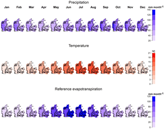
Observed daily values for precipitation, temperature and E_T0 from the Danish Meteorological Institute (DMI) are used (Scharling and Kern-Hansen, 2012). The spatial scale for precipitation and temperature, E_T0, is 10 and 20 km, respectively. However, we assume temperature and E_T0 to be equally distributed within the 20 km and set the same values of the 20 km to the 10 km grid. Then, in total there are 662 (for precipitation) and 724 (for temperature and E_T0) grid points, which cover the 43 000 km² area of Denmark. Moreover, precipitation is corrected for under-catch errors as explained in Stisen et al. (2011) and (2012). The time and spatial variations of the variables can be seen in Fig. 1. Values are monthly accumulations for precipitation and E_T0 and monthly averages for temperature, averaged over the observed record (1990–2013). Danish weather is mainly driven by its proximity to the sea. There is a modest spatial precipitation gradient from west to east, which is more pronounced during autumn and winter. The driest month in terms of precipitation is April and the wettest is October. E_T0 also shows a modest spatial variability during spring and summer, with larger values in eastern Denmark.

Figure 1 Spatiotemporal variability of precipitation (mm month⁻¹), temperature (^∘C) and reference evapotranspiration (mm m⁻¹) of monthly aggregated values (P, E_T0) and monthly averages (T) of the observation period (1990–2013).

2.2 Post-processing strategy

Given the fact that the spatial resolution of the ensemble data differs from the resolution of the observed data, first the ensemble forecasts were interpolated to match the 10 km grid of observed values using an inverse distance weighting (Shepard, 1968), where the values at a given point on the higher-resolution grid (10 km) are computed using a weighted average of the four surrounding nodes of the lower-resolution forecast grid (70 km). The weights are computed as the inverse of the Euclidean distances between the observed grid node and the forecast nodes. Forecasts are then post-processed for each grid point, time of forecast (month) and lead time (month) for each variable separately. Moreover, the computation is done in a leave-one-out cross-validation mode (Wilks, 2011, and Mason and Baddour, 2008) such that the year being corrected is withdrawn from the sample. This is to ensure independence between training and validation data. Then, for example, for precipitation, $\mathrm{662}\times \mathrm{12}\times \mathrm{7}\times \mathrm{24}$ (no. of grid points, no. of months, no. of lead times and no. of years in the sample, respectively) correction models are computed.

2.3 Post-processing methods

2.3.1 Delta method – linear scaling (LS)

The linear scaling approach operates under the assumption that forecast values and observations will agree in their monthly mean once a scale or shift factor has been applied (Teutschbein and Seibert, 2012). LS is the simplest possible post-processing method as it only corrects for biases in the mean. The factor is commonly computed differently for precipitation, E_T0 and temperature due to the different nature of the variables, as precipitation and E_T0 cannot be negative.

For precipitation and E_T0,

$$\begin{array}{}\text{(1)}& f_{k,i}^{*}={\displaystyle \frac{\sum _{j=\mathrm{1}}^{N-\mathrm{1}}{y}_j}{\sum _{j=\mathrm{1}}^{N-\mathrm{1}}{\stackrel{\mathrm{‾}}{f}}_j}}{f}_{k,i}\mathrm{for}i\ne j.\end{array}$$

For temperature,

$$\begin{array}{}\text{(2)}& f_{k,i}^{*}=f_{k,i}-{\displaystyle \frac{\mathrm{1}}{N-\mathrm{1}}}\left[\sum _{j=\mathrm{1}}^{N-\mathrm{1}}{\stackrel{\mathrm{‾}}{f}}_j-\sum _{j=\mathrm{1}}^{N-\mathrm{1}}{y}_j\right]\mathrm{for}i\ne j,\end{array}$$

where f_k,idenotes ensemble member k for k=1, …, M of forecast–observation pair i=1, …, N; M denotes the number of members (15 or 51) and N is the number of forecast–observation pairs; ${\stackrel{\mathrm{‾}}{f}}_j$ denotes the ensemble mean; and y_j denotes the verifying observation. Note that, as stated in Sect. 2.3, both the means of ${\stackrel{\mathrm{‾}}{f}}_j$ and y_j are computed with the sample that withdraws forecast and observation pair i. Finally, $f_{k,i}^{*}$ represents the corrected ensemble member. Note that for precipitation, before applying the correction factor, we set all values of daily precipitation below a specific threshold to zero to remove the “drizzle effect” (Wetterhall et al., 2015). The threshold was chosen so that the number of dry days on a given forecast month matches the number of observed dry days. This threshold varies according to the month and the year and spatially, with an average value of 1.5 mm day⁻¹ over Denmark.

2.3.2 Quantile mapping (QM)

QM relies on the idea of Panofsky and Brier (1968). This method matches the quantiles of the predictive and observed distribution functions in the following way:

$$\begin{array}{}\text{(3)}& f_{k,i}^{*}=G_i^{-\mathrm{1}}\left(F_i\left(f_{k,i}\right)\right),\end{array}$$

where F_i represents the predictive cumulative distribution function (CDF) for forecast–observation pair i, and G_i represents the observed CDF. Again, note that, as stated in Sect. 2.3, both F_i and G_i are computed with a sample that withdraws forecast and observation pair i.

F_i is calculated as an empirical distribution function fitted with all ensemble members of daily values of a given month for a given lead time and grid point. For example, for a forecast of target month June initialized in May, F_i is fitted using a sample comprising 30 (days) × 23 (number of years in the reforecast minus the year to be corrected) × 51 (number of ensemble members). The same is done for G_i, except that the fitting sample is comprised of 30×23 values only. F and G are computed as an empirical CDF. Linear interpolation is needed to approximate the values between the bins of F and G. Extrapolation is then needed to map ensemble values and percentiles that are outside the fitting range. Note that other approaches to deal with values outside the sample range exist that are more suitable when the focus of the study is the extreme values. For example, Wood et al. (2002) fitted an extreme value distribution to extend the empirical distributions of the variables of interest. However, analyzing the effects of different fitting strategies is out of the scope of the present paper.

2.4 Verification metrics

In order to evaluate the raw forecasts and their improvement after post-processing, we analyzed four attributes of forecast quality: bias, skill in regards to accuracy and sharpness, and statistical consistency.

2.4.1 Bias

Bias is a measure of under- or overestimation of the mean of the ensemble in comparison with the observed mean:

$$\begin{array}{}\text{(4)}& \mathit{\%}\mathrm{Bias}=\left({\displaystyle \frac{\sum _{i=\mathrm{1}}^N{\stackrel{\mathrm{‾}}{f}}_i}{\sum _{i=\mathrm{1}}^N{y}_i}}-\mathrm{1}\right)\times \mathrm{100}\end{array}$$

for precipitation and E_T0 and

$$\begin{array}{}\text{(5)}& \mathrm{Bias}={\displaystyle \frac{\mathrm{1}}{N}}\left[\sum _{i=\mathrm{1}}^N{\stackrel{\mathrm{‾}}{f}}_i-\sum _{i=\mathrm{1}}^N{y}_i\right]\end{array}$$

for temperature. f_i and y_i are the same as in Eq. (1).

If the bias is negative, the forecasting system exhibits a systematic underprediction. Conversely, if the amount is positive the system shows an average overprediction. Values closer to 0 are desirable.

2.4.2 Skill

The skill of a forecasting system is the improvement the system has, on average, with respect to a reference system, which could be used instead. For example, climatology for seasonal forecasts or persistence for short-range forecasts. The skill score is computed in the following manner:

$$\begin{array}{}\text{(6)}& \mathrm{Skill}={\displaystyle \frac{{\mathrm{Score}}_{\mathrm{sys}}-{\mathrm{Score}}_{\mathrm{ref}}}{{\mathrm{Score}}_{\mathrm{per}}-{\mathrm{Score}}_{\mathrm{ref}}}},\end{array}$$

where Score_sys, Score_ref and Score_per are the score value of the system to be evaluated, the reference system and the value of a perfect system, respectively. The range of the skill is from −∞ to 1 and values closer to 1 are preferred. In this paper we calculate the skill with respect to accuracy and sharpness. We compute the continuous rank probability score (CRPS) (Hersbach, 2000), as a general measure of the accuracy of the forecast as it contains information on both forecast biases in the mean and spread. The computation of the score is as follows:

$$\begin{array}{}\text{(7)}& \mathrm{CRPS}={\displaystyle \frac{\mathrm{1}}{N}}\sum _{i=\mathrm{1}}^N\underset{-\mathrm{\infty }}{\overset{\mathrm{\infty }}{\int }}{\left[P_i\left(x\right)-H\left(x-y_i\right)\right]}^{\mathrm{2}}\mathrm{d}x,\end{array}$$

where P_i(x) is the CDF of the ensemble forecast for pair i and H(x−y_i) is the Heaviside function that takes the value 1 when x>y_i and 0 otherwise; and y_i and N are, as in Eq. (1), the verifying observation for forecast–observation pair i and the number of forecast–observation pairs, respectively. We made use of the EnsCrps function of the R package SpecsVerification (Siegert, 2015) developed in R version 0.4-1. For the skill with respect to sharpness we use the average along i=1, …, N of the differences between the 25th and the 75th percentiles of each of the ensemble CDFs, P_i.

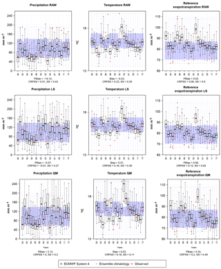
Figure 2 Example of a monthly forecast, valid for August and a lead time of 1 month for a grid point located in west-central Denmark. Blue box plots are the ensemble climatological forecasts. Black box plots are ECMWF System 4 raw or post-processed forecasts. Red dots represent observed values. Bias as in Eqs. (4) and (5) and skill scores for accuracy and sharpness (CRPSS and SS) as in Eq. (8). The first column corresponds to the raw forecast; the second and third columns correspond to the corrected forecasts with the linear scaling or delta change (LS) and quantile mapping (QM) methods, respectively.

In Eq. (6), our reference is ensemble climatology (1990–2013), where the year to be evaluated is withdrawn from the sample. Both the accuracy and sharpness score for a perfect system (see Eq. 6, Score_per) is equal to 0 so the skill score can be then simplified as

$$\begin{array}{}\text{(8)}& \mathrm{Skill}=\mathrm{1}-{\displaystyle \frac{{\mathrm{Score}}_{\mathrm{sys}}}{{\mathrm{Score}}_{\mathrm{ref}}}},\end{array}$$

which, once multiplied by 100, is the percentage of improvement (if positive) or worsening (if negative) over the reference forecast. Throughout the paper, the skill related to accuracy will be denoted as CRPSS whereas the skill due to sharpness will be denoted as SS.

Furthermore, to define the statistical significance of the differences between the skill of ensemble climatology and ECMWF System 4 forecasts, as well as the post-processed predictions, a Wilcoxon–Mann–Whitney test (WMW test; see Hollander et al., 2014) was carried out. The WMW test, unlike the most common t test, makes no assumptions about the underlying distributions of the samples. We applied the test for each grid point, target month and lead time.

Figure 3 Percentage bias and absolute bias of monthly values of raw forecasts. The y axis represents the target month and the x axis represents the different lead times at which target months are forecasted. Values in blue range represent a positive bias and values in red represent a negative bias.

2.4.3 Statistical consistency

We use the probability integral transform (PIT) diagram for a depiction of the statistical consistency of the system. The PIT diagram is the CDF of the z_i's defined as $z_i=P_i(X\le y_i$). Therefore, z_i is the value that the verifying observation y_i attains within the ensemble CDF, P_i. The diagram represents an easy check of the biases in the mean and dispersion of the forecasting system. For a forecasting system to be consistent, meaning that the observations can be seen as a draw of the forecast CDF, the CDF of z_i should be close to the CDF of a uniform distribution on the [0, 1] range. Deviations from the 1:1 diagonal represent bias issues in the ensemble mean and spread. The reader is referred to Laio and Tamea (2007) and Thyer et al. (2009) for an interpretation of the diagram. Similar to Laio and Tamea (2007), we make use of the Kolmogorov bands to have a proper graphical statistical test for uniformity. Finally, we make use of the Anderson–Darling test (Anderson and Darling, 1952) for a numerical test of the uniformity of the PIT diagrams. We carry out the test using the ADGofTest (Gil, 2011) R package (R Core Team, 2017). Here, the null hypothesis is that the PIT diagram follows a uniform distribution on the [0–1] range.

2.5 Accuracy of maximum monthly daily precipitation and number of dry days

For applications such as flooding and forecasting of low flows and droughts, water managers might be interested not only in the skill of monthly accumulated precipitation but also in the skill of other precipitation quantities. We will use a rather simple approach to check for deficiencies of the raw forecasts and whether the post-processing methods improve these deficiencies. We will analyze the improvement in the prediction of monthly maximum daily precipitation and number of dry days in each month. For this study, a dry day is defined as the day with observed zero-precipitation, and the comparison with the ensembles is made daily.

3 Results

3.1 Analysis of raw forecasts

The first row in Fig. 2 depicts the ECMWF System 4 forecast and the ensemble climatological forecast for August accumulated precipitation and E_T0 as well as averaged temperature for one grid located in west-central Denmark for the first month lead time. The values for different forecast qualities for that grid point are also included. For a forecasting system to be useful, it has to be at least better than a climatological forecast. For the given example here, the reference forecast is wider than the ECMWF System 4 forecast. This is an example of a month where we have a slightly better skill than the ensemble climatological forecast for the three variables in question. For example, raw temperature predictions from ECMWF System 4 improve, on average, on the reference forecast by 22 % in terms of accuracy. This level of skill is attained due to the sharper forecasts that exhibit a low bias (−0.23 ^∘C). On the other hand, sharpness is only a desirable property when biases are low. This is illustrated for precipitation forecasts attaining a high skill due to sharpness (0.43) but at the expense of a low skill due to accuracy (0.01). This is caused by the high negative bias (−14.12 %) where, for example for 1992 and 2010, the verifying observation lies outside the ensemble range contributing negatively to the CRPS in Eq. (7).

3.1.1 Bias

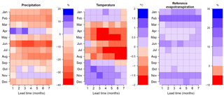
In an effort to summarize the results, a spatial average of the bias throughout Denmark was computed. Figure 3 shows the spatial average bias of precipitation, temperature and E_T0 of the raw forecasts. The y axis represents the target month, for example April, and the x axis represents the forecast lead time – lead time 5 is the forecast for April initiated in December. As we can see from Fig. 3, bias depends on the target month and, to a lesser degree, on lead time. For precipitation, the lowest bias can be found throughout autumn to the beginning of winter, followed by a general underestimation of precipitation that is at its highest for June. April shows an overestimation which might be due to the drizzle effect in a month where dry days are slightly more common, in comparison to March and May (the percentage of dry days within the month is 50 %, 57 % and 56 % in March, April and May, respectively). The drizzle effect issue is a very well-known problem of GCMs and is related to the generation of small precipitation amounts, usually around 1.0–1.5 mm day⁻¹, where observed precipitation is not present (Wetterhall et al., 2015).

Temperature bias averaged over Denmark has a range that lies within [−2, 2] ^∘C. The bias switches from positive to negative when temperatures start to increase in March and from negative to positive bias when temperatures start decreasing in August. This indicates that the forecast of temperature has a smaller annual amplitude than observed. Lowest biases are encountered during January and February with a bias of 0.5 ^∘C, and it is higher during late spring and summer, with a negative bias of almost 2 ^∘C. Finally, the bias range for E_T0 is smaller than precipitation, taking values within [0 %–25 %] on average over Denmark. In general, there is a positive bias, which is at its highest during February.

However, averaging does not tell the whole story. We are also interested in the spatial variation of biases over Denmark. Figure 4 shows the spatial distribution of bias for the first month lead time and its evolution during summer (JJA). In general, there is an underestimation of precipitation throughout Denmark, which much more pronounced during June. Nevertheless, there also exists a positive bias in central Jutland (mid-west Denmark) and on the urban area of Copenhagen (mid-east Denmark) reaching a value around 10 %–20 %. The positive bias area grows in July, occupying most of Jutland and North Zealand (mid-east Denmark).

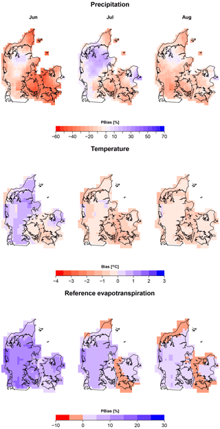
Figure 4 Percentage bias and absolute bias of monthly values of raw forecasts for the summer (JJA). Forecast lead time of 1 month.

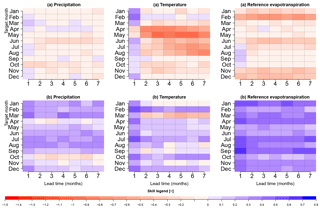
Figure 5 Skill in terms of accuracy (a) and sharpness (b) of monthly values of raw forecasts. The y axis represents the target month and the x axis represents the different lead times at which target month is forecasted.

Other seasons were also mapped and shown in the Supplement as Figs. S1 to S3. During autumn and winter there is also a general negative bias, which is more pronounced in central Jutland, reaching values of −30 %. Nevertheless, an overestimation exists in eastern Denmark for those seasons. For winter, this overestimation is present in the sea grid points. Finally, during spring the spatial variability changes. For example, most grid points exhibit a positive bias during April, except for the southeast region of Denmark that has a small negative bias between 0.0 % and 5.0 %. During May, a tendency of over-forecasting is present in central Jutland.

The spatial distribution of temperature bias during autumn and winter (Figs. S2 and S3, respectively) follows a similar pattern with a general positive bias reaching its highest values in the southeast region (from 1.5 to 2.0 ^∘C). A negative bias is seen during spring (Fig. S1) and late summer across Denmark (Fig. 4). In June, a positive bias of [0–2 ^∘C] is present in a large area of the Jutland peninsula (Fig. 4). Finally, the spatial variation of the bias of E_T0 is less pronounced and, in general, positive. Nonetheless, exceptions exist. There is a negative bias in small regions located in the coastal areas or sea grid points, which ranges from −10 % to 0 %.

The results presented above are specifically for lead time 1, i.e., forecasts of accumulated precipitation and E_T0 and average temperature for August initialized on 1 August. The spatial variation of the bias for other lead times was also mapped (not shown) and analyzed. In general, similar spatial patterns were found for all three variables, being the same along the target months and regardless of lead time.

3.1.2 Skill

Figure 5 summarizes the results for skill in the following manner. First, the values presented are, like in Fig. 3, the spatial average of skill for all of Denmark. Secondly, we evaluate the skill in terms of accuracy (CRPSS, first row) and sharpness (SS, second row). As seen in the evaluation of bias, skill appears to be dependent on the target month and, to a lesser degree, on lead time.

For precipitation, and looking at the first month lead time, ECMWF System 4 skill in accuracy is mildly better than that of climatology for February, March, April, July, August, November and December, with a CRPSS of 0.15 at most. In general, skill in accuracy decreases for lead time 2 onwards. April stands out for having a slightly positive skill in accuracy for almost all lead times, but comes at the expense of having a wider spread than ensemble climatology. For temperature, for the first month lead time, a positive skill exists in terms of accuracy for almost all months, except for late spring. Skill in terms of accuracy also decreases with lead time, but February stands out for having a mild skill for almost all lead times. Forecasts are also in general sharper than ensemble climatology, except for January and March at longer lead times. E_T0 appears to have skill only for late summer and the beginning of autumn in terms of accuracy. This may be explained by the fact that forecasts are sharper than climatology, indicating that there could be an underdispersion issue.

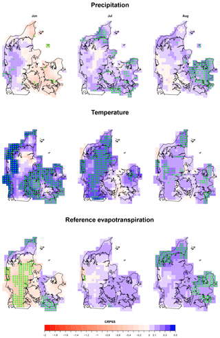
Figure 6 Spatial variability of skill in accuracy for summer (JJA) raw forecasts for a lead time of 1 month. The grids marked with “^*” are points where the distribution of the accuracy for ensemble climatology differs from the accuracy distribution of the ECMWF System 4 forecasts at a 5 % significance using the WMW test.

Note that the computation of the skill score for accuracy was done using a CRPS_sys of 15 or 51 ensemble members, while the CRPS_ref is comprised of 23 members. The disparity in the number of ensemble members can cause forecasts to be at a disadvantage (advantage) compared to a reference forecast with larger (smaller) ensemble size. Ferro et al. (2008) provided estimates of unbiased skill scores that consider the differences in ensemble size. To remove this effect, we calculated the CRPSS using the unbiased estimator for CRPS_ref in Eq. (22) in Ferro et al. (2008). In general, there was a mild increase in the CRPSS value for the months with 15 members, as expected (not shown). The opposite holds for the months with 51 members (February, May, August and November), where a mild decrease in the CRPSS values (not shown) was obtained. Because the changes in CRPSS are moderate, in the rest of the document we will report the results of the CRPSS using the original ensemble sizes (CRPS_sys with 15 or 51 ensemble members, CRPS_ref with 23 members).

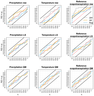
Figure 7 PIT diagrams of summer P, T and E_T0 for the raw and post-processed forecasts for a lead time of 1 month for one grid point located in western Denmark.

Figure 6 shows the skill in accuracy for monthly values and for a lead time of 1 month mapped across Denmark and its monthly evolution during the summer (JJA). The other seasons are also mapped and analyzed and are included in the Supplement (Figs. S4 to S6). Higher skill is observed for temperature, for which ECMWF System 4 improves the ensemble climatological forecast with up to 50 %. Precipitation and E_T0 have lower skill in comparison to temperature, reaching a value of 0.3 for specific months and regions in Denmark. The spatial variation of skill for precipitation seems scattered across Denmark and through the year. Some notable exceptions are the higher skill in accuracy that ECMWF System 4 has in western Jutland during November and December and the low skill attained in October across Denmark (Figs. S5 and S6). The spatial variation of skill in accuracy of monthly averaged temperature seems more pronounced during autumn and spring, with northern Denmark attaining the highest values of skill for these seasons. For the remaining seasons, skill over climatology is present across the country, except for late spring where eastern Denmark has the largest negative skill. Finally, the spatial variation of skill of E_T0 is more pronounced for the months April to November with both positive and negative skill. In general, in this period, eastern Denmark attains positive, although mild for some months, values of skill, except for November.

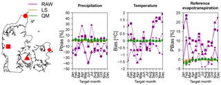
Figure 8 Biases of raw and post-processed precipitation, temperature and E_T0 at four locations in Denmark. Biases are for the different target months and for a lead time of 1 month. Different locations are represented with different symbol shapes according to the map on the left, whereas the raw and the different post-processing techniques are represented with different colors.

In general, the areas with highest biases shown in Fig. 4 are associated with the lowest skill scores. For instance, for precipitation in October in southern central Jutland, the negative bias reaches values around 30 %–40 % (Fig. S2). This leads to values of CRPS almost 60 % smaller than that of ensemble climatology (Fig. S5). The opposite also holds – areas where biases are lower tend to have the highest benefits over ensemble climatology, i.e., precipitation in March across Denmark or in November in western Jutland.

Skill related to accuracy was also mapped for lead times of 2–7 months (not shown). In general, the geographical regions having a statistically significant positive skill score for a lead time of 1 month disappear, except for some smaller regions where a slight positive skill between 0.0 and 0.1 is found, i.e., precipitation in the April forecast initiated in February (lead time of 3 months), which contributes to the mild positive skill at longer lead times as seen in Fig. 5.

The skill related to sharpness was also mapped for all target months and lead times (not shown). In general, forecasts are sharper than ensemble climatology as seen in Fig. 5 across Denmark for all three variables under study. This situation persists, in general, along all lead times, except for precipitation in April and October, in addition to temperature in January, March and November (Fig. 5). For these months, the lack of sharpness is present throughout Denmark. Nevertheless, for precipitation in April, the region with the lack of sharpness is in southern Denmark, along all lead times.

Figure 9 Percentage of grid points with statistically significant positive CRPSS (see Eq. 8).

3.1.3 Statistical consistency of monthly aggregated P, T and E_T0

The first row in Fig. 7 shows the PIT diagram for raw ECMWF System 4 summer forecasts for a lead time of 1 month. The observations and forecast of the diagram come from a grid point located in western Denmark (squared shape in Fig. 8). The remaining seasons can be seen in Figs. S7 to S9. Raw precipitation forecasts, for this grid point, exhibit an underprediction of the mean for winter and autumn and mixed results for the remaining seasons. For example, the underprediction bias is reduced for spring, except for April, where the system exhibits a positive bias. Raw temperature predictions of winter, October and November, in addition to June, exhibit an overprediction, which is lowest for January and February. Spring and summer temperatures exhibit an underprediction, which is highest for July (Figs. S7 and 7). Finally, raw forecasts of E_T0 during all seasons exhibit an overprediction of the mean, in accordance with the results in Sect. 3.1.1. The statistical consistency at longer lead times for all variables (2–7 months, not shown) depends, similarly to bias, on the target month and, to a much lesser degree, on lead time. Temperature in March and, to a lesser degree, precipitation in July exhibit underdispersion issues; i.e., too often the observations lie outside the ensemble range.

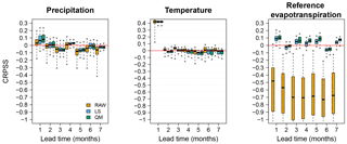
Figure 10 Spatial variability of skill in terms of accuracy for P, T and E_T0 for the raw and post-processed forecasts of February as a target month at different lead times. Box plots represent the values of CRPSS, see Eq. (8) with climatology as reference, of all the 662 or 724 grid points covering Denmark.

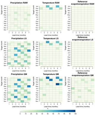
Figure 11 Percentage of grid points for which we fail to reject the null hypothesis of uniformity using the Anderson–Darling test at the 5 % significance level.

Figure 12 Skill of daily monthly maximum P and number of dry days for target month January for all 7-month lead times for the raw and post-processed forecasts. Box plots represent the values of CRPSS, of Eq. (8) with climatology as reference, of all the 662 or 724 grid points covering Denmark.

3.2 Analysis of post-processed forecasts

The second and third rows in Fig. 2 show the corrected forecasts and the bias and skill scores after post-processing using the LS and the QM method, respectively. The results represent a particular grid point and forecast of August initialized on 1 August. After post-processing, the reduction of bias is evident for the three variables under study. Nevertheless, and contrary to what one should expect, this reduction of bias does not necessarily translate into an increase in skill in accuracy, at least for precipitation and temperature and for this month and grid point. The quantification of the reduction of bias and increase in accuracy after post-processing for the whole of Denmark, through the year and for different lead times, is discussed in the Sect. 3.2.2 below.

3.2.1 Bias

Any post-processing technique used should be able to at least remove biases in the mean. This is accomplished using both techniques. Figure 8 shows the bias of precipitation, temperature and E_T0 and its evolution through the year for a lead time of 1 month. Bias is shown for four locations scattered around Denmark. Figure 8 shows that the yearly variability of the bias is collapsed to almost 0 %, although for precipitation and winter E_T0, the LS method seems to be doing slightly better at removing the bias in comparison to QM. This comes as no surprise, as the LS method forces this bias to be zero.

3.2.2 Skill

In order to quantify the improvement over the raw forecast, we compared the number of grid points for which the skill score was positive and negative. Furthermore, the scores are only considered positive or negative if the differences in the distribution of the skill between ensemble climatology and ECMWF System 4 forecasts are statistically significant at the 0.05 level using the WMW test. Consequently, we introduced a third category for which there is no statistically significant difference in skill between climatology and ECMWF System 4 forecasts.

Figure 9 shows the percentage of grid cells with a statistically significant positive skill due to accuracy, Eq. (8), for the raw forecasts (first raw) and the post-processed forecasts (LS, second row; QM, third row). All target months and lead times are included. If a post-processing method is successful in increasing the regions with positive skill scores, then the box for that target month and lead time is bluer in comparison to the raw forecasts. For precipitation, there is no obvious increase in skill due to accuracy, except, perhaps, February and July forecasts for the first month lead time. There are, however, instances for which the percentage of positive skill grid points decreases. The most obvious cases are March and November (first month lead time) with a reduction of almost half, i.e., from 13.6 % (raw) to 5.7 % (LS) for March. On the contrary, temperature and E_T0 exhibit a greater improvement, at least on the first month lead time. For instance, the percentage of grid points with positive skill increases from 4.5 % to 50 % for temperature in April (LS) and from 30 % to 100 % (LS) for temperature in July. The biggest improvement for E_T0 appears in June (first month lead time), reaching 90 % of positive grid cells after post-processing (LS).

In addition, the negative and equal categories were also plotted and included in the Supplement as Figs. S10 and S11. After post-processing, there are instances where a considerable amount of grid cells change from a statistically significant negative skill score to the third category (no significant differences between ensemble climatology and ECMWF System 4 score distributions, Fig. S11). This is true for temperature and E_T0 at longer lead times. One of the obvious examples is February E_T0 at lead time 6 (forecast initiated in September); the percentage of grid points with negative skill scores decreases from 80.5 % to 4.3 % after post-processing (Fig. S10). On the other hand, the percentage of grid points with no significant differences in skill increases from 20 % to 95.7 % after post-processing (Fig. S11) for this example.

To further illustrate the above situation, Fig. 10 shows the variability of the CRPSS when considering all grid points (662 or 724 grid points across Denmark). Figure 10 shows the CRPSS for the target month of February at all lead times and the raw and post-processed skill. The figure shows a reduction of the spatial variability of skill in accuracy and for this month, this reduction is more pronounced for E_T0. However, and as mentioned above, the reduction of spatial variability of accuracy is not enough to ensure statistically significant positive differences in skill.

Results for sharpness (Figs. S12 to S14), similar to Fig. 9, show that a loss of sharpness occurs after post-processing in comparison to raw forecasts for LS and QM applied to precipitation and QM applied to temperature and E_T0. Sharpness seems to be maintained for temperature and E_T0 when we use the LS method. This can be explained by the fact that the correction factor applied to temperature forecasts is additive, which in turn changes the level of the ensemble members and has no effect in the spread of the forecasts, leaving the sharpness score equal to that of the raw forecasts. On the other hand, when the correction factor is multiplicative, as in Eq. (1) for precipitation and E_T0, not only the level but also the spread is affected. It will increase the spread when the correction factor is above 1 (which indicates an underprediction issue) and, conversely, reduce the spread when the correction factor is below 1 (indicating an overprediction issue). The larger the correction factor is, the larger effect it will have in the ensemble spread. For E_T0, where biases are in general lower than biases in precipitation, sharpness seems not to be affected. This effect is somewhat artificial and may lead to misleading evaluations of the power LS has in correcting for biases in spread.

3.2.3 Statistical consistency of post-processed monthly aggregated forecasts

The second and third rows in Figs. 7 and S7–S9 show the PIT diagrams of corrected forecasts for one grid point located in western Denmark. In general, the statistical consistency seems to be improved (points closer to the 1:1 diagonal in Fig. 7) to the same degree for both post-processing methods. Although, for E_T0, this consistency is better enhanced by QM. This fact may be explained by the more evident sharpness loss after correcting forecasts with the QM method (Figs. S11 to S13).

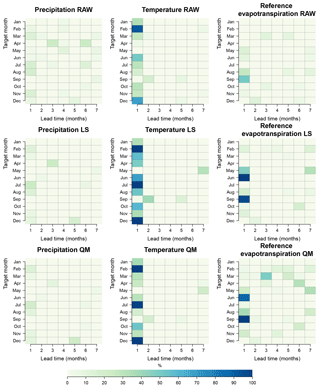
Figure 11. depicts the results of the AD test in the following manner. First, the first, second and third rows represent the results of the raw and post-processed forecasts with LS and QM methods, respectively. Secondly, as for Fig. 9, the x axis represents the lead time and the y axis the target month. Finally, the percentage shows the proportion of grid points for which the null hypothesis of uniformity at the 5 % significance level is accepted. A variety of results are found by the inspection of Fig. 11. First, the percentage of grid points for which the uniformity hypothesis is accepted is very low for raw forecasts. This conclusion holds except for temperature in January and February, with forecasts initialized in months with 51 ensemble members. Secondly, the percentage increases after post-processing for selected months and lead times, usually involving target months with 51 ensemble members. This increase is more visible in post-processed forecasts using the QM method. Finally, the statistical consistency of E_T0 appears to remain low even after post-processing.

3.2.4 Accuracy of extreme precipitation and number of dry days

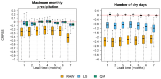
Figure 12 shows the skill in terms of accuracy for both monthly maximum precipitation and the monthly number of dry days. Box plots represent the range of the skill score of all 662 grid cells. Skill scores are for January forecasts for all seven lead times. Two features are highlighted. First, spatial variability of skill gets reduced after post-processing. Secondly, for the skill of the number of dry days, results show that QM performs significantly better than LS. This is not surprising as QM adjusts for biases in the whole range of percentiles of the distributions, whereas LS only focuses on the mean. Note that the apparent increase in skill after LS post-processing is a consequence of the drizzle effect removal before bias correction. Despite the reduction of the spatial variability and an increase, on average, in the skill of post-processed monthly maximum precipitation and number of dry days, results still fail to show an improvement over climatology, as the CRPSS is still negative, even after bias corrections are implemented.

4 Summary and conclusions

The present study had two objectives. The first was to analyze the bias and skill of the ECMWF System 4 in comparison to a climatological ensemble forecast, i.e., a forecast based on observed climatology over a period of 24 years. The second was to compare the statistical consistency between the predictive distribution and the distribution of its verifying observations. This analysis was done for hydrologically relevant variables: precipitation, temperature and E_T0. The conclusions of the first objective of the study and which answer the first question posed in Sect. 1 can be summarized as follows:

• Raw seasonal forecasts of precipitation, temperature and E_T0 from ECMWF System 4 exhibit biases which depend on the target month and, to a lesser extent, on lead time. This result is also in accordance to what was found in Crochemore et al. (2016). There is a persistent over-forecasting issue for E_T0, which can be the result of a combination of biases originating in of both temperature and incoming shortwave solar radiation.

• In general, skill in terms of accuracy is only present during the first month lead time, which is basically the skill of the medium-range forecast. Crochemore et al. (2016) found a similar degree of skill of the raw ECMWF System 4 forecasts for mean areal precipitation in France.

• One seeming advantage ECMWF System 4 has over ensemble climatology is that forecasts are sharper. However, this overconfidence, combined with the biases in the mean, leads to lower levels of accuracy in comparison to the accuracy of the ensemble climatological forecasts. Using the PIT diagrams, we could confirm the results for the bias on the mean of precipitation, temperature and E_T0.

The second objective was to improve the forecasts using two relatively simple methods of post-processing: LS and QM. This was done having in mind the biases GCMs have in the mean and dispersion. Modest improvements were found and can be summarized as follows:

• Both methods perform equally well in removing biases in the mean.

• In terms of accuracy, mild improvements are seen on the first month lead time, especially for temperature and E_T0, where a higher portion of grid points over Denmark can reach a positive skill. Precipitation and longer lead times are still difficult to improve. This may be explained by the same situation as discussed in Zhao et al. (2017). QM performs better when there exists a linear relationship between ensemble mean and observations. This linear relationship may be absent at longer lead times reducing the effectiveness of these methods.

• Looking at the spatial distribution of skill in sharpness we see that for precipitation, both methods tend to decrease it, with a slight increase in QM over LS. For temperature and E_T0, LS seems to be able to keep the sharpness of the raw forecasts. This is not the case for QM, as it manages to make the areas where a slight positive skill is present disappear. Note, however, that sharpness using the LS method is improved when the correction factor is multiplicative and less than 1 (positive bias; i.e., E_T0). The opposite holds: sharpness is inflated when the multiplicative correction factor is greater than 1 (negative bias; i.e., precipitation). This has implications for the computation of the CRPS, as its value increases (decreases) for wider (narrower) ensemble forecasts, on top of the penalization for biased predictions. This situation may also explain why in Crochemore et al. (2016) LS has a better improvement in terms of sharpness than QM, at least for precipitation in spring.

• Statistical consistency is improved using QM. Moreover, QM also performs better in correcting biases of low values of precipitation. This is not a surprising result, as QM corrects for biases for the entire percentile range.

We are aware that our research has limitations. The first is that methods applied here were implemented on a grid-to-grid basis. This may fail to maintain spatiotemporal and intervariable dependencies. Spatial correction methods have been suggested such as the ones used by Feddersen and Andersen (2005) and Di Giuseppe et al. (2013). Another suggestion has been to recover these dependencies by adding a final post-processing step such as the methods proposed in Clark et al. (2004) or Schefzik et al. (2013). The second limitation is the exclusion of post-processing methods tailored to ensemble forecasts, which consider the joint distribution of forecasts and observations (Raftery et al., 2005; Zhao et al., 2017). Their inclusion would gain a deeper insight to the comparison presented here by increasing the complexity of the correction methods and the evaluation of their added value in comparison to simpler approaches.

Post-processing for seasonal forecasting is still a subject at its infancy and, although one could argue that advances in seasonal forecasting will make post-processing unnecessary in the future, there are still opportunities for enhancement. GCMs suffer from several issues as discussed here; however, we still encourage their use. They are physically based, sharper than climatological forecasts. We believe that once bias issues are fixed by means of a more realistic representation of coupled and subgrid processes and/or a better integration of observational data using data assimilation (Weisheimer and Palmer, 2014; Doblas-Reyes et al., 2013), GCMs will be able to provide valuable information at longer lead times for sector applications such as water management.