The development and evaluation of a hydrological seasonal forecast system prototype for predicting spring flood volumes in Swedish rivers

Hydropower makes up nearly half of Sweden's electrical energy production. However, the distribution of the water resources is not aligned with demand, as most of the inflows to the reservoirs occur during the spring flood period. This means that carefully planned reservoir management is required to help redistribute water resources to ensure optimal production and accurate forecasts of the spring flood volume (SFV) is essential for this. The current operational SFV forecasts use a historical ensemble approach where the HBV model is forced with historical observations of precipitation and temperature. In this work we develop and test a multi-model prototype, building on previous work, and evaluate its ability to forecast the SFV in 84 sub-basins in northern Sweden. The hypothesis explored in this work is that a multi-model seasonal forecast system incorporating different modelling approaches is generally more skilful at forecasting the SFV in snow dominated regions than a forecast system that utilises only one approach. The testing is done using cross-validated hindcasts for the period 1981–2015 and the results are evaluated against both climatology and the current system to determine skill. Both the multi-model methods considered showed skill over the reference forecasts. The version that combined the historical modelling chain, dynamical modelling chain, and statistical modelling chain performed better than the other and was chosen for the prototype. The prototype was able to outperform the current operational system 57 % of the time on average and reduce the error in the SFV by ∼ 6 % across all sub-basins and forecast dates.

1 Introduction

The spring flood period (sometimes referred to as the spring melt or freshet period in the literature) is of great importance in snow dominated regions like Sweden where hydropower accounts for nearly half of the country's electrical energy production (Statistiska centralbyrån, 2016). Between 55 and 70 % of the annual inflows to reservoirs in the larger hydropower producing rivers occur during this relatively short period, typically from mid-April/early-May to the end of July. This means that the majority of the annual water resources available for hydropower production would only be available to producers during this period if it were not regulated through carefully planned reservoir management. This reservoir management is important as the energy demand is out of phase with the natural availability of the water resources; typically demand is higher during the colder months when the inflows are lower and vice versa. Therefore the goal is to redistribute the availability of these resources from the spring flood period to other times of the year when electricity demand is higher i.e. during the six months of colder winter, while maintaining the balance between a sufficiently large volume of water for optimal production and enough remaining capacity for safe flood risk management (Olsson et al., 2016). The typical strategy for operators in Sweden is to have reservoirs at around 90 % capacity at the end of the spring flood which is then ideally maintained until the beginning of winter. To achieve this, operators require reliable seasonal forecast information to help them in planning the operations both leading up to and during the spring flood period.

The sources of predictability for hydrological seasonal forecasts come from the initial hydrological conditions i.e. information relating to the water stores within the catchment (e.g. Wood and Lettenmaier, 2008; Wood et al., 2015; Yossef et al., 2013), and also from knowledge of the weather during the forecast period i.e. seasonal meteorological forecasts (e.g. Bennet et al., 2016; Doblas-Reyes et al., 2013; Wood et al., 2015; Yossef et al., 2013). Hydrological seasonal forecasts attempt to leverage at least one of these sources of predictability to make skilful predictions of future streamflow.

In practice, there are two predominant approaches to making hydrological forecasts at the seasonal scale: statistical approaches and dynamical approaches (see Sect. 2.1.4 and 2.1.5 for more information regarding how these approaches were implemented in the context of this work). Statistical approaches utilise empirical relationships between predictors and a predictand, typically streamflow or a derivative thereof (e.g. Garen, 1992; Pagano et al., 2009). These predictors can vary greatly in type from local hydrological storage variables like snow and groundwater storage (e.g. Robertson et al., 2013; Rosenberg et al., 2011), to local and regional meteorological variables (e.g. Còrdoba-Machado et al., 2016; Olsson et al., 2016), or even large scale climate data such as ENSO (El Niño Southern Oscillation) indices (e.g. Schepen et al., 2016; Shamir, 2017). All, however, are trying to leverage the predictability in these predictors that originate from one of the two aforementioned sources. Dynamical approaches use a hydrological model, typically initialised with observed data up to the forecast date so that the model state is a reasonable approximation of the initial hydrological conditions, and then force it with either historical observations (called ensemble streamflow prediction or ESP; e.g. Day (1985)) or using data representative of the future meteorological conditions such as general circulation model (GCM) outputs (e.g. Crochemore et al., 2016; Olsson et al., 2016; Yuan et al., 2013, 2015; Yuan, 2016). Attempts to improve these types of approaches have involved bias adjusting the GCM outputs (e.g. Crochemore et al., 2016; Lucatero et al., 2017; Wood et al., 2002; Yuan et al., 2015), bias adjusting the hydrological model outputs (e.g. Lucatero et al., 2017), or a combination of both (e.g. Yuan and Wood, 2012). Another dynamical approach is the well-established ESP method (Day, 1985). This is similar to the previous approach (GCM); however, instead of using GCM outputs to force the hydrological model it uses an ensemble of historical data. This approach is perhaps one of the most widely used methods and is still the subject of new research. Recent work has looked at conditioning the ensembles before using them, which can be done using GCM outputs (e.g. Crochemore et al., 2016), climate indices, and circulation pattern analysis (e.g. Beckers et al., 2016; Olsson et al., 2016; Candogan Yossef et al., 2017).

The current practice at the Swedish Meteorological and Hydrological Institute (SMHI) for seasonal forecasts of reservoir inflows is the ESP approach. It assumes that historical observations of precipitation and temperature are possible representations of future meteorological conditions and are used to force the HBV hydrological model (e.g. Bergström, 1976; Lindström et al., 1997) to give an ensemble forecast that has a climatological evolution from the initial conditions. A number of attempts have been made in the past to improve the performance of these spring flood forecasts with limited success (Arheimer et al., 2011) demonstrating that these seasonal forecasts are already of a high quality. Work by Olsson et al. (2016) on improving these forecasts was able to realise reasonable improvements using a multi-model approach. By combining a statistical approach, dynamical approach and an analogue approach (conditioned ESP) they were able to show a ∼ 4 % reduction in the forecast error of the spring flood volume (SFV). The purpose of this paper is to continue on and update the work started by Olsson et al. (2016) regarding developing and evaluating a hydrological seasonal forecast system prototype for forecasting the spring flood volumes in Sweden.

This paper is organised as follows. Section 2 outlines the prototype, including the individual model chains, the experimental set-up, the methods and tools implemented, and the study area and data used in this work. Section 3 presents and discusses the cross-validated evaluation scores for the prototype, first with reference to climatology and then with reference to the current operational system that is in use at SMHI. Section 4 concludes with the main findings and a brief outlook for future work.

2 Materials and methods

2.1 The multi-model system and the individual modelling chains

In this section we present the modelling approaches used in this work. These are based on those explored by Olsson et al. (2016) with some modification to facilitate their use in an operational environment. First we briefly present the multi-model prototype (Sect. 2.1.1) followed by a brief overview of the individual modelling chains used in the multi-model and why we chose them (Sect. 2.1.2–2.1.5). For more information regarding the individual modelling chains readers are referred to Olsson et al. (2016) and the accompanying Supplement.

2.2 The multi-model ensemble (ME)

The prototypes developed in this work build on an approach first proposed by Foster et al. (2010), and later improved upon and first tested by Olsson et al. (2016). The aim is to adapt their methodology for use in an operational environment and then evaluate the resulting prototype against the current operational system using cross-validated hindcasts for 84 gauging stations in northern Sweden (see Sect. 2.6). Four different modelling chains were considered when developing the prototype (Sect. 2.1.2–2.1.5). The performances of different combinations of these four were tested. A combination of all four modelling chains was not considered as the analogue model chain is a subset of the historical model chain.

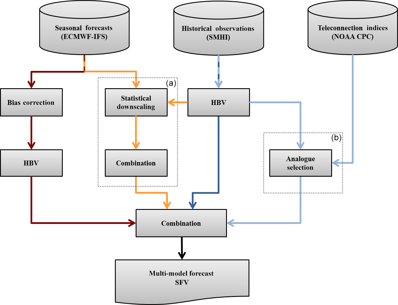
Figure 1 Schematic of the multi-model forecast system. The three individual model chains that are included in the multi-model are (from left to right) the dynamic model chain (red lines), the statistical model chain (orange lines), and the historical (dark blue lines) or analogue (light blue lines) model chain. The dashed boxes labelled (a) and (b) indicate the parts of the system that have non-trivial changes from the multi-model described in Olsson et al. (2016).

Figure 1 shows the generalised schematic of the two prototypes, ME_ads and ME_hds (where the subscripts refer to the individual modelling chains making up each multi-model), including where the current methodologies differ significantly from those in previous works. These differences are discussed in the relevant modelling chain sections below. The prototypes are multi-model ensembles of the outputs from the three respective individual modelling chains. These outputs are pooled together rather than using an asymmetric weighting scheme due to the lack of data points, a total of 35 spring flood events (hindcast period was 1981–2015, see Sect. 2.6), from which to derive a robust weighting scheme. The simple weighting scheme used by Olsson et al. (2016) was tested but, other than improving the ensemble sharpness, did not offer an improvement over the pooling approach.

2.2.1 Historical ensemble (HE)

The historical model chain, the dark blue chain third from the left in Fig. 1, is an ensemble forecast made by forcing a rainfall–runoff model with historical observations of precipitation and temperature. This approach is often referred to as ESP (ensemble streamflow prediction) in the literature but we chose not to as we feel our terminology is more descriptive in the context of this work. This is the current operational seasonal forecasting practice at SMHI. The HBV model (Bergström, 1976; Lindström et al., 1997) is initialised by using observed meteorological inputs (P and T) to force the model up to the forecast date so that the model state reflects the current hydro-meteorological conditions. Then, typically all available historical daily P and T series for the period from the forecast issue date to the end of the forecasting period are used as input to HBV, generating an ensemble of forecasts that are climatological in their evolution from the initial conditions. The historical ensemble (HE) is used as the reference ensemble unless otherwise stated.

The HBV is run one river system at a time and the model outputs are later regrouped into three clusters (Sect. 2.6). Typically only historical data prior to the forecast date are used to force the model, however to allow for a more robust cross validation all data including the years after the forecast date were used (excluding the year in question of course). Unfortunately, the scope of this work did not allow for the recalibration of the HBV model before each cross-validated hindcast. This will potentially inflate the performance of the model for the hindcasts of years that were used in the calibration of the model. This will affect the analogue and dynamical model chains too as they also incorporate the HBV model in their set-up.

2.2.2 Analogue ensemble (AE)

The analogue model chain, the light blue chain furthest to the left in Fig. 1, is a subset of the HE. The hypothesis is that it is possible to identify a reduced set of historical years (an analogue ensemble) that describes the weather in the coming forecasting period better than the full historical ensemble used in HE. In this work the circulation pattern approach used by Olsson et al. (2016) was omitted due to data availability issues making it impractical for operational applications. Additionally, their teleconnection approach was revised to take advantage of the findings by Foster et al. (2018) where they identified which teleconnection patterns are related to the SFV and for which period of their persistence prior to the spring flood this connection is strongest. The teleconnection indices they identified are the Arctic Oscillation (AO) and the Scandinavian pattern (SCA) and the periods of persistence for these indices, expressed as the index mean for the identified period, are the seven and eight months leading up to the spring flood respectively.

The persistence for each teleconnection index is calculated from the beginning of the aforementioned period to one month prior to the forecast date (a limitation imposed by data availability), similarly this was done for all years in the climatological ensemble. If the values of these indices are considered to be coordinates in Euclidean space we define analogue years as those years with positions within a distance of 0.2 units in the Euclidean space from the position of the forecast year. The threshold is a compromise between being small enough to ensure that the climate set-up is indeed similar to the year in question and being large enough to actually be able to capture some analogues from the historical ensemble. The selection of the analogues is done at the regional scale, by cluster (Sect. 2.6), and these selections are applied to the associated sub-catchments in turn.

Similar to the HE, the analogue method makes use of years both before and after the hindcast year for the cross-validated hindcasts.

2.2.3 Dynamical modelling ensemble (DE)

The dynamical model chain, the dark red chain furthest to the left in Fig. 1, is similar to the HE; an adequately initialised HBV model is forced by an ensemble of seasonal forecasts of daily P and T from the ECMWF IFS system 4 (Sect. 2.7). A change to previous work has these daily P and T data bias adjusted first before being used to force HBV. The bias adjustment method used is a version of the distribution based scaling approach (DBS; Yang et al., 2010) which has been adapted for use on seasonal forecast data. DBS is a quantile mapping bias adjustment method where meteorological variables are fitted to appropriate parametric distributions (e.g. Berg et al., 2015; Yang et al., 2010). For precipitation, two discrete gamma distributions are used to adjust the daily seasonal forecast values, one for low intensity precipitation events (⩽ 95th percentile) and another for extreme events (> 95th percentile). For temperature, a Gaussian distribution is used to adjust the daily seasonal forecast values.

Observed (Sect. 2.6) and seasonal forecast (Sect. 2.7) time series of P and T spanning the relevant forecast time frame (e.g. January–July for forecasts initialised in January) and for the reference period 1981–2010 are used to derive the adjustment factors to transform the seasonal forecast data to match the observed frequency distributions. First the precipitation data is adjusted and then the temperature data. The latter is done separately for dry and wet days in an attempt to preserve the dependence between P and T (e.g. Olsson et al., 2011; Yang et al., 2010). Adjustment factors are calculated for each calendar month as the distributions can have different shapes depending on the physical characteristics of the precipitation processes that are dominant. It should be emphasised that the adjustment parameters were estimated using much of the same data to which they were applied. Ideally the parameters would be estimated using data that does not overlap the data which is being adjusted. However, this was not possible in the scope of this work.

There have recently been some criticism voiced regarding the applicability of quantile mapping for bias adjusting seasonal data (e.g. Zhao et al., 2017). This criticism points out that although quantile mapping approaches are effective at bias correction they cannot ensure reliability in forecast ensemble spread or guarantee coherence. Unfortunately, the scope of this work did not allow the testing of other bias adjustment methods but the criticism is noted and further work is planned to address these points.

These bias adjusted data are then converted into HBV inputs by mapping them from their native grid onto the HBV sub-catchments. The mapping is done by areal weighting and the resulting sub-catchment average P and T values are then adjusted to represent different altitude fractions within the catchment. These data are consequently used to force the HBV model from the same initial state as that used in the HE procedure.

No changes to this methodology are needed to accommodate the cross-validated hindcasting as done with the other model chains.

2.2.4 Statistical modelling ensemble (SE)

The statistical model chain, the orange chain second from the left in Fig. 1, is an ensemble forecast produced by downscaling forecasted or modelled large-scale variables (predictors) to the SFV for each cluster (predictand). The downscaling is done using an SVD approach (singular variable decomposition). The predictors are three large scale circulation variables (Sect. 2.7) and the modelled snow depths from the HBV initial conditions. The outputted ensembles of SFV are combined using a simple arithmetic weighting system. The normalised squared covariance between the four predictors and the predictands are ranked for each forecast initialisation date, and weights between 0 and 1 are applied to the different predictors according to their rank. The lowest ranked predictor is assigned a weight of 0.1 ($=\mathrm{1}/\mathrm{10}$), the next lowest predictor is assigned a weight of 0.2 ($=\mathrm{2}/\mathrm{10}$), and so on until all four have been assigned a weight. The reason that an asymmetric weighting scheme is used here is that there is physical support for it. Early in the season the snowpack, which is the majority contributor to the spring flood volume, is a fraction of what it will be and is still accumulating. Therefore, the coming meteorological conditions, which dictate snowpack evolution, are more important earlier on in the season than they are later giving physical support for asymmetric weighting. Additionally, the relative importance of these meteorological predictors with respect to each other differs with time too.

The relative simplicity of the statistical model chain means that it was possible to retrain the model before each hindcast during the cross-validation calculations allowing for no overlap between the calibration and validation periods.

2.3 Defining the spring flood

In previous works the spring flood period has often been defined in terms of calendar months e.g. May–June–July (Nilsson et al., 2008; Foster and Uvo, 2010; Arheimer et al., 2011; Olsson et al., 2016; Foster et al., 2016). This definition of the spring flood period is not ideal as it does not take the interannual and geographical variations in the timing of the spring flood onset into account. In this work we propose an improvement to this practice where we define the spring flood to be the period from the onset date to the end of July.

We define the onset as the nearest local minima in the hydrograph before the date after which the inflows are above the 90th percentile, with reference to the inflows during the first 80 days of the current year, for a period of at least 30 days (Fig. 2). For forecasts made after January i.e. those made in February, March, April, and May, the missing inflow data between the 1 January and the forecast date are filled with simulated inflow data from the HBV model using observed precipitation and temperatures as input data.

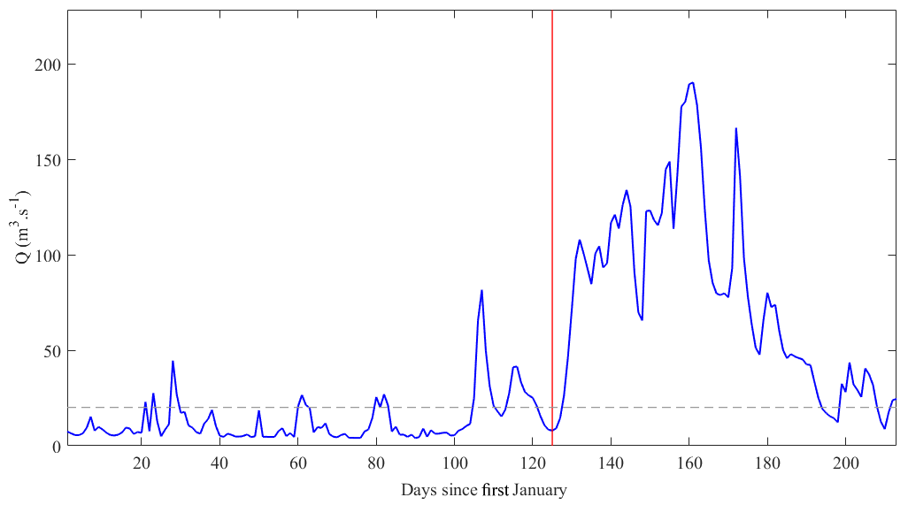
Figure 2 Schematic of how the spring flood is defined. The spring flood is the period between the onset and the last day of July (day 211/212 since the 1 January). The hydrograph from which the spring flood period is to be derived (blue line), the onset date (red line), and the 90th percentile of the inflow for first 80 days (dashed line).

A drawback to this definition is that it is not comprehensive as the end of the spring flood is not defined according to the hydrograph but rather by date. The reason for not defining the end of the spring flood objectively is twofold. Firstly, the forecast horizon for the ECMWF-IFS is seven months which means that forecasts initialised in January may not encompass the entire spring flood period. Secondly, a robust and objective definition of what constitutes the end of the spring flood was difficult to realise within the scope of this work. Further work is needed to resolve this in a more satisfactory manner.

2.4 Experimental set-up

The challenge in this work was to perform a robust evaluation on a limited dataset (35 spring floods, 1981–2015) while minimising the risk of unstable or over fitted statistics. Therefore, a leave-one-out cross-validation (LOOCV) protocol was adopted. Additionally, as it was not practical to recalibrate the HBV model before each step of the LOOCV process; the statistical model uses the same periods for training as those used to calibrate and validate the HBV model. LOOCV is a model evaluation technique that uses n−1 data points to train the models and the data point left out is used for validation. This process is repeated n times to give a validation dataset of length n. This allows for a more robust evaluation with a limited dataset and also gives one the ability to sample more of the variability in the training period than if a traditional validation were performed. The second point is especially advantageous for evaluating the statistical model which is particularly sensitive to situations that were not found within the training period. LOOCV was applied to the individual model chains.

To assess the relative skill for different lead times, we evaluate hindcasts issued on the 1 January (Jan), 1 February (Feb), 1 March (Mar), 1 April (Apr), and 1 May (May) for the spring floods 1981–2015. The evaluation of performance is done in terms of how well the SFV is forecast.

2.5 Evaluation

As it has been mentioned above, we are interested in the ability of a multi-model ensemble's ability to forecast the SFV at differing lead times i.e. forecasts initialised on the first of the month for the months of January through May. It was suggested by Cloke and Pappenberger (2008) that for a rigorous assessment of the quality of a hydrological ensemble prediction system (HEPS) it is not only important to select appropriate verification measures but also to use several different measures so that different properties of the forecast skill can be estimated, resulting in a more comprehensive evaluation.

The evaluations in this paper are designed to answer the following questions:

• Can the forecasts improve on the reference forecast error?

• How often do the forecasts perform better than the reference forecast?

• Are the forecasts better at capturing the interannual variability than the reference forecast?

• Are the forecasts better at discriminating between events and non-events than the reference forecast?

• Are the forecasts sharper than the reference forecast?

• Are the forecasts more sensitive to uncertainty that the reference forecasts?

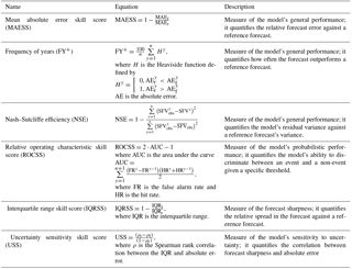
The verification measures used to answer these questions are described below and summarised in Table 1.

Table 1 The validation metrics used to evaluate the multi-model performance. The threshold for skill is 50 for FY⁺ and 0 for all the other metrics.

2.5.1 Mean absolute error skill score (MAESS)

One of the most commonly published scores, even the recommended method, when evaluating HEPS is the continuous rank probability score (CRPS, Hersbach, 2000). However, since we have a limited number of data points, only 35 cross-validated hindcasts per sub-basin, and the CRPS compares distributions, we deemed its use unsuitable for this work. We instead chose to use the mean absolute error (MAE) to evaluate general forecast performance as the CRPS collapses to the MAE for deterministic forecasts (Hersbach, 2000). Therefore, by assuming the ensemble mean to be the deterministic forecast a MAE skill score (MAESS) can be expressed as

$$\begin{array}{}\text{(1)}& {\displaystyle }\mathrm{MAESS}=\mathrm{1}-{\displaystyle \frac{{\mathrm{MAE}}_{\mathrm{f}}}{{\mathrm{MAE}}_{\mathrm{r}}}},\end{array}$$

where f and r denote forecast and reference, respectively. MAE is furthermore defined as

$$\begin{array}{}\text{(2)}& {\displaystyle }\mathrm{MAE}={\displaystyle \frac{\mathrm{1}}{n}}\sum _{y=\mathrm{1}}^n\left|{\displaystyle \frac{{\mathrm{SFV}}_{\mathrm{o}}^y-{\mathrm{SFV}}_{\mathrm{f}}^y}{{\mathrm{SFV}}_{\mathrm{o}}^y}}\right|,\end{array}$$

where y denotes year, n denotes the total number of years, and o denotes observations. The MAESS has a range between negative infinity and one with positive values indicating skill over the reference forecast and a value of one a perfect forecast.

2.5.2 Frequency of years (FY⁺)

In their work Olsson et al. (2016) proposed FY⁺ as a complimentary performance measure to scores such as the MAESS. They are complimentary in that the MAESS is a measure of how much better the forecast is than the reference forecast while FY⁺ is the frequency or how often the forecast is better i.e. how often the absolute error is lower. FY⁺ scores range from 0 to 100 % where values above 50 % indicate that the multi-model forecast has skill over the reference forecast. By assuming the ensemble mean to be the deterministic forecast FY⁺ is expressed as

$$\begin{array}{}\text{(3)}& {\displaystyle }{\mathrm{FY}}^{+}={\displaystyle \frac{\mathrm{100}}{n}}\sum _{y=\mathrm{1}}^n{H}^y,\end{array}$$

where H is the Heaviside function defined by

$$\begin{array}{}\text{(4)}& {\displaystyle }{H}^y=\left\{\begin{array}{c}\mathrm{0},{\mathrm{AbsE}}_{\mathrm{r}}^y<{\mathrm{AbsE}}_{\mathrm{f}}^y\\ \mathrm{1},{\mathrm{AbsE}}_{\mathrm{r}}^y>{\mathrm{AbsE}}_{\mathrm{f}}^y\end{array}\right.\end{array}$$

and AE is the absolute error.

2.5.3 Nash–Sutcliffe model efficiency (NSE)

The NSE (Nash and Sutcliffe, 1970) is a normalised statistic that determines the relative magnitude of the residual variance compared to the measured data variance. The NSE has a range from negative infinity to one with one being a perfect match and values above zero denoting that the forecast has skill over climatology. For this work it can be interpreted as how well the forecasted SFV matches the observed SFV year on year and as such is complimentary to MAESS and FY⁺. By assuming the ensemble mean to be the deterministic forecast the NSE can be expressed as

$$\begin{array}{}\text{(5)}& {\displaystyle }\mathrm{NSE}=\mathrm{1}-{\displaystyle \frac{\sum _{y=\mathrm{1}}^n{\left({\mathrm{SFV}}_{\mathrm{o}}^y-{\mathrm{SFV}}_{\mathrm{f}}^y\right)}^{\mathrm{2}}}{\sum _{y=\mathrm{1}}^n{\left({\mathrm{SFV}}_{\mathrm{o}}^y-{\stackrel{\mathrm{‾}}{\mathrm{SFV}}}_{\mathrm{o}}\right)}^{\mathrm{2}}}}.\end{array}$$

To assess the skill of the multi-model ensemble, with respect to the reference historical ensemble, the difference in their NSE is calculated as

$$\begin{array}{}\text{(6)}& {\displaystyle }\mathrm{\Delta }\mathrm{NSE}={\mathrm{NSE}}_{\mathrm{f}}-{\mathrm{NSE}}_{\mathrm{r}},\end{array}$$

where ΔNSE > 0 indicates that the multi-model forecast has skill over the reference forecast.

2.5.4 Relative operating characteristic skill score (ROCSS)

The ROCSS is a skill score based on the area under the curve (AUC) in a relative operating characteristic diagram. ROCSS values below zero indicate the forecast has no skill over climatology while values over zero indicate skill with one being a perfect forecast. The ROC diagram measures the ability of the forecast ensemble to discriminate between an event and a non-event given a specific threshold. For this work the ROCSS were calculated for the upper tercile (x ⩾ 66.7 %), middle tercile (66.7 % < x ⩽ 33.3 %), and lower tercile (x < 33.3 %). These scores estimate the skill of ensemble forecasts to distinguish between below normal (BN), near normal (NN) and above normal (AN) anomalies. Hamill and Juras (2006) define the ROC skill score to be

$$\begin{array}{}\text{(7)}& {\displaystyle }\mathrm{ROCSS}=\mathrm{2}\cdot \mathrm{AUC}-\mathrm{1},\end{array}$$

where AUC is the area under the curve when mapping hit rates against false alarm rates

$$\begin{array}{}\text{(8)}& {\displaystyle }\mathrm{AUC}=\sum _{y=\mathrm{1}}^{n+\mathrm{1}}{\displaystyle \frac{\left({\mathrm{FAR}}_y-{\mathrm{FAR}}_{y-\mathrm{1}}\right)\left({\mathrm{HR}}_y+{\mathrm{HR}}_{y-\mathrm{1}}\right)}{\mathrm{2}}}\end{array}$$

and FAR is the false alarm rate and HR is the hit rate. False alarms are defined as both the false positive and false negative forecasts, or type I and type II errors. Hits are defined as correctly forecasted events.

2.5.5 Interquartile range skill score (IQRSS) and uncertainty sensitivity skill score (USS)

Sharpness is an intrinsic attribute to HEPS, giving an indication of how large the ensemble spread is. Forecasts ensembles that are too spread are overly cautious and have limited value for an end user due to the uncertainty of the true magnitude of the SFV; conversely ensembles that are not spread enough are overly confident and may not be a true representation of the uncertainty, thus giving the end user false confidence in the forecast (Gneiting et al., 2007). For this work the sharpness is computed as the difference between the 75th and 25th percentiles of the forecast distribution or the interquartile range (IQR). The IQRSS is skill score based on the IQR and is a measure of how much better, i.e. sharper, the forecast ensemble is over the reference ensemble, values above zero indicate that the forecast ensemble is an improvement over the reference ensemble. The IQRSS is expressed as

$$\begin{array}{}\text{(9)}& {\displaystyle }\mathrm{IQRSS}=\mathrm{1}-{\displaystyle \frac{{\mathrm{IQR}}_{\mathrm{f}}}{{\mathrm{IQR}}_{\mathrm{r}}}}.\end{array}$$

As mentioned above, sharpness can be misleading. A well-designed and calibrated ensemble should give the user an idea of the uncertainty of the forecast conveyed through the relative sharpness of the ensemble. Thus it follows that the IQR should be positively correlated to the absolute forecast error; a larger (smaller) IQR would indicate to the user that there is a larger (smaller) uncertainty in the SFV forecast. The uncertainty sensitivity skill score (USS) can be expressed as the skill score of the Spearman rank correlations between the IQR and the absolute deterministic error as follows:

$$\begin{array}{}\text{(10)}& {\displaystyle }\mathrm{USS}={\displaystyle \frac{({\mathit{\rho }}_{\mathrm{r}}-{\mathit{\rho }}_{\mathrm{f}})}{\left(\mathrm{1}-{\mathit{\rho }}_{\mathrm{r}}\right)}},\end{array}$$

where ρ is the Spearman rank correlation.

2.6 Uncertainty estimation

Due to the limited sample size of data available in this work a bootstrap approach is employed to estimate the verification measures and determine whether they are statistically significant. Again due to data limitations a more circumspect significance level is prudent due to the course nature of the resulting statistics; we chose to set the significance level at 0.1 resulting in a 90 % confidence interval between the 5th and 95th percentiles. The cross-validated hindcast ensembles were sampled, allowing for repetition, 10 000 times to calculate the verification measures. We define a result to be statistically significant if the 5th (95th) percentile of the bootstrapped ensemble being evaluated does not overlap the 95th (5th) percentile of the bootstrapped reference ensemble.

2.7 Study area and local data

The sub-basins used in this work are divided into three groups using the clusters defined by Foster et al. (2016), namely clusters, S¹, S², and S³ (Fig. 3). Sweden was divided into five regions of homogeneous streamflow variability: three clusters located in the northern parts of the country, where snow dominates the hydrological processes (northern group); and two located in the southern part, where rain dominates the hydrological processes (southern group). For the purposes of this work we are only interested in the northern group. The numbers of sub-basins in each of these clusters are 25, 19, and 40 respectively. The S in the cluster's designation denotes that the hydrological regimes are dominated by snow processes and the superscripts give the relative strength of the signal from these processes in the hydrological regime. During the winter months most of the precipitation that falls within these basins is stored in the form of a snowpack and does not immediately contribute to streamflow. During the warmer spring months, when the temperatures rise above freezing, these snowpacks begin to melt (typically around mid- to late-April), which results in a period of high streamflow commonly referred to as the spring flood. We focus on forecasts of the accumulated streamflow volume during this period, or SFV.

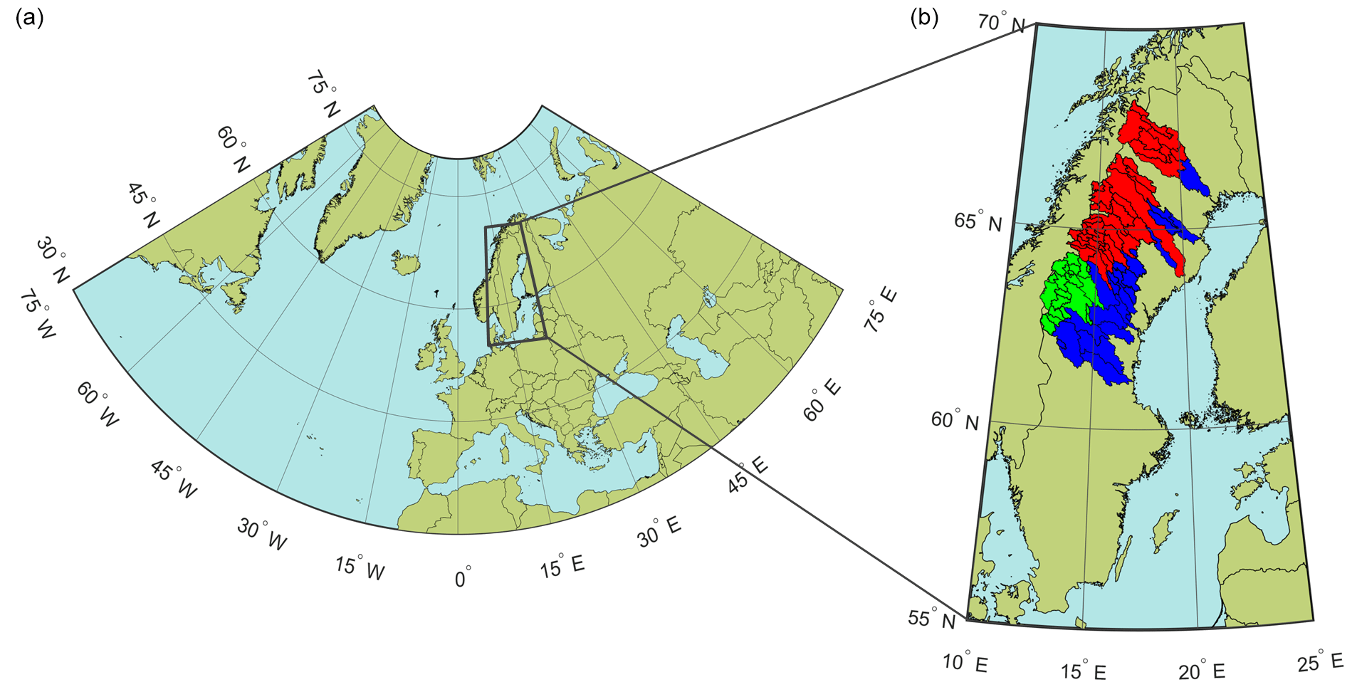
Figure 3 Map showing (a) the domain for the predictors used in the SE modelling chain, (b) the domain of the seasonal forecast data used in the DE modelling chain, and the location of the forecasts sub-basins used in this work. The sub-basins shown in blue belong to cluster S¹, those shown in green belong to cluster S², and those shown in red belong to cluster S³.

For this work, 84 sub-basins from seven hydropower producing rivers in northern Sweden (Fig. 3) were used for the development and testing of the multi-model prototype. The sub-basins utilised include those in the current operational seasonal forecast system at SMHI plus the two unregulated sub-basins used by Olsson et al. (2016). Daily reservoir inflows for each sub-basin are available from the SMHI archives starting from 1961 to the end of the last hydrological year; the data used in our work are for the period 1981–2015 due to some of the other datasets used in this study only being available from 1981. These inflows are derived by adding the local streamflow to the change in reservoir storage then subtracting the streamflow from upstream basins as follows:

$$\begin{array}{}\text{(11)}& {\displaystyle }{Q}_{\mathrm{in}}=\mathrm{\Delta }S+Q_{\mathrm{local}}-Q_{\mathrm{upstream}}.\end{array}$$

Missing inflow data were filled by a multiple linear regression approach using simulated inflows for the sub-basin and observations from the surrounding sub-basins as predictors. Of the 84 sub-basins used in this work 68 had less than 1 % missing data (50 of these had no missing data), four had 1–10 % missing data, five had 20–30 % missing data, four had 30–40 % missing data, and three had 61, 63 and 71 % missing data, respectively. As these sub-basins are a part of the current operational forecast system they were included in the study despite some of them having a significant missing data fraction. The average NSE for the data used for filling was 0.70 (the NSE scores for the intervals above were 0.67, 0.75, 0.77, 0.61, and 0.73, respectively) which suggests that this approach is acceptable.

Daily observations of precipitation and temperature data used in this work were obtained from the PTHBV dataset from SMHI (Johansson, 2002). The PTHBV dataset is a 4×4 km gridded observation dataset of daily precipitation and temperature data that has been created by optimal interpolation with elevation and wind taken into account. These data are available from 1961 to the present.

Table 2 Basic information on the study area including overall performance of the HBV model for the sub-basins in each cluster.

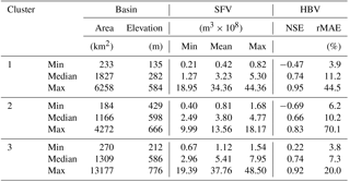
Table 2 gives a summary of some basic basin characteristics and statistics regarding the SFV as well as selected performance measures for the HBV rainfall–runoff model for the sub-basins in each cluster. Although, the ranges in sub-basin areas in the different clusters are similar, except for the maximum in S³, the SFV statistics increase with each cluster when looking from cluster S¹ to S³. This is due to the effects that elevation and latitude have on how much snow processes dominate the hydrological regimes in each cluster. Sub-basins in cluster S¹ are typically at a latitude or elevation lower than those in clusters S² and S³, similarly to the sub-basins in S² with respect to those in S³. The ranges in the NSE and the relative MAE imply that, in general, the HBV model is adequately or well calibrated for most sub-basins, however there are some sub-basins for which the HBV model appears not to be well calibrated and for which there is some scope for improvement. This can be somewhat misleading as these data are a function of three different observations and as such can be subject to noise and uncertainties.

2.8 Driving Data

2.8.1 Teleconnection indices

This work uses monthly indices of the Arctic Oscillation and Scandinavian pattern collected from the Climate Prediction Center (Climate Prediction Center, 2012) for the period October 1960 to May 2015.

2.8.2 Seasonal data

The ECMWF seasonal forecast system model from system 4 (Molteni et al., 2011) is the cycle36r4 version of ECMWF IFS (Integrated Forecast System) coupled with a 1^∘ version of the NEMO ocean model. The seasonal forecasts from the ECMWF IFS were used in the following two different forms: a field of seasonal monthly averages as input to the statistical model, and individual grid points of daily data for input into the HBV model. The choice to use ECMWF data is primarily a practical one. The ECMWF is an established and proven producer of medium range forecasts and SMHI already has operational access to their products.

The seasonal forecast averages are the seasonal means for each ensemble member of the different predictors which had a domain covering 75^∘ W to 75^∘ E and 80 to 30^∘ N (Fig. 2) with a $\mathrm{1}{}^{\circ }\times \mathrm{1}{}^{\circ }$ resolution. For each predictor only the first 15 ensemble members were used in this work. This is because the number of ensemble members available in the ECMWF seasonal forecast is limited to 15 for the hindcast period while the operational seasonal forecast ensemble has 51 members. The predictors considered in this part of the work were the following: 850 hPa geopotential, 850 hPa temperature, 850 hPa zonal wind component, 850 hPa meridional wind component, 850 hPa specific humidity, surface sensible heat flux, surface latent heat flux, mean sea level pressure, 10 m zonal wind component, 10 m meridional wind component, 2 m temperature, and total precipitation.

The daily time series data are the ECMWF IFS seasonal forecasts of daily values of temperature (2mT) and the accumulated total precipitation (pr). These data have a resolution of $\mathrm{0.5}{}^{\circ }\times \mathrm{0.5}{}^{\circ }$, span a period from 1981 to 2015, and have a domain covering 11 to 23^∘ E and 55 to 70^∘ N.

3 Results and discussion

The following section outlines and discusses the results from the cross-valuated hindcasts of the different approaches' ability to hindcast the SFV for the period 1981–2015. First this evaluation is done for each system using climatology as a reference to assess their general skill. Following this the more skilful of the two multi-model ensembles is evaluated using the HE as a reference to assess any improved skill, and thus added value, of the multi-model ensemble approach over the current HE approach. The analysis is carried out on the cross-validated hindcasts of the SFV initialised on the 1 January, February, March, April, and May.

3.1 Evaluating the different forecast systems against climatology

The different forecast approaches' general skill to predict the SFV was estimated using MAESS, their skill to reproduce the interannual variability was estimated using NSE, and finally the skill to discriminate between below BN, NN, and AN SFVs was estimated using ROCSS. Table 3 gives an overview of these scores across all sub-basins and clusters for each initialisation month as well as the percentage of sub-basins where the hindcasts outperformed climatology; the values in brackets are the percentage of sub-basins where the hindcasts outperformed climatology and the result is statistically significant.

Table 3 Bootstrapped (N=10 000) skill scores and the number of sub-basins, as a percentage, where the HEPS performs better than climatology averaged over all 84 sub-basins. The n⁺ values in brackets show the percentages of the sub-basins for which these scores are statistically significant at the 0.1 level.

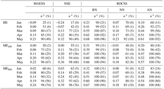
The performance measures for each of the three approaches are positively related to the relative timing of the hindcasts i.e. hindcasts initialised in any month are generally more (less) skilful than the hindcasts initialised in the preceding (following) months. This can be expected as the further away in time from the spring flood that the hindcast is initialised, increasing the lead time, the less the initial hydrological conditions contribute to predictability and the more uncertain the forcing data become (e.g. Wood et al., 2016; Arnal et al., 2017).

With respect to general skill and the ability to capture the interannual variation shown by the observations, the prototypes tend to perform better than HE with ME_hds typically having the best performance. This is especially so when we consider the percentage of the sub-basins where this improved performance is statistically significant. The gap between HE and the two prototypes in MAESS, NSE, and percentage of sub-basins with improved performance over climatology tends to get smaller as the season progresses while the gap in the percentage of sub-basins where improved performance is statistically significant appears to grow, at least early in the season.

However, if we turn our attention to the forecast's ability to discriminate between BN, NN, and AN SFVs then the HE holds an advantage over the two prototypes especially when it comes to identifying NN events from all forecast initialisation dates and, to a lesser extent, BN events for the later forecasts. The proposed prototypes are better at identifying AN events for all forecasts except those initialised in May where the ability of the HE is comparable. The advantage displayed by the HE to identify NN events is to be expected due to its climatological nature while the advantage with respect to BN events can probably be attributed to a cold bias in the historical forcing data caused by climate change. The drop in relative skill by the prototypes in the later forecasts is in part due to their sharpness being worse than the HE in the later forecast (Sect. 3.3).

From these results we are now able to make an informed choice as to which prototype to proceed with, ME_hds (hereafter referred to as the prototype unless stated otherwise). If we take all the results and rank the performances of the three methods then the prototype would rank first, followed closely by ME_ads, and HE would rank third. However, all three forecast methods have been shown to be skilful at forecasting the SFV – albeit a naïve skill.

3.2 Evaluating the prototype against HE

The frequency at which the prototype outperforms HE is estimated using FY⁺, its general skill to predict the SFV is estimated using MAESS, its skill to reproduce the interannual variability is estimated using ΔNSE, and finally its skill to discriminate between BN, NN, and AN SFVs is estimated using ΔROCSS. Figure 4 shows the bootstrapped scores for MAESS, FY+, and ΔNSE calculated for each hindcast initialisation month for the sub-basins in cluster S³. The medians of these bootstrapped scores are presented as a histogram; summary statistics are documented above the histogram. On the left-hand side are the max, mean, and min scores for the cluster i.e. the sub-basins with the highest and lowest scores and the mean for the basin. On the right-hand side are the percentage of sub-basins where the prototype outperformed HE (shows skill over HE $\left(n_{\mathrm{abs}}^{+}\right)$), the percentage of sub-basins where the prototype shows statistically significant skill over HE $\left(n_{\mathrm{0.1}}^{+}\right)$, and the percentage of sub-basins where HE shows statistically significant skill over the prototype $\left(n_{\mathrm{0.1}}^{-}\right)$.

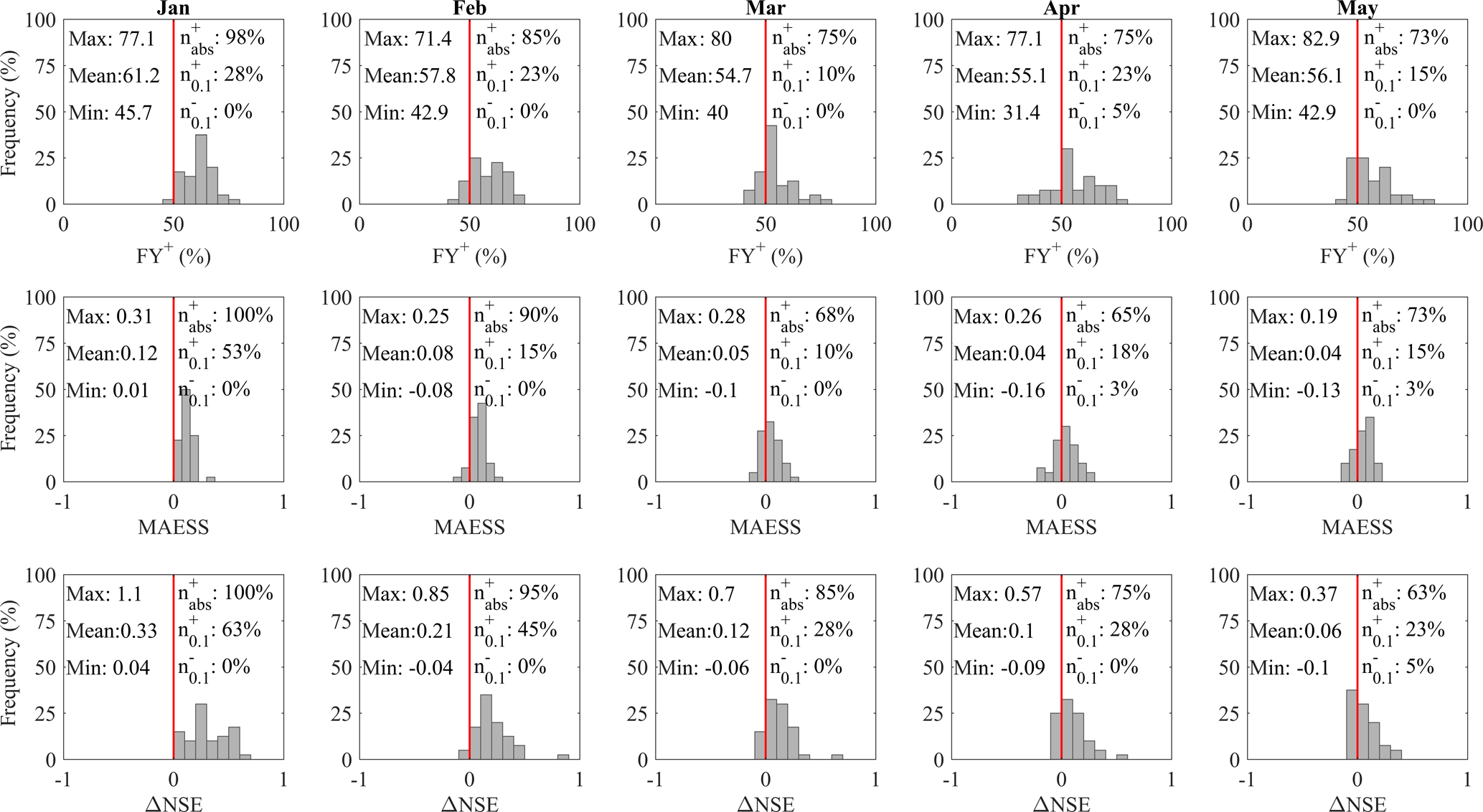
Figure 4 Bootstrapped (N=10 000) FY+, MAESS, and ΔNSE scores for ME_hds with respect to HE for all sub-basins in the cluster S³. Each subplot is a histogram of the medians of the bootstrapped validation scores for each initialisation month. Above the histograms are six related statistics: (left of the red line) the maximum, mean, and minimum of the validation scores shown in the histograms; (right of the red line) percentages of the sub-basins where ME_hds performed better than HE ($n_{\mathrm{abs}}^{+})$, the percentage of sub-basins where ME_hds performed better than HE ($n_{\mathrm{0.1}}^{+})$ at the significance level 0.1, and lastly the percentage of sub-basins where ME_hds performed worse than HE ($n_{\mathrm{0.1}}^{-})$ at the 0.1 level.

3.2.1 FY⁺

The prototype has a FY${}^{+}>\mathrm{50}$ % for the majority of the sub-basins in cluster S³, ranging from 98 % of the sub-basins with a mean FY⁺ of 61 % for hindcasts initialised in January down to 73 % of the sub-basins with a mean FY⁺ of 56 % for hindcasts initialised in May. These figures are similar, even a little higher, for sub-basins in cluster S² while somewhat lower for cluster S¹. The number of sub-basins for which the prototype has a statistically significant FY${}^{+}>\mathrm{50}$ % ranges between 10 and 28 % in cluster S³ (S²=5–37 %, and S¹=12–16 %). Whilst the prototype has a statistically significant FY${}^{+}<\mathrm{50}$ % (performs worse than HE more often than not) for 5 % of sub-basins for hindcasts initialised in April in cluster S³ and 4 % of sub-basins in hindcasts initialised in May for cluster S¹.

3.2.2 MAESS

The prototype shows skill at improving the volume error hindcast by HE for the majority of the sub-basins, ranging between 65 and 100 % of the sub-basins in cluster S³ (S²=74–95 %, and S¹=64–80 %). This improvement tends to be largest for hindcasts initialised in January, mean MAESS of 0.12 (S²=0.11, and S¹=0.04), and lowest for those in May, 0.04 (S²=0.05, and S¹=0.02). The percentage of sub-basins for which MAESS > 0 is statistically significant ranges between 10 and 53 % for all clusters and hindcast initialisations, while the percentage of sub-basins for which MAESS < 0 is statistically significant are 8 and 4 % for hindcasts initialised in March and May in cluster S¹, respectively, and 3 % for hindcasts initialised in both April and May in cluster S³. These results also show that the prototype generally has a smaller MAE than HE especially for earlier hindcast initialisations and again for clusters S³ and S².

3.2.3 ΔNSE

The prototype shows skill at improving the representation of the interannual variability of the observed SFV again for most of the sub-basins, ranging between 63 and 100 % of sub-basins in cluster S³ (S²=74–100 %, and S¹=76–92 %), and the mean ΔNSE ranges between 0.06 and 0.33 for sub-basins in cluster S³ (S²=0.09 and 0.32, and S¹=0.06 and 0.15). The percentage of sub-basins for which ΔNSE > 0 is statistically significant ranges between 16 and 63 % for all clusters and hindcast initialisations, while the percentage of sub-basins for which ΔNSE < 0 is statistically significant are 4 % for hindcasts initialised in January, March, and May in cluster S¹, and 5 % for hindcasts initialised in May in cluster S³.

3.2.4 ΔROCSS

Figure 5, which has the same information presentation structure as Fig. 4, shows the bootstrapped ΔROCSS for the lower (BN), middle (NN), and upper (AN) terciles calculated for each hindcast initialisation month for the sub-basins in cluster S³.

Figure 5 Bootstrapped (N=10 000) ΔROCSS for the lower, middle, and upper terciles between the ME_hds and HE for sub-basins in the cluster S³. Each subplot is a histogram of the medians of the bootstrapped validation score's ensembles for each initialisation month. Above the histograms are six related statistics: (left of the red line) the maximum, mean, and minimum of the validation scores shown in the histograms; (right of the red line) percentages of the sub-basins where ME_hds performed better than HE ($n_{\mathrm{abs}}^{+}$), the percentage of sub-basins where ME_hds performed better than HE ($n_{\mathrm{0.1}}^{+}$) at the significance level 0.1, and lastly the percentage of sub-basins where ME_hds performed worse than HE ($n_{\mathrm{0.1}}^{-}$) at the 0.1 level.

The prototype shows skill over HE to discriminate between BN events and non-BN events for the majority of the sub-basins in cluster S³ for hindcasts initialised in January and February, 95 and 68 % respectively (S²=63, 53 % and S¹=68, 32 %) but this drops to less than half the sub-basins in hindcasts initialised thereafter. The mean ΔROCSS ranges between −0.04 and 0.14 in cluster S³ ($S^{\mathrm{2}}=-$0.03 and 0.05, and $S^{\mathrm{1}}=-$0.06 and 0.02) with only statistically significant results being found in favour of the prototype for 15 and 5 % of sub-basins for hindcasts initialised in January in clusters S³ and S², respectively, and in favour of HE for 4 % of sub-basins for hindcasts initialised in April in cluster S¹.

Out of the three terciles the prototype shows the least skill over HE at discriminating between NN events and non-NN events. The percentage of sub-basins for which the prototype outperforms HE ranges between 23 and 57 % (S²=37–63 %, and S¹=24–60 %) with mean ΔROCSS ranges between −0.07 and 0.01 ($S^{\mathrm{2}}=-$0.06 and 0, and S¹ = −0.05 and 0.02) and no statistically significant results for any sub-basins, both in favour of or against the prototype.

The prototype shows the best performance when discriminating between AN events and non-AN events. The percentage of sub-basins for which the prototype shows skill over HE in the upper tercile ranges between 85 and 98 % for hindcasts initialised in the first three months (S²=47–89 %, and S¹=48–84 %) then 57 and 25 % for the last two months, respectively (S²=63 and 53 %, and S¹=80 and 32 %). The mean ΔROCSS ranges between −0.02 and 0.13 ($S^{\mathrm{2}}=-$0.01 and 0.14, and $S^{\mathrm{1}}=-$0.01 and 0.07). The percentage of sub-basins in cluster S³ for which ΔROCSS > 0 is statistically significant are 18, 10, and 3 % for hindcasts initialised in January, February, and March respectively, and 16 % for forecasts initialised in January and February in cluster S². There are no statistically significant results in favour of HE.

3.3 Analysis of the forecast ensemble sharpness

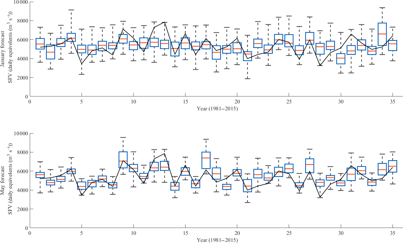
Figure 6 The cross-validated hindcasts of the SFV for a sub-basin in cluster S³ made by ME_hds (boxplots) together with the observed SFV (black line). The box plots represent the entire forecast ensemble, the red lines represent the ensemble medians, the blue boxes the 25th and 75th percentiles (IQR), and the feelers represent the 0th and 100th percentiles.

Figure 6 shows the cross-validated hindcasts by the prototype initialised in January (top panel) and May (bottom panel) for Göuta-Ajaure, a cluster S³ sub-basin in upper reaches of the Ume River system. This basin was chosen as an example of a where the prototype showed typical performance results i.e. neither the best nor the worst. The total ensemble spread (the whiskers) of the forecasts initialised in January remains somewhat consistent from year to year while the IQR (the blue boxes) displays a more pronounced variation. The lack of variation in total spread is primarily the result of the climatological nature of the HE component which tends to have a larger and more consistent spread than that for DE and SE at longer lead times. The greater variation exhibited by the IQR is mostly due to the ”true” forecast nature of the DE and SE components in the multi-model ensemble. If we turn our attention to the forecasts initialised in May we see a more pronounced variation in both the total spread and the IQR. This is because the spread in the DE and SE components is now comparable to and often larger than the spread in the HE component. Table 4 shows how the IQRSS drops as the spring flood season approaches. It can also be seen in Fig. 6 that the ensemble median (red line) is more responsive to the year on year variation in SFV in the May forecasts than in the January forecasts. This is because the relative contribution to predictability by the initial conditions is greater than the contribution from the meteorological drivers closer to the spring flood period. These patterns are generally true for both the forecasts initialised in the intermediate months and for the other sub-basins.

Table 4 Bootstrapped (N=10 000) USS and IQRSS for ME_hds using HE as a reference, and the percentage of sub-basins where ME_hds performed better than HE. The n⁺ values in brackets show the percentages of the sub-basins for which these scores are statistically significant at the 0.1 level.

Figure 7 Maps of the median bootstrapped FY⁺ values for each of the initialisation dates.

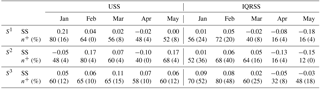
If we assume that the more sensitive an ensemble is to uncertainty the more the forecast sharpness will vary. We would therefore expect the USS values to generally be positive i.e. that the forecast sharpness of prototype is better correlated with the forecast error than for HE. This is largely supported by the USS values in Table 4 where only three values are negative, the January forecast in cluster S² and the April forecasts in both clusters S¹ and S², and even then not by very much. This suggests that at least one but probably both of the DE and SE ensembles are responsible for this improvement due to their variability. There is a general decreasing trend with initialisation date in the USS values in clusters S¹ and S² (if we ignore the value for January in S²) while the values are more consistent in cluster S³. All the uncertainty correlation values for both the HE and the prototype are significant at the 0.1 level (not shown for brevity) suggesting that both exhibit sensitivity to uncertainty to some extent, however the prototype is more sensitive to uncertainty which should instil more confidence in the forecast for the users.

The IQRSS values show that the prototype tends to produce sharper forecasts than HE early in the season i.e. for forecasts initialised in January and February in cluster S¹ and forecasts initialised in January, February, and March in clusters S² and S³. This is reversed for the remaining initialisation dates where HE tends to produce sharper forecasts than the prototype. This is probably due to the climatological nature of the HE having less of an impact on forecast sharpness as the initialisation date approaches the spring flood period in combination with the uncertainties and biases in the other individual ensembles, which further exacerbate the situation.

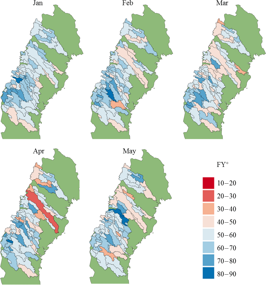
3.4 Spatial and temporal variations and transferability of the prototype

Both multi-model ensembles show skill at forecasting SFV with respect to forecast error, ability to reproduce the interannual variability in SFV, and the ability to discriminate between BN, NN, and AN events. The prototype, in particular, is at worst comparable to the HE and at best clearly more skilful. This relative performance of the prototype varies both in space and time. Figure 7 shows maps of the median bootstrapped FY⁺ values. For hindcasts initialised in January the spatial pattern in the FY+ scores show that the prototype tends to outperform HE more in sub-basins that have a higher latitude or elevation. However, as the initialisation date approaches the spring flood period this pattern becomes less and less coherent. This general pattern is also true for MAESS scores. This suggests that the change in the performances of the prototype and HE, as a function of initialisation date, are not always similar for sub-basins that are near one another. Further work would be needed to find out what the underlying reason for this is.

Data availability is the biggest limiting factor to the transferability of this approach to other areas. The HE, AE, and SE approaches are all dependant on good quality observation time series. Additionally, the skill of all three of these approaches would be expected to be affected by the length of these time series. They length of the time series should be long enough to be a good representative sample of the climatology otherwise the forecasts would be biased in favour of the climate represented in the data and not the true climatology.

The SE and AE approaches require an understanding of how the variability in the local hydrology is affected by large scale circulation phenomena such as teleconnection patterns to help select predictors and teleconnection indices for inputs to each approach, respectively. The hydrological rainfall–runoff model used in the prototype should not pose a problem, although HBV has been successfully set up for snow dominated catchments outside of Sweden (e.g. Seibert et al., 2010; Okkonen and Kløve, 2011), any sufficiently well calibrated rainfall–runoff model would suffice.

We believe that, if the above requirements are met, a seasonal hydrological forecast system similar to the prototype can be set up in other snow dominated regions around the world.

4 Conclusions

In this paper we present the development and evaluation of a hydrological seasonal forecast system prototype for predicting the SFV in Swedish rivers. Initially, two versions of the prototype, ME_ads and ME_hds, were evaluated together using the HE using climatology as a reference for both, to help select which version of the prototype to proceed with and to get a general impression of their skill to forecast the SFV. Thereafter the chosen prototype was evaluated using HE as a reference and finally the sharpness of the hindcast ensembles were analysed.

The main findings are summarised as follows:

• The prototype is able to outperform the HE approach 57 % of the time on average. It is at worst comparable to the HE in forecast skill and at best clearly more skilful.

• The prototype is able to reduce the forecast error by 6 % on average. This translates to an average volume of 9.5×10⁶ m³.

• The prototype is generally more sensitive to uncertainty, that is to say that the ensemble spread tends to be more correlated with the forecast error. This is potentially useful to users as the ensemble spread could be used as a measure of the forecast quality.

• The prototype is able to improve the prediction of above and below normal events early in the season.

Looking forward, future studies need to address the questions raised by Zhao et al. (2017) regarding the bias adjustment of meteorological seasonal forecast data using quantile mapping. Results from this study show that while the seasonal forecasts were bias adjusted the performance of the DE was disappointing; however it still had value within the multi-model setting suggesting that it has more of a modulating roll on the other modelling chains as opposed to contributing directly to predictability.

How the individual model ensembles are combined to give the multi-model output needs to be revisited. When we applied the asymmetric weighting scheme proposed by Olsson et al. (2016) we did not find that it improved the multi-model performance in general across all stations and forecasts and so we did not use it. However, we do believe that more work should be done to find a more appropriate weighting scheme than simple pooling. Perhaps better understanding how the performance of the different modelling chains are affected by the initial conditions and lead time will shed more light on how to best approach this issue. Further development and testing along these lines are planned for the future.

The AE approach did not exhibit the promising performance found by Olsson et al. (2016) using circulation pattern analysis to select the analogues. A part of the explanation for this poor performance is that the teleconnection information used to select the analogues only partially span the full periods identified by Foster et al. (2016), from October/November to the beginning of the spring flood. The missing data could be filled by making forecasts of the indices. Another approach would be to revisit the circulation pattern analysis based approach now that data inhomogeneity issues are largely addressed by the new ERA5 reanalysis data that is becoming available (http://climate.copernicus.eu/products/climate-reanalysis, last access: 15 September 2017). Yet another approach would be to use GCM forecasts to select the analogues (e.g. Crochemore et al., 2016).

Lastly, the post processing of model outputs (e.g. Lucatero et al., 2017) has been shown to be beneficial, the incorporation of a simple approach like linear scaling is possibly the most appealing due to its ease of implementation in an operational environment.