the Creative Commons Attribution 4.0 License.
the Creative Commons Attribution 4.0 License.
 | 29 Mar 2018
Benchmarking ensemble streamflow prediction skill in the UK
Christel Prudhomme
Simon Parry
Katie Smith
Maliko Tanguy
Skilful hydrological forecasts at sub-seasonal to seasonal lead times would be extremely beneficial for decision-making in water resources management, hydropower operations, and agriculture, especially during drought conditions. Ensemble streamflow prediction (ESP) is a well-established method for generating an ensemble of streamflow forecasts in the absence of skilful future meteorological predictions, instead using initial hydrologic conditions (IHCs), such as soil moisture, groundwater, and snow, as the source of skill. We benchmark when and where the ESP method is skilful across a diverse sample of 314 catchments in the UK and explore the relationship between catchment storage and ESP skill. The GR4J hydrological model was forced with historic climate sequences to produce a 51-member ensemble of streamflow hindcasts. We evaluated forecast skill seamlessly from lead times of 1 day to 12 months initialized at the first of each month over a 50-year hindcast period from 1965 to 2015. Results showed ESP was skilful against a climatology benchmark forecast in the majority of catchments across all lead times up to a year ahead, but the degree of skill was strongly conditional on lead time, forecast initialization month, and individual catchment location and storage properties. UK-wide mean ESP skill decayed exponentially as a function of lead time with continuous ranked probability skill scores across the year of 0.75, 0.20, and 0.11 for 1-day, 1-month, and 3-month lead times, respectively. However, skill was not uniform across all initialization months. For lead times up to 1 month, ESP skill was higher than average when initialized in summer and lower in winter months, whereas for longer seasonal and annual lead times skill was higher when initialized in autumn and winter months and lowest in spring. ESP was most skilful in the south and east of the UK, where slower responding catchments with higher soil moisture and groundwater storage are mainly located; correlation between catchment base flow index (BFI) and ESP skill was very strong (Spearman's rank correlation coefficient =0.90 at 1-month lead time). This was in contrast to the more highly responsive catchments in the north and west which were generally not skilful at seasonal lead times. Overall, this work provides scientific justification for when and where use of such a relatively simple forecasting approach is appropriate in the UK. This study, furthermore, creates a low cost benchmark against which potential skill improvements from more sophisticated hydro-meteorological ensemble prediction systems can be judged.
- Article
(5804 KB) - Full-text XML
-
Supplement
(396 KB) - BibTeX
- EndNote


Skilful hydrological forecasts at sub-seasonal to seasonal lead times would provide a valuable tool for improved decision making for wide range of sectors such as water resources management (Anghileri et al., 2016), hydropower operations (Hamlet et al., 2002), and agriculture (Letcher et al., 2004), particularly in times of slow onset events such as drought (Simpson et al., 2016). One of the earliest operational hydrological forecasting methods is ensemble streamflow prediction (ESP). ESP was pioneered in the US at the National Weather Service (NWS) during the 1970s and 1980s as a means of providing ensemble forecasts of streamflow for a variety of lead times from 1 day to seasonal and beyond (Day, 1985; Twedt et al., 1977; originally stood for Extended Streamflow Prediction). Two years of severe drought in California in 1976 and 1977 provided the motivation for such hydrological forecasting developments at the time (Wood et al., 2016b). In the UK, the 2010–2012 drought in England and Wales provided the impetus for the establishment of the first operational seasonal hydrological forecasting service, the Hydrological Outlook UK (HOUK), which went live in June 2013 (Prudhomme et al., 2017; forecasts available at: http://www.hydoutuk.net/). ESP is used as one of three hydrological forecasting methods in HOUK and also feeds into the Environment Agency's monthly “Water Situation Report for England” (operational for groundwater levels in March 2012), providing forward look ESP forecasts of streamflow for 29 catchments out to a 12-month lead time (https://www.gov.uk/government/collections/water-situation-reports-for-england).
In the traditional formulation of ESP, as used in this paper, historical sequences of climate data (precipitation, potential evapotranspiration, and/or temperature) at the time of forecast are used to force hydrological models, providing a plausible range of representations of the future streamflow states. The source of ESP skill is therefore due to initial hydrologic conditions (IHCs) from antecedent stores of soil moisture, groundwater, snowpack, and channel streamflow itself (Wood et al., 2016a; Wood and Lettenmaier, 2008) which can be detectable up to a year ahead (Staudinger and Seibert, 2014), rather than from skilful atmospheric forecasts. The original operational concept of the NWS ESP forecasting system was that it was flexible, easy to use, and could be run efficiently using simple conceptual hydrological models (Day, 1985). Traditional ESP, while simple, is still widely used today in operational seasonal hydrological forecasting (e.g. US NWS and HOUK) and as a low cost forecast against which to benchmark potential skill improvements from more sophisticated hydro-meteorological ensemble prediction systems (e.g. Arnal et al., 2017; Crochemore et al., 2017; Pappenberger et al., 2015; Thober et al., 2015; Wood et al., 2005).
Several studies have established the skill of the ESP method for catchments in particular regions based on carefully constructed hindcast experiments. For example, in the western US, Franz et al. (2003) found ESP forecasts in 14 snow dominated catchments were, on average, skilful (compared to benchmark climatology forecasts) with a lead time up to 7 months, particularly when initialized early in the spring snowmelt season. Wood and Lettenmaier (2008) found that information about IHCs was more important than climate information during the transition between wet and dry seasons in two western US catchments up to a 5-month lead time. For non-snow dominated catchments in the south-east of the US, Li et al. (2009) showed that harnessing the long memory of soil moisture and groundwater stores can provide skilful ESP forecasts, as the impact of anomalous dry or wet conditions can take weeks or months to dissipate. Wang et al. (2011) found simple conceptual rainfall-runoff models were able to reliably estimate conditional catchment IHCs in two east Australian catchments, subsequently producing ESP forecasts of comparable skill to the current operational Bayesian Joint Probability statistical forecast system (BJP, Wang et al., 2009) at 1- and 3-month lead times. More recently, Singh (2016) assessed the potential for long-range ESP forecasting for integrated water management in four catchments (two rainfall dominated and two snowfall dominated) on the South Island of New Zealand and found ESP to be skilful out to a 3-month lead time, with greatest improvements over climatology forecasts in summer. The previous studies demonstrate that the traditional ESP method is skilful at both short and long lead times in many regions around the world and, given its relative ease of application and low computational cost, remains a valuable ensemble hydrological forecasting approach. Although ESP is being used operationally within the UK, its skill has not yet been investigated at the catchment scale within a rigorous hindcast experiment and is therefore the focus of this paper.
By definition, a forecast can only be considered skilful if it is more accurate against observations than some simpler and/or cheaper reference or benchmark forecast (Jolliffe and Stephenson, 2003; Wilks, 2011). Pappenberger et al. (2015) identified three classes of benchmark forecasts commonly used in hydrological forecasting: (i) climatology, used for seasonal forecasting, (ii) persistence, used for short range forecasting, and (iii) simplified hydrology models, for testing whether more complex models provide useful skill gains. We define the process of benchmarking as establishing the skill of a forecasting system (here ESP) against a simpler benchmark forecast across various lead times, forecast initialization months, and for a large sample of diverse catchments within the study domain. Consequently, the aim of this paper is to establish the skill of the traditional ESP method for forecasting streamflow in the UK at the catchment scale using (streamflow) climatology as the benchmark forecast within a rigorous 50-year hindcast study design. Three key research questions emerge:
-
When is ESP skilful, in terms of a wide range of lead times and forecast initialization months?
-
Where is ESP skilful, in terms of spatial distribution of skilful forecasts both regionally and at the individual catchment scale across the UK?
-
Why is ESP skilful, in terms of individual catchment storage capacity?
Section 2 describes the hydroclimatic data used and the selection of catchments, Sect. 3 outlines the methods leading to the generation of ESP hindcasts. Results are presented in Sect. 4 and discussed in Sect. 5, before key conclusions and avenues for further work are offered in Sect. 6. Details about how to access the ESP hindcast archive used in this study as well as supplementary data and figures are given in the “Data availability” section at the end of the article.
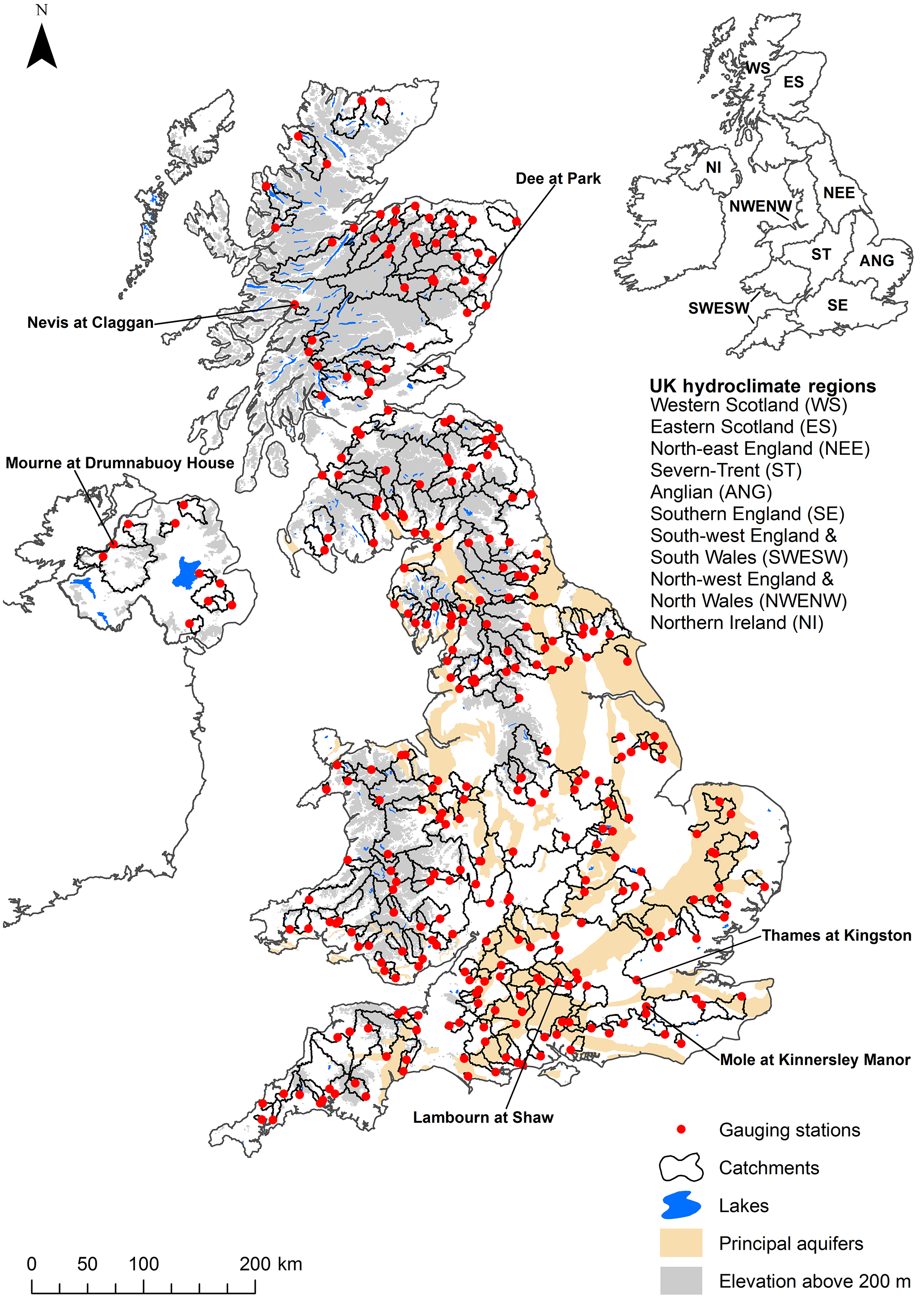
Figure 1Location of 314 gauging stations (red dots) and catchment boundaries (black lines) with upland areas (shaded in grey) and principal aquifers (shaded in pale yellow). UK Hydroclimate Regions, derived from grouping smaller UK hydrometric areas, are shown inset.
We selected a set of 314 catchments for our ESP evaluation from the UK National River Flow Archive (NRFA; http://nrfa.ceh.ac.uk/), chosen to be representative of the range of UK hydroclimatic conditions and ensuring good spatial coverage (Fig. 1). These catchments include those used for routinely assessing the current and future UK hydrological status (e.g. National Hydrological Monitoring Programme, 2017) as well as 128 catchments that are part of the new version of the UK Benchmark Network (UKBN2; Harrigan et al., 2017) that can be considered relatively free from human disturbances such as water abstractions, urbanization, and reservoir impacts. Individual details of all 314 catchments are given in the Supplement Table S1.
Observed catchment average daily mean streamflow Q (m3 s−1), daily precipitation P (mm d−1), and daily potential evapotranspiration ETp (mm d−1) were extracted for each catchment and are needed for three tasks: (i) as input to the hydrological model calibration (Q, P, and ETp; Sect. 3.1); (ii) to generate historic climate sequences (P and ETp, Sect. 3.2) used as forcing to the ESP method; and (iii) as forcing to the reference simulation (P and ETp; i.e. proxy observations in Sect. 3.3).
Q was retrieved from the NRFA over the longest possible period of observed Q across the 314 stations, 32 water years from 1983 to 2014 (water year from 1 October to 30 September referred to by the calendar year in which it ends). P was retrieved from the 1 km gridded CEH-GEAR dataset (Keller et al., 2015; Tanguy et al., 2016) between 1961 and 2015 for the UK. ETp according to Penman–Monteith for FAO-defined well-watered grass was retrieved from the 1 km gridded CHESS-PE dataset (Robinson et al., 2016, 2017) between 1961 and 2015 for catchments in Great Britain. CHESS-PE does not cover Northern Ireland, so an alternative 5 km ETp dataset for the UK based on the temperature-based McGuinness–Bordne equation was used for these 10 catchments instead (Tanguy et al., 2017, 2018).
Table 1Summary statistics of eight catchment characteristics for the UK and nine hydroclimate regions shown in Fig. 1. The median across n catchments within each region is given with the 5th and 95th percentile ranges in parentheses. Area, median elevation, and base flow index (BFI) were retrieved from the UK NRFA. Mean annual Q, P, and ETP were calculated over water years 1983–2014 using data in Sect. 2. RR is the runoff ratio and ∗ is the long term (water years 1983–2014) mean fraction of precipitation that has fallen as snow.
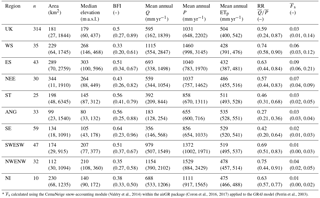
∗ calculated using the CemaNeige snow-accounting module (Valéry et al., 2014) within the airGR package (Coron et al., 2016, 2017) applied to the GR4J model (Perrin et al., 2003).
Catchment characteristics are summarized in Table 1 for the UK and nine hydroclimate regions as shown in Fig. 1 inset. The nine UK Hydroclimate Regions were derived by merging contiguous UK hydrometric areas (National River Flow Archive, 2014) that reflect broad hydrological and climatological similarity across the UK and are used for aiding interpretation of results. The distribution of the 314 catchments within the nine regions varies between 10 in Northern Ireland (NI) and 59 in Southern England (SE). Catchment areas range from 4.4 to 9948 km2 with a median area of 181 km2. There is a distinctive hydroclimatic gradient in the UK with wetter more responsive upland catchments in the north and west, and drier lowland catchments in the south and east, many of which drain the principal Chalk and Limestone aquifers. The slow flow contribution from groundwater and other delayed sources, such as lakes, snow, and soil water storage, was characterized using the base flow index (BFI; Gustard et al., 1992) obtained from UK NRFA metadata. BFI ranges between 0 and 1 with values ∼ 0.15–0.35 representative of more responsive rainfall-runoff regimes in the north and west whereas many Chalk rivers in the south east have a BFI ≥ 0.9. Three regions (Severn-Trent (ST), Anglian (ANG), and SE) have median runoff ratios (RR) < 0.5 meaning more precipitation is lost to evaporation than runoff in the majority of these catchments. Less than 5 % of catchments have a significant amount of snowfall, defined here following Berghuijs et al. (2014) as catchments with a long-term mean fraction of precipitation falling as snow > 0.15, and are mainly situated in Eastern Scotland (ES). The range of these hydroclimatic characteristics provide a large and diverse set of catchments to benchmark ESP skill.
3.1 Hydrological modelling
The first of four key methodological steps was to calibrate and evaluate the GR4J (Génie Rural à 4 paramètres Journalier) model (Perrin et al., 2003) used for the generation of streamflow series. It is a daily lumped catchment rainfall-runoff model with a parsimonious structure consisting of four free parameters that require calibration against streamflow observations using daily P and ETp as input. GR4J has been shown to reliably simulate the hydrology of a diverse set of catchments (Perrin et al., 2003) including temporal transition between wet and dry periods (Broderick et al., 2016), and for the generation of ESP forecasts (e.g. Pagano et al., 2010). The GR4J structure includes a soil moisture accounting reservoir (capacity controlled with parameter X1 [mm]), a water exchange function (rate controlled by parameter X2 [mm d−1]), and a non-linear routing store to represent baseflow (capacity determined by parameter X3 [mm]), with rainfall-runoff time lags (set in days by parameter X4 [d]) controlled by two unit hydrographs.
GR4J was calibrated using the open source “airGR” package v1.0.2 in R (Coron et al., 2016, 2017) with the inbuilt calibration optimization algorithm based on a steepest descent local search procedure and default parameter ranges. The modified Kling–Gupta efficiency (KGEmod; Gupta et al., 2009; Kling et al., 2012) applied to root squared transformed flows KGEmod[sqrt] was used as the objective function for automatic fitting, thus placing weight on mid-range flows, rather than high or low flows. This was decided given ESP forecasts are made across the year during both dry and wet conditions. A split sample test (Klemeš, 1986) was used by dividing the 32-year complete period (CP; water years 1983–2014) of available streamflow observations into two equal 16-year segments for calibration and evaluation: period 1 (P1; water years 1983–1998) and period 2 (P2; water years 1999–2014). Three calibrated GR4J parameter sets were created for each catchment using data from P1, P2, and CP, thus allowing testing of parameter stability between P1 and P2. Model performance against streamflow observations was evaluated using KGEmod[sqrt], the Nash–Sutcliffe efficiency (NSE; Nash and Sutcliffe, 1970), and percent bias (PBIAS; Gupta et al., 1999) to assess water balance errors.
Table 2Summary statistics of GR4J calibrated parameters and performance metrics for the UK and nine hydroclimate regions shown in Fig. 1. The median across n catchments within each region is given with the 5th and 95th percentile ranges in parentheses. Calibration (Cal) was over the complete period (CP; water years 1983–2014) and evaluation (Eval) for both period 1 (P1; water years 1983–1998) and period 2 (P2; 1999–2014).
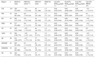
The UK-wide median (5th and 95th percentile) KGEmod[sqrt] is 0.94 (0.83, 0.97) for calibration (CP) and for evaluation 0.92 (0.80, 0.96) and 0.92 (0.78, 0.96) for P1 and P2, respectively (Table 2). Median PBIAS across all catchments over CP is low, −0.1 % (−3.7, 0.7 %). Overall, GR4J performs well against streamflow observations and parameter sets remain stable across P1 and P2 with comparable performance to Crochemore et al. (2017) and Poncelet et al. (2017) using GR6J for catchments across France, Germany, and Austria. For completeness and comparison with other works, the NSE was calculated as it is the most universally used metric. Spatial maps and summary statistics for KGEmod[sqrt] and NSE are provided in Fig. S1 in the Supplement and, notwithstanding differences in study design, results for GR4J are on par with other large sample catchment modelling studies in the UK (e.g. Crooks et al., 2009, using the probability distributed model (PDM; Moore, 2007) for 120 catchments). All streamflow simulations (proxy observations, and benchmark and ESP forecasts) were generated using model parameter sets calibrated over CP and with KGEmod[sqrt] as objective function; median and ranges of calibrated parameter values for GR4J X1, …, X4 across the UK and nine hydroclimate regions are given in Table 2 and for individual catchments in Table S1 along with respective performance metrics.
3.2 Generation of ESP hindcasts from historic climate data
In step 2, initial hydrologic conditions (IHCs) were estimated for each catchment and forecast initialization date by forcing the calibrated GR4J model with 4 years of observed P and ETp previous to the forecast initialization date, over the 1961–2015 period, thus the first usable forecast date after model spin up is 1 January 1965. Secondly, a 51-member ensemble m of streamflow hindcasts was generated for each forecast initialization date (first of each month) by forcing GR4J with 51 historic climate sequences (P and ETp pairs) extracted from 1961 to 2015 out to a 12-month lead time at a daily time step. Each of the 51 generated hindcast time series were then temporally aggregated to provide a forecast of mean streamflow over seamless lead times of 1 day to 12 months, resulting in 365 lead times per forecast (leap days were removed). Following convention in the HOUK, lead time (LT) in this paper refers to the streamflow (expressed as mean daily streamflow) over the period from the forecast initialization date to n days (or months) ahead in time. So a January ESP forecast with 1-month lead time is the mean daily streamflow from 1 January to the end of January and a January forecast with 2-month lead time is the mean daily streamflow from 1 January to the end of February.
Although it is not possible to create a hindcast experiment under exactly the same conditions experienced in operational mode, effort was made to ensure historic climate sequences did not artificially inflate skill (see Robertson et al., 2016) by using leave-three-years-out cross-validation (L3OCV) whereby the 12-month forecast window and the two succeeding years were not used as climate forcings. This was done to account for persistence from known large-scale climate–streamflow teleconnections such as the North Atlantic Oscillation with influences lasting from several seasons to years (Dunstone et al., 2016). Because this climate information could be an advantage, but is not available in operational forecasting, it was not used in the hindcast experiment. Using the first forecast on 1 January 1965 as an example, 51 sequences of P and ETp pairs of length 365 days (from 1 January to 31 December) were extracted from observed P and ETp records between 1961 and 2015, but not for 1965, 1966, or 1967. To keep a 51-member ensemble across all hindcast years, forecasts made in 2013 and 2014 did not have enough data for L3OCV so in these cases climate sequences from 1961, and 1961 and 1962, respectively, were instead removed. The skill of ESP was evaluated over a 50-year hindcast period N between 1965 and 2015 for each of 12 initialization months i (January to December) and all 365 LTs. In total, 600 hindcasts were generated (N×i) with 51 ensemble members each at 365 LTs across 314 catchments resulting in over 3.5 × 10⁹ forecast values of streamflow in the ESP hindcast archive.
3.3 Creation of proxy streamflow observation series
In step 3, a proxy streamflow observation series was produced by forcing the calibrated GR4J model with observed P and ETp over 1961–2015 with a 4-year model spin-up. A 4-year model spin up ensures model states are appropriately stabilized, especially important for slower responding catchments (e.g. in Southern England and Anglian regions). The proxy observation series, the best estimate of streamflow observations given current model and observed meteorological data, is used to evaluate ESP forecasts against. It is common to use this approach instead of using direct streamflow observations as it has the advantage of isolating loss of skill to IHCs rather than from model errors and biases (e.g. Alfieri et al., 2014; Pappenberger et al., 2015; Wood et al., 2016a; Yossef et al., 2013).
3.4 Evaluation of ESP skill
In step 4, forecast skill is presented as a skill score, which is the improvement over the benchmark forecast using some measure of accuracy A, given generically by Wilks (2011) in Eq. (1):
where Afc is the accuracy measure of the hydrological forecasting system Qfc (here ESP) against observations (here ∗proxy observations); Abench is the accuracy measure of the benchmark forecast Qbench against , and Aperf is the value of A in the case of a perfect forecast (typically 1 or 0 depending on metric). For each forecast made over the hindcast period the probabilistic skill of the full ESP 51-member ensemble forecast Qfc was evaluated against a probabilistic climatology benchmark forecast Qbench. Qbench was calculated as the full sample climatological distribution of proxy streamflow observations over 1965–2015 for the forecast period. Similar to the historic climate forcing sequences in Sect. 3.2, the probabilistic climatology benchmark forecast was also created using L3OCV to account for persistence known to occur for several years in streamflow, particularly during drought (Wilby et al., 2015). In testing, we performed the skill evaluation with and without cross-validation of ESP forecasts and streamflow climatology benchmark forecasts. It was found that cross-validation was important, as in some cases failing to cross-validate ESP forecasts inflated skill scores whereas failing to cross-validate climatological benchmark forecasts deflated skill scores (i.e. the benchmark forecast was advantaged thereby disadvantaging ESP forecasts); in some cases skill scores were advantaged/disadvantaged by ±15 %.
The continuous ranked probability score (CRPS) (Hersbach, 2000) accuracy measure A, and corresponding skill score (CRPSS), was used for evaluating the probabilistic skill of ESP. The CRPS penalizes biased forecasts and those with low sharpness (Wilks, 2011). The Ferro et al. (2008) ensemble size correction for CRPS was applied to account for differences between the number of members in Qfc (period 1961–2015 → L3OCV ) and Qbench (period 1965–2015 → L3OCV ), as done in evaluation of hydrological ensemble forecasting elsewhere (e.g. Crochemore et al., 2017). Calculation of skill scores was undertaken using the open source “easyVerification” package v0.4.2 in R (MeteoSwiss, 2017).
The CRPS is one of the most recommended scores for evaluation of overall hydrological ensemble forecast performance (Pappenberger et al., 2015). However, several commonly used metrics were also calculated for evaluation of deterministic ESP performance (using the ESP ensemble mean): Pearson correlation coefficient (Cor.), the mean squared error skill score (MSESS), and the deterministic equivalent to CRPSS, the mean absolute error skill score (MAESS). The pattern of results in terms of where and when ESP is most/least skilful was found to be independent of chosen metric, with virtually identical results between probabilistic (using CRPSS) and deterministic (using MAESS) results (see Fig. S2), and so for brevity the remainder of paper is based on CRPSS only. A skill score of 1 indicates a perfect forecast, a skill score > 0 shows the ESP forecast is more skilful than the benchmark, a skill score = 0 shows ESP is only as accurate as the benchmark, and a skill score < 0 warns that ESP is inferior to the benchmark forecast. The CRPSS was applied to the 314 catchments for the 12 initialization months and 365 lead times for each year over the 50-year hindcast period.
Results are presented in the following order: First, ESP skill is shown for all 365 lead times (LT), then by forecast initialization month for a sample of eight representative LTs commonly used in operational hydrological forecasting (i.e. short (1 and 3 days), extended (1 and 2 weeks), monthly (1 month), seasonal (3 and 6 months), and annual (12 months)). Second, the spatial distribution of ESP skill is shown, both averaged across the UK and each of the nine hydroclimate regions, then for individual catchments to explore sub-region heterogeneity. Third, the relationship between catchment storage and ESP skill is assessed.
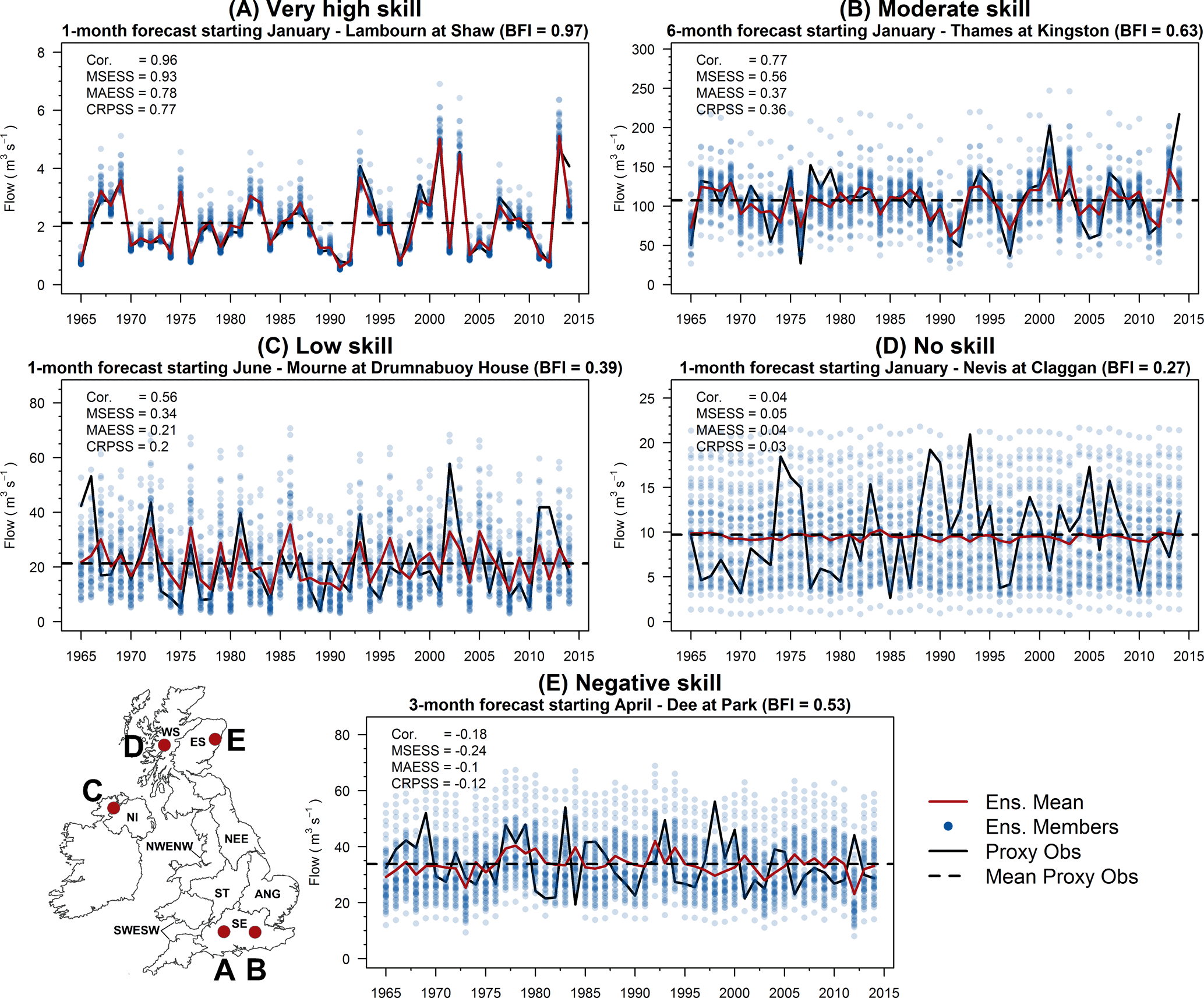
Figure 2Five example 1965–2015 hindcast time series in which skill metrics range from very high (a) to negative skill (e). The red line is the 51-member ESP ensemble mean, black line the proxy observed streamflow (also known as a perfect forecast), semi-transparent blue dots show the ensemble spread for each hindcast year, and the dashed horizontal black line shows mean proxy observed streamflow (analogous to a deterministic climatology benchmark forecast, although not cross-validated here as was done in calculation of skill scores (i.e. simply the same value repeated each year)).
Reducing accuracy of a forecast to a numeric skill metric value is abstract and difficult to interpret. Throughout the results and discussion sections skill score values are assigned qualitative descriptions according to degree of skill based on the CRPSS: very high [0.75, 1]; high [0.5, 0.75); moderate [0.25, 0.5); low (0, 0.25); no skill = 0, and negative skill < 0; CRPSS values which are near zero, defined between ±0.05, are regarded as “neutrally skilful” (after Bennett et al., 2017). Five example 1965–2015 hindcast time series with skills ranging from very high to negative skill are visualized in Fig. 2 and act as a graphical reference in the remainder of the paper to aid interpretation of skill.
4.1 Timing of ESP skill
4.1.1 Lead time
UK-wide mean ESP skill across all catchments and initialization months decays exponentially as a function of lead time (Fig. 3). Mean CRPSS values from short (1-day) to extended (2-week) lead times range from 0.75 to 0.30, and across monthly, seasonal (3-month), and annual lead times from 0.20, 0.11, to 0.04, respectively. There is large spread around mean skill scores for any lead time, depicted by the semi-transparent 5th and 95th percentile bands across the 314 catchments in Fig. 3. For example, at a 2-week lead time CRPSS values are bound between 0.11 and 0.71, and for monthly lead times between 0.06 and 0.59. Skill scores for the deterministic ESP ensemble mean (measured by MAESS) are virtually the same as those for probabilistic forecasts (measured by CRPSS) for all lead times and regions (see Fig. S2c and d).
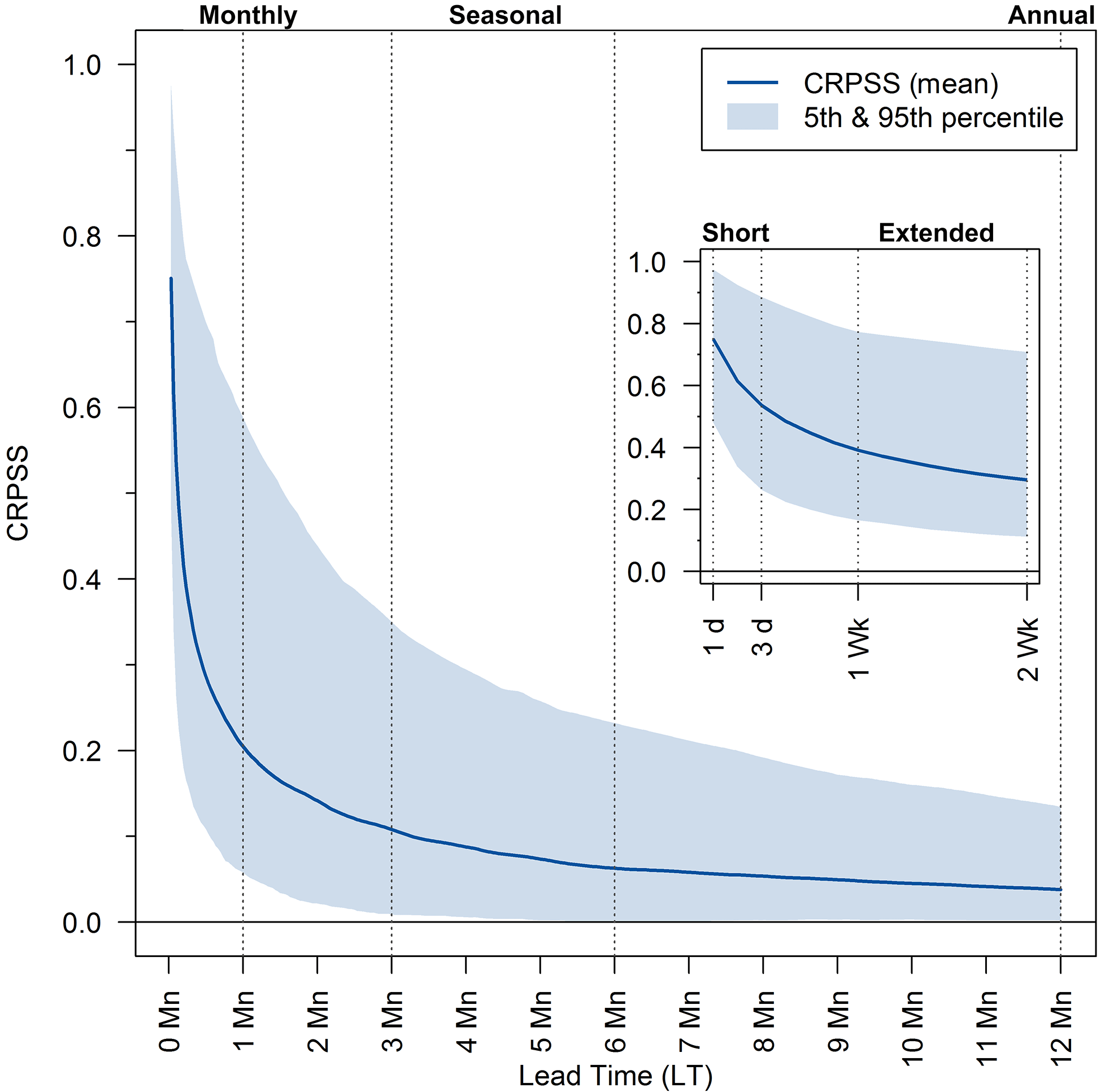
Figure 3UK-wide mean ESP CRPSS values across all 314 catchments and 12 forecast initialization months for all 365 lead times (LTs) with short and extended lead times also shown inset for readability. The range of skill scores across catchments at each LT is shown by the semi-transparent 5th and 95th percentile band. Vertical lines represent eight commonly used operational forecasting LTs from short (1 and 3 days), extended (1 and 2 weeks), monthly (1 month), seasonal (3 and 6 months), to annual (12 months).
4.1.2 Initialization month
ESP skill varies depending on forecast initialization month (IM) and the time of year, with highest and lowest skill conditional on lead time. Figure 4 shows skill scores for initialization months January to December for short and extended lead times (LTs) as summarized by boxplots across all catchments. Skill scores for these four sample LTs (1-day, 3-day, 1-week, and 2-week) are highest in summer months (June, July, and August) with August the most skilful forecast IM on average, whereas skill is lower for winter months (December, January, and February) with January the least skilful forecast IM. Skill scores across IMs for the four sample monthly to annual LTs are shown in Fig. 5. Skill is also highest for the 1-month forecasts when initialized in August, however for 3-month, 6-month, and 12-month LTs, forecast skill is generally higher for autumn (September, October, and November) and winter IMs, with October the most skilful on average. All four monthly, seasonal, and annual LTs have lowest skill scores when initialized in spring months, particularly April, which in the UK is a transition month between winter months with lowest soil moisture deficits (SMDs) and warmer summer months with highest SMDs.
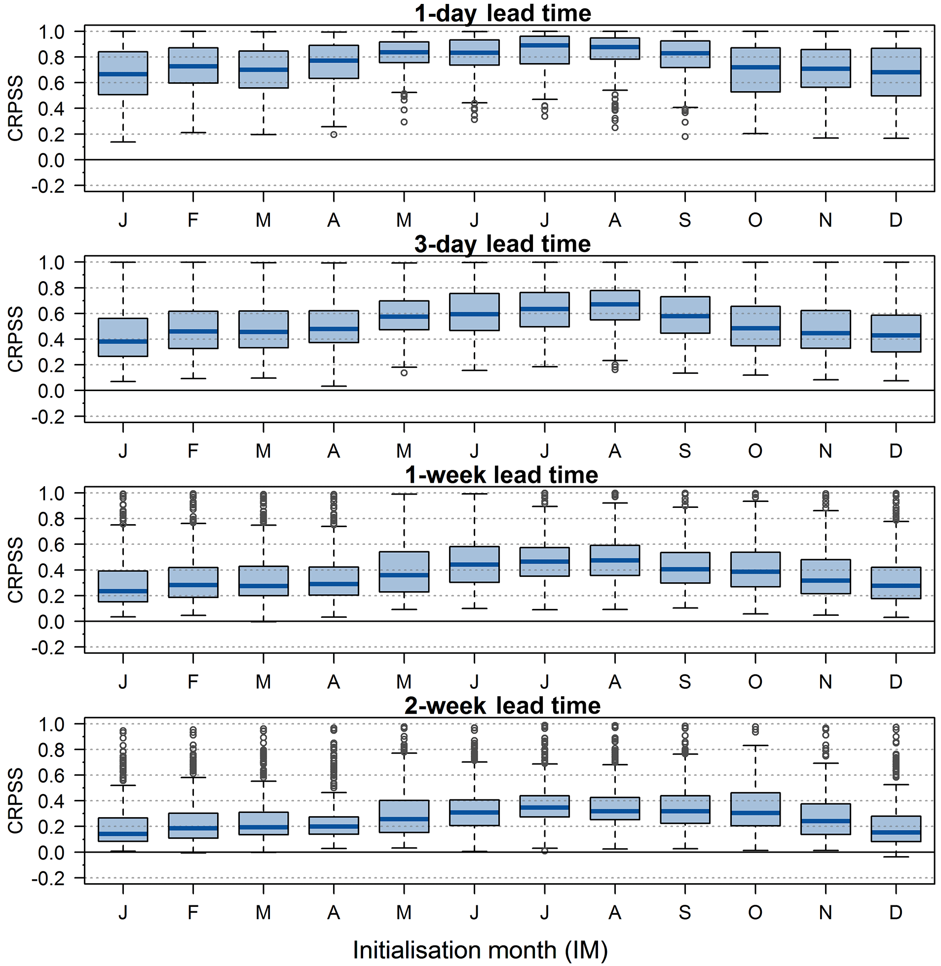
Figure 4UK-wide ESP skill scores across 314 catchments for each of the 12 forecast initialization months for four short and extended lead times. Boxplots summarize CRPSS values with the blue line representing the median, and boxes the interquartile range (IQR); whiskers extend to the most extreme data point, which is no more than 1.5 times the IQR from the box, and grey circles are outliers beyond this range.
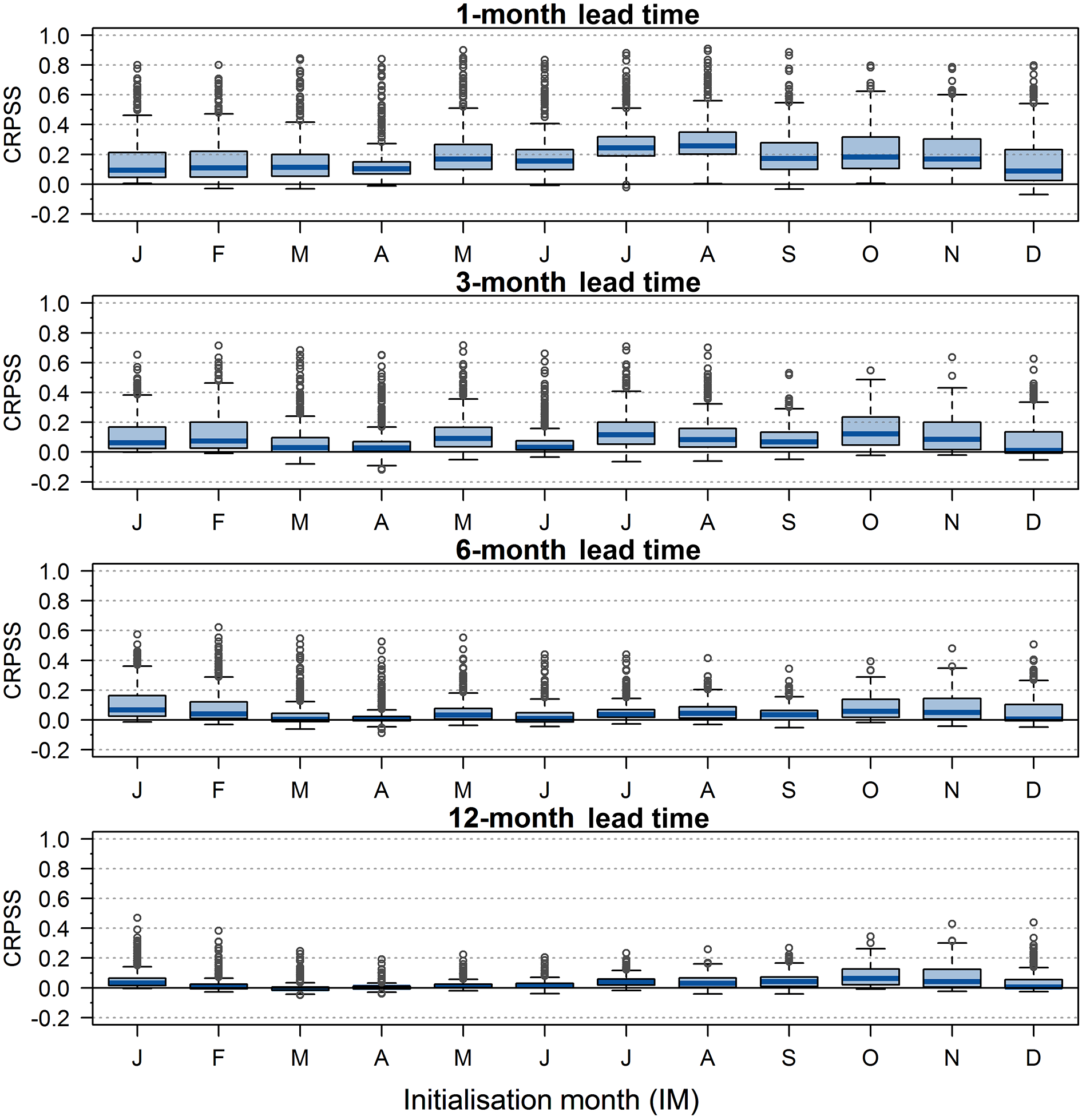
The decay in skill with LT as shown in Fig. 3 also occurs across all initialization months (Figs. 4 and 5). Whilst mean ESP skill tends towards zero for longer LTs, there are many catchments with much higher than average skill scores. For example, for 1-month LT ESP forecasts initialized in August the average UK-wide ESP skill is moderate (CRPSS = 0.30), but 36 catchments have high skill (CRPSS ≥ 0.5), and a CRPSS as high as 0.91 is achieved for the Lambourn at Shaw in Southern England.
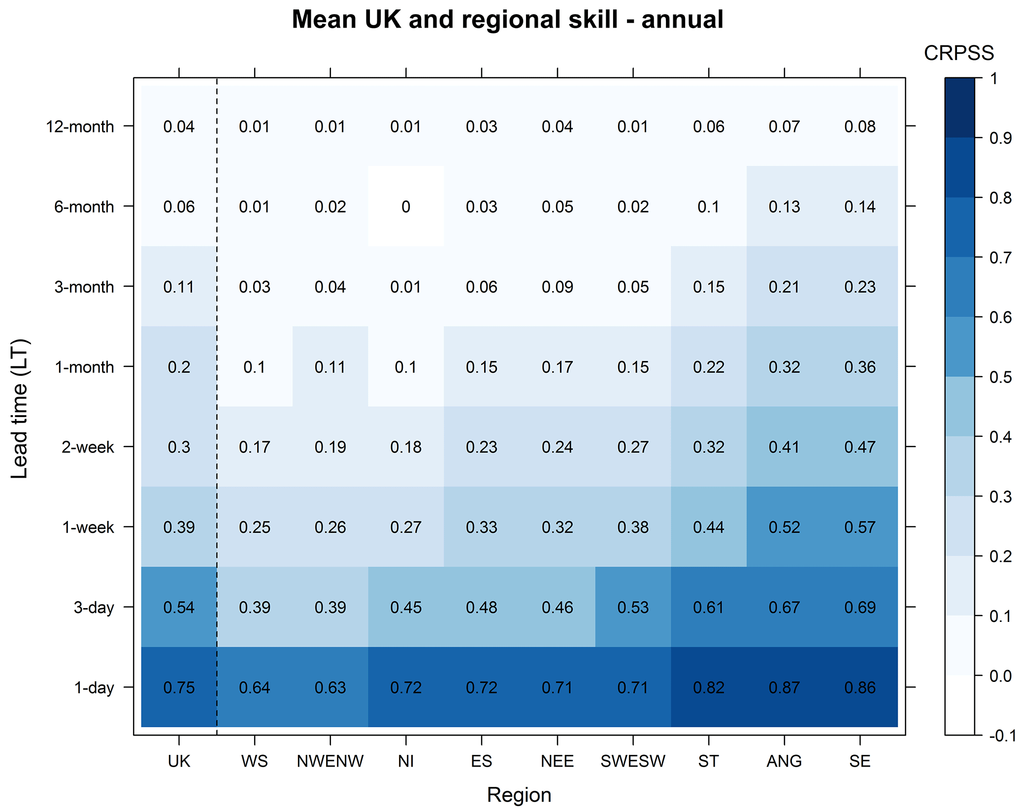
Figure 6Mean ESP skill across all 12 forecast initialization months for the UK and for each of the nine hydroclimate regions ordered from least to most skilful (horizontal axis) at eight sample lead times (vertical axis). Skill is given by the CRPSS with darker and lighter shades showing higher and lower skill, respectively; mean skill score values are shown within each cell.
4.2 Spatial distribution of ESP skill
4.2.1 UK hydroclimate regions
Figure 6 shows a heatmap of mean ESP skill across initialization months for the UK and for nine hydroclimate regions using the CRPSS metric. The same patterns are found for Cor., MSESS, and MAESS (Fig. S2). ESP skill has a prominent spatial pattern across the UK consistent over shorter and longer LTs. Least skilful UK regions are Western Scotland (WS), North-west England & North Wales (NWENW), and Northern Ireland (NI), whereas Severn-Trent (ST), Anglian (ANG), and Southern England (SE) are most skilful. Using a 1-week LT as an example, ESP is over twice as skilful in SE (CRPSS = 0.57) than in WS (CRPSS = 0.25). All regions are, on average, skilful out to 1-month LT, but by 3-month LT WS, NWENW, and NI are only neutrally skilful; at LTs up to 6 and 12 months ST, ANG, and SE are the only regions to remain skilful, as a whole.
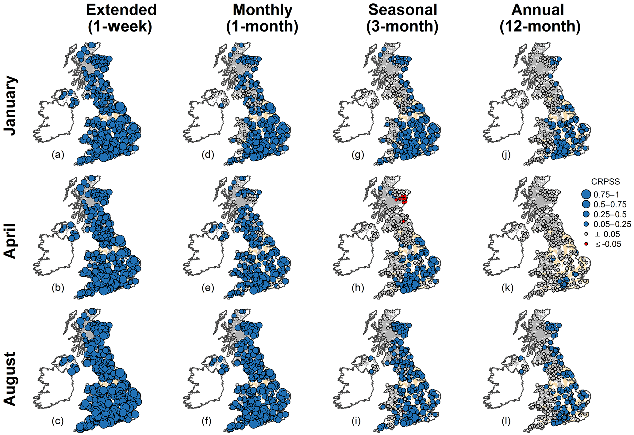
Figure 7ESP skill for individual forecasts made at each of the 314 catchment locations for four sample lead times (columns) and three initialization months (rows). Larger and smaller circles represent higher and lower skill from CRPSS, respectively, with blue circles when ESP is more skilful than benchmark climatology and red when ESP is less skilful. Grey circles represent neutrally skilful forecasts (i.e. CRPSS values between ±0.05).
4.2.2 Catchment scale
There is considerable sub-region heterogeneity when skill scores for individual forecasts at the catchment scale are examined. CRPSS values are mapped in Fig. 7 for all 314 catchment locations for a sample of four LTs (ranging from extended to annual) and three initialization months (January, April, and August). Although WS is considered a low skill region overall at a 1-week LT in Fig. 6 (i.e. CRPSS = 0.248), moderate to high skill ESP forecasts can be made for some catchments at different times of the year. For example, August 1-week LT forecasts (Fig. 7c) in WS are moderately skilful (CRPSS ≥ 0.25) for over 80 % of the 35 catchments or even highly skilful (CRPSS ≥ 0.5) for 20 % of catchments. In all regions, almost all individual catchments are more skilful than the benchmark climatological forecast for up to extended LTs (i.e. Fig. 7a–c).
Sub-region heterogeneity is much more apparent for monthly, seasonal, and annual LTs (Fig. 7d–l). As in Fig. 6, skill decays at different rates depending on region and lead time, but also initialization month. However, the finer spatial information in Fig. 7 shows that skill decays towards zero at vastly different rates for individual catchments even within the same region. For example, despite low average skill of January 12-month LT forecasts in SE (CRPSS = 0.14), nearly 20 % of catchments have moderate skill. In April, when UK-wide forecasts at longer LTs are least skilful (i.e. Fig. 5), skilful forecasts can still be made at monthly and seasonal LTs for the majority of catchments in ST, ANG, and SE (Fig. 7e and h). Sub-region heterogeneity is perhaps most prominent for the Thames basin in SE. The April 3-month LT forecast for the Thames at Kingston has low skill (CRPSS = 0.22, size = 9948 km2), but two of its sub-catchments have contrasting skills; the Lambourn at Shaw is highly skilful (CRPSS = 0.65, size = 234 km2) whereas the forecast made for the Mole at Kinnersley Manor has effectively no skill (CRPSS = 0.02, size = 142 km2).
4.3 Relationship between catchment storage and ESP skill
The relationship between the two calibrated GR4J catchment storage parameters, X1 (soil moisture store capacity [mm]) and X3 (groundwater store capacity [mm]), BFI, and ESP skill (CRPSS) for n= 314 individual catchments is shown in the scatterplot matrix in Fig. 8 using the non-parametric Spearman's rank correlation coefficient ρ. It is difficult to link X1 and X3 specifically to soil moisture and groundwater storage capacity, respectively, as GR4J is not a physically based hydrological model. However, their sum (X1 + X3) can be considered an estimate of total catchment storage (excluding water in the river channel and snowpack). Total catchment storage (X1 + X3) is strongly positively (non-linearly) correlated with BFI (ρ= 0.87); catchments with high BFIs tend to have much higher than average catchment storage capacity. The BFI is also very strongly positively correlated with ESP skill (ρ= 0.90). The 1-month LT forecast skill (based on CRPSS) averaged across all 12 initialization months is used to demonstrate this, but similar results are found over the range of lead times, individual initialization months, and skill metrics (not shown). Forecasts in the most responsive catchments (BFI ≤ 0.35, 20 % of catchments) have on average low skill (CRPSS = 0.08) whereas the slowest responding catchments (BFI ≥ 0.9, 5 % of catchments) have high skill (CRPSS = 0.66).
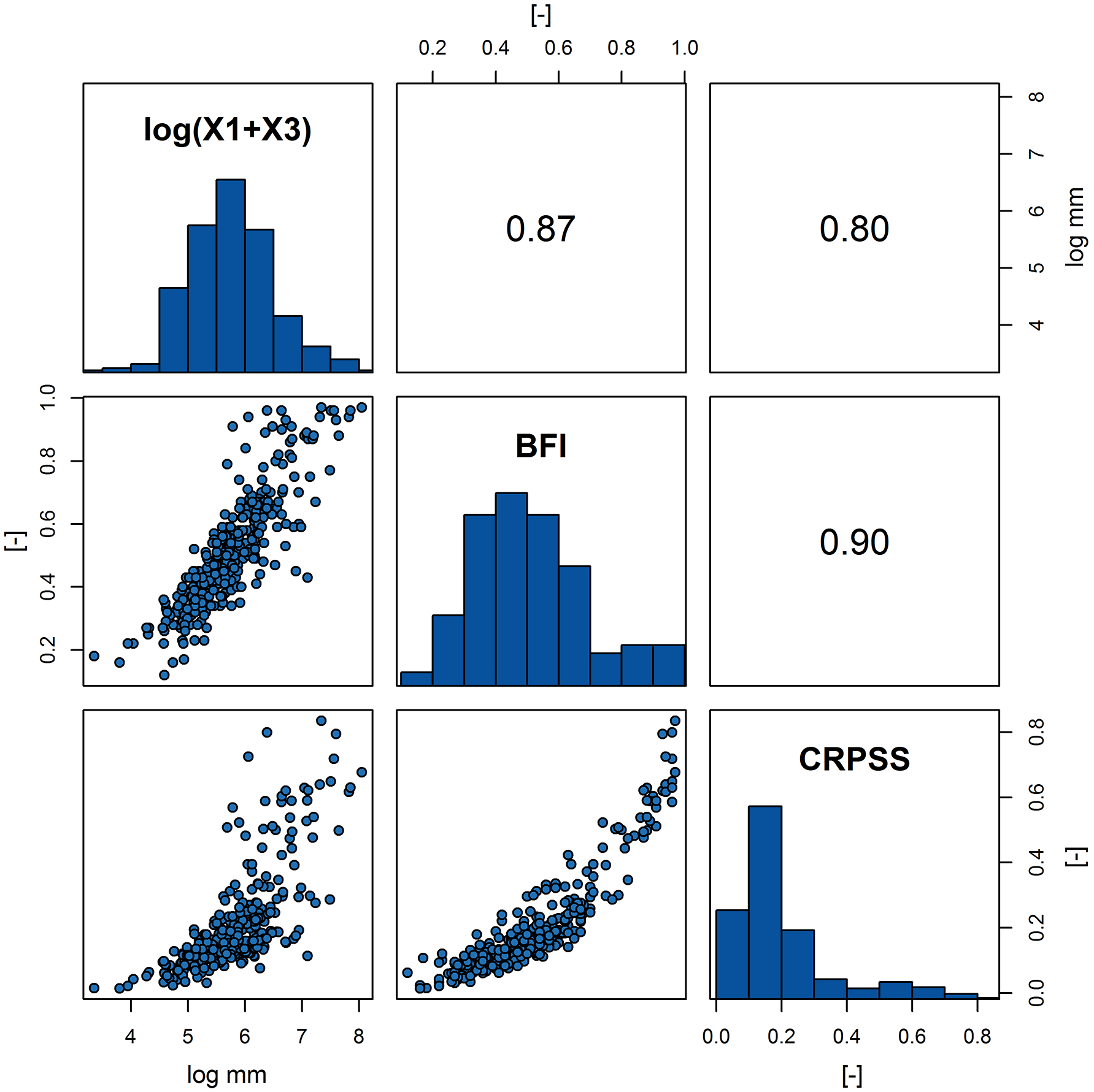
Figure 8Scatterplot matrix between catchment storage capacity (X1 soil moisture store capacity [mm] + X3 groundwater store capacity [mm]), BFI, and ESP skill (CRPSS) with n= 314 using the non-parametric Spearman's rank correlation coefficient ρ. Skill is the 1-month CRPSS skill score magnitude averaged across all 12 initialization months. Catchment storage capacity (X1 + X3) was re-expressed by taking the natural log, as raw values are heavily positively skewed.
Overall, the ESP method is found to be skilful when benchmarked against climatology in the UK, but the degree of skill is dependent on lead time, initialization month, and individual catchment location and storage properties.
5.1 When is ESP skilful?
UK-wide ESP forecasts for short lead times (out to 3 days) are on average highly skilful (CRPSS ≥ 0.5) and for extended lead times (out to 2 weeks) moderately skilful (CRPSS ≥ 0.25). Mean ESP skill decays exponentially with increasing lead time so skill is on average much lower for monthly, seasonal, and annual lead times, as expected. However, the magnitude of skill is not uniform across the 12 forecast initialization months. ESP skill for short, extended, and monthly lead times is higher than average when initialized in summer months and lower than average for winter months. Svensson (2016) also found higher skill across the UK when initialized in summer (highest also for August forecasts at a 1-month lead time) using the statistical persistence forecasting method. This is consistent with Li et al. (2009) and Shukla and Lettenmaier (2011), who found soil moisture initial hydrologic conditions (IHCs) contributed to greater skill for forecasts initialized in the warmer summer season than the cold winter season in the south-east of the US, up to a 1-month lead time; this was said to be due to drier initial soil moisture states in summertime. Similarly, Staudinger and Seibert (2014) found drier initial soil moisture was connected to longer persistence in all seasons except winter in Switzerland. Soil moisture deficits (SMDs) are also highest in summer in the UK, peaking in July, and lowest in winter (based on UK Met Office MORECS dataset (Hough and Jones, 1997) over 1961–2015). This could help explain why up to 1-month LT hydrological forecasts initialized in summer months using IHCs alone (e.g. ESP) are more skilful than if initialized in winter in the UK. Higher summer ESP forecast skill could be capitalized upon operationally given seasonal climate predictability over northern Europe is notoriously challenging for summer rainfall (e.g. Weisheimer and Palmer, 2014).
In contrast, ESP skill at seasonal to annual lead times is generally higher than average when initialized in winter and autumn months, and lowest in April. However, these higher skills occur in catchments with higher BFIs, suggesting that perhaps groundwater from large slowly responding aquifers is the source of ESP skill at these longer lead times. This is supported by Wood and Lettenmaier (2008), who found that baseflow dominates hydrological persistence in winter in the Rio Grande River in the US. Staudinger and Seibert (2014) also found for simulations initialized in winter, wetter initial conditions lead to longer persistence, although they note it was difficult to separate the relative influences from snow and aquifer memory. Lower longer-range skill for forecasts initialized in spring months was also found by Svensson (2016) for a 3-month LT based on statistical streamflow persistence forecasts. However, there are limited seasonal hydrological hindcast studies for the UK that have also assessed skill at longer than 3-month lead times to compare results. Spring in the UK is characterized as a transition season between lowest (winter) and highest (summer) SMDs, in which groundwater recharge no longer occurs and baseflow begins its recession. Factors that might contribute to lower skilled forecasts initialized in spring, and indeed to differences in skill across all initialization months, include: potentially higher variability in IHC storage states, changing variability in rainfall across the forecast window (e.g. from late spring to early autumn), and differences in model performance for different months over the year due to the global calibration of GR4J. Given the answer is likely a combination of many of these factors, among others, further work should endeavour to attribute differences in skill during different times of the year, but this is outside the scope of this paper.
5.2 Where is ESP skilful?
The skill of ESP is also not uniformly distributed in space. Least skilful hydroclimate regions within the UK are situated in the north and west (WS, NWENW, and NI) whereas the most skilful are situated in the south and east (ST, ANG, and SE) across all lead times studied. This prominent spatial pattern was also noted, among others, by Svensson et al. (2015) and Svensson (2016) using statistical persistence forecasting and Bell et al. (2017) using a gridded national-scale hydrological model. These space–time patterns are also apparent in skill maps of individual catchments (i.e. Fig. 7), although there is marked sub-region heterogeneity, as demonstrated using the Thames basin: the slow responding Lambourn at Shaw sub-basin (BFI = 0.97) was highly skilful whereas the fast responding Mole at Kinnersley Manor catchment (BFI = 0.39) had virtually no ESP skill.
5.3 Why is ESP skilful?
The most skilful ESP regions of the UK are also those that are underlain by the UK's principal aquifers (Fig. 1). Catchments with larger calibrated soil moisture and groundwater storage capacity parameters in GR4J (i.e. X1 and X3) are also situated in ST, ANG, and SE, and tend to have a higher base flow index (BFI) (Table 2). The BFI is therefore broadly interpreted here as an integrated index of catchment storage capacity and is inferred to be responsible for modulating ESP skill – catchments with higher storage are more skilful with skill decaying at a much slower rate as lead time increases, compared to catchments with low storage capacity. For example, forecasts for the Lambourn remains on average moderately skilful (i.e. CRPSS ≥ 0.25) until a lead time of 306 days, but the Mole drops below the moderately skilful threshold at a lead time of just 10 days.
These findings are consistent with the current physical understanding of sources of ESP skill in non-snow dominated catchments in the literature. Water storage within the soil introduces a memory effect whereby anomalously dry or wet conditions can take weeks or months to be “forgotten” (Ghannam et al., 2016; Li et al., 2009), and the slow transformation of precipitation to streamflow in catchments with highly permeable aquifers in the south east of the UK leads to temporal streamflow dependence for up to a season ahead, and longer (Chiverton et al., 2015). Although it is encouraging that GR4J storage parameter values (X1 and X3) appear to show some physical realism, a note of caution is needed as GR4J is not a physically based hydrological model, nor is it guaranteed that these results are directly transferable to any lumped catchment hydrological model. It has also been noted that the BFI in the UK is influenced by many other factors such as lake and snow storage (Parry et al., 2016), therefore a more detailed examination of the physical hydrogeological controls on catchment BFI, such as in Bloomfield et al. (2009) for the Thames, is needed at a national scale.
The ESP method was originally developed and tested in the snow dominated catchments of the western US with particular strength in forecasting spring snow melt driven streamflow (e.g. Franz et al., 2003; Wood and Lettenmaier, 2008). Because the source of ESP is from IHCs, and because individual catchments will have different relative contributions of IHC sources (e.g. snow, soil moisture, and groundwater), ESP skill must be assessed using a large sample of diverse catchment types and sizes for each region it is being applied in (e.g. Yossef et al., 2013). The present study adds to the broader international literature on benchmarking ESP skill in non-snow dominated catchments. In particular, results show that IHCs in catchments with large soil moisture and groundwater storage provide skill up to a year ahead. It must however be acknowledged that the UK is not completely snow-free. Just under 5 % of catchments studied have a significant snow contribution (i.e. > 0.15) located mainly in upland areas of Eastern Scotland (ES) (see Fig. 1). In the present experimental set-up, snow accumulation and melt processes were not represented within the GR4J model. This would explain why ES has the lowest GR4J model performance for the reference simulation of all regions (Table 2). In addition, the worst performing forecast in the entire ESP hindcast archive is the 3-month LT April forecast for the Dee at Park with a negative CRPSS = −0.12 (see Fig. 2e). In this instance both the ESP forecast and the proxy streamflow observations (or perfect model) which the forecast was evaluated against was not a good enough representation of reality.
ESP in its traditional form as used here provides the lower limit of streamflow forecasting skill in the absence of skilful atmospheric forecasts (Pagano et al., 2010) or improved hydrological process representation (e.g. snow). As such, ESP assumes near total uncertainty about future rainfall; when there is limited to no influence of IHCs on streamflow prediction (e.g. highly responsive catchments), the ESP ensemble mean and spread defaults to climatology (see Fig. 2d). Given the known influence of the NAO on rainfall and therefore streamflow in the UK, particularly in the north and west for winter (e.g. Svensson et al., 2015), there is potential for an NAO-conditioned ESP method to be developed. This would involve sub-sampling historic climate sequences used to force ESP based on years most similar to NAO conditions at the time of forecast. Beckers et al. (2016) developed an ENSO-conditioned ESP method for three test sites in the US Pacific Northwest and found skill improvements in the order of 5–10 %; the study also presented the added value of including a weather resampling technique to account for the unavoidable reduction in ensemble size. Overall, low ESP forecast performance and sharpness in highly responsive catchments in the north and west would be expected to improve with the incorporation of information that reduces rainfall forcing uncertainty at all lead times but particularly seasonal, whether from ensemble sub-sampling or inclusion of skilful atmospheric forecasts.
Ensemble streamflow prediction (ESP) has a rich history internationally as a low cost and efficient ensemble hydrological forecasting system used operationally across a range of lead times. The ESP method using simple lumped conceptual hydrological models is currently one of three methods used within the operational Hydrological Outlook UK (HOUK) seasonal hydrological forecasting service and also feeds into the Environment Agency's monthly “Water Situation Report for England”. However, the skill of ESP at the catchment scale under a rigorous hindcast experiment for a large sample of diverse catchments across the UK had not previously been investigated.
We conclude that ESP is skilful against a climatology benchmark forecast in the majority of catchments across all lead times up to a year ahead, but the degree of skill is strongly conditional on lead time, forecast initialization month, and individual catchment location and storage properties. In summary:
-
ESP skill decayed exponentially with increasing lead time but catchments with larger storage capacity decayed at a much slower rate, resulting in the possibility of low to moderate skill forecasts based on initial hydrologic conditions (IHCs) alone even at a 12-month lead time for some catchments.
-
For short (1–3 days), extended (1–2 weeks), and monthly forecasts, skill was highest when initialized in summer months and lowest in winter months.
-
For seasonal (3–6 months) to annual forecasts, skill was highest when initialized in winter and autumn months, but only for catchments with high storage capacity (i.e. high base flow index). Longer range forecast skill was lowest when initialized in spring, particularly April, which is likely due to the complex interplay of hydrological and climatological processes involved during the transition from lower winter to higher summer soil moisture deficit conditions and needs to be explored further.
-
ESP is most skilful in the south and east of the UK, where slower responding catchments with higher storage are mainly located. This is in contrast to the more highly responsive catchments in the north and west which are generally not skilful at seasonal lead times. However, substantial sub-region heterogeneity was observed and skilful ESP forecasts are still possible at the individual catchment scale despite when the region as a whole has low skill.
We show that simple lumped conceptual rainfall-runoff models (here using GR4J) are able to be used to produce skilful ESP forecasts at short to annual lead times in the UK. This hindcast experiment provides scientific justification for when (lead time and initialization month) and where (region and catchment types) use of such a relatively simple forecasting approach is appropriate. Currently, ESP is only used operationally in the UK at seasonal and annual lead times in England and Wales. This skill evaluation has shown that much higher skills are possible for short (1–3 days) and extended (1–2 weeks) lead times in all regions across the UK and opens the potential for applying ESP as a low cost and efficient catchment-scale ensemble hydrological forecasting system in a wider context.
Finally, most ensemble hydrological forecasting systems are benchmarked against an arguably too simplistic climatology benchmark forecast which is not particularly challenging to beat. Pappenberger et al. (2015) calls this “naïve skill” and argues that a forecasting system can only be classified as having “real skill” when it performs better than a “tough to beat” lower cost benchmark forecast system. The ESP hindcast archive derived and presented in this study provides such a “tough to beat” simplified hydrology model benchmark in which the potential value of improvements from more sophisticated forms of ESP (e.g. incorporation of snow processes, sub-sampling historic climate) or more complex and expensive hydro-meteorological ensemble forecasting systems can be judged. When and where ESP cannot provide skilful streamflow forecasts provides an opportunity to benchmark the degree to which recent improvements in seasonal prediction of UK regional rainfall (e.g. Baker et al., 2017) leads to improvements over using IHCs alone (i.e. our ESP method), and is the focus of future work.
The ESP hindcast archive (∼ 60 GB) and the “UK Hydroclimate Regions” shapefile can be requested from the Centre for Ecology & Hydrology (CEH), Wallingford, UK. Supplement Table S1 includes metadata for all 314 catchments as well as data used to generate Table 1 and 2, and Fig. 8 for others to explore.
The supplement related to this article is available online at: https://doi.org/10.5194/hess-22-2023-2018-supplement.
The authors declare that they have no conflict of interest.
This article is part of the special issue “Sub-seasonal to seasonal hydrological forecasting”. It is not associated with a conference.
This work was funded by NERC National Capability funding to CEH and the NERC
funded Improving Predictions of Drought for User Decision-Making (IMPETUS)
project (NE/L010267/1). Statistical analyses and graphics were implemented in
the open-source R programming language. Streamflow data and metadata are from
the NRFA and MORECS dataset from the UK Met Office. We thank Cecilia Svensson
for fruitful discussions about this work and Nuria Bachiller-Jareno for help
in designation of the UK Hydroclimate Regions. Finally, we thank Guillaume
Thirel and two anonymous referees for their constructive feedback that has
greatly improved this paper.
Edited by:
Quan J. Wang
Reviewed by: Guillaume Thirel and two anonymous
referees
Alfieri, L., Pappenberger, F., Wetterhall, F., Haiden, T., Richardson, D., and Salamon, P.: Evaluation of ensemble streamflow predictions in Europe, J. Hydrol., 517, 913–922, https://doi.org/10.1016/j.jhydrol.2014.06.035, 2014.
Anghileri, D., Voisin, N., Castelletti, A., Pianosi, F., Nijssen, B., and Lettenmaier, D. P.: Value of long-term streamflow forecasts to reservoir operations for water supply in snow-dominated river catchments, Water Resour. Res., 52, 4209–4225, https://doi.org/10.1002/2015WR017864, 2016.
Arnal, L., Cloke, H. L., Stephens, E., Wetterhall, F., Prudhomme, C., Neumann, J., Krzeminski, B., and Pappenberger, F.: Skilful seasonal forecasts of streamflow over Europe?, Hydrol. Earth Syst. Sci. Discuss., https://doi.org/10.5194/hess-2017-610, in review, 2017.
Baker, L. H., Shaffrey, L. C., and Scaife, A. A.: Improved seasonal prediction of UK regional precipitation using atmospheric circulation, Int. J. Climatol., https://doi.org/10.1002/joc.5382, 2017.
Beckers, J. V. L., Weerts, A. H., Tijdeman, E., and Welles, E.: ENSO-conditioned weather resampling method for seasonal ensemble streamflow prediction, Hydrol. Earth Syst. Sci., 20, 3277–3287, https://doi.org/10.5194/hess-20-3277-2016, 2016.
Bell, V. A., Davies, H. N., Kay, A. L., Brookshaw, A., and Scaife, A. A.: A national-scale seasonal hydrological forecast system: development and evaluation over Britain, Hydrol. Earth Syst. Sci., 21, 4681–4691, https://doi.org/10.5194/hess-21-4681-2017, 2017.
Bennett, J. C., Wang, Q. J., Robertson, D. E., Schepen, A., Li, M., and Michael, K.: Assessment of an ensemble seasonal streamflow forecasting system for Australia, Hydrol. Earth Syst. Sci., 21, 6007–6030, https://doi.org/10.5194/hess-21-6007-2017, 2017.
Berghuijs, W. R., Woods, R. A., and Hrachowitz, M.: A precipitation shift from snow towards rain leads to a decrease in streamflow, Nat. Clim. Change, 4, 583–586, https://doi.org/10.1038/nclimate2246, 2014.
Bloomfield, J. P., Allen, D. J., and Griffiths, K. J.: Examining geological controls on baseflow index (BFI) using regression analysis: An illustration from the Thames Basin, UK, J. Hydrol., 373, 164–176, https://doi.org/10.1016/j.jhydrol.2009.04.025, 2009.
Broderick, C., Matthews, T., Wilby, R. L., Bastola, S., and Murphy, C.: Transferability of hydrological models and ensemble averaging methods between contrasting climatic periods, Water Resour. Res., 52, 8343–8373, https://doi.org/10.1002/2016WR018850, 2016.
Chiverton, A., Hannaford, J., Holman, I., Corstanje, R., Prudhomme, C., Bloomfield, J., and Hess, T. M.: Which catchment characteristics control the temporal dependence structure of daily river flows?, Hydrol. Process., 29, 1353–1369, https://doi.org/10.1002/hyp.10252, 2015.
Coron, L., Perrin, C., and Michel, C.: airGR: Suite of GR hydrological models for precipitation-runoff modelling, R package version 1.0.2, available at: https://webgr.irstea.fr/airGR/?lang=en (last access: 14 July 2017), 2016.
Coron, L., Thirel, G., Delaigue, O., Perrin, C., and Andréassian, V.: The suite of lumped GR hydrological models in an R package, Environ. Model. Softw., 94, 166–171, https://doi.org/10.1016/j.envsoft.2017.05.002, 2017.
Crochemore, L., Ramos, M.-H., Pappenberger, F., and Perrin, C.: Seasonal streamflow forecasting by conditioning climatology with precipitation indices, Hydrol. Earth Syst. Sci., 21, 1573–1591, https://doi.org/10.5194/hess-21-1573-2017, 2017.
Crooks, S. M., Kay, A. L., and Reynard, N. S.: Regionalised Impacts of Climate Change on Flood Flows: Hydrological Models, Catchments and Calibration, Centre for Ecology & Hydrology, Environment Agency, Defra, London, 2009.
Day, G. N.: Extended Streamflow Forecasting Using NWSRFS, J. Water Resour. Plan. Manag., 111, 642–654, 1985.
Dunstone, N., Smith, D., Scaife, A., Hermanson, L., Eade, R., Robinson, N., Andrews, M., and Knight, J.: Skilful predictions of the winter North Atlantic Oscillation one year ahead, Nat. Geosci., 9, 809, https://doi.org/10.1038/ngeo2824, 2016.
Ferro, C. A. T., Richardson, D. S., and Weigel, A. P.: On the effect of ensemble size on the discrete and continuous ranked probability scores, Meteorol. Appl., 15, 19–24, https://doi.org/10.1002/met.45, 2008.
Franz, K. J., Hartmann, H. C., Sorooshian, S., and Bales, R.: Verification of National Weather Service Ensemble Streamflow Predictions for Water Supply Forecasting in the Colorado River Basin, J. Hydrometeorol., 4, 1105–1118, https://doi.org/10.1175/1525-7541(2003)004<1105:VONWSE>2.0.CO;2, 2003.
Ghannam, K., Nakai, T., Paschalis, A., Oishi, C. A., Kotani, A., Igarashi, Y., Kumagai, T., and Katul, G. G.: Persistence and memory timescales in root-zone soil moisture dynamics, Water Resour. Res., 52, 1427–1445, https://doi.org/10.1002/2015WR017983, 2016.
Gupta, H. V., Sorooshian, S., and Yapo, P. O.: Status of Automatic Calibration for Hydrologic Models: Comparison with Multilevel Expert Calibration, J. Hydrol. Eng., 4, 135–143, https://doi.org/10.1061/(ASCE)1084-0699(1999)4:2(135), 1999.
Gupta, H. V., Kling, H., Yilmaz, K. K., and Martinez, G. F.: Decomposition of the mean squared error and NSE performance criteria: Implications for improving hydrological modelling, J. Hydrol., 377, 80–91, https://doi.org/10.1016/j.jhydrol.2009.08.003, 2009.
Gustard, A., Bullock, A., and Dixon, J. M.: Low flow estimation in the United Kingdom, Institute of Hydrology, Wallingford, available at: http://nora.nerc.ac.uk/6050/ (last access: 3 November 2016), 1992.
Hamlet, A. F., Huppert, D., and Lettenmaier, D. P.: Economic Value of Long-Lead Streamflow Forecasts for Columbia River Hydropower, J. Water Resour. Plan. Manag., 128, 91–101, https://doi.org/10.1061/(ASCE)0733-9496(2002)128:2(91), 2002.
Harrigan, S., Hannaford, J., Muchan, K., and Marsh, T. J.: Designation and trend analysis of the updated UK Benchmark Network of river flow stations: The UKBN2 dataset, Hydrol. Res., https://doi.org/10.2166/nh.2017.058, 2017.
Hersbach, H.: Decomposition of the Continuous Ranked Probability Score for Ensemble Prediction Systems, Weather Forecast., 15, 559–570, https://doi.org/10.1175/1520-0434(2000)015<0559:DOTCRP>2.0.CO;2, 2000.
Hough, M. N. and Jones, R. J. A.: The United Kingdom Meteorological Office rainfall and evaporation calculation system: MORECS version 2.0 – an overview, Hydrol. Earth Syst. Sci., 1, 227–239, https://doi.org/10.5194/hess-1-227-1997, 1997.
Jolliffe, I. T. and Stephenson, D. B.: Forecast verification: a practitioner's guide in atmospheric science, John Wiley & Sons, England, 2003.
Keller, V. D. J., Tanguy, M., Prosdocimi, I., Terry, J. A., Hitt, O., Cole, S. J., Fry, M., Morris, D. G., and Dixon, H.: CEH-GEAR: 1 km resolution daily and monthly areal rainfall estimates for the UK for hydrological and other applications, Earth Syst. Sci. Data, 7, 143–155, https://doi.org/10.5194/essd-7-143-2015, 2015.
Klemeš, V.: Operational testing of hydrological simulation models, Hydrol. Sci. J., 31, 13–24, https://doi.org/10.1080/02626668609491024, 1986.
Kling, H., Fuchs, M., and Paulin, M.: Runoff conditions in the upper Danube basin under an ensemble of climate change scenarios, J. Hydrol., 424–425, 264–277, https://doi.org/10.1016/j.jhydrol.2012.01.011, 2012.
Letcher, R. A., Chiew, F. H. S., and Jakeman, A. J.: An Assessment of the Value of Seasonal Forecasts in Australian Farming Systems, Int. Congr. Environ. Model. Softw., available at: http://scholarsarchive.byu.edu/iemssconference/2004/all/79 (last access: 2 February 2017), 2004.
Li, H., Luo, L., Wood, E. F., and Schaake, J.: The role of initial conditions and forcing uncertainties in seasonal hydrologic forecasting, J. Geophys. Res.-Atmos., 114, D04114, https://doi.org/10.1029/2008JD010969, 2009.
MeteoSwiss: easyVerification: Ensemble Forecast Verification for Large Data Sets, R package version 0.4.2, available at: http://CRAN.R-project.org/package=easyVerification, last access: 14 July 2017.
Moore, R. J.: The PDM rainfall-runoff model, Hydrol. Earth Syst. Sci., 11, 483–499, https://doi.org/10.5194/hess-11-483-2007, 2007.
Nash, J. E. and Sutcliffe, J. V.: River flow forecasting through conceptual models part I – A discussion of principles, J. Hydrol., 10, 282–290, https://doi.org/10.1016/0022-1694(70)90255-6, 1970.
National Hydrological Monitoring Programme: Hydrological summary for the United Kingdom: April 2017, NERC/Centre for Ecology & Hydrology, Wallingford, UK, available at: http://nrfa.ceh.ac.uk/monthly-hydrological-summary-uk, last access: 20 May 2017.
National River Flow Archive: Integrated Hydrological Units of the United Kingdom: Hydrometric Areas with Coastline, available at: https://doi.org/10.5285/1957166d-7523-44f4-b279-aa5314163237 (last access: 10 June 2017), 2014.
Pagano, T., Hapuarachchi, P., and Wang, Q. J.: Continuous rainfall-runoff model comparison and short-term daily streamflow forecast skill evaluation, CSIRO, available at: https://publications.csiro.au/rpr/pub?pid=csiro:EP103545 (last access: 1 July 2017), 2010.
Pappenberger, F., Ramos, M. H., Cloke, H. L., Wetterhall, F., Alfieri, L., Bogner, K., Mueller, A., and Salamon, P.: How do I know if my forecasts are better? Using benchmarks in hydrological ensemble prediction, J. Hydrol., 522, 697–713, https://doi.org/10.1016/j.jhydrol.2015.01.024, 2015.
Parry, S., Wilby, R. L., Prudhomme, C., and Wood, P. J.: A systematic assessment of drought termination in the United Kingdom, Hydrol. Earth Syst. Sci., 20, 4265–4281, https://doi.org/10.5194/hess-20-4265-2016, 2016.
Perrin, C., Michel, C., and Andréassian, V.: Improvement of a parsimonious model for streamflow simulation, J. Hydrol., 279, 275–289, https://doi.org/10.1016/S0022-1694(03)00225-7, 2003.
Poncelet, C., Merz, R., Merz, B., Parajka, J., Oudin, L., Andréassian, V., and Perrin, C.: Process-based interpretation of conceptual hydrological model performance using a multinational catchment set, Water Resour. Res., 53, 7247–7268, https://doi.org/10.1002/2016WR019991, 2017.
Prudhomme, C., Hannaford, J., Harrigan, S., Boorman, D., Knight, J., Bell, V., Jackson, C., Svensson, C., Parry, S., Bachiller-Jareno, N., Davies, H., Davis, R., Mackay, J., McKenzie, A., Rudd, A., Smith, K., Bloomfield, J., Ward, R., and Jenkins, A.: Hydrological Outlook UK: an operational streamflow and groundwater level forecasting system at monthly to seasonal time scales, Hydrol. Sci. J., 62, 2753–2768, https://doi.org/10.1080/02626667.2017.1395032, 2017.
Robertson, D., Bennett, J., and Schepen, A.: How good is my forecasting method? Some thoughts on forecast evaluation using cross-validation based on Australian experiences, HEPEX Blog, available at: https://hepex.irstea.fr/how-good-is-my-forecasting (last access: 13 March 2017), 2016.
Robinson, E. L., Blyth, E., Clark, D. B., Comyn-Platt, E., Finch, J., and Rudd, A. C.: Climate hydrology and ecology research support system potential evapotranspiration dataset for Great Britain (1961–2015) [CHESS-PE], https://doi.org/10.5285/8baf805d-39ce-4dac-b224-c926ada353b7, 2016.
Robinson, E. L., Blyth, E. M., Clark, D. B., Finch, J., and Rudd, A. C.: Trends in atmospheric evaporative demand in Great Britain using high-resolution meteorological data, Hydrol. Earth Syst. Sci., 21, 1189–1224, https://doi.org/10.5194/hess-21-1189-2017, 2017.
Shukla, S. and Lettenmaier, D. P.: Seasonal hydrologic prediction in the United States: understanding the role of initial hydrologic conditions and seasonal climate forecast skill, Hydrol. Earth Syst. Sci., 15, 3529–3538, https://doi.org/10.5194/hess-15-3529-2011, 2011.
Simpson, M., James, R., Hall, J. W., Borgomeo, E., Ives, M. C., Almeida, S., Kingsborough, A., Economou, T., Stephenson, D., and Wagener, T.: Decision Analysis for Management of Natural Hazards, Annu. Rev. Environ. Resour., 41, 489–516, https://doi.org/10.1146/annurev-environ-110615-090011, 2016.
Singh, S. K.: Long-term Streamflow Forecasting Based on Ensemble Streamflow Prediction Technique: A Case Study in New Zealand, Water Resour. Manag., 30, 2295–2309, https://doi.org/10.1007/s11269-016-1289-7, 2016.
Staudinger, M. and Seibert, J.: Predictability of low flow – An assessment with simulation experiments, J. Hydrol., 519, 1383–1393, https://doi.org/10.1016/j.jhydrol.2014.08.061, 2014.
Svensson, C.: Seasonal river flow forecasts for the United Kingdom using persistence and historical analogues, Hydrol. Sci. J., 61, 19–35, https://doi.org/10.1080/02626667.2014.992788, 2016.
Svensson, C., Brookshaw, A., Scaife, A. A., Bell, V. A., Mackay, J. D., Jackson, C. R., Hannaford, J., Davies, H. N., Arribas, A., and Stanley, S.: Long-range forecasts of UK winter hydrology, Environ. Res. Lett., 10, 064006, https://doi.org/10.1088/1748-9326/10/6/064006, 2015.
Tanguy, M., Dixon, H., Prosdocimi, I., Morris, D. G., and Keller, V. D. J.: Gridded estimates of daily and monthly areal rainfall for the United Kingdom (1890–2015) [CEH-GEAR], https://doi.org/10.5285/33604ea0-c238-4488-813d-0ad9ab7c51ca, 2016.
Tanguy, M., Prudhomme, C., Smith, K., and Hannaford, J.: Historic Gridded Potential Evapotranspiration (PET) based on temperature-based equation McGuinness-Bordne calibrated for the UK (1891–2015), https://doi.org/10.5285/17b9c4f7-1c30-4b6f-b2fe-f7780159939c, 2017.
Tanguy, M., Prudhomme, C., Smith, K., and Hannaford, J.: Historical gridded reconstruction of potential evapotranspiration for the UK, Earth Syst. Sci. Data Discuss., https://doi.org/10.5194/essd-2017-137, in review, 2018.
Thober, S., Kumar, R., Sheffield, J., Mai, J., Schäfer, D., and Samaniego, L.: Seasonal Soil Moisture Drought Prediction over Europe Using the North American Multi-Model Ensemble (NMME), J. Hydrometeorol., 16, 2329–2344, https://doi.org/10.1175/JHM-D-15-0053.1, 2015.
Twedt, T. M., Schaake Jr., J. C., and Peck, E. L.: National Weather Service extended streamflow prediction, in Proceedings of the 45th Annual Western Snow Conference, 52–57, Albuquerque, New Mexico, available at: https://westernsnowconference.org/node/1106 (last access: 30 June 2017), 1977.
Valéry, A., Andréassian, V., and Perrin, C.: “As simple as possible but not simpler”: What is useful in a temperature-based snow-accounting routine? Part 2 – Sensitivity analysis of the Cemaneige snow accounting routine on 380 catchments, J. Hydrol., 517, 1176–1187, https://doi.org/10.1016/j.jhydrol.2014.04.058, 2014.
Wang, E., Zhang, Y., Luo, J., Chiew, F. H. S., and Wang, Q. J.: Monthly and seasonal streamflow forecasts using rainfall-runoff modeling and historical weather data, Water Resour. Res., 47, W05516, https://doi.org/10.1029/2010WR009922, 2011.
Wang, Q. J., Robertson, D. E., and Chiew, F. H. S.: A Bayesian joint probability modeling approach for seasonal forecasting of streamflows at multiple sites, Water Resour. Res., 45, W05407, https://doi.org/10.1029/2008WR007355, 2009.
Weisheimer, A. and Palmer, T. N.: On the reliability of seasonal climate forecasts, J. R. Soc. Interface, 11, 20131162, https://doi.org/10.1098/rsif.2013.1162, 2014.
Wilby, R. L., Prudhomme, C., Parry, S., and Muchan, K. G. L.: Persistence of Hydrometeorological Droughts in the United Kingdom: A Regional Analysis of Multi-Season Rainfall and River Flow Anomalies, J. Extreme Events, 2, 1550006, https://doi.org/10.1142/S2345737615500062, 2015.
Wilks, D. S.: Statistical methods in the atmospheric sciences, Academic press, Oxford, 2011.
Wood, A. W. and Lettenmaier, D. P.: An ensemble approach for attribution of hydrologic prediction uncertainty, Geophys. Res. Lett., 35, L14401, https://doi.org/10.1029/2008GL034648, 2008.
Wood, A. W., Kumar, A., and Lettenmaier, D. P.: A retrospective assessment of National Centers for Environmental Prediction climate model–based ensemble hydrologic forecasting in the western United States, J. Geophys. Res.-Atmos., 110, D04105, https://doi.org/10.1029/2004JD004508, 2005.
Wood, A. W., Hopson, T., Newman, A., Brekke, L., Arnold, J., and Clark, M.: Quantifying Streamflow Forecast Skill Elasticity to Initial Condition and Climate Prediction Skill, J. Hydrometeorol., 17, 651–668, https://doi.org/10.1175/JHM-D-14-0213.1, 2016a.
Wood, A. W., Pagano, T., and Roos, M.: Tracing The Origins of ESP, HEPEX Blog available at: https://hepex.irstea.fr/tracing-the-origins-of-esp/ (last access: 28 July 2017), 2016b.
Yossef, N. C., Winsemius, H., Weerts, A., van Beek, R., and Bierkens, M. F. P.: Skill of a global seasonal streamflow forecasting system, relative roles of initial conditions and meteorological forcing, Water Resour. Res., 49, 4687–4699, https://doi.org/10.1002/wrcr.20350, 2013.