A Bayesian modelling method for post-processing daily sub-seasonal to seasonal rainfall forecasts from global climate models and evaluation for 12 Australian catchments

Rainfall forecasts are an integral part of hydrological forecasting systems at sub-seasonal to seasonal timescales. In seasonal forecasting, global climate models (GCMs) are now the go-to source for rainfall forecasts. For hydrological applications however, GCM forecasts are often biased and unreliable in uncertainty spread, and calibration is therefore required before use. There are sophisticated statistical techniques for calibrating monthly and seasonal aggregations of the forecasts. However, calibration of seasonal forecasts at the daily time step typically uses very simple statistical methods or climate analogue methods. These methods generally lack the sophistication to achieve unbiased, reliable and coherent forecasts of daily amounts and seasonal accumulated totals. In this study, we propose and evaluate a Rainfall Post-Processing method for Seasonal forecasts (RPP-S), which is based on the Bayesian joint probability modelling approach for calibrating daily forecasts and the Schaake Shuffle for connecting the daily ensemble members of different lead times. We apply the method to post-process ACCESS-S forecasts for 12 perennial and ephemeral catchments across Australia and for 12 initialisation dates. RPP-S significantly reduces bias in raw forecasts and improves both skill and reliability. RPP-S forecasts are also more skilful and reliable than forecasts derived from ACCESS-S forecasts that have been post-processed using quantile mapping, especially for monthly and seasonal accumulations. Several opportunities to improve the robustness and skill of RPP-S are identified. The new RPP-S post-processed forecasts will be used in ensemble sub-seasonal to seasonal streamflow applications.

1 Introduction

Rainfall forecasts are an integral part of hydrological forecasting systems at sub-seasonal to seasonal timescales (Bennett et al., 2016; Crochemore et al., 2017; Wang et al., 2011). Inclusion of climate information in seasonal streamflow forecasts enhances streamflow predictability (Wood et al., 2016). One strategy for integrating climate information into hydrological models is to conditionally resample historical rainfall (e.g. Beckers et al., 2016; Wang et al., 2011). An alternative approach is to use rainfall forecasts from dynamical climate models.

On one hand, ensemble rainfall forecasts from GCMs (global climate models) are attractive for hydrological prediction in that they forecast multiple seasons ahead and have a well-established spatial and temporal forecast structure. On the other hand, a major issue with GCM forecasts at sub-seasonal to seasonal timescales is that the forecasts are often biased and lacking in predictability of local climate (e.g. Kim et al., 2012; Tian et al., 2017). It is therefore necessary to post-process GCM rainfall forecasts using statistical or dynamical methods before they can be used in hydrological models (Yuan et al., 2015).

Several conceptually simple statistical correction methods are used for directly post-processing daily GCM rainfall forecasts including: additive bias correction, multiplicative bias correction and quantile mapping (Ines and Hansen, 2006). Crochemore et al. (2016), for example, recently evaluated linear scaling and quantile mapping for post-processing ECMWF System 4 rainfall forecasts in France. Quantile mapping adjusts forecast means and ensemble spread, but it is not a full calibration method because it does not account for the correlation between forecasts and observations (Zhao et al., 2017). It is useful for bias correction of climate change projections where a full statistical calibration is inappropriate (Teutschbein and Seibert, 2012). Since additive and multiplicative bias correction and quantile mapping methods do not account for intrinsic GCM skill they are ineffective to use as post-processing tools when GCM forecasts are unskilful.

Post-processing methods that take model skill into account typically fall under the model output statistics (MOS; Glahn and Lowry, 1972) banner. MOS type approaches are well established in the weather forecasting community for short-term forecasting and modern variants are normally probabilistic. Wilks and Hamill (2007), for example, studied ensemble MOS approaches for post-processing global forecast system (GFS) forecasts of rainfall and temperature up to 14 days ahead.

MOS methods can also be thought of as full calibration methods. In this regard, several Bayesian calibration approaches are known to be effective at post-processing GCM rainfall totals aggregated to monthly and seasonal timescales (Hawthorne et al., 2013; Luo et al., 2007; Schepen et al., 2014). However, it is apparent that full calibration methods are not normally applied to the post-processing of daily GCM forecasts of rainfall in the sub-seasonal to seasonal period.

That said, some studies have explored more sophisticated methods for post-processing daily rainfall forecasts from GCMs. An example of such a study is that undertaken by Pineda and Willems (2016), which applied a non-homogenous hidden Markov model (NHHMM) to forecasts in the northwestern region of South America. Their method extracted information from GCM forecasts of rainfall fields and sea surface temperatures. The study also built on the NHHMM method originally developed by Robertson et al. (2004) for prediction of rainfall occurrence in Brazil. In Australia, Shao and Li (2013) and Charles et al. (2013) applied an analogue downscaling method (Timbal and McAvaney, 2001) to produce downscaled daily rainfall forecasts from POAMA (the Predictive Ocean Atmosphere Model for Australia). The NHHMM and analogue methods are not straightforward to apply operationally, as they require the identification of optimal climate predictors in different climatic regions. The methods do not, by design, lead to forecasts that are always reliable in ensemble spread and at least not worse than climatology forecasts.

Statistical post-processing of daily rainfall forecasts is a formidable challenge, perhaps explaining the lack of sophisticated methods. Barriers include: short GCM hindcast records, a high prevalence of zero rainfall amounts, seasonal variations in rainfall patterns, and intrinsically low GCM skill. Amplifying the challenge is that GCM skill decays rapidly as the lead time increases. Lavers et al. (2009), for example, examined temperature and rainfall forecasts using DEMETER and CFS GCMs, and found that, in an idealised scenario, skill in the first 30 days is primarily attributable to skill in the first 15 days and much less to skill over the next 15 days. Post-processing methods should therefore be designed to capture as much skill as possible in the first fortnight and take GCM skill into account when post-processing forecasts further ahead.

In this study, we seek to develop a new, more direct daily rainfall post-processing method that operates solely on rainfall output from GCMs and provides a full forecast calibration taking GCM skill into account. We build a new sub-seasonal to seasonal rainfall post-processor, which has some similarities to the rainfall forecast post-processor (RPP) developed by Robertson et al. (2013b) and Shrestha et al. (2015) for post-processing numerical weather prediction (NWP) forecasts for short-term streamflow forecasting. The new system is hereafter referred to as RPP-S, which stands for rainfall forecast post-processor – seasonal.

The proposed RPP-S method applies the Bayesian joint probability (BJP) modelling approach to post-process daily GCM forecasts of rainfall. BJP has never been used in this situation before and it is therefore important to fully evaluate the merits of BJP as a component of a daily forecast post-processing system. As GCMs can produce ensemble forecasts for over 100 days ahead, RPP-S is developed to generate daily rainfall amounts that aggregate to intra-seasonal and seasonal totals. To this end, the Schaake Shuffle (Clark et al., 2004) is also included as a component of RPP-S.

We apply RPP-S to post-process raw catchment rainfall forecasts from ACCESS-S, Australia's new seasonal forecasting GCM. We evaluate bias, reliability and skill for 12 ephemeral and perennial catchments across Australia. RPP-S catchment rainfall forecasts are compared to catchment rainfall forecasts derived from the Bureau of Meteorology's bias-corrected product for ACCESS-S. Opportunities to develop the method further are discussed.

2 Data and catchments

2.1 ACCESS-S rainfall forecasts

Raw, gridded GCM rainfall forecasts are obtained from the Bureau of Meteorology (BOM's) new ACCESS-S forecasting system. Raw catchment rainfall forecasts are derived through a process of area-weighted averaging of the ensemble mean.

ACCESS-S is a customised version of the UK Met Office's seasonal forecasting system. It contains a fully coupled model representing the interactions among the Earth's atmosphere, oceans and land surface, including sea ice. The current horizontal spatial resolution of the ACCESS-S atmospheric model is approximately 60 km in the mid-latitudes. Full details of the current system are provided by Hudson et al. (2017).

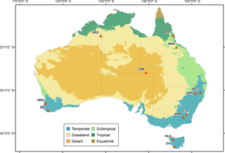
Figure 1 Map of Australian climate zones overlaid by gauging locations plotted as red triangles and labelled with catchment ID. Details of the catchments, including size, are presented in Table 1.

Available ACCESS-S hindcasts are initialised at midnight UTC on days 1 and 25 of each month (additional start dates will become available in the future). A burst ensemble comprising 11 ensemble members is generated. Hindcasts are available for the period 1990–2012 (23 years). A longer hindcast set is not possible because of a lack of suitable initial conditions. The next version of ACCESS-S will be delivered with more sets of initial conditions and longer hindcasts.

2.2 Observed rainfall

Observed rainfall is derived from the Australian Bureau of Meteorology's 5km daily rainfall analysis (AWAP). We make use of AWAP data from 1950 onwards. Catchment rainfall is derived through a process of area-weighted averaging.

An important note on time zones: Australian rainfall is recorded as 24 h totals to 09:00 LT (local time). Consequently, AWAP data are not perfectly synchronised with the ACCESS-S forecasts, which are initialised at midnight UTC. The asynchronism is compounded by time zone differences and daylight savings.

We align the GCM data and observed data as best we can. For east coast locations, an ACCESS-S forecast overlaps with the following day's AWAP rainfall analysis with a discrepancy of 1–2 h. The time discrepancy for west coast locations is approximately 2 h more.

2.3 Catchments

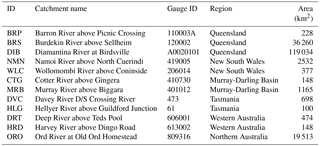
Twelve perennial and ephemeral catchments spread over Australia are selected for application and evaluation. Catchment information including name, gauge ID, regional location and size are shown in Table 1. Catchment locations and climate zones are mapped in Fig. 1. The catchments reside in highly distinct climate zones and vary markedly in size from 100 to 119 034 km². Evaluation across climate zones and for varying catchment sizes helps to comprehensively evaluate the effectiveness of the post-processing methods.

Table 1 Catchment ID, catchment name (river and gauging location), gauge ID, region and catchment size.

3 Methods

3.1 Bayesian joint probability models

Our post-processing method embeds the BJP modelling approach, which was originally designed for forecasting seasonal streamflow totals (Robertson et al., 2013a; Wang and Robertson, 2011; Wang et al., 2009). BJP has since been applied to calibrate hourly rainfall forecasts (Robertson et al., 2013b; Shrestha et al., 2015) and seasonal rainfall forecasts (Hawthorne et al., 2013; Khan et al., 2015; Peng et al., 2014; Schepen and Wang, 2014; Schepen et al., 2014). BJP was most recently adapted for sub-seasonal to seasonal streamflow forecasting (Schepen et al., 2016; Zhao et al., 2016).

BJP formulates a joint probability distribution to characterise the relationship between forecast ensemble means (predictors) and corresponding observations (predictands). The joint distribution is modelled as a bivariate normal distribution after transformation of the marginal distributions. Data transformation is handled using the flexible log −sinh transformation (Wang et al., 2012). The log −sinh transformation transforms y by

$$\begin{array}{}\text{(1)}& {\displaystyle }{\displaystyle }f\left(y\right)={\mathit{\beta }}^{-\mathrm{1}}\ln \left(\sinh \right(\mathit{\alpha }+\mathit{\beta }y),\end{array}$$

where α and β are transformation parameters. A predictor x is transformed to g. Likewise, a predictand y is transformed to h. The relationship between g and h is formulated by a bivariate normal distribution:

$$\begin{array}{}\text{(2)}& {\displaystyle }{\displaystyle }\left[\begin{array}{l}g\\ h\end{array}\right]\sim N(\mathit{\mu },\mathbf{\Sigma }),\end{array}$$

where

$$\begin{array}{}\text{(3)}& {\displaystyle }{\displaystyle }\mathit{\mu }=\left[\begin{array}{l}{\mathit{\mu }}_g\\ {\mathit{\mu }}_h\end{array}\right]\end{array}$$

is the vector of means and

$$\begin{array}{}\text{(4)}& {\displaystyle }\mathbf{\Sigma }=\left[\begin{array}{ll}{\mathit{\sigma }}_g^{\mathrm{2}}& {\mathit{\rho }}_{gh}{\mathit{\sigma }}_h{\mathit{\sigma }}_g\\ {\mathit{\rho }}_{gh}{\mathit{\sigma }}_h{\mathit{\sigma }}_g& {\mathit{\sigma }}_h^{\mathrm{2}}\end{array}\right]\end{array}$$

is the covariance matrix.

In forecasting mode, a BJP model is conditioned on new predictor values. For a particular parameter set, θ, and new transformed predictor value g_new,

$$\begin{array}{}\text{(5)}& {\displaystyle }{\displaystyle }{h}_{\mathrm{new}}\mathrm{|}{g}_{\mathrm{new}},\mathit{\theta }\sim N\left({\mathit{\mu }}_h+{\mathit{\rho }}_{gh}{\displaystyle \frac{{\mathit{\sigma }}_h}{{\mathit{\sigma }}_g}}\left(g_{\mathrm{new}}-{\mathit{\mu }}_g\right),{\mathit{\sigma }}_h^{\mathrm{2}}\left(\mathrm{1}-{\mathit{\rho }}_{gh}^{\mathrm{2}}\right)\right).\end{array}$$

3.2 Daily rainfall post-processing

We note some specifics of the BJP implementation used in this study. To allow the use of the continuous bivariate normal distribution, values of zero rainfall are treated as censored, meaning the true value is assumed to be less than or equal to zero. To simplify the inference of model parameters, data rescaling is used within the modelling process. To prevent undesirable extrapolation effects in forecasting mode, predictor values are limited to twice the maximum predictor value used to fit the model (future research will address this limitation).

Model parameters may be poorly estimated when there are insufficient non-zero data values used in data inference. We find that in very dry catchments, certain days of the year may have forecasts or observations with no non-zero values at all. In such cases, inference is not possible. To overcome this problem, predictor and predictand data sets are created by pooling data for nearby days and for multiple GCM initialisation dates. We choose to pool data within an 11-day sliding window to be consistent with the Bureau of Meteorology's bias correction scheme (see Sect. 3.4); for the first 5 days the window is fixed to the first 11 days. However, the RPP-S method places no restriction on the configuration, and alternative configurations are discussed in Sect. 5. We choose to pool data for ACCESS-S hindcasts initialised on day 1 of the month and day 25 of the month prior. Predictor and predictand data are subsequently paired according to the number of days since forecast initialisation. Consider, for example, post-processing of forecasts initialised on 1 February. Days 5–15 from the 1 February run and days 5–15 from the 25 January run are used to fit a model that is used to post-process forecasts for 10 February.

We note that pooled data are not completely independent, meaning there is potential to underestimate parameter uncertainty using BJP. Nevertheless, we expect the effect to be limited by the weak predictor–predictand relationships and weak persistence in daily rainfall.

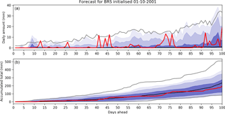
Figure 2 Example RPP-S rainfall forecast for the Burdekin River at Sellheim, initialised on the 1 October 2001 and forecasting 100 days ahead. Forecasts of daily amounts are shown in (a) and forecasts of accumulated totals are shown in (b). Dark blue is the forecast [0.25, 0.75] quantile range; medium blue is the forecast [0.10, 0.90] quantile range; and light blue is the forecast [0.05, 0.95] quantile range. Grey lines are the climatological reference forecast [0.05, 0.95] quantile range. The black line is the climatological reference forecast median. The red line is the observation.

We now describe the model fitting and forecasting steps. After pooling the data, model fitting proceeds as follows:

1. Rescale predictor and predictand data so that each series ranges within [0, 5].

2. Estimate the log −sinh transformation parameters for the predictors using the maximum a posteriori (MAP) estimation.

3. Estimate the log −sinh transformation parameters for the predictands in the same way.

4. Apply the transformations to normalise the predictor and predictand data.

5. Apply the transformations to transform the predictor and predictand censoring thresholds.

6. Sample parameter sets representing the posterior distribution of the bivariate normal distribution parameters using Markov chain Monte Carlo sampling, the transformed data and transformed censoring thresholds.

Forecasting proceeds as follows:

1. Transform the predictor value using the log −sinh transformation for predictors.

2. Sample one h_new for each parameter set.

3. Back-transform the ensemble members using the transformation for predictands.

4. Rescale the ensemble members to the original space (opposite of step 1 in model fitting).

5. Set negative values to zero.

3.3 Forming ensemble time-series forecasts

BJP forecast ensemble members are initially random and are not linked across days. To deal with this problem, we apply the Schaake Shuffle (Clark et al., 2004), which uses historical data to link ensemble members and create sequences with realistic temporal patterns. The Schaake Shuffle works by imposing the rank correlation of observations on the forecast ensembles, using the trajectories of historical observations as a dependence template. Several variations on the Schaake Shuffle exist and choices can be made about how to construct a temporal dependence template. Schefzik (2016), for example, propose selecting historical observations using a similarity criterion. The steps of the Schaake Shuffle as implemented in this study are as follows:

1. Select a large number of years from the past with the same month and day as the forecast initialisation date (excluding the date of the current forecast).

2. Construct a two-dimensional dependence template by incrementing the dates by one day for each day ahead to be forecast.

3. Extract the observed data for each date in the dependence template.

4. For each day, reorder ensemble members according to the rank of the historical data for that day (e.g. if the second year selected has the smallest observed value, place the smallest ensemble member in second position).

5. Repeat steps (2)–(4) for blocks of ensemble members until the full ensemble has been shuffled.

After applying the Schaake Shuffle to all ensemble members across all lead times, the forecasts can be considered ensemble time-series forecasts.

An example RPP-S forecast for the BRS catchment is shown in Fig. 2. The top panel is the forecast of daily amounts and bottom panel is the forecast of accumulated totals. Hereafter, a daily amount is taken to mean a 24 h rainfall total on any given day. An accumulated total is the sum of daily rainfall amounts over a number of days. In this example, the forecast correctly predicts a dry beginning to the forecast period. The quantile ranges of the daily forecasts are reasonably consistent with the observed values. The accumulated forecast is somewhat narrower than the climatology reference forecast at monthly and seasonal timescales and the forecast is predicting a seasonal rainfall total less than the climatological median.

3.4 Verification

We use RPP-S to post-process all available ACCESS-S forecasts initialised on day 1 of each month for 100 days ahead (the sub-seasonal to seasonal forecast period). For water resources management, whilst it is important that daily amounts are realistic, it is vital that the accumulated totals are as reliable and as skilful as possible. Forecasts are verified against both daily amounts and accumulated totals.

RPP-S forecasts are generated using leave-one-year-out cross-validation. RPP-S forecasts are compared with the BOM's QM forecasts (see Sect. 3.5), which are also generated using leave-one-year-out cross-validation.

Bias is recognised as the correspondence between the mean of forecasts and the mean of observations. Bias is visually assessed by plotting the bias for a set of events against the average forecast for the same set of events. We calculate bias as the mean error

$$\begin{array}{}\text{(6)}& {\displaystyle }{\displaystyle }\mathrm{BIAS}:={\displaystyle \frac{\mathrm{1}}{T}}\sum _{t=\mathrm{1}}^T\left({\stackrel{\mathrm{‾}}{y}}_{\mathrm{fcst},t}-y_{\mathrm{obs},t}\right),\end{array}$$

where ${\stackrel{\mathrm{‾}}{y}}_{\mathrm{fcst},t}$ is the forecast ensemble mean for event t and y_obs,t is the corresponding observation. Bias is calculated separately for each catchment, initialisation date and day. The bias is calculated across 23 events. For a given lead time, we also calculate the average absolute bias (AB) across all 12 catchments and 12 initialisation dates. Notwithstanding that the bias is scale dependent, the average absolute bias is used to compare the magnitude of biases for different model forecasts and for different lead times.

Reliability is the statistical consistency of forecasts and observations – a reliable forecasting system will accurately estimate the likelihood of an event. Reliability is checked by analysing the forecast probability integral transforms (PITs) of rainfall observations. The PIT for a forecast-observation pair is defined by π = F(y_obs), where F is the forecast cumulative distribution function (CDF). In the case that y_obs = 0, a pseudo-PIT value is sampled from a uniform distribution with a range [0, π] (Wang and Robertson, 2011). If a forecasting system is reliable, π follows a standard uniform distribution. Reliability can be visually examined by plotting the set of π_t (t = 1, 2, …, T) with the corresponding theoretical quantile of the uniform distribution using the PIT uniform probability plot (or simply PIT plot). A perfectly reliable forecast follows the 1 : 1 line. In this study, we do not plot individual PIT diagrams. Instead, reliability is summarised using the α-index (Renard et al., 2010)

$$\begin{array}{}\text{(7)}& {\displaystyle }{\displaystyle }\mathit{\alpha }=\mathrm{1.0}-{\displaystyle \frac{\mathrm{2}}{n}}\sum _{t=\mathrm{1}}^n\left|{\mathit{\pi }}_t^{*}-{\displaystyle \frac{t}{n+\mathrm{1}}}\right|,\end{array}$$

where ${\mathit{\pi }}_t^{*}$ is the sorted π_t in increasing order. The α-index represents the total deviation of ${\mathit{\pi }}_t^{*}$ from the corresponding uniform quantile (i.e. the tendency to deviate from the 1 : 1 line in PIT diagrams). The α-index ranges from 0 (worst reliability) to 1 (perfect reliability).

Forecast skill is evaluated using the continuous ranked probability score (CRPS; Matheson and Winkler, 1976). The CRPS for a given forecast and observation is defined as:

$$\begin{array}{}\text{(8)}& {\displaystyle }{\displaystyle }\mathrm{CRPS}=\int {\left[F\left(y\right)-H\left(y-y_{\mathrm{obs}}\right)\right]}^{\mathrm{2}}\mathrm{d}y,\end{array}$$

where y is the forecast variable; y_obs is the observed value; F is the forecast CDF; and H is the Heaviside step function, which equals 0 if y < y_obs and equals 1 otherwise. Model forecasts are compared to reference forecasts by calculating skill scores:

$$\begin{array}{}\text{(9)}& {\displaystyle }{\displaystyle }\mathrm{CRPS}\mathrm{skill}\mathrm{score}={\displaystyle \frac{\stackrel{\mathrm{‾}}{{\mathrm{CRPS}}_{\mathrm{ref}}}-\stackrel{\mathrm{‾}}{\mathrm{CRPS}}}{\stackrel{\mathrm{‾}}{{\mathrm{CRPS}}_{\mathrm{ref}}}}}\times \mathrm{100}\left(\mathit{\%}\right),\end{array}$$

where the overbar indicates averaging across a set of events. Reference forecasts for each day are produced using a BJP model fitted to observed data within an 11-day window. The Schaake Shuffle is also applied to instil correct temporal characteristics into the reference forecasts. The CRPS skill score is positively oriented (whereas CRPS is negatively oriented). As a percentage, a maximum score of 100 is indicative of perfectly sharp and accurate forecasts. A score of 0 indicates no overall improvement compared to the reference forecast. A negative score indicates poor quality forecasts in the sense that the naïve reference forecast is more skilful.

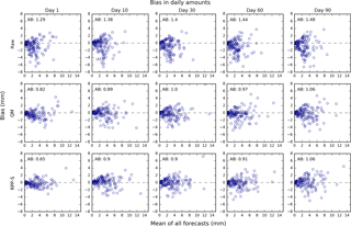
Figure 3 Bias in daily rainfall forecasts for raw, QM and RPP forecasts (rows) and selected days ahead/lead times (columns). The scatterplots are of forecast mean over all events (x axis) versus bias (y axis). There is one blue circle for each catchment and forecast initialisation time. The average absolute bias (AB) is printed in the top left corner.

Figure 4 As for Fig. 3, except for accumulated totals.

3.5 Comparison with forecasts post-processed using quantile mapping

We compare RPP-S forecasts with forecasts that have been post-processed at the ACCESS-S grid scale using quantile mapping (QM). The gridded QM forecasts are supplied by the Bureau of Meteorology and we derive the catchment forecasts through area-weighting. QM matches the statistical distribution of past forecasts to the distribution of observations to reduce errors in the forecast mean and improve forecast spread (Crochemore et al., 2016; Zhao et al., 2017). A post-processed forecast value is obtained by first working out the quantile fraction (cumulative probability) of the new forecast using the CDF of past forecasts, then inverting the quantile fraction using the CDF of observations. The Bureau of Meteorology applied a separate quantile mapping model to each day. The CDF of the past forecasts is formed using 11 ensemble members in an 11-day sliding window and 22 years of data in leave-one-year-out cross-validation. The statistical distribution of the observations is formed using the observations in an 11-day sliding window and 22 years of data. For the first 5 days the window is fixed to the first 11 days. If the raw forecast ensemble member is above the previously known maximum forecast value, then the forecast value is instead linearly rescaled by o_max∕f_max where o_max is the maximum observed value and f_max is the maximum past forecast value.

4 Results

4.1 Bias in forecasts of daily amounts

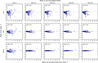
Biases in forecasts of daily amounts are analysed for selected days using Fig. 3. Each circle represents the bias for a catchment and initialisation date. The bias is plotted against the average forecast (averaged over all events). As expected, raw forecasts are more biased than post-processed forecasts. The AB for raw forecasts ranges, for the examples given, from approximately 1.3 to 1.5 mm. The bias for raw forecasts tends to be negative, indicating that ACCESS-S has a propensity to underestimate daily rainfall amounts.

QM and RPP-S are similarly effective at reducing biases in daily amounts and both substantially reduce bias. After post-processing, some residual bias remains for any single day since the bias is corrected using pooled observations. The AB for QM forecasts ranges from roughly 0.8 to 1.1 mm. The AB for RPP-S forecasts ranges from about 0.7 to 1.1 mm. The differences in bias between QM and RPP-S for daily amounts are evidently insignificant. Visual examination of the QM and RPP-S scatter plots shows no wholesale difference in bias between the QM and RPP-S forecasts of daily amounts.

Figure 5 α-index of reliability for forecast daily rainfall amounts (a) and forecast accumulated rainfall totals (b). Results for four types of forecasts are presented: raw, QM, RPP-S before Schaake Shuffle (pre SS) and RPP-S forecasts after the Schaake Shuffle. Higher α-index indicates better reliability. The box plots display the median as a black line. The box spans the interquartile range and the whiskers span the [0.1, 0.9] quantile range.

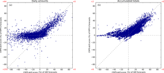
Figure 6 Scatterplots of CRPS skill scores for daily amounts (a) and accumulated totals (b). Results for QM are on the horizontal axis and results for RPP-S are on the vertical axis. Higher CRPS skills scores reflect better forecast performance. Red text preceded by a “+” symbol indicates the number of points plotted outside the axis limits in the quadrant nearest the text.

4.2 Bias in forecasts of accumulated totals

Biases in forecasts of accumulated totals are analysed using Fig. 4 after rescaling to mm day⁻¹. As with the results for daily amounts, the raw forecasts are more biased than post-processed forecasts and the bias tends to be negative. Visual examination of the scatterplots for the raw forecasts reveals, particularly for days 30, 60 and 90, that for some catchments and initialisation times, the raw forecasts are unbiased for sub-seasonal to seasonal rainfall totals. This suggests that the GCM performs well in some regions. Nevertheless, it is evident that post-processing is necessary before using the ACCESS-S forecasts in hydrological forecasting.

In contrast to the results for daily amounts, QM and RPP-S have differing efficacy for reducing biases in accumulated totals, although both still reduce bias substantially. Visual examination of the QM and RPP-S scatter plots shows that the RPP-S points fit more tightly around the zero line than the QM points. The better ability of the RPP-S forecasts to reduce biases is reflected in the AB; for example, for day 90 the AB for QM forecasts is 0.28 mm day⁻¹ and for RPP-S forecasts the AB is 0.13 mm day⁻¹ (cf. the AB for raw forecasts of 0.93 mm day⁻¹).

4.3 Reliability

Reliability is analysed using Fig. 5, which presents box plots of α-index for forecasts of daily rainfall amounts (left panel) and accumulated totals (right panel). The box plots describe the distribution of α-index values for the same cases as we evaluated bias in Sect. 4.2 except that we omit the day 1 result from the accumulated totals analysis. Results are presented for RPP-S before and after the Schaake Shuffle has been applied.

Raw forecasts have the poorest reliability for both daily amounts and accumulated totals. RPP-S has better reliability overall than QM for daily amounts. It is noted that the Schaake Shuffle has no effect on forecast reliability for daily amounts since it is plainly a reordering of already randomised ensemble members.

RPP-S forecasts are more reliable than raw forecasts and QM forecasts for accumulated totals. The RPP-S forecasts become significantly more reliable after applying the Schaake Shuffle and linking the ensemble members so that they have realistic temporal patterns (discussed further in Sect. 5).

4.4 Skill scores – overall performance

Skill scores for QM forecasts are plotted against skill scores for RPP-S forecasts in a scatterplot (Fig. 6). Skill scores for daily amounts are plotted in the left panel; skill scores for accumulated totals are plotted in the right panel. Accumulated totals are for two days or more. RPP-S forecasts and QM forecasts tend to be positively skilful for the same cases, although there is considerable variation in the magnitude of the skill scores. A striking feature of the scatterplots is that when QM forecasts are negatively skilful, the RPP-S forecasts tend to be neutrally skilful, particularly for the accumulated totals. It is evident that skill for daily amounts can be sharply negative. The skill for daily amounts can be difficult to estimate because of the small sample size and the inability to accurately forecast daily amounts beyond about 10 days. In contrast, the skill for accumulated totals is easier to estimate as it benefits from temporal averaging and the accumulation of skill from earlier periods.

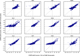
Figure 7 Scatterplots of CRPS skill scores for accumulated totals for each catchment. The scatterplots plot QM skill scores (horizontal axis) against RPP-S skill scores (vertical axis). Each scatterplot combines results for all initialisation dates and all lead times.

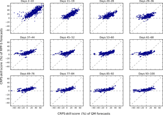
Figure 8 Scatterplots of CRPS skill scores for groups of days (lead times). The scatterplots plot QM skill scores (horizontal axis) against RPP-S skill scores (vertical axis). Each scatterplot combines results for all initialisation dates and all catchments.

Figure 9 Scatterplots of CRPS skill scores for accumulated totals for each initialisation date. The scatterplots plot QM skill scores (horizontal axis) against RPP-S skill scores (vertical axis). Each scatterplot combines results for all catchments and all lead times.

4.5 Skill scores – detailed evaluation

Skill scores are partitioned according to catchment, lead time and initialisation date in Figs. 7–9, respectively. Since forecasts of accumulated totals are more informative for water resources management and forecast skill is generally known to be limited beyond the first week or two, we focus the remainder of the results on accumulated totals.

CRPS skill scores are plotted for each catchment in Fig. 7. Skill scores for RPP-S forecasts are vastly positive except for, most noticeably, some cases in ORO, NMN and HLG. Negative skill can be caused by insufficient information to fit a stable RPP-S model and can also be an artefact of cross-validation in the presence of extreme events. In several catchments, such as WLC and DRT, RPP-S forecasts are seen to significantly outperform QM forecasts by virtue of QM forecasts frequently being significantly negatively skilful and RPP-S forecasts rarely being negatively skilful. In several catchments, including BRP and CTG, both QM and RPP-S skill scores are predominantly positive, demonstrating that simple bias correction techniques can appear sufficient in localised studies.

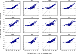
CRPS skill scores are plotted for groups of lead times in Fig. 8. For days 2–10, the RPP-S and QM forecasts are similarly skilful and vastly positively skilful. There are some instances of negative skill, which are likely to be artefacts of cross-validation. For days 11–19 and 20–28, the positive relationship between QM and RPP-S forecasts gradually weakens. From day 29 onwards, the QM forecasts become negatively skilful in many instances whereas the RPP-S skill scores tend to level out around zero and are rarely negative to the same degree. For very long lead times, QM skill scores can be higher than RPP-S skill scores, although overall the skill scores for accumulated seasonal totals are quite low (< 30 %). Both these factors signal further improvement in the RPP-S forecasts is possible.

CRPS skill scores are plotted for each initialisation date in Fig. 9. Forecasts initialised from 1 September to 1 November have the highest proportion of cases where both QM and RPP-S forecasts are positively skilful, suggesting that ACCESS-S produces its best sub-seasonal to seasonal forecasts during the Austral spring and summer.

5 Discussion

We demonstrate that RPP-S is able to improve daily GCM rainfall forecasts by: reducing bias (Figs. 3–4); improving reliability (Fig. 5); and ensuring that forecasts are typically at least as skilful as a climatological reference forecast (Figs. 6–9). RPP-S forecasts are comprehensively compared with QM forecasts. RPP-S forecasts outperform QM forecasts, primarily because QM does not take into account the correlation between forecasts and observations nor corrects for autocorrelation problems. Since RPP-S is built upon the BJP modelling approach, it explicitly models the correlation between the forecasts and observations, and thus takes into account model skill in the calibration. Our results add to the findings of Zhao et al. (2017) who studied the post-processing of monthly rainfall forecasts from POAMA (Australia's GCM preceding ACCESS-S). While Zhao et al. (2017) demonstrated that QM is very effective for bias correction, they did not consider accumulated totals. In our study, we find that the RPP-S forecasts are less biased and more reliable than QM forecasts for accumulated totals.

Figure 5 illustrates the importance of the Schaake Shuffle for producing reliable forecasts using RPP-S. If the forecasts are not shuffled, then the forecasts of accumulated totals will tend to be too narrow in terms of ensemble spread, making the forecasts over-confident and less reliable. Related to this, RPP-S forecasts are more reliable for daily amounts than QM forecasts, yet QM and RPP-S forecasts do not exhibit any obvious differences in the magnitude of biases (Fig. 3) – evidence that the RPP-S forecasts have a more appropriate ensemble spread, since the α-index integrates information about forecast bias and ensemble spread.

We applied a consistent methodology to perennial and ephemeral catchments and established BJP models separately for each day, catchment and initialisation date. Alternative configurations are also possible, for example, we trialled establishing only six models by pooling data within week 1, week 2, weeks 3–4, and subsequent 4 week periods (not shown). The data in week 1 were used to fit model BJP1, the data in week 2 were used to fit model BJP2, and so on. Fewer days were pooled close to the initialisation date in an attempt to extract skill from the initial conditions and more days were pooled for longer lead times to better approximate the climatological distribution. We found significant efficiency gains with little loss in performance, except for dry catchments, where a small increase in the frequency of negative skill scores occurred. Therefore, performance and efficiency need to be considered when establishing RPP-S models in new catchments.

The RPP-S method is sophisticated in that it is a full calibration approach, however, there are opportunities to improve the methodology. By pooling the data for many days in model parameter inference for example, it is assumed that rainfall from one day to the next is independent, which is an oversimplification. New inference methods that treat the rainfall data as conditionally independent therefore ought to be investigated. Future studies will seek to address the matters of independence and overlapping data in more sophisticated ways.

We make use of ACCESS-S runs initialised on day 1 of the month and day 25 of the previous month. These initialisation dates are only 4–7 days apart and therefore the climatology of daily rainfall is unlikely to change significantly over this period of time. It is technically possible to establish an RPP-S model using initialisation dates spanning several months. If temporally distant initialisation dates are included in model parameter inference, new strategies may be needed to ensure that the effects of seasonality are minimised. One possible approach is to standardise forecasts and observations prior to fitting the BJP model. In this way, the model transformation and climatological parameters will be allowed to vary by day of year. Such strategies for building more robust RPP-S models and coincidentally minimising the effect of seasonality will be investigated in follow up work.

RPP-S and QM CRPS scores are calculated using ensembles of different sizes and we consider the effect of ensemble size on our results. When a forecasting system is perfectly reliable, a larger ensemble should yield a better CRPS score (Ferro et al., 2008). However, CRPS has a weakness in that it discourages forecasting extremes (Fricker et al., 2013); indeed it is our experience that ensembles that are unbiased but too narrow (like the QM forecasts) can score overly well in terms of CRPS. Our position is that because the RPP-S and QM forecasts are not similarly reliable, we are unable to make meaningful adjustments to CRPS scores to allow for the effect of ensemble size. In any case, we understand that QM forecasts can be significantly negatively skilful and unreliable, and small adjustments to the CRPS of QM forecasts will not affect those conclusions.

RPP-S is designed to post-process forecasts of daily amounts. An alternative strategy is to post-process accumulated totals and subsequently disaggregate to daily amounts. BJP models may be applied to post-process monthly and seasonal totals, which are then disaggregated to daily timescales. Future work will investigate the relative merits of direct daily post-processing versus a seasonal calibration and disaggregation approach. This follow-up work is of particular interest as our study has shown daily post-processing skill is limited beyond 10-15 days. It is not clear how much of the seasonal forecasting skill is attributable to skill in the initial period and how much of the skill is attributable to seasonal climate signals in the GCM.

While our study has focused on rainfall, other variables are important in hydrology. Temperature forecasts, for example, are required in areas of snowmelt. Therefore, future research will investigate the extension of the RPP-S ideas to include other meteorological variables.

An alternative to statistical post-processing of GCM outputs is to run a regional climate model (RCM) to provide much more localised information than a global GCM. A review study by Xue et al. (2014) found that RCMs have limited downscaling ability for sub-seasonal to seasonal forecasts. In that regard, RCM outputs may also be statistically post-processed, which may lead to better forecasts in some regions. RCMs are suited to specialised studies and less suited to post-processing operational GCM forecasts in support of national scale hydrological forecasting services.

6 Conclusion

We have developed a novel method for post-processing daily rainfall amounts from seasonal forecasting GCMs. RPP-S is a full calibration approach that makes use of the BJP modelling approach to account for predictor–predictand skill relationships in post-processing. Reliable forecasts of sub-seasonal and seasonal accumulated totals are produced by linking ensemble members together using the Schaake Shuffle.

We applied RPP-S to 12 catchments across Australia in diverse climate zones. The method is robust in terms of being capable of post-processing forecasts in all cases, even in very dry catchments.

Compared to raw forecasts and QM post-processing (which does not account for predictor–predictand skill relationships), RPP-S performs significantly better in terms of correcting bias, reliability and skill. The only exception to this conclusion is that QM and RPP-S are similarly effective for correcting biases in daily amounts. RPP-S is particularly effective at delivering reliable, skilful, monthly and seasonal rainfall forecasts. Thus RPP-S forecasts are highly suitable for feeding into hydrological models for seasonal streamflow forecasting and other water resources management applications. Pooling multiple GCM runs and data for adjacent days in model parameter inference is a practical measure that can enable statistical post-processing across a range of perennial and ephemeral streams. There are many avenues of research that could significantly improve the robustness and performance of RPP-S forecasts. In the future, more effort could be devoted to applying RPP-S more widely and relating forecast performance to catchment characteristics, therefore yielding a better understanding of forecast bias, reliability and skill.