
the Creative Commons Attribution 4.0 License.
the Creative Commons Attribution 4.0 License.
 | 27 Jul 2026
Hybrid models generalize better to warmer climate conditions than process-based and purely data-driven models
Jan P. Bohl
Corinna Frank
Paul C. Astagneau
Jonas Peters
Manuela I. Brunner
Deep learning-based rainfall-runoff models, in particular long short-term memory networks (LSTM), have been shown to outperform traditional hydrological models at various tasks, both when used as purely data-driven models and when combined with process-based models in a hybrid setting. These tasks include predictions in ungauged basins (PUB) and regions (PUR), tasks which have traditionally been challenging for conceptual hydrological models. While the spatial generalizability of deep learning-based models has received a lot of attention, it is less clear how they generalize to unseen and warmer climate conditions, i.e. how suitable these models are for hydrological climate impact studies. To address this research gap, we assess the ability of three types of models including (1) fully data-driven (LSTMs), (2) conceptual (Hydrologiska Byråns Vattenbalansavdelning; HBV), and (3) hybrid (differentiable hydrologic models) to simulate streamflow under conditions warmer than those used to train the models by running a differential split sample test. That is, we trained the models using data from the historical period 1960–1990 and evaluated them on data of this period as well as of the warmer period 2000–2023. We find that the LSTM is the most accurate model overall (median NSE: 0.74–0.79), followed by the hybrid (median NSE: 0.68–0.71) and HBV model (median NSE: 0.53–0.56). However, the LSTM shows a stronger change in performance between the warm and cold period (NSE: −0.05 to −0.04) compared to the hybrid (NSE: −0.03–0) and HBV model (NSE: −0.03 to −0.02). When comparing observed with simulated streamflow signals, we find a higher sensitivity of the LSTM to changes in meteorological forcings (mainly temperature change) for mean flows (MQ: −8.5 % to −12.6 %) and high flows (Q99: −7.0 % to −13.4 %) than in observations (MQ: −4.6 % to −9.4 %, Q99: −3.6 % to −9.7 %). In contrast, the hybrid and HBV model show good agreement with observed change signals. These findings indicate that the LSTM, while being the most accurate overall, has a lower generalizability to warmer conditions than the other models. However, we also find that the models' capability to generalize can differ between catchment type. While all models generalize better in rainfall-dominated catchments, they all show larger but similar reductions in performance in snow-dominated catchments. This suggests that all models struggle to generalize to warmer conditions in snow-dominated catchments implying that better process-representation in the models might be needed to accurately capture the dynamics of snow-melt and -accumulation processes, which are highly sensitive to changes in temperature. We conclude that hybrid models effectively combine the strengths of LSTMs in having a high accuracy when predicting in ungauged basins, with the good generalizability under changes in climate from the conceptual hydrological models. This makes hybrid models a suitable choice for hydrological climate change impact assessments, particularly in ungauged basins.
- Article
(4211 KB) - Full-text XML
- BibTeX
- EndNote


Many hydrological applications, such as water resources management (Keller et al., 2023), hydraulic engineering (Páez Mendieta et al., 2024), and flood and drought forecasting (Xing et al., 2020; Brunner et al., 2021b), build on long-term future streamflow predictions because climate change is expected to have significant effects on the water cycle (Gudmundsson et al., 2021). Hydrological climate impact assessments that quantify these effects heavily rely on rainfall-runoff models, which allow modellers to translate future climate scenarios into hydrological predictions (Van Der Wiel et al., 2019; Sauquet et al., 2021; Lemaitre-Basset et al., 2021; Muelchi et al., 2022; Willkofer et al., 2024).
Historically, process-based conceptual hydrological models have been used to perform such climate impact assessments (Hakala et al., 2019). They approximate the hydrology of catchments by representing water storage components such as snowpack, soil moisture, and groundwater, as well as the fluxes between them including percolation, snowmelt and evapotranspiration (Lindström et al., 1997; Clark et al., 2017). Most of these models have parameters that need to be calibrated against observations to obtain accurate streamflow predictions (Wagener et al., 2003; Beven, 2012; Andréassian et al., 2014). These parameters are usually calibrated on individual catchments, often using streamflow time series recorded at their outlet (Beven, 2012). Because of their reliance on observations, calibrated hydrological models struggle to generalize in time and space (Vaze et al., 2010; Hrachowitz et al., 2013; Fowler et al., 2018a), meaning that there are strong reductions in accuracy when applying them to time periods and regions unseen during calibration. This limits their reliability for climate change impact assessments that look far into the future and applications in ungauged basins, i.e. basins where streamflow observations are missing (Hrachowitz et al., 2013).
Deep learning streamflow models, in particular long short-term memory networks (LSTMs; Hochreiter and Schmidhuber, 1997), have in the past few years been proposed as a data-driven alternative to conceptual models. LSTMs (Hochreiter and Schmidhuber, 1997) are a type of Recurrent Neural Network (Rumelhart et al., 1987), which address the problem of vanishing and exploding gradients and are thus able to learn long-term dependencies. This is crucial when simulating streamflow because of the substantial memory of the hydrological system (Berghuijs et al., 2025). They have been shown to outperform conceptual models for rainfall-runoff modelling in gauged basins, i.e. basins where streamflow observations are available for model calibration (Kratzert et al., 2018, 2019b; Mai et al., 2022). These models have no prior process knowledge and are optimized to learn the relationship between streamflow data and meteorological forcing data such as precipitation and temperature. In contrast to conceptual models, which are parametrized individually for each catchment, LSTMs perform best when learning from large regional datasets (Kratzert et al., 2019b, 2024). These models also excel at tasks which have historically been challenging for conceptual rainfall-runoff models, notably prediction in ungauged basins (Kratzert et al., 2019a) or regions (Feng et al., 2021). However, it is often hypothesized that these purely data-driven models might struggle with extrapolation to, in particular warmer, climate conditions unseen during training (Wi and Steinschneider, 2022, 2024; Reichert et al., 2024). This assumption is supported by general machine learning research, which has shown that data-driven models trained with standard objective functions tend to perform poorly under distribution shifts in the input variables (Koh et al., 2021; Liu et al., 2021; Wang et al., 2022).
In an attempt to overcome this limitation while profiting from the strengths of both conceptual (i.e. interpretability) and data-driven models (i.e. generalizability to ungauged basins), hybrid hydrological models have recently gained interest as an additional modelling alternative (Frame et al., 2021; Höge et al., 2022; Kraft et al., 2022; Slater et al., 2023). Hybrid modelling combines deep learning with traditional hydrological modelling – a concept which has been successful in various research fields (Karpatne et al., 2017). A hybrid approach can be as simple as using an LSTM to post-process the outputs or internal states of a conceptual model (Frame et al., 2021; Liu et al., 2024). Other hybrid approaches replace parts of the structure of a conceptual or physically-based model with data-driven models (Höge et al., 2022; Kraft et al., 2022) or use deep parameter learning to estimate the parameters of conceptual models from data (Tsai et al., 2021; Feng et al., 2022a; Shen et al., 2023). For example, LSTMs can be used to dynamically predict the parameters of an ensemble of HBV models – an approach which has been shown to have similar accuracy as a stand-alone LSTM model for rainfall-runoff modelling (Feng et al., 2022a). Hybrid models have also been shown to rival the performance of stand-alone LSTMs when predicting streamflow in ungauged basins (Feng et al., 2023). For more challenging spatial extrapolation tasks, such as prediction in ungauged regions that have been left out from the training dataset, hybrid models even outperform LSTMs (Feng et al., 2023, 2024). In addition, some hybrid models have shown promising results in climate sensitivity analyses that tested how realistically hybrid models represent streamflow sensitivities to changes in meteorological forcing (Wi and Steinschneider, 2022, 2024). These sensitivity analyses suggest that hybrid models may also be a promising alternative for climate change impact assessments. However, it still needs to be quantitatively assessed how well they generalize to warmer climate conditions as compared to conceptual and purely data-driven models such as LSTMs. We use the term generalizability for the change in accuracy between a reference period with climate similar to the calibration period and a testing period with different climatic conditions. A model is thus considered to generalize well if it experiences little change in accuracy between different climatic conditions.
Conceptual hydrological models are known to suffer from reductions in accuracy when evaluated on periods whose climate differs from the one in the calibration period (Vaze et al., 2010; Coron et al., 2012; Fowler et al., 2016; Dakhlaoui et al., 2017; Guo et al., 2020; Ji et al., 2023). In contrast, there is still little research on the behaviour of LSTMs and hybrid models under changing climate conditions. Bai et al. (2021) have found that LSTMs show larger reductions in accuracy when evaluated under climate conditions drier/wetter than those of the calibration period compared to conceptual hydrological models. Metamorphic testing (Reichert et al., 2024) and climate sensitivity analyses have been used to compare the response of LSTMs to the one of conceptual hydrological models (Wi and Steinschneider, 2022, 2024; Reichert et al., 2024; Martel et al., 2025). These studies have shown that LSTMs react differently to changes in climate than conceptual hydrological models and that their response is in some cases opposite to what would be expected based on process understanding. Notably, the sign of the streamflow response to changes in climate can depend on the hyper-parameters and training set used for modelling (Reichert et al., 2024), which is problematic when applying LSTMs for the purpose of hydrological climate impact assessments. To strengthen the generalizability of LSTMs to unseen climate conditions, Wi and Steinschneider (2022, 2024) have proposed to add physical constraints to the data-driven models by enforcing mass-conservation. Furthermore, they have proposed to train regional/national models on a larger set of catchments outside of the target domain to cover a broader range of catchment and climate characteristics. While Reichert et al. (2024) did not find improvements in the physical realism of LSTM simulations when training the model on additional catchments, Wi and Steinschneider (2022, 2024) have shown that such geographically extended models produce more realistic simulations than regional LSTMs only trained with the catchments of the study area. This finding suggests that these models may similarly be more suitable for extrapolating to unseen conditions different from those seen during training.
Such extrapolation includes predicting extreme events. This modelling task is crucial within the framework of climate impact assessments because these events have been shown to become more frequent and intense with observed (Dai, 2013; Berghuijs et al., 2019; Bertola et al., 2020), and future projected climate change (Madsen et al., 2014; Brunner et al., 2021c; Willkofer et al., 2024; Gebrechorkos et al., 2025). Model evaluation studies have shown that both conceptual and data-driven models are challenged by the task of simulating extreme events such as floods (Mizukami et al., 2019; Brunner et al., 2021a; Baste et al., 2025; Santos et al., 2025) and droughts (Fowler et al., 2016; Bruno et al., 2024). Synthetic experiments have shown that LSTMs tend to outperform conceptual and physically-based models (Frame et al., 2022) in simulating floods with magnitudes larger than those included in the training data. However, compared to hybrid models, LSTMs underestimate the most severe floods (Acuña Espinoza et al., 2025; Baste et al., 2025). For low flows, Kratzert et al. (2019b) have shown that many conceptual and physically-based hydrological models are more accurate than pure LSTMs in gauged catchments. In contrast, LSTMs have been found to outperform hybrid and conceptual hydrological models in simulating low flows in ungauged basins (Feng et al., 2023). Therefore, the simulation of extreme events under changing climate conditions with data-driven models is gaining attention. Feng et al. (2023) have shown that hybrid models simulate high flows more accurately than LSTMs, while LSTMs perform equally well as hybrid models for low flows. The question is how well these results obtained for current climate conditions translate to extreme events simulated for unseen climate conditions.
Changes in extreme events can be particularly pronounced in mountain regions, where snow and glaciers play an important role in the water cycle (Schwarb, 2000; Beniston, 2006; Mountain Research Initiative EDW Working Group, 2015). Snowmelt and accumulation are highly sensitive to changes in air temperature (Frei et al., 2018). As a result, warming affects the seasonality and magnitude of streamflow regimes (Barnett et al., 2005; Freudiger et al., 2020; Uzun et al., 2021), extreme events (Blöschl et al., 2017; Brunner et al., 2019), and their generation processes (Brunner et al., 2023) in Alpine areas. Models thus need to accurately parametrize snow-related processes in order to generalize well to unseen climate conditions. To represent snow, conceptual models typically use a simple degree-day factor approach, which determines the degree of melting during a single day by considering air temperature (DeWalle, 2008). This simple approach generally leads to accurate streamflow simulations in snow-dominated catchments (Braun and Renner, 1992), while leaving some room for further improvement (Girons Lopez et al., 2020). In contrast to conceptual models, LSTMs do not explicitly represent snow-related processes and little is known about the behaviour of LSTMs and hybrid models in snow-dominated catchments. The few existing studies on the topic suggest that LSTMs generally perform well compared to conceptual hydrological models in regions with snow-dominated catchments (Arsenault et al., 2023; Kraft et al., 2025) and have a slight advantage over hybrid models in cold and polar climates (Feng et al., 2024).
Some of the model evaluation studies mentioned above have studied some specific aspects of model generalizability between different model types, i.e. conceptual, data-driven, and hybrid. However, it is yet unclear which type of hydrological model is most suited for long-term predictions of streamflow and extreme events under climate change in mountain regions and how model accuracy and generalizability are linked. Here, we shed new light on the accuracy-generalizability trade-off of deep learning hydrological models in mountain regions by addressing the following research questions:
-
How do data-driven and hybrid models generalize to warmer climatic conditions compared to conceptual models?
-
How does the generalizability of conceptual, data-driven, and hybrid models differ for extreme events vs. all types of streamflow conditions?
-
How does the generalizability of these models differ for snow-dominated vs. rainfall-dominated catchments?
To address these research questions, we perform a differential split sample test (DSST; Klemeš, 1986; Seibert, 2003; Coron et al., 2012) on a dataset of 918 catchments in Central Europe for three different types of models: (a) a conceptual model (HBV, Bergström, 1976; Lindström et al., 1997; Seibert and Vis, 2012), (b) a data-driven model (LSTM, Kratzert et al., 2019b, 2022), and (c) a hybrid model (differentiable hydrologic model, Feng et al., 2022a, 2023). We train the models on a “cold” reference period (1960–1990) and evaluate them on a testing period (2000–2023) whose climate is on average warmer than the one of the training period. To be suitable for climate change simulations, the models need to (a) be accurate and (b) generalize well to unseen warmer climate conditions. To evaluate the models with respect to these two targets, we on the one hand use standard accuracy metrics, and on the other hand quantify the change in those metrics between the training and extrapolation periods. In addition to testing for general model accuracy, we also consider metrics which test the models' ability to predict extreme events (high- and low-flows) and investigate whether the models generalize equally well in snow- vs. rainfall-dominated catchments.
Our results highlight that the model with the highest accuracy in a spatial regionalization context is not necessarily the one with the best generalizability to warmer climate conditions than those seen during model training. Among the three model types considered, the LSTM shows the highest accuracy – both for mean and extreme flows –, while the hybrid model generalizes best under distribution shifts in meteorological forcing. For snow-dominated catchments, all models suffer from similar reductions in accuracy when simulating streamflow under unseen climate conditions and the LSTM is the most accurate model for all periods.
2.1 Data
For our model-intercomparison study, we assembled streamflow observations, catchment-averaged meteorological data, and static catchment attributes for a large sample of 918 catchments in Central Europe (Fig. 1). The study domain covers the European Alps and the lowland regions around them, specifically the three major river basins originating in the Central Alps: the Danube, Rhine, and Rhône. It includes catchments in southern Germany (Bavaria and Baden-Württemberg), Austria, Switzerland, and eastern France (Rhône and Rhine basins). Streamflow data for these regions were collected from national agencies in Austria (Austrian Ministry of Sustainability and Tourism), Switzerland (Federal Office of the Environment, FOEN), and France (Banque HYDRO). Regional offices provided the streamflow data for the German states of Bavaria (Bavarian State Office for the Environment) and Baden-Württemberg (State Institute for the Environment Baden-Württemberg). We had to exclude Italy from our analysis because none of the streamflow time series collected for northern Italy (Piemonte, Lombardia, Valle d'Aosta) had data records for the cold period that were sufficiently long for model training.
We selected near-natural catchments only, as we wanted to assess how well the different model types represent the link between climatic variables and streamflow. To identify these catchments, we used information on reservoir locations and characteristics collected from national and regional agencies (Austria: Simmler, 1962; Partl, R., 1977, Switzerland: Swiss Federal Office for Energy, Germany: Speckhann et al., 2021, France: Comité Français des Barrages et Réservoirs, 2022, see Götte et al., 2025, for details). We limited ourselves to catchments with a degree of regulation (reservoir volume relative to annual streamflow volume) below 10 %. Following Klotz et al. (2025), we also excluded catchments which are smaller than 50 km2 or have anomalous streamflow signatures (mean specific discharge smaller than 0.1 mm d−1 or larger than 10 mm d−1). We also excluded catchments with insufficient data records (fewer than 10 years of streamflow data in the 1960–1990 period), too many missing values (more than 10 %) or with problems in the data, such as multiple observations for a single day or too many repetitive values (more than 50 %).
We extracted a set of catchment-averaged daily meteorological variables from the E-OBS v29.0 gridded dataset at a resolution of 0.1° (Copernicus Climate Change Service, 2020), namely precipitation, minimum, mean, and maximum daily temperature, potential evapotranspiration, and incoming shortwave radiation. The aggregation was performed using area-weighted means within catchment boundaries with the Python Xagg library (Schwarzwald and Geil, 2024). Additionally, we compiled SWE data for Switzerland and Austria as reference datasets for evaluating the snowpack simulated by the conceptual and hybrid models. For Austria, we used the SNOWGRID-CL (Olefs et al., 2020; GeoSphere Austria, 2022) dataset, which represents SWE over Austria on a 1 km × 1 km grid and covers the time period from January 1961 until 24 April 2024. It was created using a 2-layer energy balance model with data assimilation of snow height measurements. For Switzerland, we used the OSHD-CLQM (Michel et al., 2024; Marty et al., 2025) dataset which is based on a simple temperature index model with quantile mapping and is available on a 1 km × 1 km grid from September 1961 until September 2021.
From the observed streamflow, the catchment-averaged meteorological variables, and other data sources, we derived a set of hydroclimatic catchment characteristics (Table A1). Catchment characteristics describing the land-use, geology, topography, soil composition and glacier characteristics were derived from the HydroATLAS dataset (Linke et al., 2019; Lehner et al., 2022) using the procedures proposed in the CARAVAN dataset (Kratzert et al., 2023).
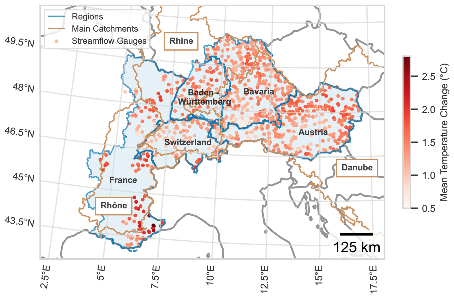
Figure 1The 918 catchments used in this study, spread across different countries and river basins. The colors of the corresponding gauges indicate the change in mean temperature between the cold (training; 1960–1990) and warm (testing; 2000–2023) period.
2.2 Models
In this study, we considered three types of models and compared them with respect to four key metrics for hydrological climate impact assessments (see Fig. 2a for an overview of the workflow). We compared (1) their absolute accuracy, (2) their generalizability to a warmer climate (i.e. change in accuracy between the cold training period and the warmer testing period) and (3) their ability to simulate extreme events in ungauged basins, and (4) their ability to simulate observed streamflow signals. The three types of models are: (1) a conceptual process-based model, specifically the HBV model, (2) a data-driven model, specifically an LSTM, and (3) a hybrid model, specifically the differentiable hydrologic δ-HBV model. To compare accuracy and generalizability metrics between two hydrological models, we used the sign test (Mendenhall et al., 1990), which determines the statistical significance of differences between models across catchments. For metrics where larger scores correspond to better accuracy (such as the NSE and KGE), we used the one-sided sign test, for all other metrics (such as biases), we used the two-sided sign test.
2.2.1 HBV
The HBV model is a conceptual model widely used in hydrological research (Bergström, 1976; Seibert and Bergström, 2022). It represents hydrological processes such as snow storage, soil moisture and groundwater as buckets connected by fluxes such as snowmelt, surface runoff, groundwater flow and evapotranspiration, while respecting mass conservation. The empirical equations relating the different processes are based on physics and observations. The HBV implementation used in our experiments is based on HBV-light (Seibert and Vis, 2012), with slight modifications proposed by Feng et al. (2022a). It has 14 parameters and the meteorological inputs passed to the model are listed in Table A2. In our analysis we distinguish between two different HBV setups: (a) HBV (in-sample) which was calibrated for each catchment separately, and (b) HBV (regional) which infers model parameters from donor catchments and represents a model setup for ungauged basins. To obtain predictions for the HBV regional model, we employed the regionalization scheme outlined in Beck et al. (2016) with slight modifications. For a given target catchment, this scheme determines 10 donor catchments among the set of calibrated catchments (HBV (in-sample) excluding the catchment being modelled) through a similarity measure based on seven catchment attributes describing the catchments' climate, topography and soil type (Table B2). The similarity is computed as
where i,j represents a basin index, p indexes the attributes, represents the vector of attributes for basin i, and IQRp represents the interquartile range for attribute p. We used the parameter sets of the 10 most similar catchments to simulate streamflow using the meteorological forcings of the target catchment. The resulting streamflow time series are then averaged and used as the streamflow prediction for the target catchment. This regionalization approach is simple to implement and has been shown to perform well (Beck et al., 2016), but its accuracy decreases with decreasing density of streamflow gauges in the regionalization domain (Oudin et al., 2008). If not explicitly mentioned otherwise, the standard HBV setup used for the model comparison is the regional HBV and is simply referred to as HBV.
2.2.2 LSTM
The LSTM is a purely data-driven model, which learns the relationship between meteorological forcings and streamflow observations through the optimization of an objective function (Kratzert et al., 2018, 2019b). It thus includes no prior process knowledge and has no enforced physical constraints. We implemented a regional LSTM based on the model proposed in Kratzert et al. (2019b). A single model is trained to predict streamflow from catchment characteristics and meteorological forcings for a diverse set of catchments. Compared to the setup by Kratzert et al. (2019b), we replaced the linear activation function used there by a Rectified Linear Unit (ReLU)
Together with the normalization of the training data described in Sect. 2.3, this ensures that the model output is non-negative. The static catchment attributes and meteorological variables used as input variables are listed in Tables A1 and A2.
2.2.3 Hybrid model
We considered the hybrid model δ-HBV that combines the conceptual HBV model (15 parameters) with an LSTM for parameter estimation. This approach has the advantage of a physically consistent treatment of meteorological variables (such as conservation of mass) and gives access to untrained variables such as snowpack, soil moisture, and evapotranspiration. We restricted ourselves to the most flexible structure proposed in the original studies by Feng et al. (2022a, 2023), denoted there as δ16(β,γ). This structure consists of 16 parallel HBV models that represent heterogeneity within catchments and have a dynamic rainfall-runoff coefficient (β) and evapotranspiration factor (γ) to account for the seasonality in the underlying processes. These two parameters were dynamically predicted for each day of the simulation period by the LSTM. The remaining 13 parameters of the HBV model and the two parameters of the routing model were also predicted by the LSTM but were kept constant during each evaluation period. The LSTM component of the hybrid model received the same static catchment attributes and meteorological inputs as the stand-alone LSTM (Table A2). The parameters predicted by the LSTM were then used to process the meteorological variables also passed to the stand-alone HBV model to predict streamflow (Table A2).
2.3 Training & Calibration
All models were calibrated with data from the 1960–1990 period, which we used as a reference period representing cold climate conditions. To ensure consistency between the three models, we used the Nash-Sutcliffe efficiency (NSE; Nash and Sutcliffe, 1970) to calibrate all models. We chose the NSE because it is the most commonly used objective function when training LSTMs for streamflow modelling. Specifically, we used the classical NSE on a catchment level for the HBV model and the smooth-joint NSE proposed by Kratzert et al. (2019b) for the LSTM and hybrid models. The HBV model was calibrated for each catchment using 1000 iterations of the DDS Algorithm (Tolson and Shoemaker, 2007). For predictions in ungauged basins, we used the regionalization scheme described in Sect. 2.2. The two deep learning models were trained using the Adam algorithm (Kingma and Ba, 2017). It is common practice to standardize the input and output data of deep learning models to improve the stability of the optimization procedure (LeCun et al., 2012). We therefore standardized the static catchment attributes and input time series passed to the LSTMs to have zero mean and unit variance, while the inputs to the conceptual model were left unchanged. Following Kraft et al. (2025), the specific discharge time series were divided by the 95th streamflow quantile across all catchments when training the stand-alone LSTM. Together with the ReLU activation function, this ensures positive predictions.
To determine the best hyper-parameters for the optimization of the LSTM and hybrid models, we performed a small grid search using a validation set consisting of 128 catchments. The validation set consisted of catchments which had more than 5 years of streamflow data in the 1960–1990 period but did not meet our requirement of having at least 10 years of data in that period. These catchments were not used for training or any further analyses. The set of hyper-parameters determined with this approach can be found in Table B1. With these hyper-parameters, we trained an ensemble of models using spatial cross-validation (Kratzert et al., 2019a) by randomly splitting the catchments into 5 equally sized folds. For each target fold, the remaining 4 folds were used to train 5 models with different random initializations. Thus, we trained 25 LSTMs and 25 hybrid models in total. We then averaged the predictions of the 5 models to obtain a single ensemble prediction for every fold. Every catchment was thus held out exactly once from training.
2.4 Evaluation
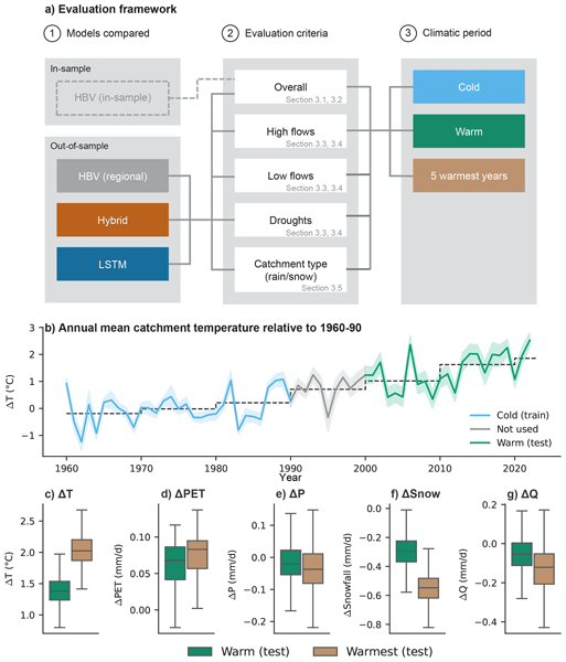
To evaluate the generalizability of the different models across different climatic conditions, we quantified their performance for a variety of metrics under a cold, warm and warmest period (Fig. 2a). This allowed us to assess the change in accuracy when predicting streamflow in a warmer climate, for which the models were not trained. We chose these periods based on the decadal mean temperature (Fig. 2b). During the cold period (1960–1990), the mean temperature was relatively constant and lower than in later decades. Therefore, it was chosen as the training period. For the warm period (testing), we used only decades for which the decadal mean is +1 °C above that of the period 1960–1990, resulting in the testing period 2000–2023, to ensure a substantial warming effect between the training and testing periods. To assess the effect of even stronger warming on model accuracy and generalizability, we also considered a second evaluation period, namely the “warmest” period, consisting of the 5 warmest years during the warm period for each catchment. These three scenarios (cold, warm and warmest) are distinct in terms of their climatic conditions and streamflow responses (Fig. 2c–g). In terms of the median across catchments, the mean temperature increased by 1.4 °C between the cold and the warm period and by 2.0 °C between the cold and the catchment-specific warmest periods. The largest differences between the warm and warmest periods are observed in the temperature and snowfall variables, while potential evaporation and precipitation only show small changes.
In addition to the out-of-time evaluation, given by the three different periods, we also evaluate the models for the prediction of streamflow in ungauged basins (i.e. out-of-sample) in a total of 918 catchments. Specifically, we evaluated the models on the subset (fold) of catchments which was not used to calibrate or train the models. The combination of the out-of-time and out-of-sample evaluation is necessary to limit the influence of overfitting on the training data. This enables us to compare the model simulations across climatic periods without relying on training data. The HBV model was also evaluated in gauged catchments to evaluate the effectiveness of the regionalization scheme and provide a reference model typically used for climate change impact analyses. We refer to this model as the in-sample HBV as opposed to the regional HBV. To evaluate the overall model accuracy, we used the following evaluation metrics (see also Table C1): the NSE and the Kling-Gupta efficiency (KGE; Gupta et al., 2009) as well as its components, namely bias (βKGE), variance (αKGE), and correlation (r) (Gupta et al., 2009). Please note that we evaluated the hybrid model separately for the 1960–1990 and 2000–2023 periods to allow the model to adapt the static parameters to the climate conditions of the different periods, resulting in two distinct parameter sets. For the 5 warmest years, we did not conduct a separate evaluation and the static parameters were thus the same as those of the warm period.
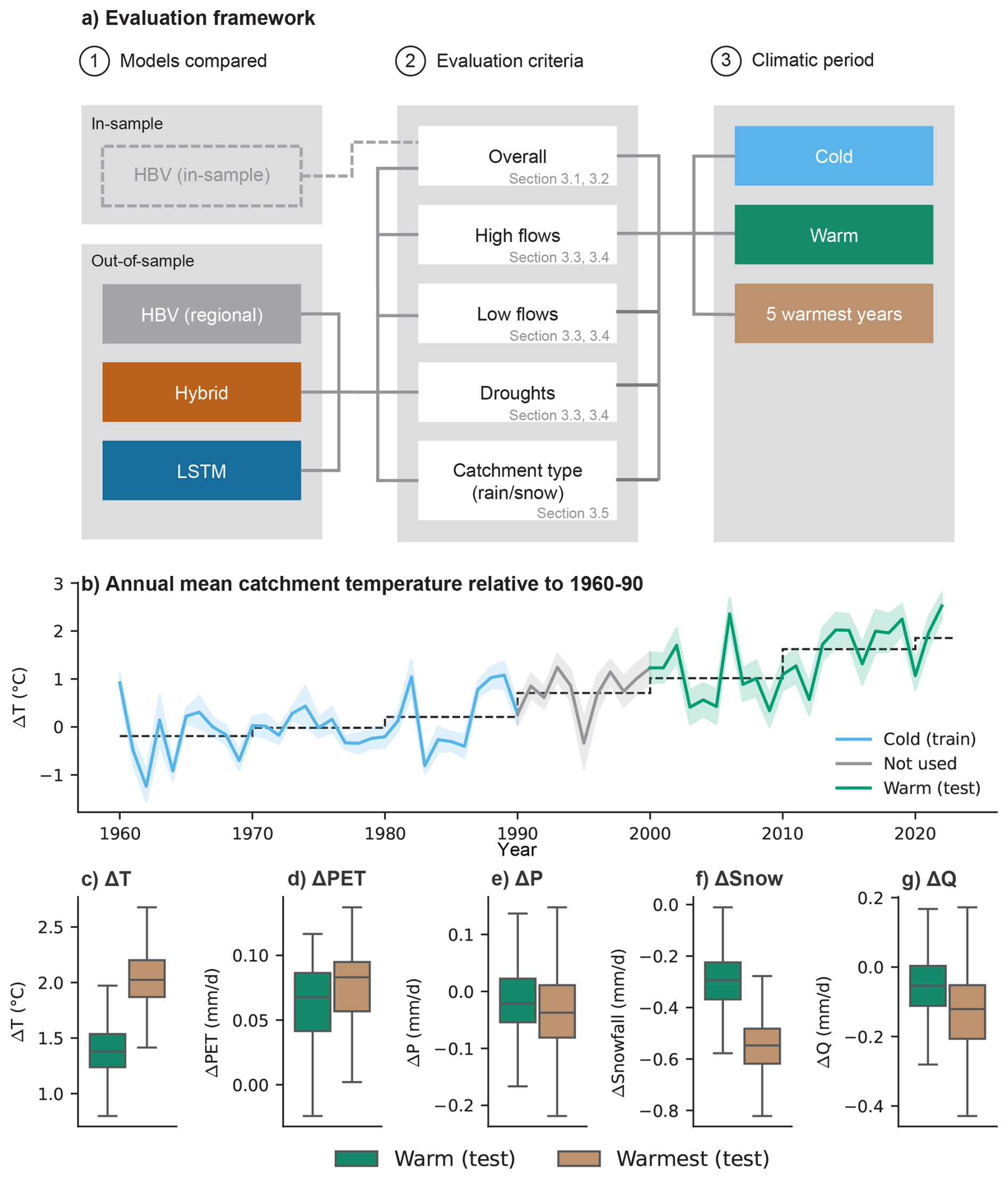
Figure 2Schematic of the evaluation framework and an overview of the climatic conditions in the three evaluation periods considered. (a) Overview of the different models, evaluation criteria and climatic periods used. (b) Evolution of the yearly mean temperature relative to the 1960–1990 mean for each catchment, with the line indicating the mean over catchments and the shaded area representing the standard deviation in each direction. The colors indicate the cold and warm period. The dashed lines indicate the decadal mean temperature relative to the 1960–1990 mean averaged over all catchments. (c–g) Climatic conditions during the warm and warmest evaluation period compared to the cold training period. The warmest period is defined as the 5 warmest years for each basin. For each variable, the catchment average of the cold period is subtracted from the catchment average of the evaluation periods. The boxes show the interquartile range, with the horizontal line indicating the median. The whiskers indicate the data points furthest away from the first and third quartile but still within 1.5 times the interquartile range from those quartiles. Outliers are not shown for improved readability.
In addition to evaluating general model accuracy, we evaluated the models with respect to how well they simulate extreme events such as peak flows, low flows, and drought events (i.e. seasonal low flow anomalies). Specifically, we considered the following flow metrics for each catchment: the high flow percentage bias (HFPB), the low flow percentage bias (LFPB), and the drought volume percentage bias (DVPB). The HFPB was defined as the percentage bias for days during which the observed streamflow exceeded the observed 99th quantile, that is
where the index t runs over only days with Qt larger than the 99th quantile. The LFPB was defined using the annual minimum flow rate averaged over a 7 d window (NM7Q)
We computed the NM7Q for each hydrological year for the observed and simulated streamflow time series. To obtain a catchment-level metric, we considered the percentage bias of the yearly NM7Qs defined as
with simulated and observed NM7Qy for the hydrological year y. Finally, we considered the DVFP metric based on drought events defined using a seasonally varying threshold approach (Brunner et al., 2023). The observed streamflow data was smoothed by taking running averages and a seasonally varying threshold was determined for each day of the year as the 20th percentile for a 30 d window around that day. This threshold was used to detect drought events as periods during which the observed streamflow lies below the threshold for at least 30 consecutive days. The DVPB for a catchment was then defined as the percentage bias between simulated and observed flow volumes during drought events
where E is the set of drought events detected for that catchment, e is an individual event and are the observed and modelled flow volumes for that event.
As an additional measure of generalizability and to compare the sensitivity of the models, we compared the changes in mean flow, the NM7Q and the annual 99th streamflow percentile between the two testing periods (warm and warmest) and training period (cold) in observations with the simulated change signals by the three models. Further, we calculated catchment-by-catchment differences of these change signals. We tested for significant differences among models with a two-sided sign test.
Next, we compared model accuracy and generalizability for snow- vs. rainfall-dominated catchments across the different model types to assess whether these two aspects depend on the fraction of snowfall. We defined snow-dominated catchments as catchments where snowfall makes up more than 30 % of precipitation (during the cold period) and compared model accuracy in these catchments to the one of rainfall-dominated catchments (less than 30 % snow fraction). Snowfall was defined as precipitation falling on days with air temperatures below 0 °C. We excluded catchments with significant glacier area (larger than 2 % of the total catchment area according to RGI v2.0; RGI Consortium, 2012) from this model evaluation since the HBV and hybrid models do not explicitly account for glaciers. In order to understand potential model differences in terms of model accuracy and generalizability in snow-dominated catchments, we looked at how the HBV and hybrid models represent snow. As the LSTM does not explicitly model SWE, we disregarded this model for this analysis. We compared the snow-water equivalent (SWE) modelled by the HBV and hybrid models to observed SWE values derived from gridded SWE datasets for Austria and Switzerland. We focused on these two countries because there are no gridded observational SWE datasets of comparable quality for France and Germany.
3.1 Model accuracy during the “cold” calibration period
For a general comparison of model performance across the three model types, we first focus on model accuracy in ungauged basins during the cold (training) period (Fig. 3, Table C2). Out of the three models, the LSTM has the highest accuracy, with a median KGE (NSE) of 0.76 (0.79). The hybrid and conceptual regional HBV models show a lower accuracy of 0.72 (0.71) and 0.60 (0.56). The regionalization of the parameters of the HBV model results in a reduction in accuracy by 0.15 (0.10) as compared to the in-sample HBV from a median KGE (NSE) of 0.75 (0.66) to 0.60 (0.56).
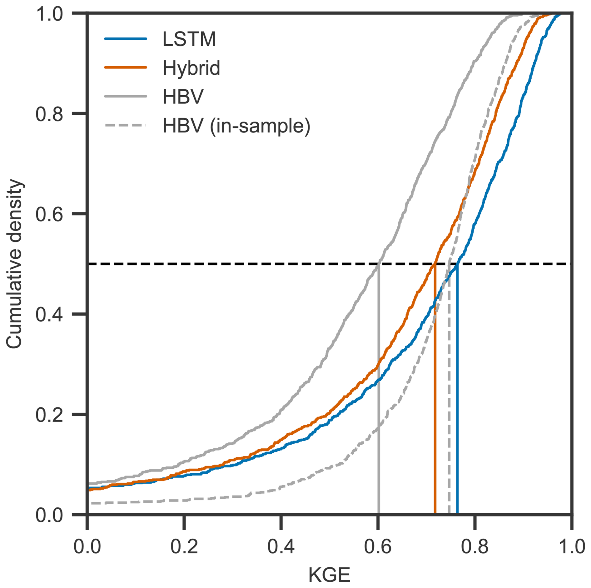
Figure 3Model accuracy comparison during the cold training period for the three model types: (1) data-driven (LSTM), (2) hybrid (δ-HBV), and (3) conceptual (HBV), using the empirical cumulative distribution of the KGE metric. KGE values below 0 are not shown. Solid lines represent models evaluated on catchments not used during training, while the dashed line represents the conceptual model evaluated on catchments in the calibration set. The vertical lines indicate the medians of the KGE distributions per model.
3.2 Model generalizability to periods with warmer climate conditions
To assess how well the different models represent streamflow under warmer conditions, we compare general model accuracy across the three model types in terms of KGE when applying the models under warmer climatic conditions than those observed during training. Model accuracy varies for all models depending on the period considered and decreases more strongly with the degree of extrapolation (Fig. 4a). During the cold period, the LSTM performs significantly better than the hybrid model (p value <0.05 for a one-sided sign test). It also performs significantly better than the HBV model during all periods. For the extrapolation periods (warm and warmest), the difference in accuracies between the LSTM and hybrid model are statistically insignificant (p value >0.05 for both alternatives of the one-sided sign test). At the same time, the hybrid model has a significantly higher accuracy than the HBV model in all periods.
To compare the generalizability of the three models, we now investigate the per catchment change in accuracy between the cold period and the two extrapolation periods (warm and warmest; Fig. 4b). The LSTM shows a large median change in KGE (NSE) −0.05 (−0.03) when evaluating it on the warm instead of the cold period, while the hybrid and HBV models show a smaller and similar change of −0.02 (0.00) and −0.02 (0.00). This results in median KGE (NSE) scores of 0.71 (0.75) for the warm period for the LSTM, 0.70 (0.71) for the hybrid model, and 0.58 (0.54) for the conceptual HBV model evaluated in ungauged basins. Considering only the 5 warmest years in each catchment leads to even stronger accuracy reductions with respect to the cold period. These are again strongest for the LSTM as compared to the other models, with changes of −0.06 (−0.04) in the KGE (NSE) for the LSTM and of −0.03 (−0.02) and −0.02 (−0.01) for the hybrid and conceptual models, respectively. For this warmest period, the median KGE score of the hybrid model approaches that of the LSTM (0.69 for both), indicating that they both perform equally well under strong extrapolation in terms of absolute accuracy. While the change in accuracy of the regional HBV model is similar to that of the hybrid model, its absolute accuracy (KGE of 0.56) still lies clearly below the one of the LSTM (KGE of 0.69). Even though it generalizes well, the HBV model still has a lower absolute accuracy during extrapolation to very warm conditions than both types of deep learning models. The change in accuracy is not significantly different between the HBV and hybrid models (p value >0.05 for a two-sided sign test) for both periods, while there is a significant difference between the change in accuracy of the LSTM and that of the other two models (p value <0.05 for a two-sided sign test). The accuracy of the in-sample HBV model is comparable to that of the LSTM and hybrid models for the warm and warmest periods with a median KGE (NSE) score of 0.69 (0.63) and 0.68 (0.61), respectively (see Table C2). In terms of generalizability, the in-sample HBV shows a larger reduction in accuracy between the cold period and the extrapolation periods than the HBV and hybrid models, with a median change in KGE (NSE) of −0.05 (−0.02) and −0.05 (−0.03) for the warm and warmest period respectively. This is comparable to the change in KGE (NSE) of the LSTM model.
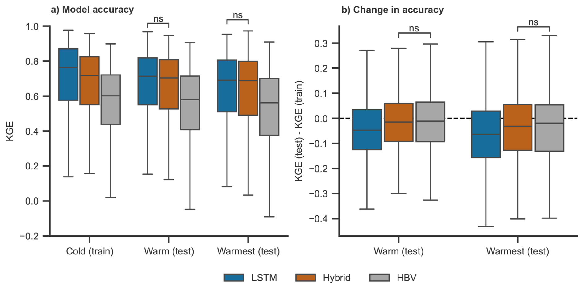
Figure 4Model accuracy during periods with different climate conditions for the three model types: (1) data-driven (LSTM), (2) hybrid (δ-HBV), and (3) conceptual (HBV). (a) KGE for the cold, warm, and warmest periods across catchments and (b) change in KGE between the warm and warmest periods and the cold period across catchments. For the conceptual HBV model, only the evaluation in ungauged basins is shown. The boxes show the interquartile range, with the horizontal line indicating the median. The whiskers indicate the data points furthest from the first and third quartile but still within 1.5 times the interquartile range from those quartiles. Outliers are not shown for improved readability. Above the boxplots, we show the results of a one-sided sign test for the absolute KGE values (a) and a two-sided sign test for the change in KGE values (b). The model pairs where the p value is above 0.05 are indicated by “ns”. For all other pairs, significant differences are found.
Looking at the different components of the KGE (Table C2), we find that the change in KGE of the LSTM is largely explained by reductions in the bias and variability terms. The simulations derived with the LSTM and hybrid models most closely match the observed mean flow in the training period, with bias terms βKGE of 0.99 and 1.01 respectively (values above and below 1 indicate an overestimation and underestimation of the mean flow, respectively; see Table C2, Fig. C1 in Appendix C). In the warm period, the bias of the LSTM more strongly increases (βKGE of 0.94), than the one of the hybrid and HBV models (βKGE=0.97). In the warmest period, the hybrid and HBV models but not the LSTM match the observed mean flow even better than in the warm period (bias terms of 0.99, 1.00, 0.95). Considering the median bias across all catchments, the LSTM underestimates the mean flow during the warm and warmest periods by 6 % and 5 %, respectively.
Overall, the LSTM experiences the strongest accuracy reduction between the cold period and the two extrapolation periods among the three model types considered. In absolute terms, the LSTM is more accurate than the regional HBV during extrapolation in all metrics but the bias term (βKGE), while it is on par with the hybrid model with respect to most evaluation metrics. In terms of the NSE metric, the LSTM is the most accurate model in all periods. The three model types do not generalize equally well to warmer climate conditions in all catchments. We find that particularly the hybrid and HBV models generalize less well in catchments with higher mean specific discharge than in catchments with smaller specific discharge (Sect. C1 and Fig. C2a). Such high mean specific discharge is associated with higher elevation catchments with larger snowfall fractions (Sect. C1).
3.3 Model accuracy and generalizability for extreme events
To assess how model accuracy and generalizability for the three model types compare for extreme events, we investigate the ability of the models to represent high and low flows across the three climate periods (Fig. 5, Table C2). In general, all models tend to underestimate flood peaks during the cold training period (Fig. 5a). During this period, the LSTM is more accurate in representing flood peaks than the hybrid model (HFPB of −8.2 % and −11.8 %, respectively). The hybrid model in turn is more accurate than the regional HBV model (−17.7 %) and the in-sample HBV (−13.5 %, not shown in figure). While the LSTM and hybrid model show similar accuracies in the warm period (−13.7 % and −13.3 %), the hybrid model (−10.7 %) has a notably higher accuracy than the LSTM (−13.8 %) in the 5 warmest years. While having a lower accuracy than the hybrid model when extrapolating strongly, the LSTM still has a higher accuracy than the regional HBV during both testing periods, which has percentage biases of −18.5 % and −16.4 % for the warm period and the 5 warmest years, respectively. Similarly, the LSTM has a higher accuracy during extrapolation than the in-sample HBV, which has percentage biases of −15.9 % and −16.6 % for the warm period and the 5 warmest years.
To compare model accuracy and generalizability for low flows, we on the one hand focus on absolute low flows and on the other hand consider drought events representing seasonal flow anomalies. While some model types tend to overestimate low flows, others underestimate them (Fig. 5b–c). The LSTM mostly overestimates absolute low flows with median LFPB of 9.9 %, 8.6 % and 11.8 % for the cold, warm and warmest periods (Fig. 5b). In contrast, both the hybrid and HBV model underestimate low flows with LFPBs for the cold, warm, and warmest period of −12.1 %, −10.9 % and −10.3 % for the hybrid model and −10.0 %, −5.6 %, −5.0 % for the HBV. While the HBV model has a median across catchments closest to zero for the warm and warmest periods, it also has the largest interquartile range of all models for all periods. Considering the median across all catchments, the hybrid and HBV models are thus more accurate at modelling absolute low flows during the warm and warmest period than during the cold period. Similarly, the LSTM also models low flows more accurately in the warm period than in the cold period. For drought events defined as seasonal low flow anomalies, the three model types behave in a more consistent way than for absolute low flows as all of them tend to overestimate streamflow during drought events (Fig. 5c). Among the three model types, the hybrid model has the highest accuracy in all periods with median percentage biases of 9.5 %, 4.9 %, 8.8 % for the cold, warm, and warmest periods. The HBV model can compete with the hybrid model in the cold period, but has considerably lower accuracy in the warm and warmest periods with median DFPB of 8.8 %, 10.9 % and 15.5 %. The LSTM is the least accurate model in the cold period, but performs better than the HBV model in the warm and warmest periods with percentage biases of 10.4 %, 9.1 %, and 9.7 %. Similarly to when considering absolute low flows, the HBV model again shows the largest accuracy spread across catchments among the three models. For droughts, only the regional HBV model shows decreasing accuracy in the extrapolation periods compared to the cold period. The LSTM has similar percentage biases in all periods, while the hybrid model is better at representing droughts in the warm period than in the cold period.
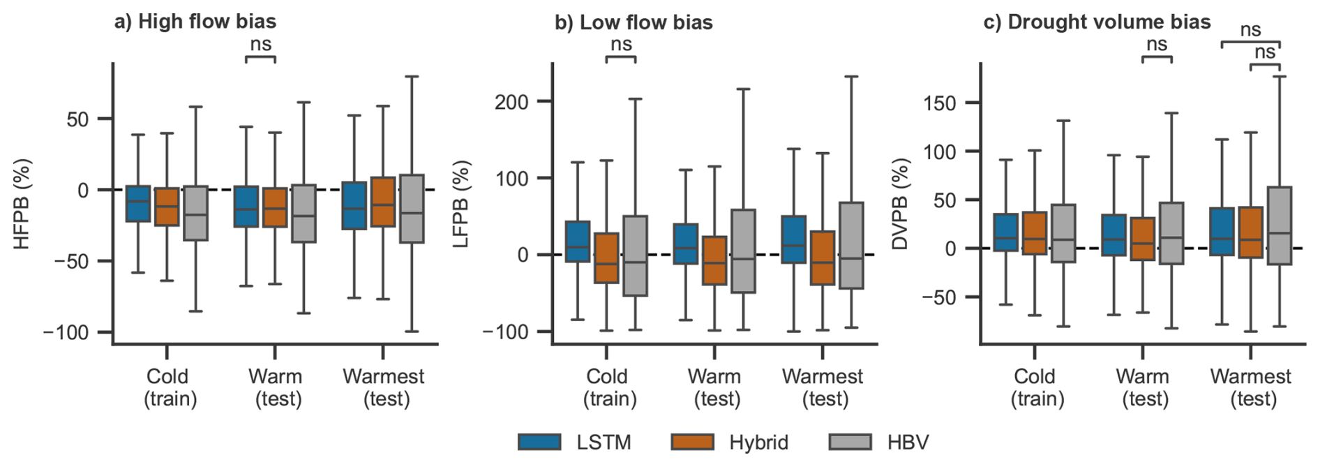
Figure 5Model accuracy comparison for the three model types: (1) data-driven (LSTM), (2) hybrid (δ-HBV), and (3) conceptual (HBV) for different types of hydrological extreme events including (a) high flows (percentage bias for days where streamflow exceeds the observed 99th quantile), (b) absolute low flows (percentage bias in the yearly NM7Q), and (c) seasonal low flow anomalies, i.e. droughts (volume percentage bias for detected drought events). For the conceptual HBV model, only the evaluation in ungauged basins is shown. The boxes show the interquartile range, with the horizontal line indicating the median. The whiskers indicate the data points furthest from the first and third quartile but still within 1.5 times the interquartile range from those quartiles. Outliers are not shown for improved readability. Above the boxplots, we show the results of a two-sided sign test. The model pairs where the p value is above 0.05 are indicated by “ns”. For all other pairs, significant differences are found.
3.4 Model generalizability in preserving trends
Next, we look at generalizability from the perspective of trend preservation. For each catchment, we compare the absolute delta in the change signal between the warm (warmest) and cold period simulated by the models to the one derived from observations. Good generalizability is given when models capture the magnitude and direction of change detected in observations, both at regional and catchment scale. Overall, observations show a decreasing trend in daily mean streamflow (MQ) in the warm period compared to the cold period (−4.6 %), with even stronger decreasing signals for the warmest years (−9.4 %) (see Fig. 6a). All models are able to capture the overall decreasing trend in MQ in the region, and all show a stronger signal in the warmest compared to warm period. The LSTM shows stronger trends in both periods (warm: −8.5 %; warmest: −12.6 %) compared to observations and the other models, and has a median catchment level signal bias of −3.8 % pts in the warm period and −2.8 % pts in the warmest period (Fig. 6d). The Hybrid model overestimates the regional signal in the warm period as well (signal: −7.6 %, bias: −3.0 % pts), but compares well with observations in the warmest period (signal: −10.1 %, bias: −0.2 % pts). The HBV model shows signals in the warm period that are comparable to those in observations (signal: −5.0 %; bias: −0.2 % pts), but slightly underestimates signals in the warmest period (signal: −7.4 %; bias: +2.0 % pts). Similarly, high flows (the mean 99th percentile of daily streamflow in a year) are decreasing in the observations and most catchments (warm: −3.6 %, warmest: −9.7 %; Fig. 6b). Again, all models generally agree with observations on a decrease in high flows, as well as even lower high flows in the warmest period compared to the cold period. In general, the LSTM again overestimates the decreasing streamflow signals in the warm period (signal: −7.0 %, bias: −4.7 % pts) and warmest period (signal: −13.4 %; bias: −5.5 % pts) (Fig. 6b, e). The Hybrid and HBV model show comparable signals to observations in both periods (Fig. 6b) and show catchment level signal biases that are below 1.5 percentage points (Fig. 6d). For low flows (mean annual NM7Q) the observations show a small overall change in the warm period (−1.1 %), but a stronger increase in low flows in the warmest period (−9.2 %; Fig. 6c). In the warm period, the Hybrid model compares best with observed low flow signals followed by the LSTM, while HBV shows slightly positive low flow signals. However, the LSTM shows a considerably lower signal spread across catchments than observations and the other models. In the warmest period, the LSTM shows the best match with observed low flow signals followed by the Hybrid model, while the HBV model shows a considerable positive bias in the signals. From the perspective of trend generalizability, the Hybrid model performs best among the three models followed by the HBV model, with the exception of low flows. The LSTM generally shows the same direction of change as observations, but has a slightly enhanced sensitivity compared to observations and the other models.
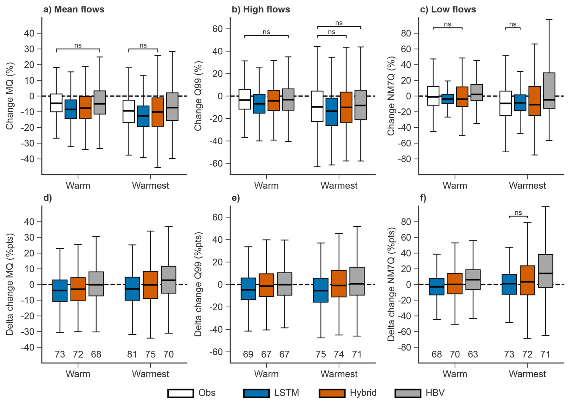
Figure 6Comparison of observed and simulated streamflow trends between the different periods in all catchments. (a–c) Relative differences in (a) mean flow (MQ; mean annual streamflow), (b) high flows (Q99; mean 99th percentile of daily streamflow in a year), and (c) low flows (NM7Q; mean annual NM7Q) between the warm/warmest and cold period. (d–f) Catchment-wise differences in the (d) mean flow, (e) high flow and (f) low flow signals between the model and observations. Above the boxplots, we show the results of a two-sided sign test. The model pairs where the p value is above 0.05 are highlighted by “ns”. For all other pairs, significant differences are found. Below the boxplots in (d)–(f), we show the model agreement with observations, that is the percentage of catchments with an agreement on the sign of change.
3.5 Model generalizability in snow- vs. rainfall-dominated catchments
As previously mentioned, the hybrid and HBV models generalize worse in catchments with large mean specific flows than in catchments with lower specific flows (Sect. C1 and Fig. C2). The catchments with large specific flows are often located at high elevations and strongly snow influenced. Since both types of models explicitly parametrize snow, the question arises how such models generalize to warmer climatic conditions in snow-influenced catchments compared to the purely data-driven LSTM model, which does not explicitly represent snow. To address this question, we compare the model simulations of the three model types for snow-dominated and rainfall-dominated catchments in terms of general model accuracy described by KGE (Fig. 7a–b). During the cold period, the accuracy of all three model types does not differ between the two groups of catchments. That is, model accuracy is as good for snow-dominated catchments as it is for the rainfall-dominated ones. Across both types of catchments, the LSTM performs best out of all models, followed by the hybrid and the HBV model. Notable is the larger spread in the interquartile range of the hybrid model across snow-dominated vs. rainfall-dominated catchments. For snow-dominated catchments, the pattern persists for the two extrapolation periods, i.e. the LSTM keeps showing significantly higher accuracy than the hybrid and regional HBV models (p value <0.05 for the one-sided sign test). For rainfall-dominated catchments, the hybrid model is on par with the LSTM similarly to the previous observations for all catchments combined (p value <0.05 for the cold period and p value >0.05 for the warm period and 5 warmest years) (Fig. 7). The LSTM is still significantly more accurate than the HBV for all periods in rainfall-dominated catchments (p value <0.05).
In contrast to absolute accuracy, the per catchment change in accuracy between the cold period and the two extrapolation periods shows clear differences between snow- and rainfall-dominated catchments. For snow-dominated catchments, all models exhibit a similar reduction in accuracy when extrapolating to warmer climate conditions (Fig. 7c, p value >0.05 for all combinations in the two-sided sign test). In contrast, the accuracy reduction during extrapolation depends on the model for rainfall-dominated catchments. There, the hybrid and the HBV model have a smaller and similar (p value <0.05) reduction in accuracy, while the reduction in KGE of the LSTM is larger and significantly different (p value <0.05) from that of the two other models.
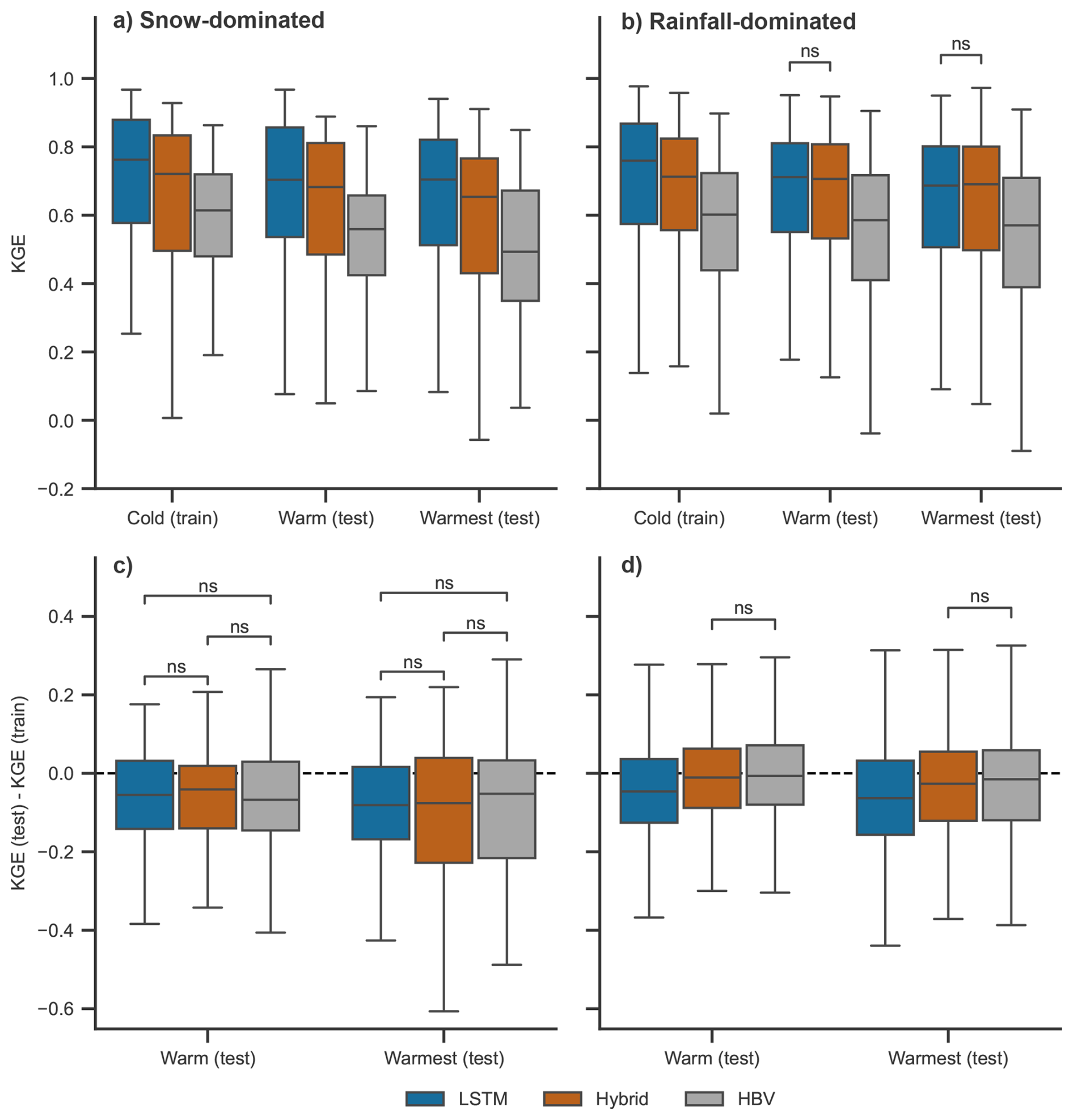
Figure 7Comparison of model accuracy in terms of KGE in (a) snow- vs. (b) rainfall-dominated catchments for the three model types: (1) data-driven (LSTM), (2) hybrid (δ-HBV), and (3) conceptual (HBV). Change in KGE between the warm and warmest periods and the cold period for (c) snow-dominated and (d) rainfall-dominated catchments. For the conceptual HBV model, only the evaluation in ungauged basins is shown. The boxes show the interquartile range, with the horizontal line indicating the median. The whiskers indicate the data points furthest from the first and third quartile but still within 1.5 times the interquartile range from those quartiles. Outliers are not shown for improved readability. The results of a sign test comparing the models within the same periods are shown above the boxplots. Only the model pairs where the results were insignificant (p value >0.05) are shown. All other pairs show significant differences in distributions.
To assess the seasonality of the observed and modelled streamflow regimes in snow-dominated catchments, we consider the discharge averaged by day of the year. We find that the model bias has a distinct seasonal pattern with both the HBV and hybrid model underestimating streamflow during the snowmelt season (April–July) in all periods (Fig. 8). The LSTM accurately models the annual streamflow curves during the cold and warm periods, but it underestimates summer flow during the 5 warmest years (Fig. 8c). This is also reflected in the bias metrics. The hybrid and HBV models underestimate mean streamflow by 14 % and 24 % in snow-dominated catchments during the warm period, while the LSTM only shows an underestimation of 7 % (Table C3), with similar bias values for the warmest periods.
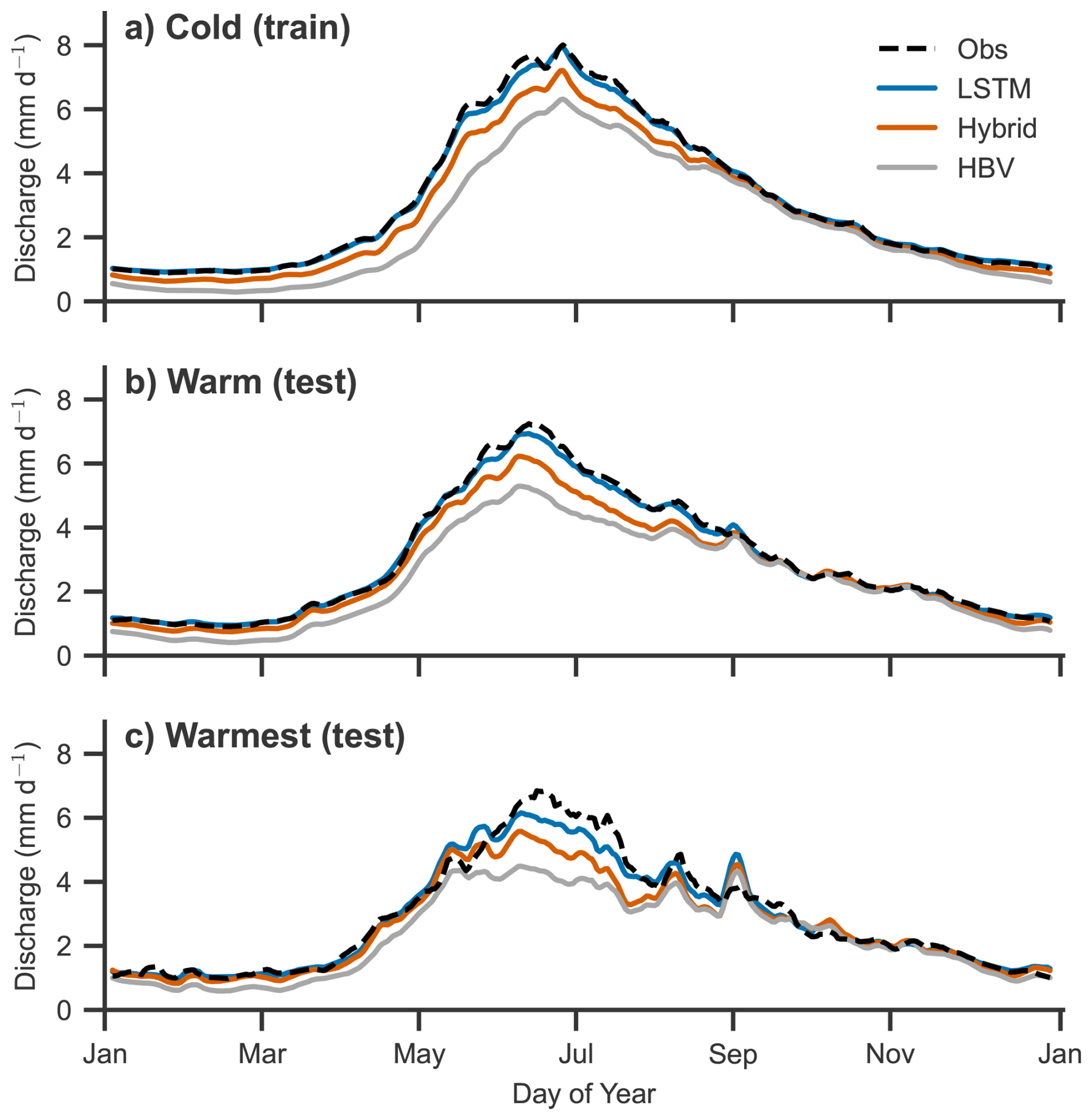
Figure 8Seasonal average streamflow regimes in snow-dominated catchments (more than 30 % snowfall fraction) with little glacier influence (less than 2 % glacier cover) predicted by the three model types: (1) data-driven (LSTM), (2) hybrid (δ-HBV), and (3) conceptual (HBV) for periods with different climate conditions: (a) cold, (b) warm and (c) warmest 5 years. For the conceptual HBV model only the evaluation in ungauged basins is shown.
To further assess the issue of the hybrid and HBV model in terms of flow estimation during the melt season, we look at the internal snowpack variable of these models. Specifically, we compare the SWE simulated with these two models to catchment averages derived from gridded SWE benchmark datasets (OSHD-CLQM in Switzerland and SNOWGRID in Austria). Both models simulate similar SWE estimates and underestimate snowpack throughout the year, both in Swiss and Austrian catchments (Fig. 9). To quantify this SWE underestimation effect, we compute the same metrics also used to evaluate streamflow for simulated SWE (Table C5) and find that the hybrid and HBV models underestimate the mean SWE by 24 % and 22 % respectively in the cold period. The degree of underestimation increases during extrapolation from the cold to the warm periods, with the hybrid model underestimating the mean by 26 % and 33 % for the warm and warmest periods and the HBV model underestimating it by 27 % and 37 %. Both regional models have lower bias than the in-sample HBV model in all periods.
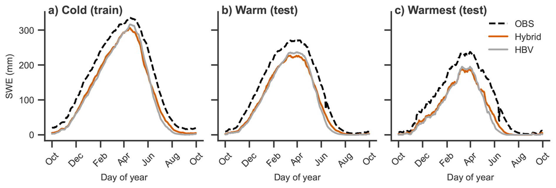
Figure 9Snow-Water-Equivalent simulations by the (1) hybrid (δ-HBV) and (2) conceptual (HBV) model over the three climatic periods: (a) cold, (b) warm, and (c) warmest. SWE was averaged by day of the year for snow-dominated catchments (more than 30 % snowfall fraction) with little glacier influence (less than 2 % glacier cover) in Switzerland (12) and Austria (49). For the conceptual HBV model, only the evaluation in ungauged basins is shown. Please note that the LSTM is not shown because it does not produce any explicit SWE simulations.
4.1 Hybrid models effectively balance the accuracy-generalizability trade-off
Our results show that the LSTM is clearly the most accurate model in terms of modelling streamflow in ungauged basins, i.e. basins lacking streamflow observations for model training (Fig. 3). However, it suffers from poor generalizability under changes in climate (Fig. 4). This finding is consistent with findings of prior studies which have also found larger accuracy reductions for LSTMs than for conceptual models when evaluating them under climate conditions different from those used during training (Bai et al., 2021). In contrast, the hybrid model shows better generalizability, which comes at the cost of slightly reduced accuracy when evaluating it under climate conditions more similar to those of the training period. These results align with previous research showing that hybrid models are better at generalizing to climatic zones not used in training compared to a stand-alone LSTM (Feng et al., 2023, 2024). The regionalized conceptual model is significantly less accurate than the other two models (Fig. 4a). However, the conceptual model shows a small reduction in accuracy similar to the one of the hybrid model, which indicates a similar generalizability to warmer climate conditions as the one of the hybrid model (Fig. 4b). The hybrid model thus effectively combines the strong performance of the LSTM when predicting in ungauged basins with the generalizability of the conceptual HBV model. In years that are +1.4 °C warmer than the average temperature of the cold period, the hybrid model has an accuracy that is indistinguishable from the one of the LSTM. The LSTM, while not generalizing as well as the hybrid and HBV model, still has a significantly higher accuracy than the HBV model even in the warmest period (+2 °C). The lower generalizability of the LSTM compared to the hybrid and HBV model also holds when comparing observed and simulated streamflow signals. The LSTM simulations show a higher sensitivity to changes in meteorological forcings than observations (Fig. 6), that is stronger declines in mean and high flows. This might indicate that when moving to even warmer climate conditions, such as future climate projections, the LSTM might project different streamflow changes differently than the other models. A higher streamflow sensitivity to temperature changes by the LSTM compared to conceptual models has previously also been shown by Martel et al. (2025).
The finding that the LSTM is the most accurate model during the training period, while the hybrid model generalizes best to warmer conditions than those used in training, also holds for extreme events. Our results show that the LSTM most accurately models floods and absolute annual low flows during the training period (Fig. 5a–b). In contrast, all models have similar but lower accuracy for drought deficits, with the hybrid model being the most accurate of the regional models (Fig. 5c). Differences in model accuracies for floods and droughts are common in hydrological modelling irrespective of the objective function used for training (Muñoz-Castro et al., 2026) and model performance often deteriorates under drought conditions (Bruno et al., 2024). The finding that the LSTM is more accurate in ungauged basins than the hybrid model when considering extreme events is in line with previous research (Feng et al., 2023). When generalizing to warmer climate conditions, however, the hybrid model most accurately models floods and drought volumes, while the regional HBV model most accurately models annual low flows. Under these warmer conditions, the hybrid model not only equals the absolute accuracy of the LSTM in extrapolation but even surpasses it. The LSTM in turn models floods more accurately than both the in-sample and the regional HBV model and has lower drought volume bias than the regional HBV. The regional HBV model does not just show lower accuracy than the other two models in terms of most metrics, it also shows a large spread in the distribution of the extreme event metrics, indicating large accuracy differences between different catchments. This is in line with findings from Feng et al. (2023), who show that hybrid models have a smaller percentage bias when simulating peak flows in climatic regions withheld from the training set.
While model generalizability varies across model types when considering all catchments (Fig. 4), the models show similar generalizability in snow-dominated catchments (Fig. 7c). In these catchments, the LSTM has the highest absolute accuracy during the cold period and is also the most accurate model in all periods. Similarly, Feng et al. (2024) have found LSTMs to outperform hybrid models in cold and polar climates. This contrasts with rainfall-dominated catchments, where the HBV and hybrid model generalize significantly better than the LSTM to periods with warmer climate conditions (Fig. 7). These findings suggest that an explicit parametrization of snow and other processes does not always improve generalizability and that process-based approaches can have their own problems under distribution shifts of input variables. Our investigation of simulated SWE for the hybrid and HBV models revealed that both types of models systematically underestimate the water content of the snowpack (Fig. 9). This indicates that there are biases in the forcing data and/or that the models are parametrising snow in a suboptimal way. Precipitation undercatch is one form of bias which is particularly prevalent in snow-dominated catchments (Goodison et al., 1998). While the LSTM can correct for such biases (Fig. 8, Frame et al., 2023), the hybrid and HBV models cannot (Figs. 8, 9). This could be an explanation for the underestimation of SWE and summer streamflow in snow-dominated catchments observed in the hybrid and HBV models (Figs. 8, 9). HBV models calibrated for a specific site often have a snowfall correction factor to account for this type of bias, but such a factor is difficult to regionalize (Beck et al., 2016) and was therefore not included in the conceptual models used in this study. To still account for undercatch, one could directly correct observational precipitation data before feeding it into the hydrological model (Meyer et al., 2019).
4.2 Implications for climate change impact studies
Our findings show that both types of deep learning models (purely data-driven LSTM and hybrid model) achieve the same accuracy in ungauged basins as the in-sample HBV model, even when extrapolating to warmer climatic conditions. Together with their strong ability to extrapolate to ungauged regions, these findings highlight the potential of data-driven and hybrid models for climate change impact assessments in data-scarce regions. The promise of deep learning streamflow models extends to gauged basins because LSTMs and hybrid models have even higher absolute accuracy when evaluated in the catchments they were calibrated in Feng et al. (2023, 2024). The strengths of LSTMs and hybrid models extend from general streamflow simulations to extreme events, i.e. high flows and annual low flows (Fig. 5). This is crucial for climate change impact assessments since hydrological extreme events such as floods are among the most prevalent natural disasters (UNDRR and CRED, 2020), particularly affect low- and middle-income countries (Rentschler et al., 2022), and are already changing in response to increasing temperatures (Dai, 2013; Berghuijs et al., 2019; Bertola et al., 2020). Our results thus suggest that deep learning based models, in particular hybrid models, should be considered as an alternative to conceptual models for climate change impact assessments. In snow-dominated catchments, the stand-alone LSTM can also be considered due to its higher absolute accuracy (Fig. 7). It is important to note, that in contrast to conceptual and hybrid models, the LSTM does not directly provide insights into the processes generating its predictions. This would be needed though to attribute changes in streamflow simulations to changes in underlying processes. For this purpose, hybrid models have an advantage because they directly provide access to variables the model has not been trained on such as snowpack, with comparable quality as conceptual models (Fig. 9, Feng et al., 2022a, 2023, 2024).
Improving the generalizability of data-driven models is an area of active research, and different techniques have been proposed to achieve this (Liu et al., 2023). Hybrid modelling is one possible approach (Vasudevan et al., 2021), which is confirmed by our results. Further, model generalizability could be improved by including catchments from regions whose climate is warmer than that of the region of interest as additional training catchments for deep learning based models (Martel et al., 2025). This allows these models to learn from a more diverse set of climates, which could help improve generalizability. Studies testing this approach on LSTMs have found that such geographically extended models can provide more realistic projections under climate sensitivity analyses than regional LSTMs (Wi and Steinschneider, 2022, 2024). Testing this approach with realistic climate scenarios in the DSST framework could be an interesting avenue of further research. Other studies have also found improved generalizability when adding conservation of mass requirements to LSTMs (Wi and Steinschneider, 2022, 2024). Further ideas include modifying the training procedure to optimize for worst-case accuracy across different domains (Krueger et al., 2021; Kuhn et al., 2024) and modifying the loss function to optimize for time invariant residuals, a concept derived from causal inference (Peters et al., 2016). It has been demonstrated that the use of such a loss function can improve the generalizability of a conceptual hydrological model under certain circumstances, but comes at the cost of reduced accuracy (Astagneau et al., 2026).
4.3 Limitations
As other model comparison studies, our study faced some challenges and limitations including limited observational data availability and the need to make some modelling choices. Modelling choices e.g. included the choice of an objective function for model training and evaluation. We chose NSE for model training, meaning that we put more emphasis on high flow rather than low flow accuracy (Thirel et al., 2024). To improve the model simulations for low flows, streamflow transformations (Thirel et al., 2024) or modified objective functions (Fowler et al., 2018b) could be used. Another important model choice was the choice of the conceptual model used both for stand-alone modelling and integration into the hybrid framework. We used a model with a snow module relying on a relatively simple degree-day factor, which may not be the optimal choice for simulating streamflow under climate change in snow-dominated catchments (Carletti et al., 2022). Wi and Steinschneider (2024) have also shown that using temperature-based PET methods in conceptual models can result in unrealistic water losses under temperature perturbations of +4 °C, compared to when using a more realistic energy-budget-based PET method. This suggests that the parametrizations of hydrological processes in conceptual models can lead to inaccurate extrapolation when these models are included in a hybrid modelling framework. How exactly the choice of hydrological model and the complexity of the snow module affects the generalizability of the hybrid model remains to be investigated in future studies. For example, one could investigate whether the snow module modifications proposed by Girons Lopez et al. (2020), switching to an energy-based snow module (Warscher et al., 2013; Willkofer et al., 2020) or calibration against snow observations (Finger et al., 2015; Janzing et al., 2025) can further improve the generalizability of hybrid and conceptual models in snow-dominated catchments.
Testing the ability of hydrological models to predict streamflow under changing climatic conditions is challenging due to the lack of ground truth observations and benchmark models. To address this challenge, we used the differential split sample test (DSST; Klemeš, 1986; Seibert, 2003; Coron et al., 2012). While providing insights into model generalizability, this approach limits the assessment of model generalizability to historically observed climate change. To overcome this limitation, other approaches to assess the suitability of hydrological models for climate change impact studies have been proposed. The robustness assessment test (Nicolle et al., 2021; Santos et al., 2025) can be used to check whether biases in the model depend on the properties of the climate input data used for the simulations. Metamorphic testing; Reichert et al., 2024) defines the expected qualitative response of a system to changes in the input data and tests the model's ability to replicate theses responses. This allows for the assessment of the responses of hydrological models to arbitrary changes in the input data, but is limited by current scientific understanding of the hydrological response to changes in climatic variables and can only make qualitative statements about the predictions (Reichert et al., 2024). Both methods – the robustness assessment test and metamorphic testing – could be used to further explore the generalizability of data-driven and hybrid models to warmer climate conditions.
In this study, we used the differential split sample test to assess the accuracy and generalizability of hybrid rainfall-runoff models, fully data-driven, and conceptual models under changing climate conditions. Our results highlight that the model with the highest accuracy in a spatial regionalization context is not necessarily the one with the best generalizability to warmer climate conditions than those seen during model training. Among the three model types considered, the LSTM shows the highest accuracy, while the hybrid model generalizes best under changing meteorological forcings. That is, it shows the lowest drop in performance between periods with different temperature conditions and good agreement with observed streamflow changes. Although the LSTM model does not generalize as well as the hybrid and HBV models, it still performs well in absolute terms even during periods with climate conditions up to 2 °C warmer than those considered for training. The main finding that hybrid models combine high accuracy with satisfactory generalizability – thereby best addressing the accuracy-generalizability trade-off – holds for both streamflow in general (i.e. in terms of KGE) as well as for extreme events including high flows, absolute lows flows, and seasonal low flow anomalies. However, this finding is not universally applicable as snow-dominated catchments (>30 % snow fraction) show a slightly different behaviour in terms of model generalizability than rainfall-dominated catchments. In contrast to rainfall-dominated catchments, where hybrid and HBV models generalize best, all models show equally large accuracy reductions when extrapolating to warmer climate conditions for snow-dominated catchments. We conclude that hybrid modelling is an approach that balances the accuracy-generalizability trade-off by leveraging the strengths of both conceptual (generalization in time) and deep learning models (generalization in space). Therefore, they are a powerful tool for hydrological climate change impact assessments, particularly in ungauged basins where no streamflow observations are available for model calibration.
Table A1Static catchment attributes passed to the LSTMs both in the stand-alone LSTM as well as in the δ-HBV hybrid model.
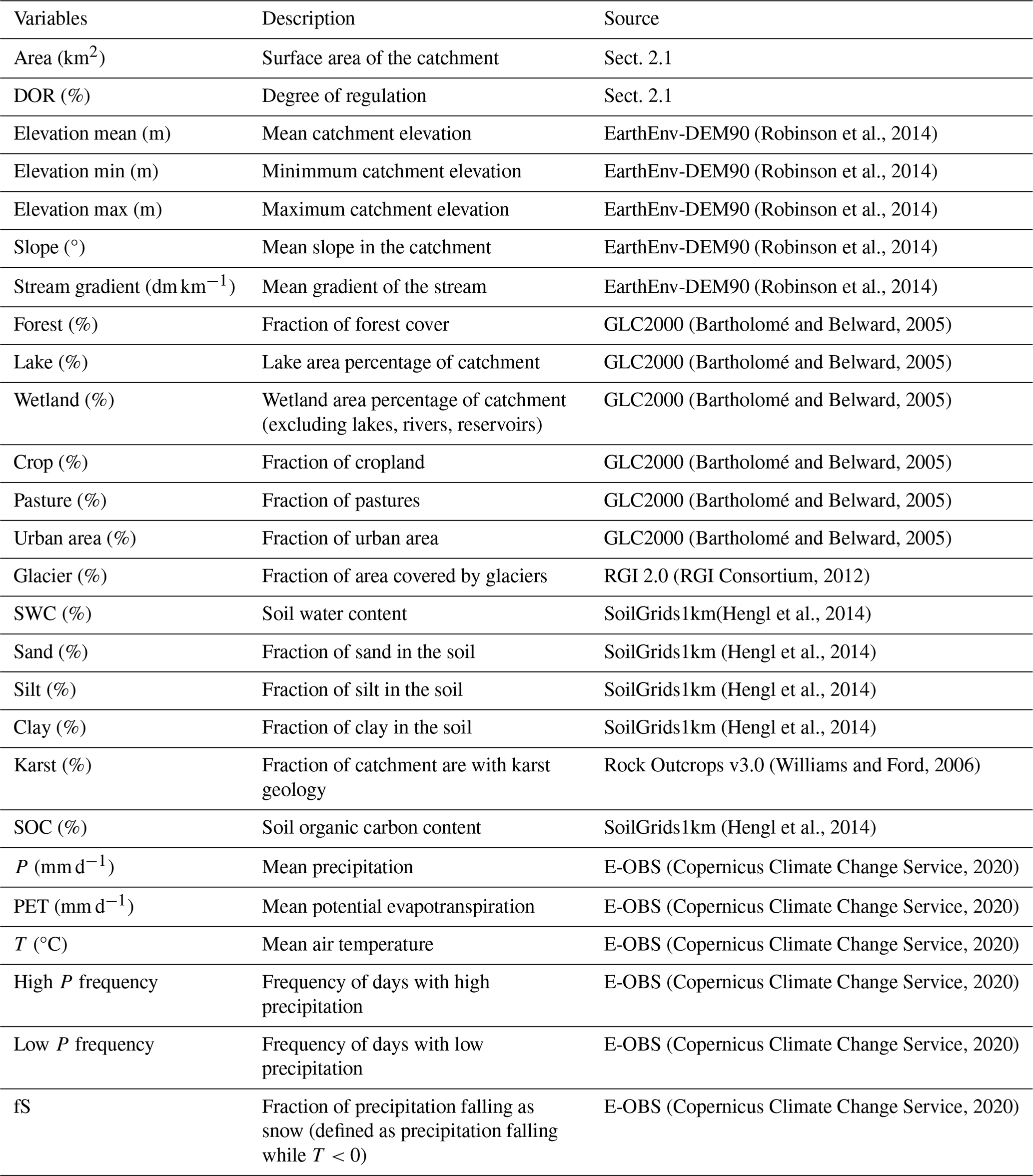
Table A2Meteorological variables passed to the hydrological models. The variables marked with a * are passed to the conceptual HBV model as well as the HBV components of the hybrid model, while the stand-alone LSTM and the LSTM component of the hybrid models also receive the other variables as inputs.
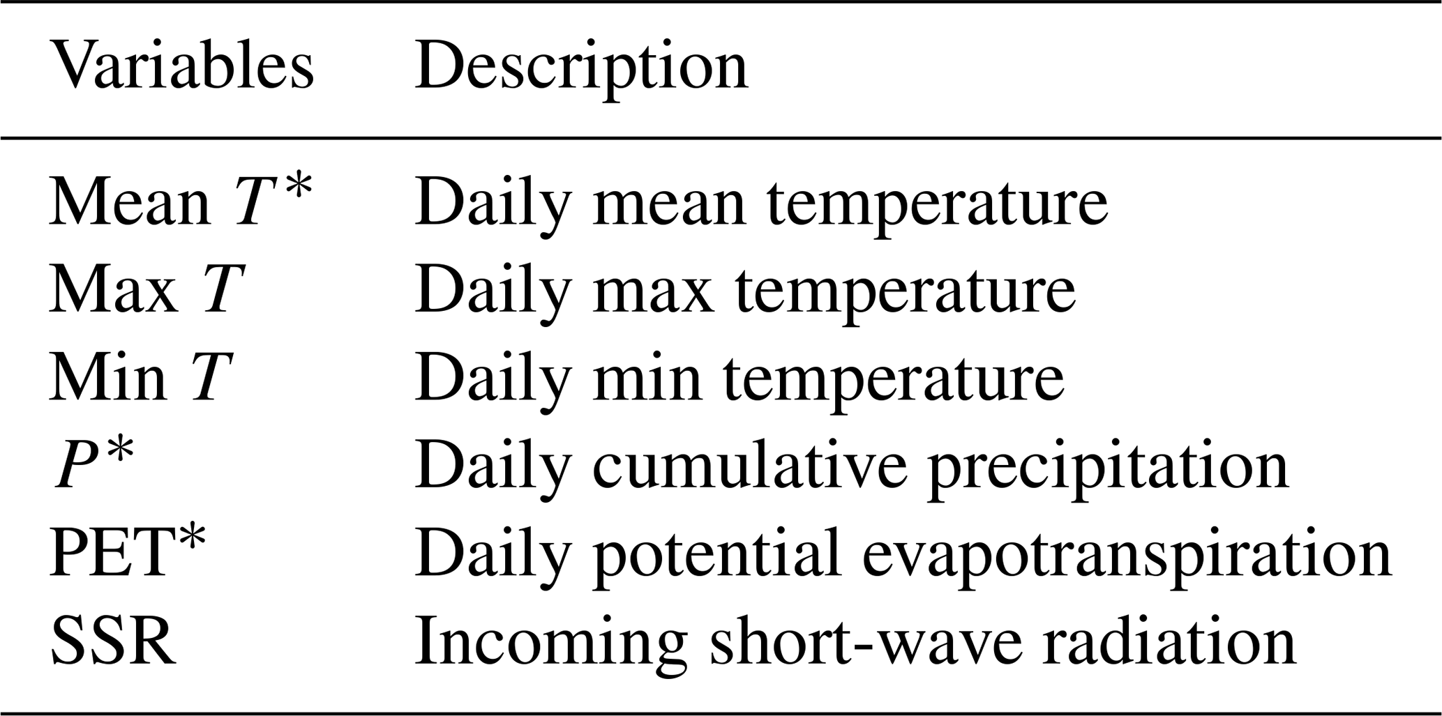
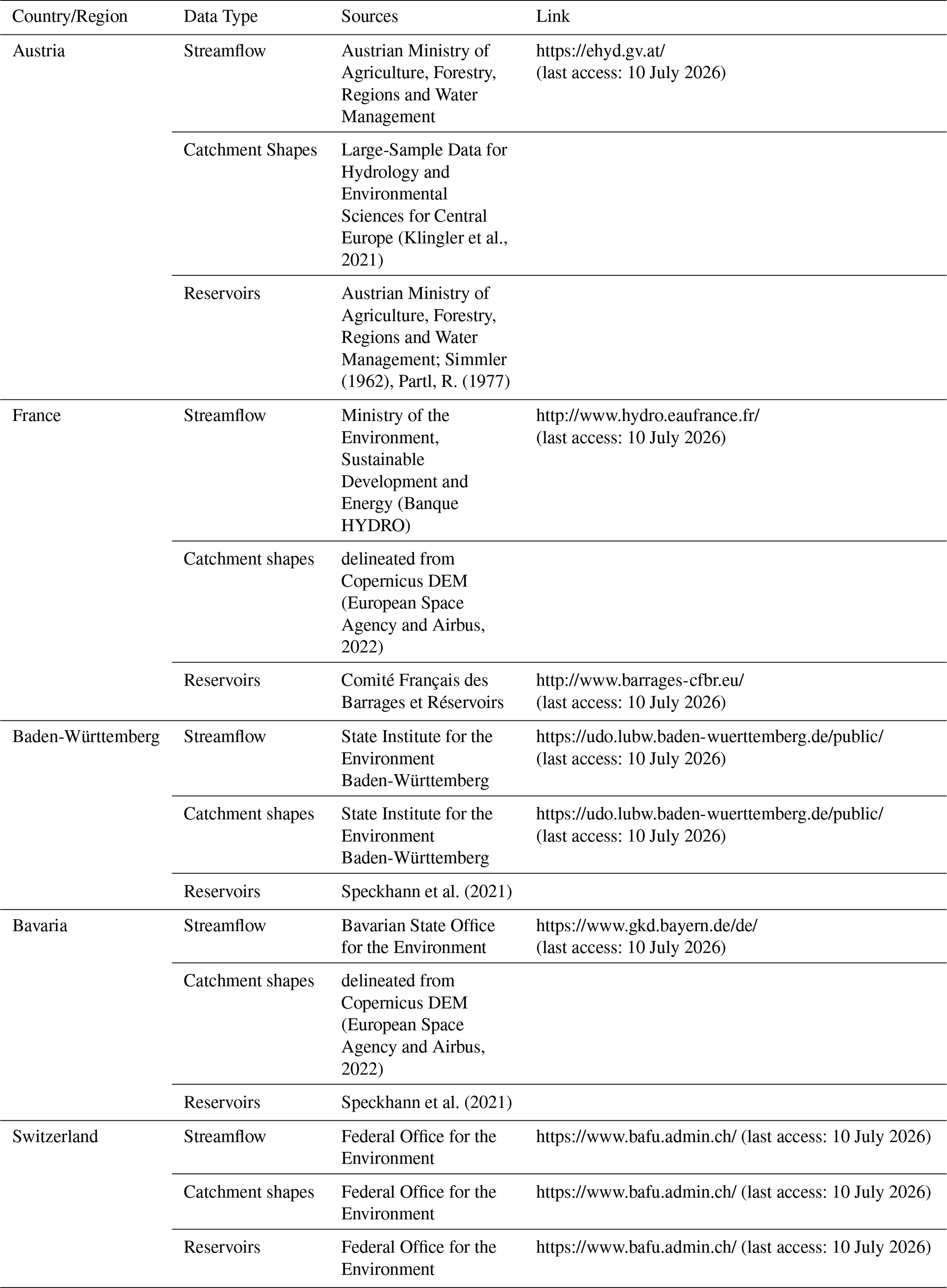
Table A3Sources for the streamflow data, catchment shapes and reservoir data for the different countries.
B1 LSTM
For an input timeseries with xt∈ℝk the model structure of the LSTM is given for all by
with it∈ℝl the input gate, ft∈ℝl the forget gate, gt∈ℝl the potential update vector, ot∈ℝl the output gate, ct∈ℝl the cell state and ht∈ℝl the hidden state. The learnable parameters are the weights and as well as the biases . Here, l is the hidden size of the network and describes the dimension of the latent space, σ is the sigmoid activation function and ⊙ the element-wise multiplication of vectors. For t=0, the cell and hidden states c0 and h0 are usually initialized 0∈ℝl. The crucial step is the update state step of the cell-state ct where the forget gate, which takes values between 0 and 1 is multiplied with the previous cell state ct−1. This rescales the previous cell state and can remove information from previous time steps which is no longer relevant. To this, the element-wise multiplication of the input gate vector with the potential update vector is added. This can similarly be interpreted as choosing the relevant information from the update vector and storing it in the cell state.
B2 HBV parameters and internal states
When analysing the parameters and internal states of the HBV component of the hybrid model, we averaged the quantities over the 16 parallel components and the 5 runs of the ensemble to obtain a single parameter value or state time series per catchments. For the regionalized HBV model, we also averaged both parameters and internal states over the 10 donor catchments.
Table B1Hyperparameters used for the deep learning streamflow models.
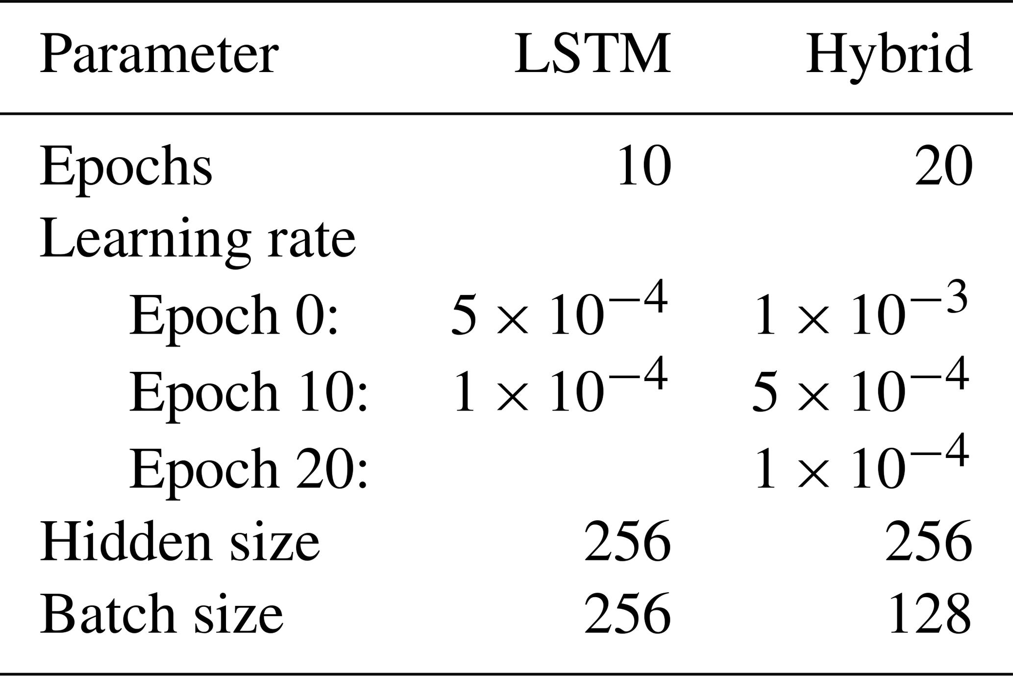
Table B2Variables used to compute catchment similarity for conceptual model parameter regionalization. For each variable, a short description is provided together with the source dataset.
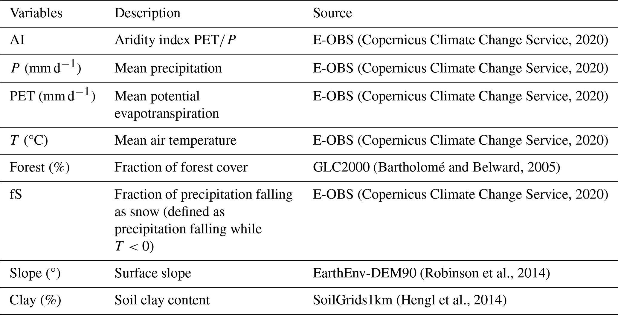
Table C1Evaluation metrics for streamflow and SWE, with representing the observed and simulated mean, representing the observed and simulated variance, and r representing the Pearson-correlation.
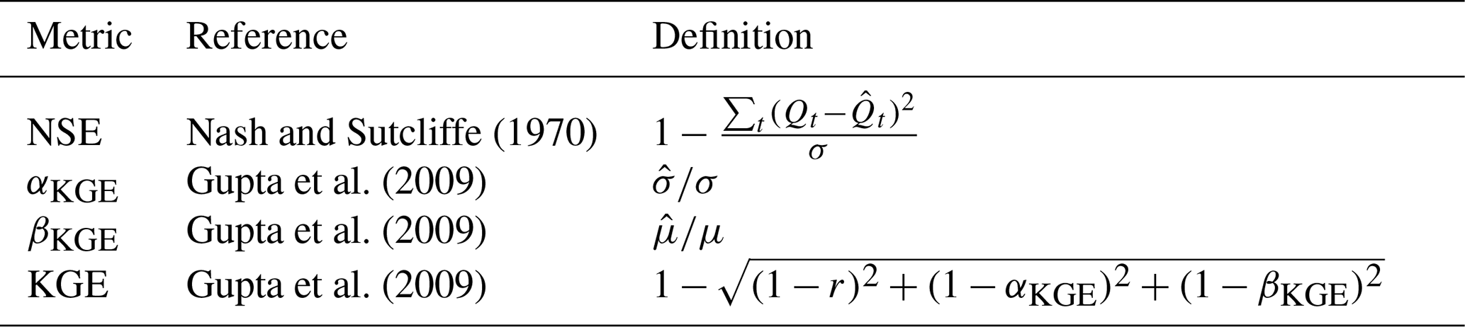
Table C2Streamflow metrics for the three model types: (1) data-driven (LSTM), (2) hybrid (δ-HBV), and (3) conceptual (HBV) for the cold and warm period as well as the 5 warmest years from the warm period in each catchment. The reported value represents the median over all catchments. For each period and metric, the value for the best performing regional model is reported in bold text.
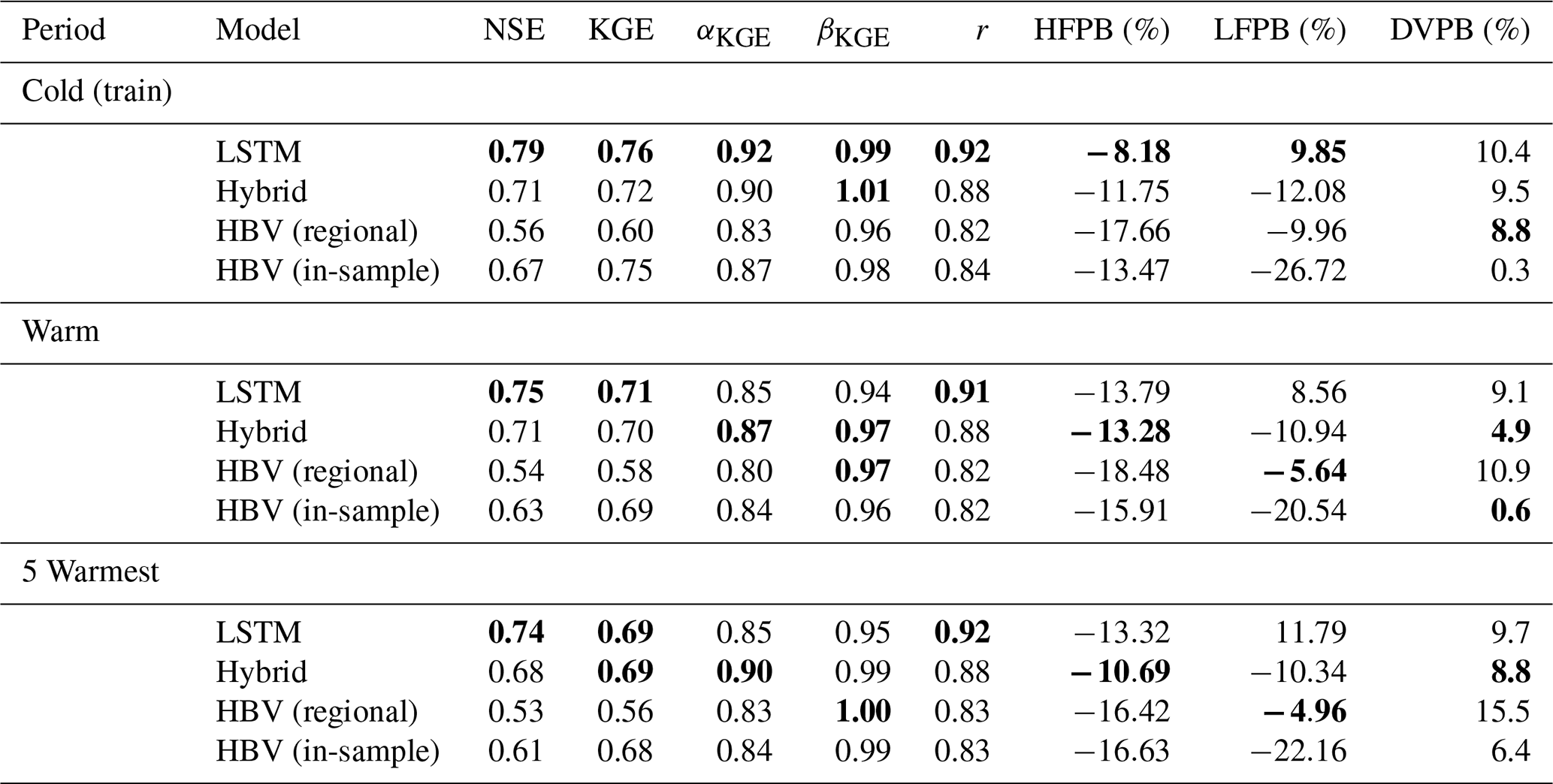
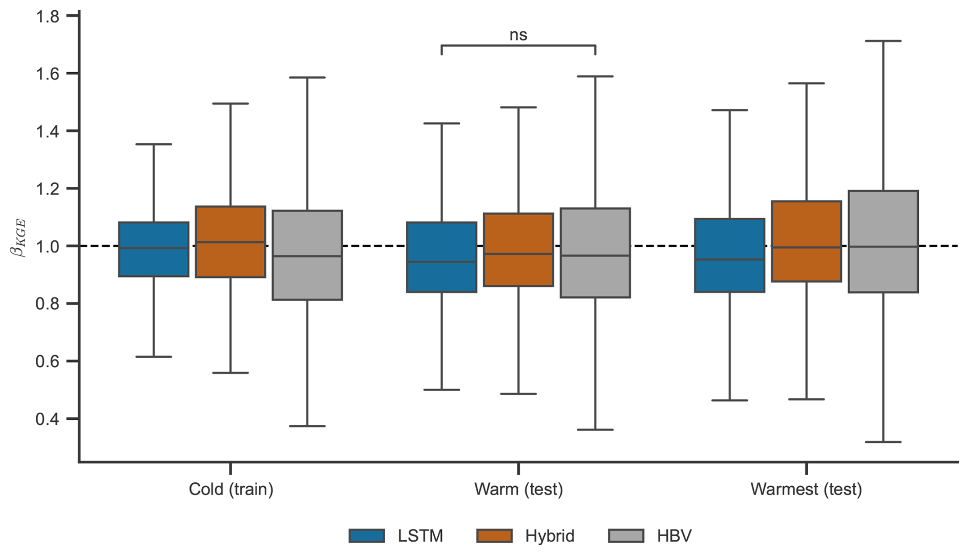
Figure C1Model bias during periods with different climate conditions for the three model types: (1) data-driven (LSTM), (2) hybrid (δ-HBV), and (3) conceptual (HBV). For the conceptual HBV model only the evaluation in ungauged catchments is shown. The boxes show the interquartile range, with the horizontal line indicating the median. The whiskers indicate the data points furthest from the first and third quartile but still within 1.5 times the interquartile range from those quartiles. Outliers are not shown for improved readability.
C1 Feature importance analysis
To determine which static catchment attributes influence the generalizability (defined as the change in KGE between the cold and the warm period) of the models, we trained a random forest regressor for each of the hydrological models. The random forest model received the same static catchment attributes also used to compute the catchment similarity for the HBV regionalization scheme as input, with mean specific discharge and the change in temperature between the cold and warm periods as additional inputs. We then computed the feature importance using the permutation method (Breiman, 2001). The mean specific discharge is clearly the most important feature for predicting generalizability for all hydrological models (Fig. C2a). This feature is positively associated with other features such as elevation (Kendall-τ correlation of 0.54 with p value <0.05) and fraction of snowfall (Kendall-τ correlation of 0.48 with p value <0.05).
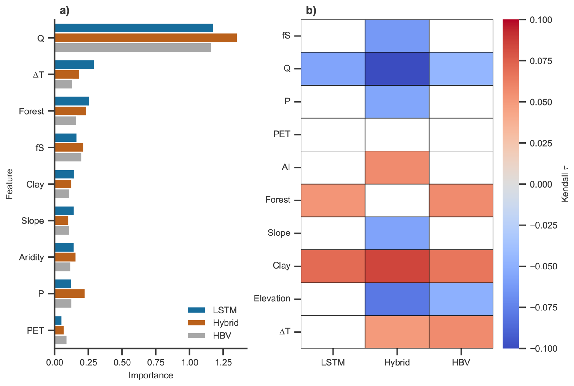
Figure C2Relationship between static catchment attributes and model generalizability for the three model types: (1) data-driven (LSTM), (2) hybrid (δ-HBV), and (3) conceptual (HBV). To determine the relationship between the attributes and generalizability we consider (a) the feature importance of random forest models which learn the relationship between catchment attributes and the generalizability (defined as the change in KGE between the warm and cold period), (b) the Kendall-τ correlation between static catchment attributes and generalization (difference in KGE between warm and cold period). For the conceptual HBV model only the results from ungauged catchments are shown. For panel (a), a larger value indicates that the attribute is a more important predictor. For panel (b), a positive value indicates that as the static attribute increases, the generalizability improves, while negative values indicate the opposite. Only pairs with significant associations (p value <0.05) are shown. The static attributes used for both (a) and (b) are listed in Table B2, with the addition of the mean specific discharge and the difference between the mean temperature during the warm and the cold period.
C2 Model accuracy and generalizability in snow- and rainfall-dominated catchments
Table C3Streamflow metrics during periods with different climate conditions for the three model types: (1) data-driven (LSTM), (2) hybrid (δ-HBV), and (3) conceptual (HBV) in snow-dominated catchments (more than 30 % snowfall fraction) with little glacier influence (less than 2 % glacier cover). For each period and metric, the value for the best performing regional model is reported in bold text.
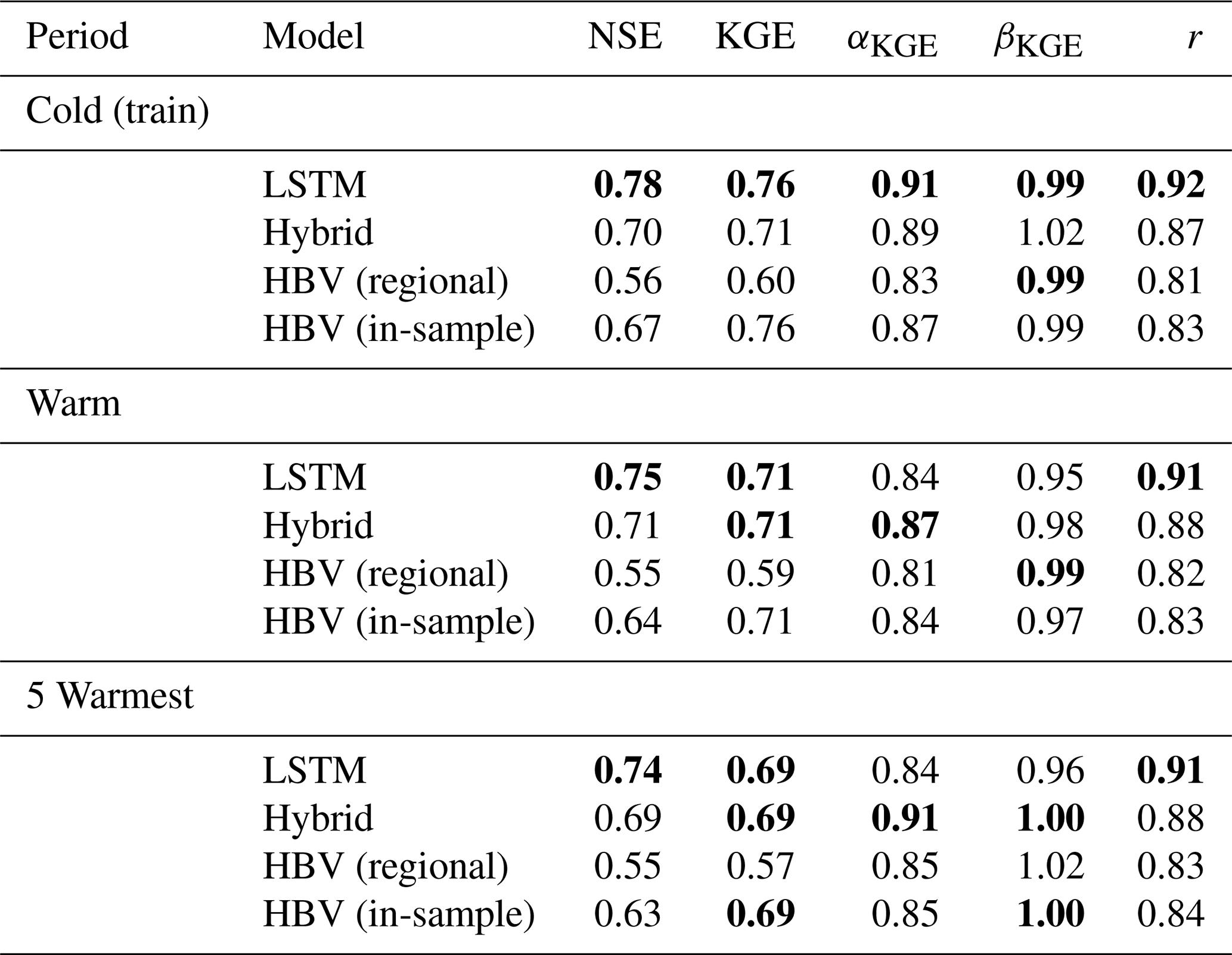
Table C4Streamflow metrics during periods with different climate conditions for the three model types: (1) data-driven (LSTM), (2) hybrid (δ-HBV), and (3) conceptual (HBV) in rainfall-dominated catchments (less than 30 % snowfall fraction). For each period and metric, the value for the best performing regional model is reported in bold text.
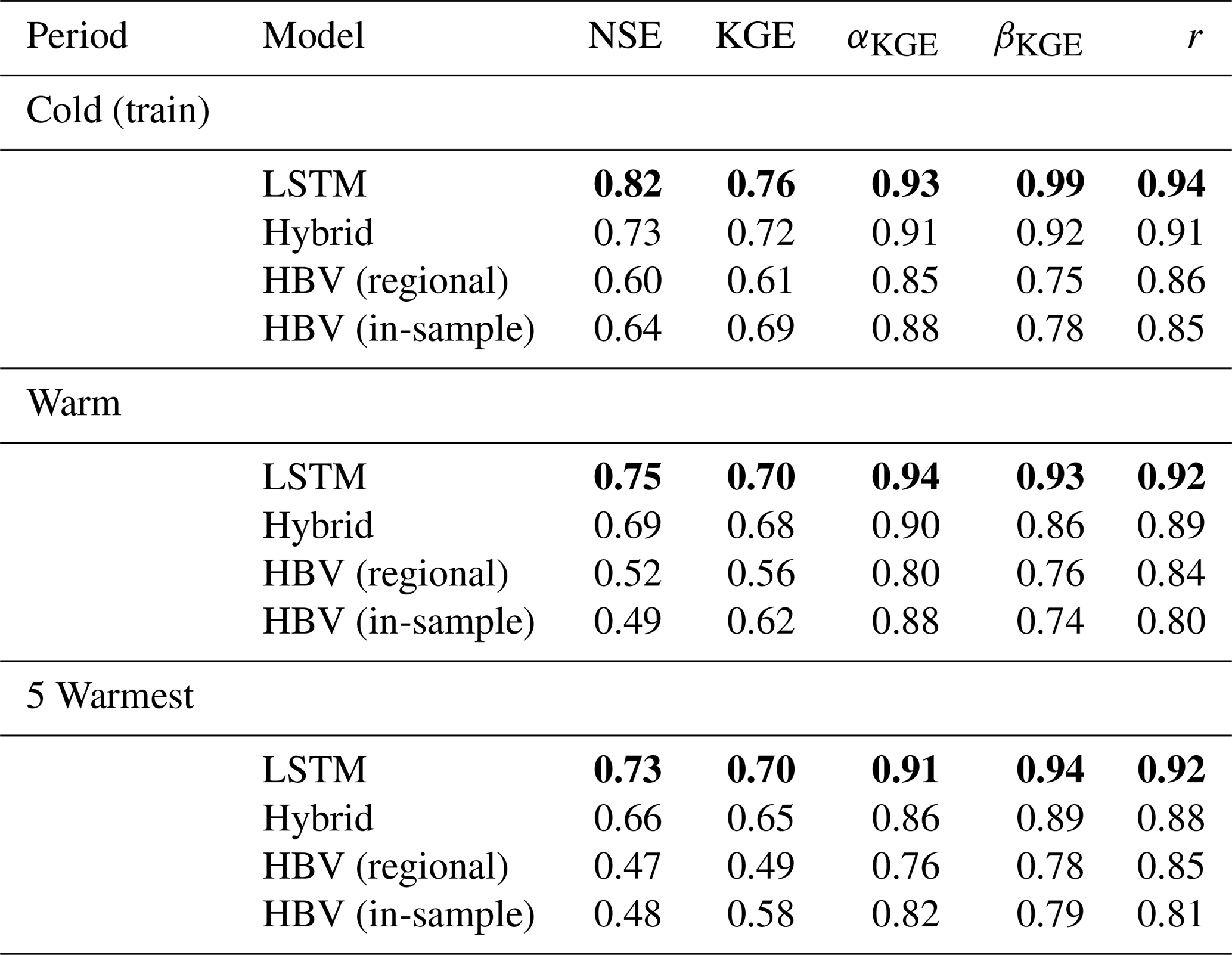
Table C5SWE metrics during periods with different climate conditions for two model types: (1) hybrid (δ-HBV), and (2) conceptual (HBV) in snow-dominated catchments (more than 30 % snowfall fraction) with little glacier influence (less than 2 % glacier cover). Note that the LSTM does not give direct access to simulated snowpack and was thus excluded from this analysis. For each period and metric, the value for the best performing regional model is reported in bold text.
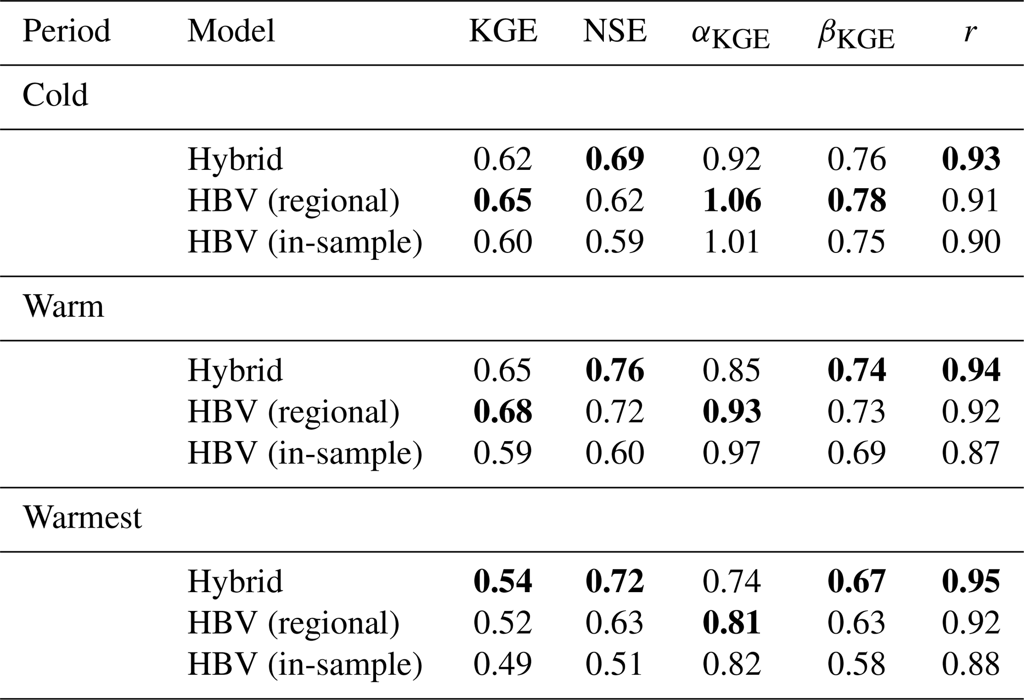
The deep learning based hydrological models were trained and evaluated using the NeuralHydrology Python library available at https://github.com/neuralhydrology/neuralhydrology (Kratzert et al., 2022). We specifically used the version provided by Acuña Espinoza et al. (2025), since it includes an implementation of the hybrid model (differentiable parameter learning (dPL) + HBV hydrologic model) developed by Feng et al. (2022a). The code that we used is available at https://doi.org/10.5281/zenodo.14191623 (Acuna Espinoza, 2024) and the original code of the hybrid model at https://doi.org/10.5281/zenodo.7943626 (Feng et al., 2022b). Small modifications were made to the code to account for our changes in the scaling of the target data for the stand-alone LSTM. To calibrate the conceptual models, we used the Python implementation of the HBV model in the Hy2DL library also provided by Acuña Espinoza et al. (2025). The code and data required to reproduce our setup are available at http://www.hydroshare.org/resource/0e708f4a9f8440c880408221d3fa86b5 (Bohl et al., 2025). The code used to compute the static catchment attributes from the HydroAtlas dataset is available through the Caravan project (https://github.com/kratzert/Caravan/tree/main/code, last access: 10 July 2026, Kratzert et al., 2023). The E-OBS meteorological data is freely available at https://doi.org/10.24381/CDS.151D3EC6 (Copernicus Climate Change Service, 2020). The SWE data for Switzerland is available at https://doi.org/10.16904/envidat.580 (Marty et al., 2025) and for Austria at https://doi.org/10.60669/fsxx-6977 (GeoSphere Austria, 2022). See Table A3, for the sources of the streamflow data, catchment shapefiles and reservoir information.
JPB, RRW, PA, CF, JP and MIB contributed to the conceptualization of the study. JPB worked on software and data curation. JPB performed the formal analyses and visualizations. JPB wrote the original draft, with all authors contributing to reviewing and editing the final draft. MIB, RRW and JP were involved in supervision.
At least one of the (co-)authors is a member of the editorial board of Hydrology and Earth System Sciences. The peer-review process was guided by an independent editor, and the authors also have no other competing interests to declare.
Publisher's note: Copernicus Publications remains neutral with regard to jurisdictional claims made in the text, published maps, institutional affiliations, or any other geographical representation in this paper. The authors bear the ultimate responsibility for providing appropriate place names. Views expressed in the text are those of the authors and do not necessarily reflect the views of the publisher.
We thank ETH Studio Davos and Academica Raetica for funding an internship of JPB at the SLF Davos.
This research has been supported by the Schweizerischer Nationalfonds zur Förderung der Wissenschaftlichen Forschung (grant no. TMSGI2_218486).
This paper was edited by Elena Toth and reviewed by two anonymous referees.
Acuna Espinoza, E.: Analyzing the generalization capabilities of hybrid hydrological models for extrapolation to extreme events, Zenodo [code], https://doi.org/10.5281/ZENODO.14191623, 2024. a
Acuña Espinoza, E., Loritz, R., Kratzert, F., Klotz, D., Gauch, M., Álvarez Chaves, M., and Ehret, U.: Analyzing the generalization capabilities of a hybrid hydrological model for extrapolation to extreme events, Hydrol. Earth Syst. Sci., 29, 1277–1294, https://doi.org/10.5194/hess-29-1277-2025, 2025. a, b, c
Andréassian, V., Bourgin, F., Oudin, L., Mathevet, T., Perrin, C., Lerat, J., Coron, L., and Berthet, L.: Seeking Genericity in the Selection of Parameter Sets: Impact on Hydrological Model Efficiency, Water Resour. Res., 50, 8356–8366, https://doi.org/10.1002/2013WR014761, 2014. a
Arsenault, R., Martel, J.-L., Brunet, F., Brissette, F., and Mai, J.: Continuous streamflow prediction in ungauged basins: long short-term memory neural networks clearly outperform traditional hydrological models, Hydrol. Earth Syst. Sci., 27, 139–157, https://doi.org/10.5194/hess-27-139-2023, 2023. a
Astagneau, P., Peters, J., Sandra, P., Muñoz-Castro, E., and Brunner, M. I.: RESIdual STability (RESIST) Calibration for Improved Hydrological Model Time Generalizability, Water Resour. Res., 62, https://doi.org/10.1029/2025WR041435, 2026. a
Bai, P., Liu, X., and Xie, J.: Simulating Runoff under Changing Climatic Conditions: A Comparison of the Long Short-Term Memory Network with Two Conceptual Hydrologic Models, J. Hydrol., 592, 125779, https://doi.org/10.1016/j.jhydrol.2020.125779, 2021. a, b
Barnett, T. P., Adam, J. C., and Lettenmaier, D. P.: Potential Impacts of a Warming Climate on Water Availability in Snow-Dominated Regions, Nature, 438, 303–309, https://doi.org/10.1038/nature04141, 2005. a
Bartholomé, E. and Belward, A. S.: GLC2000: A New Approach to Global Land Cover Mapping from Earth Observation Data, Int. J. Remote Sens., 26, 1959–1977, https://doi.org/10.1080/01431160412331291297, 2005. a, b, c, d, e, f, g
Baste, S., Klotz, D., Acuña Espinoza, E., Bardossy, A., and Loritz, R.: Unveiling the limits of deep learning models in hydrological extrapolation tasks, Hydrol. Earth Syst. Sci., 29, 5871–5891, https://doi.org/10.5194/hess-29-5871-2025, 2025. a, b
Beck, H. E., van Dijk, A. I. J. M., de Roo, A., Miralles, D. G., McVicar, T. R., Schellekens, J., and Bruijnzeel, L. A.: Global-Scale Regionalization of Hydrologic Model Parameters, Water Resour. Res., 52, 3599–3622, https://doi.org/10.1002/2015WR018247, 2016. a, b, c
Beniston, M.: Mountain Weather and Climate: A General Overview and a Focus on Climatic Change in the Alps, Hydrobiologia, 562, 3–16, https://doi.org/10.1007/s10750-005-1802-0, 2006. a
Berghuijs, W. R., Allen, S. T., Harrigan, S., and Kirchner, J. W.: Growing Spatial Scales of Synchronous River Flooding in Europe, Geophys. Res. Lett., 46, 1423–1428, https://doi.org/10.1029/2018GL081883, 2019. a, b
Berghuijs, W. R., Woods, R. A., Anderson, B. J., Hemshorn de Sánchez, A. L., and Hrachowitz, M.: Annual memory in the terrestrial water cycle, Hydrol. Earth Syst. Sci., 29, 1319–1333, https://doi.org/10.5194/hess-29-1319-2025, 2025. a
Bergström, S.: Development and Application of a Conceptual Runoff Model for Scandinavian Catchments, vol. 134, SMHI Norrköping, 1976. a, b
Bertola, M., Viglione, A., Lun, D., Hall, J., and Blöschl, G.: Flood trends in Europe: are changes in small and big floods different?, Hydrol. Earth Syst. Sci., 24, 1805–1822, https://doi.org/10.5194/hess-24-1805-2020, 2020. a, b
Beven, K.: Rainfall-Runoff Modelling: The Primer, Wiley, 1st edn., ISBN 978-0-470-71459-1 978-1-119-95100-1, https://doi.org/10.1002/9781119951001, 2012. a, b
Blöschl, G., Hall, J., Parajka, J., Perdigão, R. A. P., Merz, B., Arheimer, B., Aronica, G. T., Bilibashi, A., Bonacci, O., Borga, M., Čanjevac, I., Castellarin, A., Chirico, G. B., Claps, P., Fiala, K., Frolova, N., Gorbachova, L., Gül, A., Hannaford, J., Harrigan, S., Kireeva, M., Kiss, A., Kjeldsen, T. R., Kohnová, S., Koskela, J. J., Ledvinka, O., Macdonald, N., Mavrova-Guirguinova, M., Mediero, L., Merz, R., Molnar, P., Montanari, A., Murphy, C., Osuch, M., Ovcharuk, V., Radevski, I., Rogger, M., Salinas, J. L., Sauquet, E., Šraj, M., Szolgay, J., Viglione, A., Volpi, E., Wilson, D., Zaimi, K., and Živković, N.: Changing Climate Shifts Timing of European Floods, Science, 357, 588–590, https://doi.org/10.1126/science.aan2506, 2017. a
Bohl, J. P., Wood, R. R., Götte, J., and Brunner, M.: Generalizability of data-driven hydrological models in the European Alps, HydroShare [data set], http://www.hydroshare.org/resource/0e708f4a9f8440c880408221d3fa86b5 (last access: 10 July 2026), 2025. a
Braun, L. N. and Renner, C. B.: Application of a Conceptual Runoff Model in Different Physiographic Regions of Switzerland, Hydrol. Sci. J., 37, 217–231, https://doi.org/10.1080/02626669209492583, 1992. a
Breiman, L.: Random Forests, Mach. Learn., 45, 5–32, https://doi.org/10.1023/A:1010933404324, 2001. a
Brunner, M. I., Farinotti, D., Zekollari, H., Huss, M., and Zappa, M.: Future shifts in extreme flow regimes in Alpine regions, Hydrol. Earth Syst. Sci., 23, 4471–4489, https://doi.org/10.5194/hess-23-4471-2019, 2019. a
Brunner, M. I., Melsen, L. A., Wood, A. W., Rakovec, O., Mizukami, N., Knoben, W. J. M., and Clark, M. P.: Flood spatial coherence, triggers, and performance in hydrological simulations: large-sample evaluation of four streamflow-calibrated models, Hydrol. Earth Syst. Sci., 25, 105–119, https://doi.org/10.5194/hess-25-105-2021, 2021a. a
Brunner, M. I., Slater, L., Tallaksen, L. M., and Clark, M.: Challenges in Modeling and Predicting Floods and Droughts: A Review, WIREs Water, 8, e1520, https://doi.org/10.1002/wat2.1520, 2021b. a
Brunner, M. I., Swain, D. L., Wood, R. R., Willkofer, F., Done, J. M., Gilleland, E., and Ludwig, R.: An Extremeness Threshold Determines the Regional Response of Floods to Changes in Rainfall Extremes, Commun. Earth Environ., 2, 173, https://doi.org/10.1038/s43247-021-00248-x, 2021c. a
Brunner, M. I., Götte, J., Schlemper, C., and Van Loon, A. F.: Hydrological Drought Generation Processes and Severity Are Changing in the Alps, Geophys. Res. Lett., 50, e2022GL101776, https://doi.org/10.1029/2022GL101776, 2023. a, b
Bruno, G., Avanzi, F., Alfieri, L., Libertino, A., Gabellani, S., and Duethmann, D.: Hydrological Model Skills Change with Drought Severity; Insights from Multi-Variable Evaluation, J. Hydrol., 634, 131023, https://doi.org/10.1016/j.jhydrol.2024.131023, 2024. a, b
Carletti, F., Michel, A., Casale, F., Burri, A., Bocchiola, D., Bavay, M., and Lehning, M.: A comparison of hydrological models with different level of complexity in Alpine regions in the context of climate change, Hydrol. Earth Syst. Sci., 26, 3447–3475, https://doi.org/10.5194/hess-26-3447-2022, 2022. a
Clark, M. P., Bierkens, M. F. P., Samaniego, L., Woods, R. A., Uijlenhoet, R., Bennett, K. E., Pauwels, V. R. N., Cai, X., Wood, A. W., and Peters-Lidard, C. D.: The evolution of process-based hydrologic models: historical challenges and the collective quest for physical realism, Hydrol. Earth Syst. Sci., 21, 3427–3440, https://doi.org/10.5194/hess-21-3427-2017, 2017. a
Copernicus Climate Change Service: E-OBS Daily Gridded Meteorological Data for Europe from 1950 to Present Derived from in-Situ Observations, Copernicus Climate Change Service (C3S) Climate Data Store (CDS) [data set], https://doi.org/10.24381/CDS.151D3EC6, 2020. a, b, c, d, e, f, g, h, i, j, k, l, m
Coron, L., Andréassian, V., Perrin, C., Lerat, J., Vaze, J., Bourqui, M., and Hendrickx, F.: Crash Testing Hydrological Models in Contrasted Climate Conditions: An Experiment on 216 Australian Catchments, Water Resour. Res., 48, 2011WR011721, https://doi.org/10.1029/2011WR011721, 2012. a, b, c
Dai, A.: Increasing Drought under Global Warming in Observations and Models, Nat. Clim. Change, 3, 52–58, https://doi.org/10.1038/nclimate1633, 2013. a, b
Dakhlaoui, H., Ruelland, D., Tramblay, Y., and Bargaoui, Z.: Evaluating the Robustness of Conceptual Rainfall-Runoff Models under Climate Variability in Northern Tunisia, J. Hydrol., 550, 201–217, https://doi.org/10.1016/j.jhydrol.2017.04.032, 2017. a
DeWalle, D. R. R. A.: Modelling snowmelt runoff, 266–305 pp., Cambridge University Press, ISBN 9780521290326, https://doi.org/10.1017/cbo9780511535673.011, 2008. a
European Space Agency and Airbus: Copernicus DEM, https://doi.org/10.5270/ESA-c5d3d65, 2022. a, b
Feng, D., Lawson, K., and Shen, C.: Mitigating Prediction Error of Deep Learning Streamflow Models in Large Data-Sparse Regions With Ensemble Modeling and Soft Data, Geophys. Res. Lett., 48, e2021GL092999, https://doi.org/10.1029/2021GL092999, 2021. a
Feng, D., Liu, J., Lawson, K., and Shen, C.: Differentiable, Learnable, Regionalized Process-Based Models With Multiphysical Outputs Can Approach State-Of-The-Art Hydrologic Prediction Accuracy, Water Resour. Res., 58, e2022WR032404, https://doi.org/10.1029/2022WR032404, 2022a. a, b, c, d, e, f, g
Feng, D., Shen, C., Liu, J., Lawson, K., and Beck, H.: differentiable parameter learning (dPL) + HBV hydrologic model, Zenodo [code], https://doi.org/10.5281/ZENODO.7943626, 2022b. a
Feng, D., Beck, H., Lawson, K., and Shen, C.: The suitability of differentiable, physics-informed machine learning hydrologic models for ungauged regions and climate change impact assessment, Hydrol. Earth Syst. Sci., 27, 2357–2373, https://doi.org/10.5194/hess-27-2357-2023, 2023. a, b, c, d, e, f, g, h, i, j, k
Feng, D., Beck, H., de Bruijn, J., Sahu, R. K., Satoh, Y., Wada, Y., Liu, J., Pan, M., Lawson, K., and Shen, C.: Deep dive into hydrologic simulations at global scale: harnessing the power of deep learning and physics-informed differentiable models (δHBV-globe1.0-hydroDL), Geosci. Model Dev., 17, 7181–7198, https://doi.org/10.5194/gmd-17-7181-2024, 2024. a, b, c, d, e, f
Finger, D., Vis, M., Huss, M., and Seibert, J.: The Value of Multiple Data Set Calibration versus Model Complexity for Improving the Performance of Hydrological Models in Mountain Catchments, Water Resour. Res., 51, 1939–1958, https://doi.org/10.1002/2014WR015712, 2015. a
Fowler, K., Coxon, G., Freer, J., Peel, M., Wagener, T., Western, A., Woods, R., and Zhang, L.: Simulating Runoff Under Changing Climatic Conditions: A Framework for Model Improvement, Water Resour. Res., 54, 9812–9832, https://doi.org/10.1029/2018WR023989, 2018a. a
Fowler, K., Peel, M., Western, A., and Zhang, L.: Improved Rainfall-Runoff Calibration for Drying Climate: Choice of Objective Function, Water Resour. Res., 54, 3392–3408, https://doi.org/10.1029/2017WR022466, 2018b. a
Fowler, K. J. A., Peel, M. C., Western, A. W., Zhang, L., and Peterson, T. J.: Simulating Runoff under Changing Climatic Conditions: Revisiting an Apparent Deficiency of Conceptual Rainfall-runoff Models, Water Resour. Res., 52, 1820–1846, https://doi.org/10.1002/2015WR018068, 2016. a, b
Frame, J. M., Kratzert, F., Raney II, A., Rahman, M., Salas, F. R., and Nearing, G. S.: Post-Processing the National Water Model with Long Short-Term Memory Networks for Streamflow Predictions and Model Diagnostics, J. Am. Water Resour. As., 57, 885–905, https://doi.org/10.1111/1752-1688.12964, 2021. a, b
Frame, J. M., Kratzert, F., Klotz, D., Gauch, M., Shalev, G., Gilon, O., Qualls, L. M., Gupta, H. V., and Nearing, G. S.: Deep learning rainfall–runoff predictions of extreme events, Hydrol. Earth Syst. Sci., 26, 3377–3392, https://doi.org/10.5194/hess-26-3377-2022, 2022. a
Frame, J. M., Kratzert, F., Gupta, H. V., Ullrich, P., and Nearing, G. S.: On Strictly Enforced Mass Conservation Constraints for Modelling the Rainfall-Runoff Process, Hydrol. Process., 37, e14847, https://doi.org/10.1002/hyp.14847, 2023. a
Frei, P., Kotlarski, S., Liniger, M. A., and Schär, C.: Future snowfall in the Alps: projections based on the EURO-CORDEX regional climate models, The Cryosphere, 12, 1–24, https://doi.org/10.5194/tc-12-1-2018, 2018. a
Freudiger, D., Vis, M., and Seibert, J.: Quantifying the Contributions to Discharge of Snow and Glacier Melt. Hydro-CH2018 Project., Tech. rep., Commissioned by the Federal Office for the Environment (FOEN), Bern, Switzerland, 2020. a
Gebrechorkos, S. H., Sheffield, J., Vicente-Serrano, S. M., Funk, C., Miralles, D. G., Peng, J., Dyer, E., Talib, J., Beck, H. E., Singer, M. B., and Dadson, S. J.: Warming Accelerates Global Drought Severity, Nature, 642, 628–635, https://doi.org/10.1038/s41586-025-09047-2, 2025. a
GeoSphere Austria: SNOWGRID Klima v2.1, GeoSphere Austria [data set], https://doi.org/10.60669/FSXX-6977, 2022. a, b
Girons Lopez, M., Vis, M. J. P., Jenicek, M., Griessinger, N., and Seibert, J.: Assessing the degree of detail of temperature-based snow routines for runoff modelling in mountainous areas in central Europe, Hydrol. Earth Syst. Sci., 24, 4441–4461, https://doi.org/10.5194/hess-24-4441-2020, 2020. a, b
Goodison, B. E., Louie, P. Y. T., and Yang, D.: WMO Solid Precipitation Measurement Intercomparison, Tech. Rep. 67, WMO, Geneva, 1998. a
Götte, J., Schlemper, C., Zappa, M., and Brunner, M. I.: How Do Reservoirs Influence Streamflow Extremes? Insights from a Large-Sample Analysis in the Alpine Region, Environmental: Research Water, 1, https://doi.org/10.1088/3033-4942/ae0151, 2025. a
Gudmundsson, L., Boulange, J., Do, H. X., Gosling, S. N., Grillakis, M. G., Koutroulis, A. G., Leonard, M., Liu, J., Müller Schmied, H., Papadimitriou, L., Pokhrel, Y., Seneviratne, S. I., Satoh, Y., Thiery, W., Westra, S., Zhang, X., and Zhao, F.: Globally Observed Trends in Mean and Extreme River Flow Attributed to Climate Change, Science, 371, 1159–1162, https://doi.org/10.1126/science.aba3996, 2021. a
Guo, D., Zheng, F., Gupta, H., and Maier, H. R.: On the Robustness of Conceptual Rainfall-Runoff Models to Calibration and Evaluation Data Set Splits Selection: A Large Sample Investigation, Water Resour. Res., 56, e2019WR026752, https://doi.org/10.1029/2019WR026752, 2020. a
Gupta, H. V., Kling, H., Yilmaz, K. K., and Martinez, G. F.: Decomposition of the Mean Squared Error and NSE Performance Criteria: Implications for Improving Hydrological Modelling, J. Hydrol., 377, 80–91, https://doi.org/10.1016/j.jhydrol.2009.08.003, 2009. a, b, c, d, e
Hakala, K., Addor, N., Teutschbein, C., Vis, M., Dakhlaoui, H., and Seibert, J.: Hydrological Modeling of Climate Change Impacts, in: Encyclopedia of Water, 1–20, John Wiley & Sons, Ltd, ISBN 978-1-119-30076-2, https://doi.org/10.1002/9781119300762.wsts0062, 2019. a
Hengl, T., De Jesus, J. M., MacMillan, R. A., Batjes, N. H., Heuvelink, G. B. M., Ribeiro, E., Samuel-Rosa, A., Kempen, B., Leenaars, J. G. B., Walsh, M. G., and Gonzalez, M. R.: SoilGrids1km – Global Soil Information Based on Automated Mapping, PLoS ONE, 9, e105992, https://doi.org/10.1371/journal.pone.0105992, 2014. a, b, c, d, e, f
Hochreiter, S. and Schmidhuber, J.: Long Short-Term Memory, Neural Comput., 9, 1735–1780, https://doi.org/10.1162/neco.1997.9.8.1735, 1997. a, b
Höge, M., Scheidegger, A., Baity-Jesi, M., Albert, C., and Fenicia, F.: Improving hydrologic models for predictions and process understanding using neural ODEs, Hydrol. Earth Syst. Sci., 26, 5085–5102, https://doi.org/10.5194/hess-26-5085-2022, 2022. a, b
Hrachowitz, M., Savenije, H., Blöschl, G., McDonnell, J., Sivapalan, M., Pomeroy, J., Arheimer, B., Blume, T., Clark, M., Ehret, U., Fenicia, F., Freer, J., Gelfan, A., Gupta, H., Hughes, D., Hut, R., Montanari, A., Pande, S., Tetzlaff, D., Troch, P., Uhlenbrook, S., Wagener, T., Winsemius, H., Woods, R., Zehe, E., and Cudennec, C.: A Decade of Predictions in Ungauged Basins (PUB) – a Review, Hydrol. Sci. J., 58, 1198–1255, https://doi.org/10.1080/02626667.2013.803183, 2013. a, b
Janzing, J., Wanders, N., van Tiel, M., van Jaarsveld, B., Karger, D. N., and Brunner, M. I.: Hyper-resolution large-scale hydrological modelling benefits from improved process representation in mountain regions, Hydrol. Earth Syst. Sci., 29, 7041–7071, https://doi.org/10.5194/hess-29-7041-2025, 2025. a
Ji, H. K., Mirzaei, M., Lai, S. H., Dehghani, A., and Dehghani, A.: The Robustness of Conceptual Rainfall-Runoff Modelling under Climate Variability – A Review, J. Hydrol., 621, 129666, https://doi.org/10.1016/j.jhydrol.2023.129666, 2023. a
Karpatne, A., Atluri, G., Faghmous, J. H., Steinbach, M., Banerjee, A., Ganguly, A., Shekhar, S., Samatova, N., and Kumar, V.: Theory-Guided Data Science: A New Paradigm for Scientific Discovery from Data, IEEE T. Knowl. Data Eng., 29, 2318–2331, https://doi.org/10.1109/TKDE.2017.2720168, 2017. a
Keller, A. A., Garner, K., Rao, N., Knipping, E., and Thomas, J.: Hydrological Models for Climate-Based Assessments at the Watershed Scale: A Critical Review of Existing Hydrologic and Water Quality Models, Sci. Total Environ., 867, 161209, https://doi.org/10.1016/j.scitotenv.2022.161209, 2023. a
Kingma, D. P. and Ba, J.: Adam: A Method for Stochastic Optimization, arXiv [preprint], https://doi.org/10.48550/arXiv.1412.6980, 2017. a
Klemeš, V.: Operational Testing of Hydrological Simulation Models, Hydrol. Sci. J., 31, 13–24, https://doi.org/10.1080/02626668609491024, 1986. a, b
Klingler, C., Schulz, K., and Herrnegger, M.: LamaH-CE: LArge-SaMple DAta for Hydrology and Environmental Sciences for Central Europe, Earth Syst. Sci. Data, 13, 4529–4565, https://doi.org/10.5194/essd-13-4529-2021, 2021. a
Klotz, D., Miersch, P., do Nascimento, T. V. M., Fenicia, F., Gauch, M., and Zscheischler, J.: EARLS: A runoff reconstruction dataset for Europe, Earth Syst. Sci. Data Discuss. [preprint], https://doi.org/10.5194/essd-2024-450, in review, 2025. a
Koh, P. W., Sagawa, S., Marklund, H., Xie, S. M., Zhang, M., Balsubramani, A., Hu, W., Yasunaga, M., Phillips, R. L., Gao, I., Lee, T., David, E., Stavness, I., Guo, W., Earnshaw, B., Haque, I., Beery, S. M., Leskovec, J., Kundaje, A., Pierson, E., Levine, S., Finn, C., and Liang, P.: WILDS: A Benchmark of in-the-Wild Distribution Shifts, in: Proceedings of the 38th International Conference on Machine Learning, edited by: Meila, M. and Zhang, T., vol. 139 of Proceedings of Machine Learning Research, pp. 5637–5664, PMLR, 2021. a
Kraft, B., Jung, M., Körner, M., Koirala, S., and Reichstein, M.: Towards hybrid modeling of the global hydrological cycle, Hydrol. Earth Syst. Sci., 26, 1579–1614, https://doi.org/10.5194/hess-26-1579-2022, 2022. a, b
Kraft, B., Schirmer, M., Aeberhard, W. H., Zappa, M., Seneviratne, S. I., and Gudmundsson, L.: CH-RUN: a deep-learning-based spatially contiguous runoff reconstruction for Switzerland, Hydrol. Earth Syst. Sci., 29, 1061–1082, https://doi.org/10.5194/hess-29-1061-2025, 2025. a, b
Kratzert, F., Klotz, D., Brenner, C., Schulz, K., and Herrnegger, M.: Rainfall–runoff modelling using Long Short-Term Memory (LSTM) networks, Hydrol. Earth Syst. Sci., 22, 6005–6022, https://doi.org/10.5194/hess-22-6005-2018, 2018. a, b
Kratzert, F., Klotz, D., Herrnegger, M., Sampson, A. K., Hochreiter, S., and Nearing, G. S.: Toward Improved Predictions in Ungauged Basins: Exploiting the Power of Machine Learning, Water Resour. Res., 55, 11344–11354, https://doi.org/10.1029/2019WR026065, 2019a. a, b
Kratzert, F., Klotz, D., Shalev, G., Klambauer, G., Hochreiter, S., and Nearing, G.: Towards learning universal, regional, and local hydrological behaviors via machine learning applied to large-sample datasets, Hydrol. Earth Syst. Sci., 23, 5089–5110, https://doi.org/10.5194/hess-23-5089-2019, 2019b. a, b, c, d, e, f, g, h
Kratzert, F., Gauch, M., Nearing, G., and Klotz, D.: NeuralHydrology — A Python Library for Deep Learningresearch in Hydrology, J. Open Source Softw., 7, 4050, https://doi.org/10.21105/joss.04050, 2022. a, b
Kratzert, F., Nearing, G., Addor, N., Erickson, T., Gauch, M., Gilon, O., Gudmundsson, L., Hassidim, A., Klotz, D., Nevo, S., Shalev, G., and Matias, Y.: Caravan – A Global Community Dataset for Large-Sample Hydrology, Sci. Data, 10, 61, https://doi.org/10.1038/s41597-023-01975-w, 2023. a, b
Kratzert, F., Gauch, M., Klotz, D., and Nearing, G.: HESS Opinions: Never train a Long Short-Term Memory (LSTM) network on a single basin, Hydrol. Earth Syst. Sci., 28, 4187–4201, https://doi.org/10.5194/hess-28-4187-2024, 2024. a
Krueger, D., Caballero, E., Jacobsen, J.-H., Zhang, A., Binas, J., Zhang, D., Priol, R. L., and Courville, A.: Out-of-Distribution Generalization via Risk Extrapolation (REx), in: Proceedings of the 38th International Conference on Machine Learning, 5815–5826, PMLR, ISSN 2640-3498, 2021. a
Kuhn, D., Shafiee, S., and Wiesemann, W.: Distributionally Robust Optimization, arXiv [preprint], https://doi.org/10.48550/arXiv.2411.02549, 2024. a
Comité Français des Barrages et Réservoirs: Monographies Barrages, http://www.barrages-cfbr.eu/ (last access: 10 July 2026), 2022. a
LeCun, Y. A., Bottou, L., Orr, G. B., and Müller, K.-R.: Efficient BackProp, in: Neural Networks: Tricks of the Trade: Second Edition, edited by: Montavon, G., Orr, G. B., and Müller, K.-R., 9–48, Springer, Berlin, Heidelberg, ISBN 978-3-642-35289-8, https://doi.org/10.1007/978-3-642-35289-8_3, 2012. a
Lehner, B., Messager, M. L., Korver, M. C., and Linke, S.: Global Hydro-Environmental Lake Characteristics at High Spatial Resolution, Sci. Data, 9, 351, https://doi.org/10.1038/s41597-022-01425-z, 2022. a
Lemaitre-Basset, T., Collet, L., Thirel, G., Parajka, J., Evin, G., and Hingray, B.: Climate Change Impact and Uncertainty Analysis on Hydrological Extremes in a French Mediterranean Catchment, Hydrol. Sci. J., 66, 888–903, https://doi.org/10.1080/02626667.2021.1895437, 2021. a
Lindström, G., Johansson, B., Persson, M., Gardelin, M., and Bergström, S.: Development and Test of the Distributed HBV-96 Hydrological Model, J. Hydrol., 201, 272–288, https://doi.org/10.1016/S0022-1694(97)00041-3, 1997. a, b
Linke, S., Lehner, B., Ouellet Dallaire, C., Ariwi, J., Grill, G., Anand, M., Beames, P., Burchard-Levine, V., Maxwell, S., Moidu, H., Tan, F., and Thieme, M.: Global Hydro-Environmental Sub-Basin and River Reach Characteristics at High Spatial Resolution, Sci. Data, 6, 283, https://doi.org/10.1038/s41597-019-0300-6, 2019. a
Liu, J., Hu, Z., Cui, P., Li, B., and Shen, Z.: Heterogeneous Risk Minimization, arXiv [preprint], https://doi.org/10.48550/arXiv.2105.03818, 2021. a
Liu, J., Shen, Z., He, Y., Zhang, X., Xu, R., Yu, H., and Cui, P.: Towards Out-Of-Distribution Generalization: A Survey, arXiv [preprint], https://doi.org/10.48550/arXiv.2108.13624, 2023. a
Liu, J., Koch, J., Stisen, S., Troldborg, L., and Schneider, R. J. M.: A national-scale hybrid model for enhanced streamflow estimation – consolidating a physically based hydrological model with long short-term memory (LSTM) networks, Hydrol. Earth Syst. Sci., 28, 2871–2893, https://doi.org/10.5194/hess-28-2871-2024, 2024. a
Madsen, H., Lawrence, D., Lang, M., Martinkova, M., and Kjeldsen, T. R.: Review of Trend Analysis and Climate Change Projections of Extreme Precipitation and Floods in Europe, J. Hydrol., 519, 3634–3650, https://doi.org/10.1016/j.jhydrol.2014.11.003, 2014. a
Mai, J., Shen, H., Tolson, B. A., Gaborit, É., Arsenault, R., Craig, J. R., Fortin, V., Fry, L. M., Gauch, M., Klotz, D., Kratzert, F., O'Brien, N., Princz, D. G., Rasiya Koya, S., Roy, T., Seglenieks, F., Shrestha, N. K., Temgoua, A. G. T., Vionnet, V., and Waddell, J. W.: The Great Lakes Runoff Intercomparison Project Phase 4: the Great Lakes (GRIP-GL), Hydrol. Earth Syst. Sci., 26, 3537–3572, https://doi.org/10.5194/hess-26-3537-2022, 2022. a
Martel, J.-L., Brissette, F., Arsenault, R., Turcotte, R., Castañeda-Gonzalez, M., Armstrong, W., Mailhot, E., Pelletier-Dumont, J., Rondeau-Genesse, G., and Caron, L.-P.: Assessing the adequacy of traditional hydrological models for climate change impact studies: a case for long short-term memory (LSTM) neural networks, Hydrol. Earth Syst. Sci., 29, 2811–2836, https://doi.org/10.5194/hess-29-2811-2025, 2025. a, b, c
Marty, C., Michel, A., and Jonas, T.: SPASS – New Gridded Climatological Snow Datasets for Switzerland, EnviDat [data set], https://doi.org/10.16904/envidat.580, 2025. a, b
Mendenhall, W., Wackerly, D. D., and Scheaffer, R. L.: Mathematical Statistics with Applications, International Student Edition, PWS-Kent Publ. Co., Boston, 4th edn., ISBN 0-534-98166-6, 1990. a
Meyer, J., Kohn, I., Stahl, K., Hakala, K., Seibert, J., and Cannon, A. J.: Effects of univariate and multivariate bias correction on hydrological impact projections in alpine catchments, Hydrol. Earth Syst. Sci., 23, 1339–1354, https://doi.org/10.5194/hess-23-1339-2019, 2019. a
Michel, A., Aschauer, J., Jonas, T., Gubler, S., Kotlarski, S., and Marty, C.: SnowQM 1.0: a fast R package for bias-correcting spatial fields of snow water equivalent using quantile mapping, Geosci. Model Dev., 17, 8969–8988, https://doi.org/10.5194/gmd-17-8969-2024, 2024. a
Mizukami, N., Rakovec, O., Newman, A. J., Clark, M. P., Wood, A. W., Gupta, H. V., and Kumar, R.: On the choice of calibration metrics for “high-flow” estimation using hydrologic models, Hydrol. Earth Syst. Sci., 23, 2601–2614, https://doi.org/10.5194/hess-23-2601-2019, 2019. a
Mountain Research Initiative EDW Working Group: Elevation-Dependent Warming in Mountain Regions of the World, Nat. Clim. Change, 5, 424–430, https://doi.org/10.1038/nclimate2563, 2015. a
Muelchi, R., Rössler, O., Schwanbeck, J., Weingartner, R., and Martius, O.: An Ensemble of Daily Simulated Runoff Data (1981–2099) under Climate Change Conditions for 93 Catchments in Switzerland (Hydro-CH2018-Runoff Ensemble), Geosci. Data J., 9, 46–57, https://doi.org/10.1002/gdj3.117, 2022. a
Muñoz-Castro, E., Anderson, B. J., Astagneau, P. C., Swain, D. L., Mendoza, P. A., and Brunner, M. I.: How well do hydrological models simulate streamflow extremes and drought-to-flood transitions?, Hydrol. Earth Syst. Sci., 30, 825–848, https://doi.org/10.5194/hess-30-825-2026, 2026. a
Nash, J. and Sutcliffe, J.: River Flow Forecasting through Conceptual Models Part I — A Discussion of Principles, J. Hydrol., 10, 282–290, https://doi.org/10.1016/0022-1694(70)90255-6, 1970. a, b
Nicolle, P., Andréassian, V., Royer-Gaspard, P., Perrin, C., Thirel, G., Coron, L., and Santos, L.: Technical note: RAT – a robustness assessment test for calibrated and uncalibrated hydrological models, Hydrol. Earth Syst. Sci., 25, 5013–5027, https://doi.org/10.5194/hess-25-5013-2021, 2021. a
Olefs, M., Koch, R., Schöner, W., and Marke, T.: Changes in Snow Depth, Snow Cover Duration, and Potential Snowmaking Conditions in Austria, 1961–2020 – A Model Based Approach, Atmosphere, 11, 1330, https://doi.org/10.3390/atmos11121330, 2020. a
Oudin, L., Andréassian, V., Perrin, C., Michel, C., and Le Moine, N.: Spatial Proximity, Physical Similarity, Regression and Ungaged Catchments: A Comparison of Regionalization Approaches Based on 913 French Catchments, Water Resour. Res., 44, https://doi.org/10.1029/2007WR006240, 2008. a
Páez Mendieta, J. D., Geriberto Hidalgo, I., and Cioffi, F.: Impact of Different Hydrological Models on Hydroelectric Operation Planning, Renewable Energy, 232, 120975, https://doi.org/10.1016/j.renene.2024.120975, 2024. a
Partl, R.: Statistik 1977 Der Großen Talsperren Und Flußstauwerke Österreichs, Tech. rep., Eigenverl. d. Österreich. Wasserwirtschaftsverbandes., 1977. a, b
Peters, J., Bühlmann, P., and Meinshausen, N.: Causal Inference by Using Invariant Prediction: Identification and Confidence Intervals, J. Roy. Stat. Soc. B, 78, 947–1012, https://doi.org/10.1111/rssb.12167, 2016. a
Reichert, P., Ma, K., Höge, M., Fenicia, F., Baity-Jesi, M., Feng, D., and Shen, C.: Metamorphic testing of machine learning and conceptual hydrologic models, Hydrol. Earth Syst. Sci., 28, 2505–2529, https://doi.org/10.5194/hess-28-2505-2024, 2024. a, b, c, d, e, f, g
Rentschler, J., Salhab, M., and Jafino, B. A.: Flood Exposure and Poverty in 188 Countries, Nat. Commun., 13, 3527, https://doi.org/10.1038/s41467-022-30727-4, 2022. a
RGI Consortium: Randolph Glacier Inventory – a Dataset of Global Glacier Outlines, Version 2, Boulder, Colorado USA, National Snow and Ice Data Center [data set], https://doi.org/10.7265/cc6e-zp12, 2012. a, b
Robinson, N., Regetz, J., and Guralnick, R. P.: EarthEnv-DEM90: A Nearly-Global, Void-Free, Multi-Scale Smoothed, 90m Digital Elevation Model from Fused ASTER and SRTM Data, ISPRS J. Photogramm. Remote, 87, 57–67, https://doi.org/10.1016/j.isprsjprs.2013.11.002, 2014. a, b, c, d, e, f
Rumelhart, D. E., Hinton, G. E. and Williams, R. J.: Learning Internal Representations by Error Propagation, in: Parallel Distributed Processing: Explorations in the Microstructure of Cognition: Foundations, edited by: Rumelhart, D. E. and McClelland, J. L., 318–362, MIT Press, ISBN 9780262291408, https://doi.org/10.7551/mitpress/5236.001.0001, 1987. a
Santos, L., Andréassian, V., Sonnenborg, T. O., Lindström, G., de Lavenne, A., Perrin, C., Collet, L., and Thirel, G.: Lack of robustness of hydrological models: a large-sample diagnosis and an attempt to identify hydrological and climatic drivers, Hydrol. Earth Syst. Sci., 29, 683–700, https://doi.org/10.5194/hess-29-683-2025, 2025. a, b
Sauquet, E., Beaufort, A., Sarremejane, R., and Thirel, G.: Predicting Flow Intermittence in France under Climate Change, Hydrol. Sci. J., 66, 2046–2059, https://doi.org/10.1080/02626667.2021.1963444, 2021. a
Schwarb, M.: The Alpine Precipitation Climate: Evaluation of a High-Resolution Analysis Scheme Using Comprehensive Rain-Gauge Data, Ph.D. thesis, ETH Zurich, https://doi.org/10.3929/ETHZ-A-004121274, 2000. a
Schwarzwald, K. and Geil, K.: Xagg: A Python Package to Aggregate Gridded Data onto Polygons, J. Open Source Softw., 9, 7239, https://doi.org/10.21105/joss.07239, 2024. a
Seibert, J.: Reliability of Model Predictions Outside Calibration Conditions, Hydrol. Res., 34, 477–492, https://doi.org/10.2166/nh.2003.0019, 2003. a, b
Seibert, J. and Bergström, S.: A retrospective on hydrological catchment modelling based on half a century with the HBV model, Hydrol. Earth Syst. Sci., 26, 1371–1388, https://doi.org/10.5194/hess-26-1371-2022, 2022. a
Seibert, J. and Vis, M. J. P.: Teaching hydrological modeling with a user-friendly catchment-runoff-model software package, Hydrol. Earth Syst. Sci., 16, 3315–3325, https://doi.org/10.5194/hess-16-3315-2012, 2012. a, b
Shen, C., Appling, A. P., Gentine, P., Bandai, T., Gupta, H., Tartakovsky, A., Baity-Jesi, M., Fenicia, F., Kifer, D., Li, L., Liu, X., Ren, W., Zheng, Y., Harman, C. J., Clark, M., Farthing, M., Feng, D., Kumar, P., Aboelyazeed, D., Rahmani, F., Song, Y., Beck, H. E., Bindas, T., Dwivedi, D., Fang, K., Höge, M., Rackauckas, C., Mohanty, B., Roy, T., Xu, C., and Lawson, K.: Differentiable Modelling to Unify Machine Learning and Physical Models for Geosciences, Nat. Rev. Earth Environ., 4, 552–567, https://doi.org/10.1038/s43017-023-00450-9, 2023. a
Simmler, H.: Die Talsperren Österreichs : Statistik 1961., Die Talsperren Österreichs, Schriftenreihe ; 12, Springer Vienna / Österreichische Staubeckenkommision, Vienna, 1st edn., ISBN 3-7091-5546-0, 1962. a, b
Slater, L. J., Arnal, L., Boucher, M.-A., Chang, A. Y.-Y., Moulds, S., Murphy, C., Nearing, G., Shalev, G., Shen, C., Speight, L., Villarini, G., Wilby, R. L., Wood, A., and Zappa, M.: Hybrid forecasting: blending climate predictions with AI models, Hydrol. Earth Syst. Sci., 27, 1865–1889, https://doi.org/10.5194/hess-27-1865-2023, 2023. a
Speckhann, G. A., Kreibich, H., and Merz, B.: Inventory of dams in Germany, Earth Syst. Sci. Data, 13, 731–740, https://doi.org/10.5194/essd-13-731-2021, 2021. a, b, c
Thirel, G., Santos, L., Delaigue, O., and Perrin, C.: On the use of streamflow transformations for hydrological model calibration, Hydrol. Earth Syst. Sci., 28, 4837–4860, https://doi.org/10.5194/hess-28-4837-2024, 2024. a, b
Tolson, B. A. and Shoemaker, C. A.: Dynamically Dimensioned Search Algorithm for Computationally Efficient Watershed Model Calibration, Water Resour. Res., 43, 2005WR004723, https://doi.org/10.1029/2005WR004723, 2007. a
Tsai, W.-P., Feng, D., Pan, M., Beck, H., Lawson, K., Yang, Y., Liu, J., and Shen, C.: From Calibration to Parameter Learning: Harnessing the Scaling Effects of Big Data in Geoscientific Modeling, Nat. Commun., 12, 5988, https://doi.org/10.1038/s41467-021-26107-z, 2021. a
United Nations Office for Disaster Risk Reduction (UNDRR) and Centre for Research on the Epidemiology of Disasters (CRED): The Human Cost of Disasters: An Overview of the Last 20 Years (2000–2019), Tech. rep., United Nations Office for Disaster Reduction, and Centre for Research on the Epidemiology of Disasters, https://www.undrr.org/publication/human-cost-disasters-overview-last-20-years-2000-2019 (last access: 10 July 2026), 2020. a
Uzun, S., Tanir, T., Coelho, G. d. A., de Souza de Lima, A., Cassalho, F., and Ferreira, C. M.: Changes in Snowmelt Runoff Timing in the Contiguous United States, Hydrol. Process., 35, e14430, https://doi.org/10.1002/hyp.14430, 2021. a
Van Der Wiel, K., Wanders, N., Selten, F. M., and Bierkens, M. F. P.: Added Value of Large Ensemble Simulations for Assessing Extreme River Discharge in a 2 ∘C Warmer World, Geophys. Res. Lett., 46, 2093–2102, https://doi.org/10.1029/2019GL081967, 2019. a
Vasudevan, R. K., Ziatdinov, M., Vlcek, L., and Kalinin, S. V.: Off-the-Shelf Deep Learning Is Not Enough, and Requires Parsimony, Bayesianity, and Causality, npj Computational Materials, 7, 16, https://doi.org/10.1038/s41524-020-00487-0, 2021. a
Vaze, J., Post, D., Chiew, F., Perraud, J.-M., Viney, N., and Teng, J.: Climate Non-Stationarity – Validity of Calibrated Rainfall–Runoff Models for Use in Climate Change Studies, J. Hydrol., 394, 447–457, https://doi.org/10.1016/j.jhydrol.2010.09.018, 2010. a, b
Wagener, T., McIntyre, N., Lees, M. J., Wheater, H. S., and Gupta, H. V.: Towards Reduced Uncertainty in Conceptual Rainfall-runoff Modelling: Dynamic Identifiability Analysis, Hydrol. Process., 17, 455–476, https://doi.org/10.1002/hyp.1135, 2003. a
Wang, J., Lan, C., Liu, C., Ouyang, Y., Qin, T., Lu, W., Chen, Y., Zeng, W., and Yu, P.: Generalizing to Unseen Domains: A Survey on Domain Generalization, IEEE T. Knowl. Data Eng., 35, 8052–8072, https://doi.org/10.1109/TKDE.2022.3178128, 2022. a
Warscher, M., Strasser, U., Kraller, G., Marke, T., Franz, H., and Kunstmann, H.: Performance of Complex Snow Cover Descriptions in a Distributed Hydrological Model System: A Case Study for the High Alpine Terrain of the Berchtesgaden Alps, Water Resour. Res., 49, 2619–2637, https://doi.org/10.1002/wrcr.20219, 2013. a
Wi, S. and Steinschneider, S.: Assessing the Physical Realism of Deep Learning Hydrologic Model Projections Under Climate Change, Water Resour. Res., 58, e2022WR032123, https://doi.org/10.1029/2022WR032123, 2022. a, b, c, d, e, f, g
Wi, S. and Steinschneider, S.: On the need for physical constraints in deep learning rainfall–runoff projections under climate change: a sensitivity analysis to warming and shifts in potential evapotranspiration, Hydrol. Earth Syst. Sci., 28, 479–503, https://doi.org/10.5194/hess-28-479-2024, 2024. a, b, c, d, e, f, g, h
Williams, P. and Ford, D. C.: Global Distribution of Carbonate Rocks, Schweizerbart Science Publishers, ISBN 9783443211479, 2006. a
Willkofer, F., Wood, R. R., von Trentini, F., Weismüller, J., Poschlod, B., and Ludwig, R.: A Holistic Modelling Approach for the Estimation of Return Levels of Peak Flows in Bavaria, Water, 12, 2349, https://doi.org/10.3390/w12092349, 2020. a
Willkofer, F., Wood, R. R., and Ludwig, R.: Assessing the impact of climate change on high return levels of peak flows in Bavaria applying the CRCM5 large ensemble, Hydrol. Earth Syst. Sci., 28, 2969–2989, https://doi.org/10.5194/hess-28-2969-2024, 2024. a, b
Xing, Z., Ma, M., Su, Z., Lv, J., Yi, P., and Song, W.: A review of the adaptability of hydrological models for drought forecasting, Proc. IAHS, 383, 261–266, https://doi.org/10.5194/piahs-383-261-2020, 2020. a
- Abstract
- Introduction
- Data and Methods
- Results
- Discussion
- Conclusions
- Appendix A: Data
- Appendix B: Model details
- Appendix C: Model accuracy and generalizability
- Code and data availability
- Author contributions
- Competing interests
- Disclaimer
- Acknowledgements
- Financial support
- Review statement
- References
- Abstract
- Introduction
- Data and Methods
- Results
- Discussion
- Conclusions
- Appendix A: Data
- Appendix B: Model details
- Appendix C: Model accuracy and generalizability
- Code and data availability
- Author contributions
- Competing interests
- Disclaimer
- Acknowledgements
- Financial support
- Review statement
- References