Comparing multi-model mosaic and multi-model combination methods to simulate streamflow across the contiguous USA

The ability to accurately predict streamflow underpins decisions in water management, flood prevention, and sectoral planning. Traditional approaches for streamflow prediction often rely on a single model, thereby overlooking potential benefits from using multiple models. To address this limitation, this study explores alternative methods that select and combine multiple models to enhance streamflow simulations. Specifically, we assess the performance of multi-model mosaic methods that assign a single model to each catchment, and multi-model combination methods that merge multiple models using static or dynamic weighting schemes. The Framework for Understanding Structural Errors (FUSE) is used to create an ensemble of 78 hydrological models, which were applied to 544 catchments from the CAMELS dataset across the contiguous United States. Each of the 78 models is calibrated utilizing a composite objective function, calculated as the average of a high-flow and a low-flow performance metric, to cover a wide range of streamflow conditions. Based on our selection of lumped FUSE models, the results show that a carefully chosen single model from a larger ensemble can closely approach the performance of more complex multi-model strategies. Among the multi-model approaches, the combination and mosaic methods show broadly similar overall skill, although the combination approaches deliver slightly higher performance and lower sampling uncertainty. However, per-catchment differences persist, indicating that no single multi-model strategy dominates everywhere. This heterogeneity in performance makes it difficult to determine a priori which multi-model method will best represent streamflow in a given catchment.

1 Introduction

In hydrology, applications such as water resource management, climate impact assessment, and flood prediction usually rely on hydrologic modelling. Yet, this task remains difficult given the complexity of most catchments, where numerous hydrologic processes are intertwined. Consequently, representing these interactions within a single modelling framework that covers large spatial domains remains a central challenge. Over the years, numerous hydrological models have emerged, most of which were developed to meet a specific need in a specific area (Singh and Woolhiser, 2002; Clark et al., 2011; Sidle, 2021; Horton et al., 2022). The substantial differences among hydrological models in their data requirements, process representations, and parameterizations make it unlikely that any single model will outperform all others across all catchments; in other words, identifying a “one-size-fits-all” model is difficult (Andréassian et al., 2009; Savenije, 2009). Nevertheless, despite these challenges, the ambition of developing broadly applicable hydrological models has long been present in the discipline (e.g., Perrin et al., 2003; Beck et al., 2016; Arheimer et al., 2020; Mathevet et al., 2020). Linsley (1982) already argued that general modelling frameworks would make it unnecessary for each hydrologist to develop his or her own model for each catchment, highlighting that repeated application of the same model enhances cumulative learning.

Moreover, there are often only weak relationships between model performance and catchment geological, topographical, soil, and vegetation characteristics (Addor et al., 2018; Knoben et al., 2020; David et al., 2022). Hence, it remains challenging to determine which model is most appropriate for a given modelling project. The difficulty – and the potential lack of hydrologic realism – of selecting a single model for individual catchments or across multiple catchments has motivated the use of multi-model approaches, where the choice of models may vary across space (Georgakakos et al., 2004; Knoben et al., 2020; Wan et al., 2021; Thébault et al., 2024; Spieler and Schütze, 2024).

While traditional hydrologic modelling often relies on a single model structure, multi-model approaches are increasingly explored for their potential to enhance predictive reliability and inform decision-making (Refsgaard et al., 2007; Ramos et al., 2013; Dion et al., 2021; Ogden et al., 2021; Caillouet et al., 2022; Johnson et al., 2023). Multi-model approaches can be implemented either as ensembles, which retain multiple simulations to characterize uncertainty, or as deterministic selections/combinations that aim to produce a single best estimate. Although we acknowledge the benefits of ensemble multi-model methods – namely, their ability to explicitly characterize structural uncertainty and provide probabilistic predictions (e.g., Thébault et al., 2025b) – the use of ensemble model configurations is outside the scope of our study.

Here, we focus instead on two complementary multi-model paradigms: (1) multi-model mosaics, and (2) multi-model combinations. For a given selection of catchments, multi-model mosaics aim to assign a single suitable model from a larger ensemble of available models to each catchment. Note that this term has been increasingly used in recent hydrological literature to describe spatial model selection approaches across large domains (e.g., Ogden et al., 2021; Johnson et al., 2023; Knoben et al., 2025; Thébault et al., 2025b; Ogden et al., 2026). For such an approach, the main question to answer is: how should this model selection be made? In contrast, multi-model combinations aim to take advantage of the potential complementarity of hydrological models within a given catchment and seek to create suitable multi-model combinations for each catchment. The question to answer here is: how can multiple models be effectively combined? There is currently limited guidance on the implementation of multi-model mosaic and multi-model combination methods.

For multi-model mosaics, one possible implementation strategy is to select models in specific catchments based on aggregate measures of model performance (e.g., the Nash-Sutcliffe or Kling-Gupta efficiency metrics). Early large-sample model intercomparison studies already demonstrated that no single model structure consistently outperforms others across all catchments (e.g., Perrin et al., 2001). Subsequent applications explored spatial model selection strategies (e.g., van Esse et al., 2013), illustrating both the potential and the challenges associated with mosaic-type approaches. Performance-based selection generally leads to higher overall performance across large domains compared to a one-size-fits-all model approach (Knoben et al., 2020; Mai et al., 2022; Thébault et al., 2024). However, this approach introduces several challenges. First, as highlighted by multiple authors (Perrin et al., 2001; Thébault et al., 2024; Knoben et al., 2025), the multi-model mosaic based on performance exhibits a highly heterogeneous pattern, with many different models identified as locally optimal across the domain. Second, many previous studies have demonstrated that there is a high degree of equifinality between models (Beven, 2006) – while a single model may perform slightly better than others for a specific catchment, the performance difference between the best and the next-best models is often very small (Knoben et al., 2020; Spieler and Schütze, 2024; Knoben et al., 2025). This non-uniqueness of models highlights the uncertainty surrounding the choice of specific model structures and is compounded by the fact that the performance scores used for model selection can themselves be highly uncertain and overly sensitive to model errors on individual time steps (see e.g. Brigode et al., 2015; Newman et al., 2015; Clark et al., 2021; Klotz et al., 2024). The dual problems of lack of spatial coherence and non-uniqueness of models make it difficult to reliably identify a single best model for any given catchment or to link model performance to the physical characteristics of the catchments. An alternative selection strategy is landscape-based, where models are chosen to match dominant processes. Although this approach can be promising, it typically requires substantial expert judgement and detailed catchment information that are rarely available consistently at large scales (McMillan et al., 2023) and is therefore not considered further here.

For multi-model combinations, the most common approach is based on weighted average multi-model combination algorithms such as Bayesian Model Averaging (Raftery et al., 2005; Vrugt et al., 2008). These methods have shown improvements in performance compared with one-size-fits-all models over large domains (Shamseldin et al., 1997; Georgakakos et al., 2004; Seiller et al., 2012; Thébault et al., 2024). However, assigning weights to the different members of the hydrological ensemble is not trivial and is still widely debated in the scientific community. For example, Arsenault et al. (2015), Wan et al. (2021), and Todorović et al. (2024) compare different algorithms for streamflow combinations and highlight that it is difficult to establish the benefits of one method over another. Furthermore, combination methods also suffer from issues of spatial coherence and model equifinality over large domains, which limits their ability to consistently represent regional hydrologic behaviour or to provide physically interpretable relationships between model performance and catchment characteristics.

Despite these challenges, some general principles for building an effective multi-model ensemble can be found in the literature. Winter and Nychka (2010) showed that the key to multi-model approaches does not lie in the number of models but in their differences: the effectiveness of an ensemble increases when one model's strengths can compensate for another's weaknesses. Seiller et al. (2012) highlighted that an individually “poor” (low-performing) model may occasionally provide useful information to the ensemble. Several studies have emphasised the importance of accounting for model diversity, fidelity, and sensitivity when constructing ensembles (e.g. Evans et al., 2013; Knutti et al., 2013; Clark et al., 2016).

More generally, previous work has shown that multi-model approaches (whether mosaics or combinations) have benefits over traditional one-size-fits-all models, particularly because of their flexibility in space. However, the studies carried out in this area of research are generally temporally static. In other words, once the model or the combination of models has been chosen for a catchment, it remains fixed throughout the length of the simulation period. This represents a major limitation, given that hydrological systems exhibit significant temporal variability, from low-flow conditions to flood events, and that different models tend to perform better under different objectives (e.g., reproducing baseflow versus peak flow), which usually correspond to distinct periods within the streamflow regime (Kollat et al., 2012). The initial progress on dynamic combination approaches by Oudin et al. (2006) or more recently by Thébault et al. (2025b) shows promising results, but such dynamic combination approaches have not yet been systematically compared to other multi-model methods.

From the literature review, we identify a large diversity of multi-model approaches, ranging from multi-model combinations to spatial mosaics. Previous studies have primarily focused on comparing averaging or weighting methods within ensemble combinations (e.g. Arsenault et al., 2015; Wan et al., 2021; Todorović et al., 2024). However, to our knowledge, no systematic assessment has been made between the mosaic and combination strategies themselves. To address this gap, we conduct such a comparison to address the following question: which multi-model approach is best suited for streamflow simulation across a large sample of catchments? The remainder of the paper is organized as follows: first, the catchments, the hydrometeorological data, and the hydrological models are presented (Sects. 2.1 and 2.2). Next, the multi-model mosaic and multi-model combination methodologies are detailed (Sects. 2.3 and 2.4). Then, the results are presented and analysed (Sect. 3). This section is followed by a broader discussion of the benefits and limitations of the multi-model approaches (Sect. 4). Finally, we summarize the main conclusions and expand on the potential perspectives for this work (Sect. 5).

2 Materials and methods

2.1 Catchments and hydrometeorological data

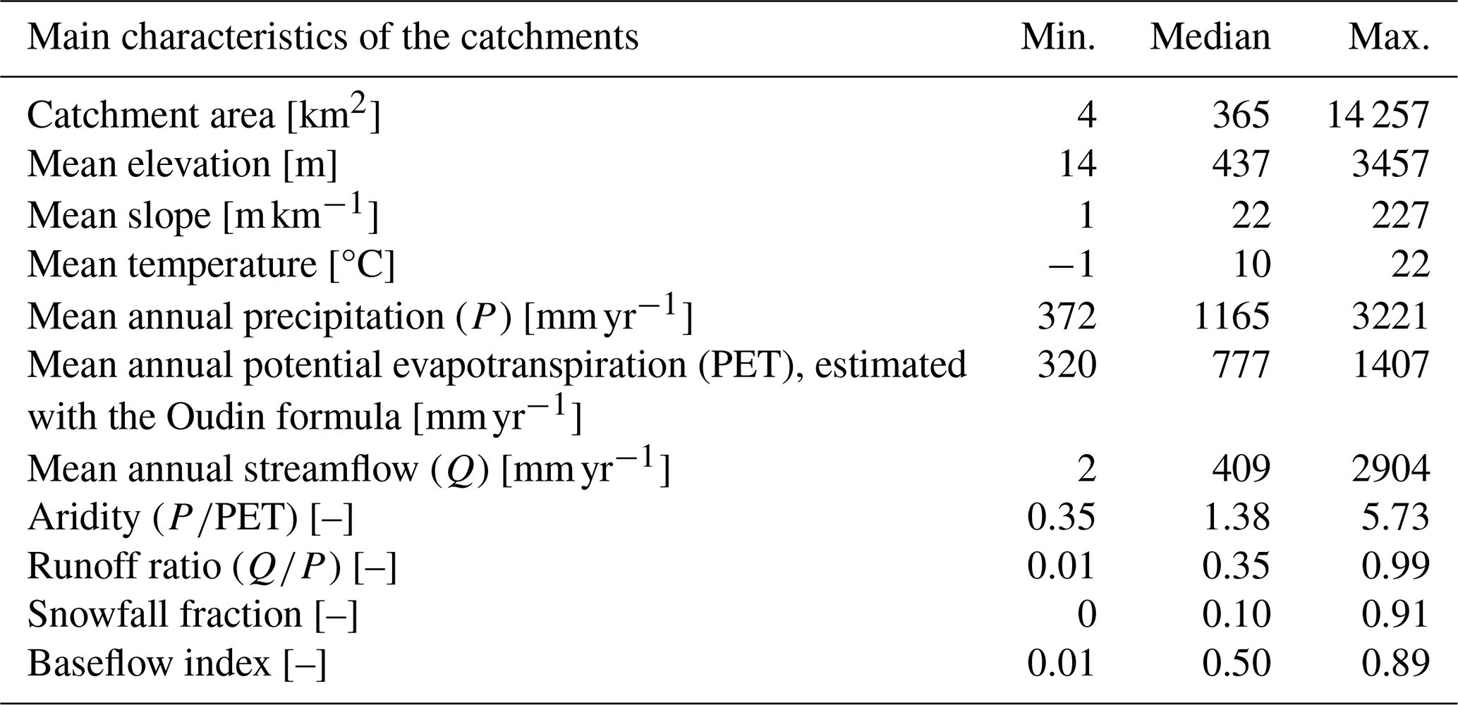
This study is based on the same catchments and hydrometeorological data as Thébault et al. (2025a). In particular, we used the CAMELS data set (Newman et al., 2015; Addor et al., 2017), which provides daily meteorological and streamflow time series for 671 catchments with limited human influence across the contiguous United States (CONUS). CAMELS includes several meteorological forcing products: Daymet (Thornton et al., 2012), Maurer (Livneh et al., 2013), and NLDAS (Xia et al., 2012). In this work, we used only the Daymet product because it provides the required variables (precipitation and temperature) at the highest spatial resolution (1 km×1 km) compared with the other datasets (12 km×12 km), and has shown better performance in past large-sample hydrologic studies (e.g. Kratzert et al., 2021; Sawadekar et al., 2025). Potential evapotranspiration is calculated using the formulation proposed by Oudin et al. (2005). This equation was chosen for its simplicity, as it requires only daily air temperature and extraterrestrial radiation (a function of Julian day and latitude), and because it was developed and tested with conceptual models, which aligns with the modelling framework used here (see Sect. 2.2). Following Knoben et al. (2020), the number of catchments was reduced to 559 by excluding catchments with large area discrepancies between the provided polygons and reference values, as well as catchments that fall outside the water and energy limits on a Budyko plot. From these 559 catchments, a final subset of 544 catchments was retained for the comparative analyses presented in this study. The remaining catchments were excluded due to model failures or because sampling uncertainties could not be computed consistently across all modelling approaches (see Appendix B for details). Figure 1 provides a map of the 544 catchments retained for analysis, and Table 1 summarizes some of their key attributes from the CAMELS dataset.

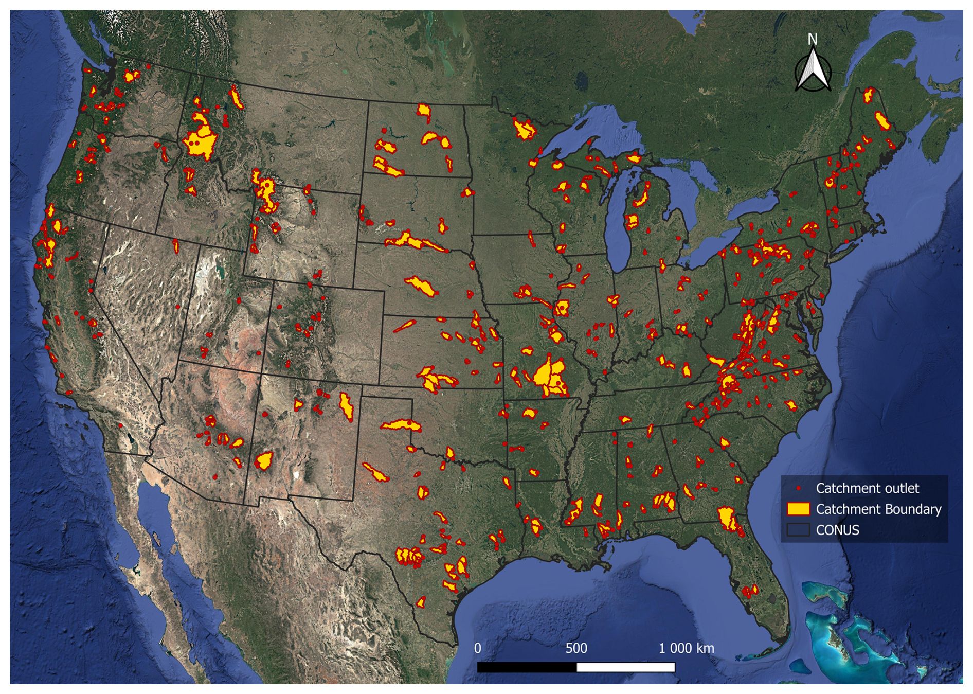
Figure 1 Location of the 544 catchments selected for this study, using state boundaries from the “North American Atlas – Political Boundaries” (Commission for Environmental Cooperation, 2022) and the basemap derived from “Google Satellite”, available through QGIS via the QuickMapServices plugin. Figure based on Thébault et al. (2025a).

Table 1 Statistical summary of some of the key attributes available in the CAMELS data over the 544 catchments selected for this study.

2.2 Hydrological model framework: FUSE

For this study, we use the Framework for Understanding Structural Errors (FUSE) developed by Clark et al. (2008). FUSE is a modular framework that enables the construction of new hydrological model structures from different modules. FUSE is based on four existing conceptual models (Variable Infiltration Capacity, VIC; Precipitation Runoff Modelling System, PRMS; Sacramento Soil Moisture Accounting, SAC-SMA; and TOPMODEL), which were decomposed into individual model components that can be used interchangeably in a general model template.

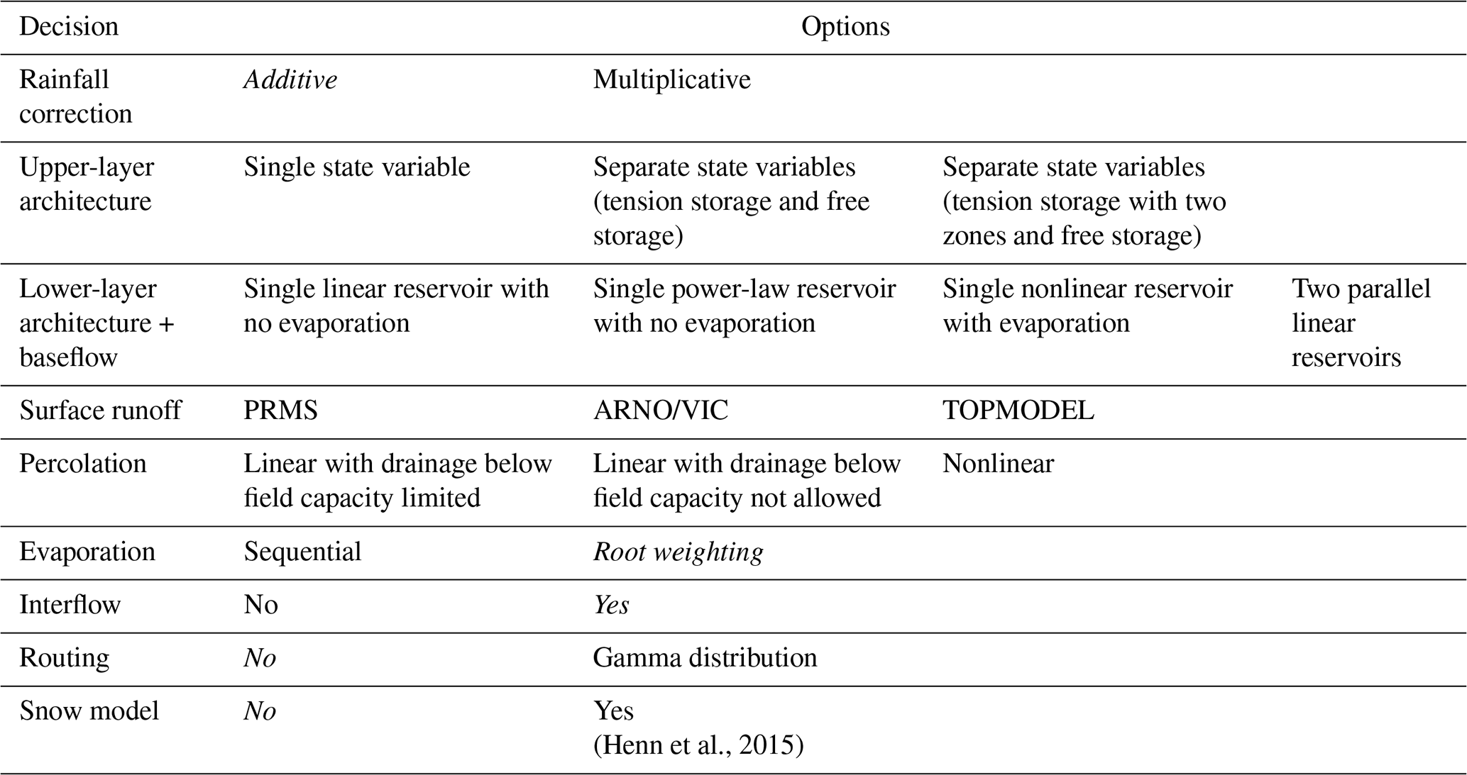
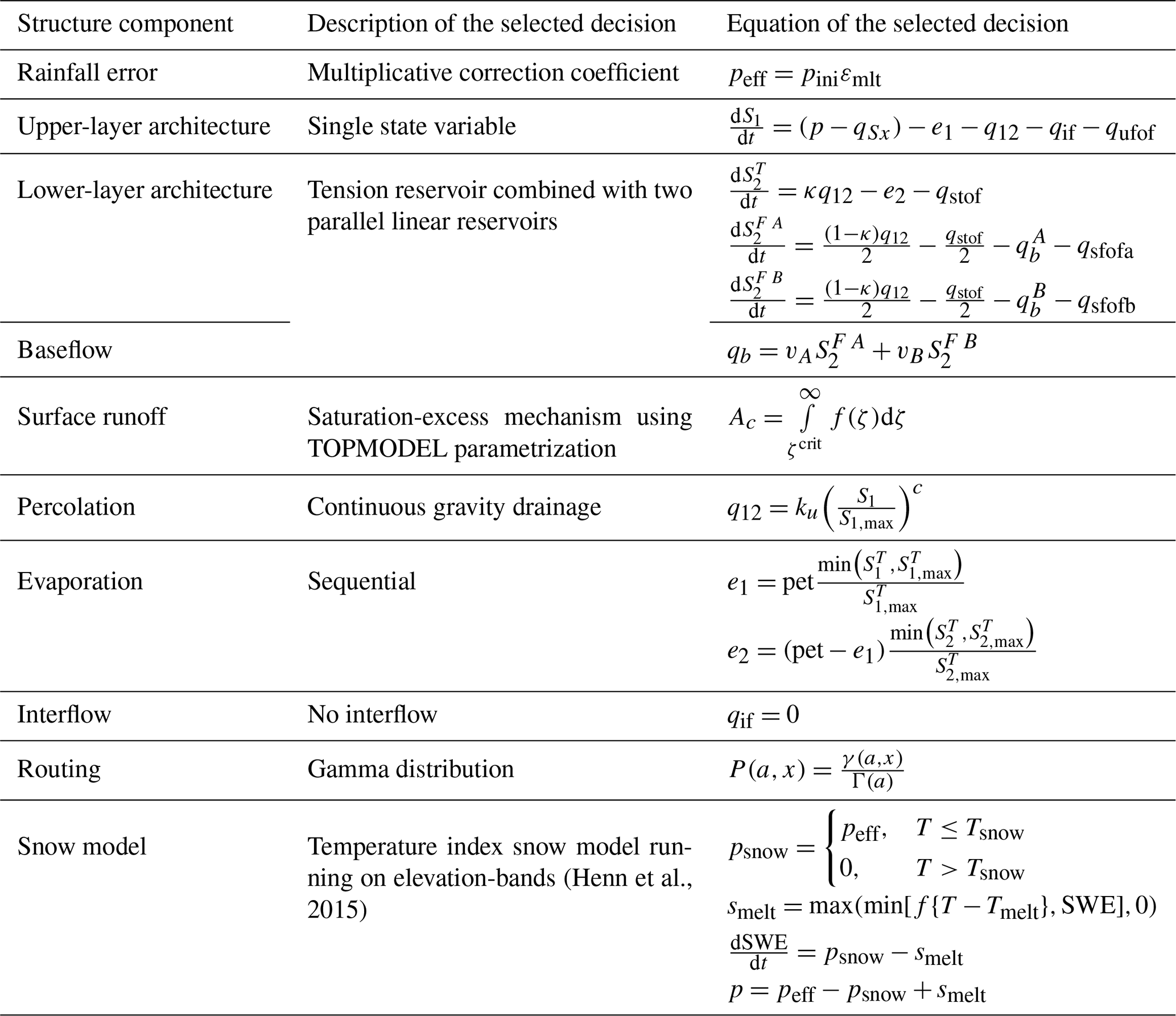
FUSE is designed to enable the investigation of the structural uncertainties and errors inherent in hydrological models by allowing modellers to test different model decisions. In total, more than 3000 structures can be generated using this modular modelling framework. For this study, we focus on the 78 original configurations proposed by Clark et al. (2008). These model structures were created by combining different formulations of the state equations for the upper layer, lower layer and baseflow, percolation, and surface runoff. All other decisions are set to their default values to reduce computational costs and limit the size of the hydrological ensemble to a manageable number. As described in Henn et al. (2015), FUSE was also coupled with a temperature-index snow model based on the Snow-17 formulation (Anderson, 2006). Table 2 summarizes the different decisions in FUSE. Considering the options outlined in each row of Table 2, a total of $\mathrm{3}\times \mathrm{4}\times \mathrm{3}\times \mathrm{3}\times \mathrm{1}\times \mathrm{1}=\mathrm{108}$ model structures is possible. However, as certain combinations of options are not functional, a total of 78 model structures was considered in this analysis. It should be noted that the four parent FUSE configurations (VIC, PRMS, SAC-SMA and TOPMODEL) are included within the 78 structures. Although the 78 model structures provide a broad exploration of conceptual structural decisions within FUSE, they share several common characteristics: all models are lumped, operate at a daily time step, use identical forcing data, and are bucket-style. While this design enables a controlled comparison of structural choices, it does not span fundamentally different modelling paradigms (e.g., fully distributed or data-driven approaches), which may limit the overall structural diversity of the ensemble and could limit the benefits of multi-model approaches (Winter and Nychka, 2010).

Table 2 Model decisions available in FUSE. The options in italics correspond to options that are available in FUSE but not considered in this study.

2.3 Model calibration

The parameters of each of these 78 structures (between 15 and 20 depending on the selected decisions) are calibrated for each catchment using up to 10 000 iterations (e.g., Duan et al., 1994; Tolson and Shoemaker, 2007; Feyen et al., 2008; Lan et al., 2020) of the shuffled complex evolution approach (Duan et al., 1993) to maximize a composite criterion (Garcia et al., 2017):

$$\begin{array}{}\text{(1)}& {\text{KGE}}_{\text{comp}}={\displaystyle \frac{\text{KGE}\left(Q\right)+\text{KGE}(\mathrm{1}/Q)}{\mathrm{2}}}\end{array}$$

where KGE, the Kling-Gupta efficiency (Gupta et al., 2009), is given by:

$$\begin{array}{}\text{(2)}& \text{KGE}=\mathrm{1}-\sqrt{(r-\mathrm{1}{)}^{\mathrm{2}}+(\mathit{\alpha }-\mathrm{1}{)}^{\mathrm{2}}+(\mathit{\beta }-\mathrm{1}{)}^{\mathrm{2}}}\end{array}$$

with r the correlation coefficient, α the ratio of standard deviations, and β the ratio of the means (i.e. the bias) between simulated and observed time-series.

In hydrology, the KGE is typically calculated on streamflow time series without transformation, i.e. as KGE(Q). When used as an objective function for calibration, it is particularly sensitive to high-flow values, often at the expense of low flows (Pushpalatha et al., 2012; Garcia et al., 2017). A common alternative to reduce the influence of high-flow values is to apply a transformation of the time series (e.g., square root, box-cox, inverse). However, Thirel et al. (2024) showed that such an approach only targets a different part of the hydrograph, without successfully capturing the full range of streamflow. This is a known limitation of using a single metric (e.g., Booij and Krol, 2010; Clark et al., 2021). To address this limitation, multi-objective algorithms can be used to better account for multiple facets of streamflow behaviour (e.g. Gupta et al., 1998; Efstratiadis and Koutsoyiannis, 2010; Kollat et al., 2012; Zhang et al., 2018). Such approaches aim to identify trade-offs among competing objectives by approximating a Pareto front rather than a single optimum. An alternative approach is to combine several metrics into a single objective function – here referred to as a composite metric (e.g. Garcia et al., 2017; Hallouin et al., 2020; Thébault et al., 2024). Although this method presents some limitations, such as the loss of some information due to dimensionality reduction or the subjectivity through the weights applied to the different metrics, it typically requires fewer model evaluations because it only needs to converge to a single optimum instead of determining trade-offs with the Pareto front (Efstratiadis and Koutsoyiannis, 2010; Mai, 2023).

In this work, we therefore use a composite metric for the calibration and evaluation of hydrological models, as it provides a good compromise between multi-objectivity and computation time. It aims to provide a balance between high-flow and low-flow (Eq. 1). This metric has already been applied in the literature and has shown benefits compared to traditional single-objective approaches or other combinations of criteria (Garcia et al., 2017).

Each model is calibrated for each catchment over the period 1989–1998 (calendar year), including both relatively wet and dry years, with a preliminary two-year warm-up period (1987–1988) preceding calibration. These periods were selected to maximize the number of catchments with sufficiently complete streamflow time series while maintaining consistency with previous large-sample CAMELS-based studies (e.g. Knoben et al., 2020).

2.4 Model evaluation

The models and multi-model approaches are evaluated over the period 1999–2009 (calendar year), including both relatively wet and dry years. The evaluation framework is divided in three parts: (1) a comparison of performance, (2) an analysis of sampling uncertainty, and (3) an assessment of model equivalence.

2.4.1 Performance

The performance is assessed with the composite metric KGE_comp (Eq. 1).

2.4.2 Sampling uncertainty

We evaluate the robustness of the performance score – defined here as the consistency of model skill across different temporal evaluation regimes – by accounting for sampling uncertainty (Clark et al., 2021; Lamontagne et al., 2020). Specifically, sampling uncertainty refers to the dependency of performance score values, such as NSE and KGE, on the data used for their calculation. This effect is especially pronounced in catchments without strong seasonality in their streamflow regimes, where much of the model error may be concentrated in just a few time steps. Sampling uncertainty can be addressed using bootstrapping methods to provide an estimate of the uncertainty range of a model's performance for a given catchment (see, e.g., Clark et al., 2021). For this study, sampling uncertainty in performance metrics is quantified using the gumboot R package (Clark and Shook, 2021), following the default bootstrap procedure described by the authors. Specifically, the method resamples non-overlapping blocks of complete water years with replacement to generate 1000 synthetic hydrographs, preserving within-year autocorrelation and seasonality. Sampling uncertainty is expressed as the interval between the 5th and 95th percentiles of the resulting bootstrap distribution. Note that the KGE_comp is not implemented in the current version of gumboot; we therefore extended the package to include this metric for the present analysis.

2.4.3 Performance equivalence

Knoben et al. (2025) showed that many models often exhibit performances falling within the sampling uncertainty range of the model that initially achieves the highest KGE score in a given catchment (i.e., within the range of the 5th and 95th percentile range of the bootstrap distribution of the top-performing model). In such cases, the models are considered equivalent. Here, we apply this method to test the equivalence between multi-model approaches.

2.5 Multi-model approaches

2.5.1 Performance benchmark

We establish our benchmark by selecting, from the ensemble of 78 models, a single model across all catchments. Specifically, the benchmark is defined as the model with the highest median KGE_comp value over the calibration period and across the 544 catchments. It should be noted that while we select a single model for all catchments as our benchmark, the process of how it is selected differs from traditional “one-size-fits-all” approaches, which are typically based on legacy or convenience selections (Addor and Melsen, 2019). Our approach instead selects a single model based on proven performance superiority compared to the 77 considered alternative FUSE models and can therefore be viewed as a multi-model approach. The benchmark serves as a stringent baseline against which the value of more complex multi-model strategies can be assessed. Therefore, the benchmark is not intended to represent a typical legacy model choice, but rather to provide either a high boundary for single-model modelling and a reference for multi-model experiments. Additional details on the benchmark structure and its performance distribution are provided in Appendix A (Fig. A1 and Table A1).

2.5.2 Multi-model mosaics

Multi-model mosaics aim to assign a single suitable model taken from a larger model ensemble to each individual catchment. Here, we explore two approaches for building this spatial model mosaic: one based on performance only (Sect. 2.5.2, Mosaic based on performance), and the other on performance-equivalence (Sect. 2.5.2, Mosaic based on performance-equivalence).

Mosaic based on performance

One possible implementation of the multi-model mosaic approach is to select a single model per catchment based on aggregated performance metrics such as KGE or NSE (Knoben et al., 2020; Spieler et al., 2020; Mai et al., 2022; Thébault et al., 2024). In this study, we replicate such a performance-based mosaic approach by selecting, for each catchment, the model with the highest KGE_comp value during the calibration period. Further details on the spatial distribution and frequency of selected models are provided in Appendix A (Fig. A2).

Mosaic based on performance-equivalence

Another possible implementation of the multi-model mosaic approach uses the principle of performance-equivalence introduced by Knoben et al. (2025) to account for sampling uncertainty in performance scores. By assessing which models are equivalent to the top-performing one (i.e., whose scores fall within the sampling uncertainty of the top-performing model) in each catchment, it is possible to minimise the number of models required across the domain. This task is carried out using a linear programming algorithm from the lpSolve R package (Csárdi and Berkelaar, 2024) by solving a set cover type problem. In this study, the mosaic based on performance-equivalence is derived from the ensemble of 78 models, where sampling uncertainty and model selection are guided by the KGE_comp metric over the calibration period. The purpose of minimizing the number of models is to promote parsimony and spatial coherence. While many structures may be statistically equivalent, in term of performance metric value, in a given catchment (Fig. A3), selecting a different model in each location may lead to a highly fragmented mosaic with limited interpretability. Across the domain, this procedure reduces the 78 candidate structures to only eight distinct models required to cover all catchments (Fig. A4). Additional methodological details and supporting results are provided in Appendix A (Figs. A3 and A4).

2.5.3 Multi-model combinations

Multi-model combinations aim to leverage the potential complementarity of hydrological models within a given catchment by averaging streamflow outputs from an ensemble of models, thereby improving approximation of the expected hydrologic response and providing insight into uncertainty arising from differences in model structure. In this study, we explore three approaches for constructing such combinations: the first combination uses static weights across time and space (Sect. 2.5.3, Spatially and temporally static combination), the second combination uses weights that are static in time but variable in space (Sect. 2.5.3, Spatially variable and temporally static combination), and the last combination uses weights that change dynamically in space and in time (Sect. 2.5.3, Spatially and temporally variable combination).

Spatially and temporally static combination

A static combination in time and space refers to a single combination of several models used for streamflow predictions in all catchments, with weights that do not change. There are numerous ways to derive the weights for such a setup (see, e.g., Arsenault et al., 2015; Wan et al., 2021; Todorović et al., 2024), with no particular approach appearing to be consistently better than the others. We adopt an approach similar to that of Thébault et al. (2024), who demonstrated the benefits of a simple static combination approach on a large sample of catchments: for a combination of n models among an ensemble of m models, each selected model receives a weight of $\mathrm{1}/n$, and the weight of the other m−n models is set to 0. Thébault et al. (2024) also showed that the performance gain from combining four models is limited compared to the performance that can be achieved by combining three models. In this work, considering all combinations of up to four models (among an ensemble of 78 models) would result in a substantially larger number of possibilities compared to three (${}_{\mathrm{2}}^{\mathrm{78}}C+{}_{\mathrm{3}}^{\mathrm{78}}C+{}_{\mathrm{4}}^{\mathrm{78}}C=\mathrm{1}\mathrm{505}\mathrm{504}$ vs. ${}_{\mathrm{2}}^{\mathrm{78}}C+{}_{\mathrm{3}}^{\mathrm{78}}C=\mathrm{79}\mathrm{079}$ combinations per catchment), which would drastically increase computational cost. To achieve a better balance between computational cost and performance, this study considers only combinations of two or three models (see also Fig. A5, which shows that imposing a three-model limit is acceptable in our case). Note that combinations of size one (i.e. equivalent to a single model) are not included in the search space, although they may yield marginally higher performance in a subset of catchments (see Appendix C). The spatially and temporally static combination is defined as the combination that yields the highest median KGE_comp score over the calibration period across the 544 catchments. The distribution of performance across all tested combinations and identification of the top-performing combination are shown in Appendix A (Fig. A5).

Spatially variable and temporally static combination

This approach recognizes that not every model might be equally appropriate for every catchment and instead selects an optimal combination for each individual catchment. This approach is similar to the previous combination (Sect. 2.5.3, Spatially and temporally static combination), except that the models selected in the combination differ for each individual catchment. In other words, for each of the 544 catchments, we identify the combination of two or three models that yields the highest KGE_comp scores over the calibration period. The diversity of selected combinations and model frequencies are detailed in Appendix A (Figs. A6 and A7).

Spatially and temporally variable combination

The aim of this approach, hereafter called the “dynamic combination”, is to dynamically combine model simulations across time and space – in this case selecting from all 78 models. Therefore, the weight given to each of the 78 simulations varies at each time step and for each catchment. The general principle of the dynamic combination method is to identify past periods with similar hydrological conditions to the current one and define model weights for the current time step based on model performance during those analogous periods. In this study, we adopt the specific implementation used in Thébault et al. (2025a) which involves two chained components run for each time step: (1) a search for past time periods (typically in the calibration period) similar to current conditions (typically in the evaluation period), implemented as a k-nearest-neighbour (k-NN) search based on Mean Absolute Error (MAE) scores between the streamflow simulation representing current conditions and past observations; and (2) a weighting of simulations based on mean MAE scores between each model's simulations and past observations across the identified neighbours. Further methodological details on the dynamic combination framework can be found in Thébault et al. (2025a).

We deviate slightly from the implementation in Thébault et al. (2025a), by allowing the parameters of the dynamic combination – namely, the length of the time window (τ, ranging from 4 to 28 d), the number of nearest neighbours (k, ranging from 1 to 19), and the number of models to combine (m, ranging from 1 to 19) – to vary across catchments (see Fig. A8). These parameters control how the method identifies similar past conditions and determine the weights assigned to individual models. Here, their values are optimized for each catchment to account for spatial heterogeneity. In addition, Thébault et al. (2025a) highlighted that the strength of the dynamic combination comes from using an ensemble calibrated on different objective functions. Here, we deliberately limit the optimization to a single metric (KGE_comp) to ensure that observed differences among approaches reflect their intrinsic combination mechanisms rather than differences in calibration effort or metric alignment.

It should be noted that a major difference between the dynamic combination and the two previous multi-model combination approaches (Sect. 2.5.3, Spatially and temporally static combination and Spatially variable and temporally static combination) is that, in the dynamic combination, models are selected based on their individual performance (78 simulations evaluated) rather than on their combined performance (${}_{\mathrm{2}}^{\mathrm{78}}C+{}_{\mathrm{3}}^{\mathrm{78}}C=\mathrm{79}\mathrm{079}$ simulations evaluated). While adapting the method to evaluate combined performances (e.g., by assessing all possible combinations of two or three models across each neighbour) would be straightforward in principle, it would drastically increase computation time and complexity. Distributions of optimized parameters and model usage patterns are presented in Appendix A (Figs. A8–A10).

2.6 Summary

We test six different multi-model approaches based on an ensemble of 78 models calibrated with KGE_comp, across 544 CONUS catchments. Further details and analyses on each multi-model approach are provided in Appendix A. Table 3 summarizes these experiments, Fig. 2 provides a schematic illustration of the different approaches, and the following points briefly summarize their implementation:

• The benchmark corresponds to a single model (the highest median performance across all catchments) applied everywhere.

• The performance-based mosaic assigns one model per catchment (the top-performing model across each catchment).

• The performance-equivalence mosaic extends this idea by explicitly accounting for sampling uncertainty in performance scores. A linear-programming algorithm identifies the minimum set of equivalent models needed to maintain performance within these uncertainty bounds, yielding a spatially parsimonious mosaic.

• The spatially and temporally static combination selects a single combination of models that is applied to all catchments. All possible combinations of two or three models (${}_{\mathrm{2}}^{\mathrm{78}}C+{}_{\mathrm{3}}^{\mathrm{78}}C=\mathrm{79}\mathrm{079}$ simulations per catchment) are evaluated, and the combination with the highest median performance across catchments is selected. The combination is computed by simple averaging, i.e., assigning equal weights to the selected models.

• The spatially variable and temporally static combination follows the same principle but determines the optimal combination (of two or three models) independently for each catchment.

• The dynamic (i.e., spatially and temporally variable) combination adapts model weights (up to 19 models selected based on individual performance) across space and time based on similarities during past conditions.

Table 3 Overview of the multi-model approaches evaluated in this study. Although the dynamic combination involves up to 19 models, the model selection is based on individual rather than combined performance, reducing its apparent complexity (see Sect. 2.5.3, Spatially and temporally variable combination).

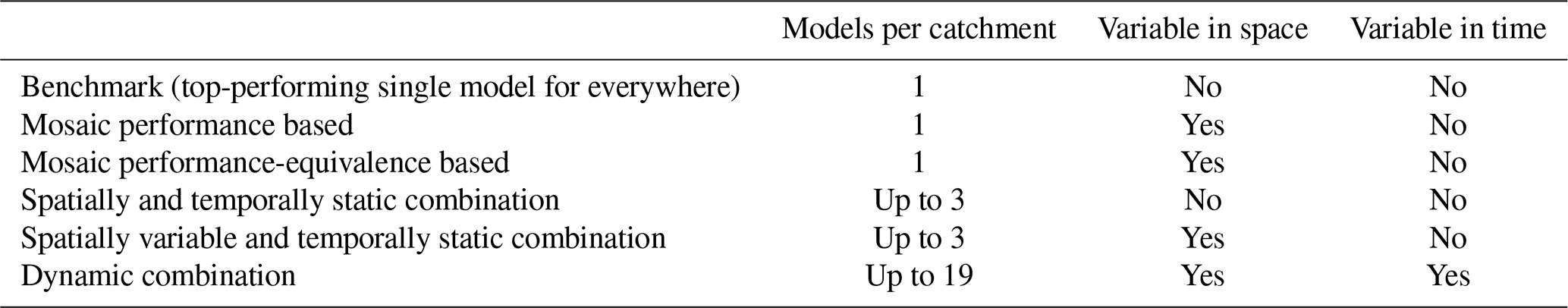
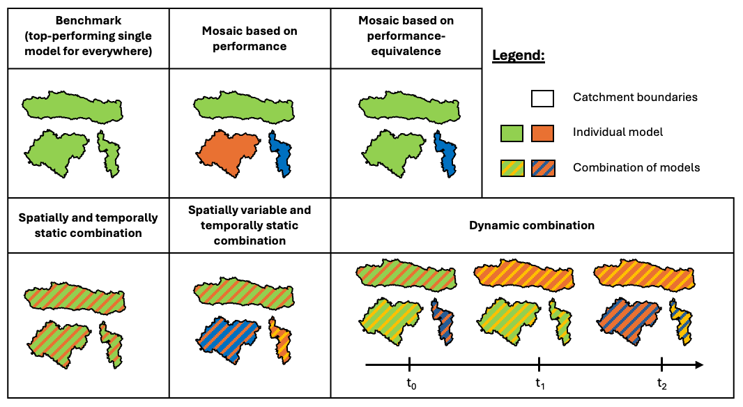
Figure 2 Schematic illustration of the six multi-model approaches tested. Each colour represents a model, e.g. the benchmark uses the same model everywhere, whereas in the mosaic approaches the selected model can be different for each catchment. Note that when we compare the two mosaic approaches (top row), the orange catchment becomes green, meaning that green model is equivalent to the orange one in that specific catchment. Hatched areas (bottom row) indicate combinations of models. The x axis in the bottom right plot represents time, showing that the combination of models can vary on a per-timestep basis.

3 Results

In the following sections, we first examine the overall behaviour of the FUSE ensemble and the single-model benchmark (Sect. 3.1). We then compare the different multi-model approaches in terms of their predictive performance (Sect. 3.2.1) and the associated sampling uncertainty (Sect. 3.2.2). Finally, we assess whether the multi-model approaches are equivalent across the catchments (Sect. 3.3). This analysis aims to answer three main questions:

• (i)

  How does each multi-model approach perform relative to the single-model benchmark across a large sample of catchments?

• (ii)

  How robust are these performance differences given sampling uncertainty?

• (iii)

  To what extent do different multi-model approaches provide equivalent performance across space?

3.1 FUSE model ensemble and benchmark

Figure 3 shows the KGE_comp metric of the individual FUSE models over both calibration and evaluation periods. The spread demonstrates substantial performance differences attributable to model structure, with median values (i.e. CDF at 0.5) varying from 0.59 to 0.82 during the calibration period and from 0.29 to 0.69 during the evaluation period, depending solely on the structure employed. The benchmark, defined as the model achieving the highest median KGE_comp across catchments during the calibration period, is highlighted in bold. This model also maintains one of the highest performance distributions during the evaluation period. However, this does not mean that it systematically outperforms all other models in every catchment (result not shown here for simplicity, but valid for both the calibration and evaluation period). The per-catchment performances of the benchmark model, presented in Fig. 4, exhibit a spatial pattern typical of streamflow modelling across CONUS (e.g., Newman et al., 2015; Knoben et al., 2020), with lower performance scores in the drier central area. While it is well documented that KGE (and related composite metrics) are influenced by streamflow variability and therefore are not directly comparable across locations (Schaefli and Gupta, 2007; Knoben et al., 2019; Williams, 2025), these maps provide a general sense of model skill and enable per-catchment comparison between the calibration and evaluation periods. Details about the model selected as a benchmark are given in Table A1. As a reminder, this benchmark aims to provide either a high boundary for single-model modelling and a reference for multi-model experiments, rather than a simple baseline based on legacy choices. However, for transparency, the four parent FUSE configurations corresponding to VIC, PRMS, SAC-SMA, and TOPMODEL are explicitly highlighted in grey in Fig. 3, allowing readers to assess their relative performance within the full ensemble.

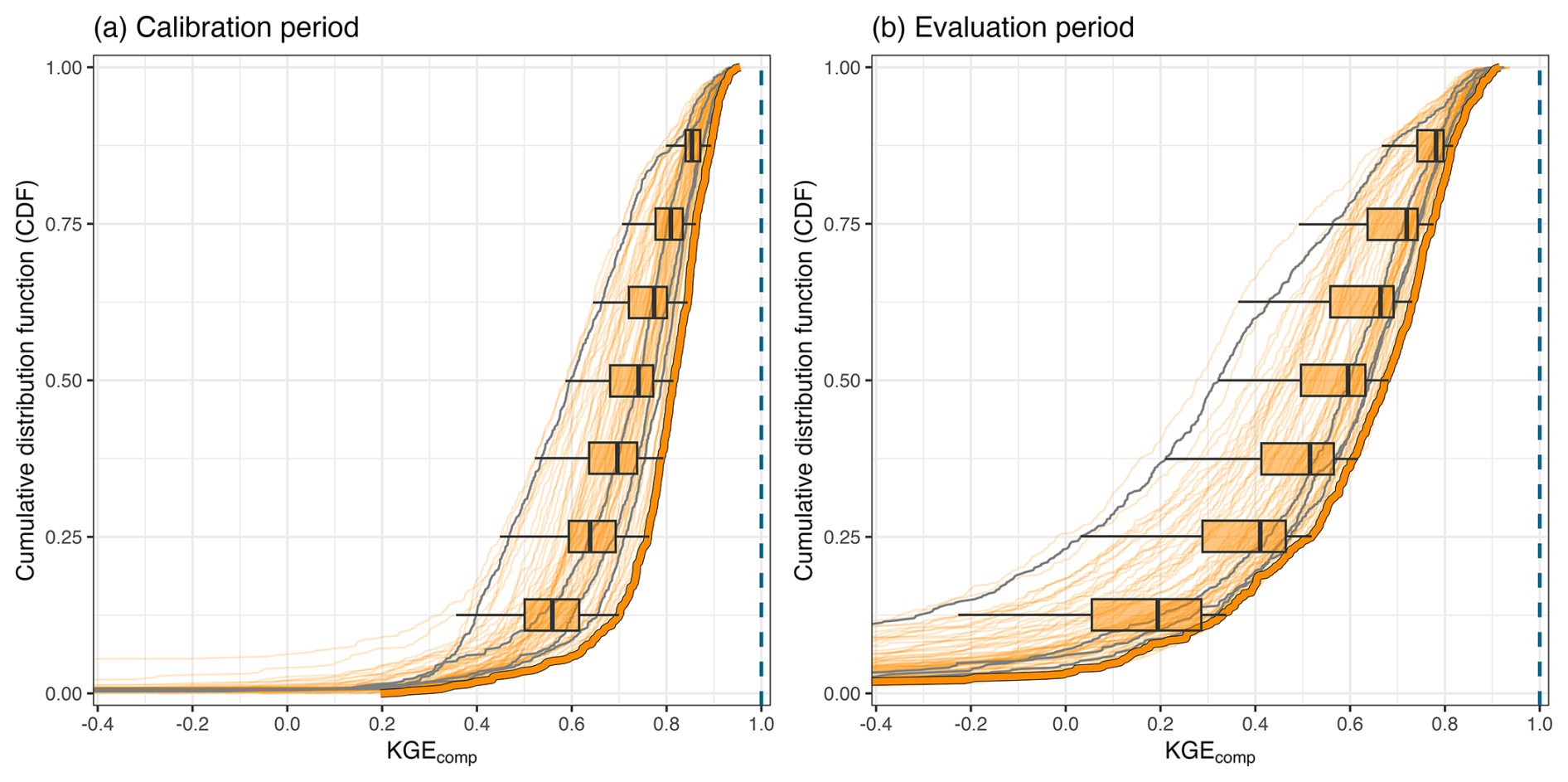
Figure 3 Distribution of the performance score KGE_comp of the individual FUSE models (78 structures) across the 544 catchments during (a) the calibration and (b) the evaluation period. A slight transparency has been applied to avoid problems of misinterpretation due to line overlaps. The bold line highlights the benchmark, i.e., the top-performing model based on median KGE_comp value across all catchments for the calibration period. The grey lines show the four parent FUSE configurations (VIC, PRMS, SAC-SMA, and TOPMODEL) The boxplots illustrate the ensemble spread (differences linked to model structure) for different values of the cumulative distribution function (CDF): 0.125, 0.25, 0.375, 0.5, 0.625. 0.75 and 0.875. The dashed blue line indicates the optimum value of the KGE_comp score, i.e. 1.

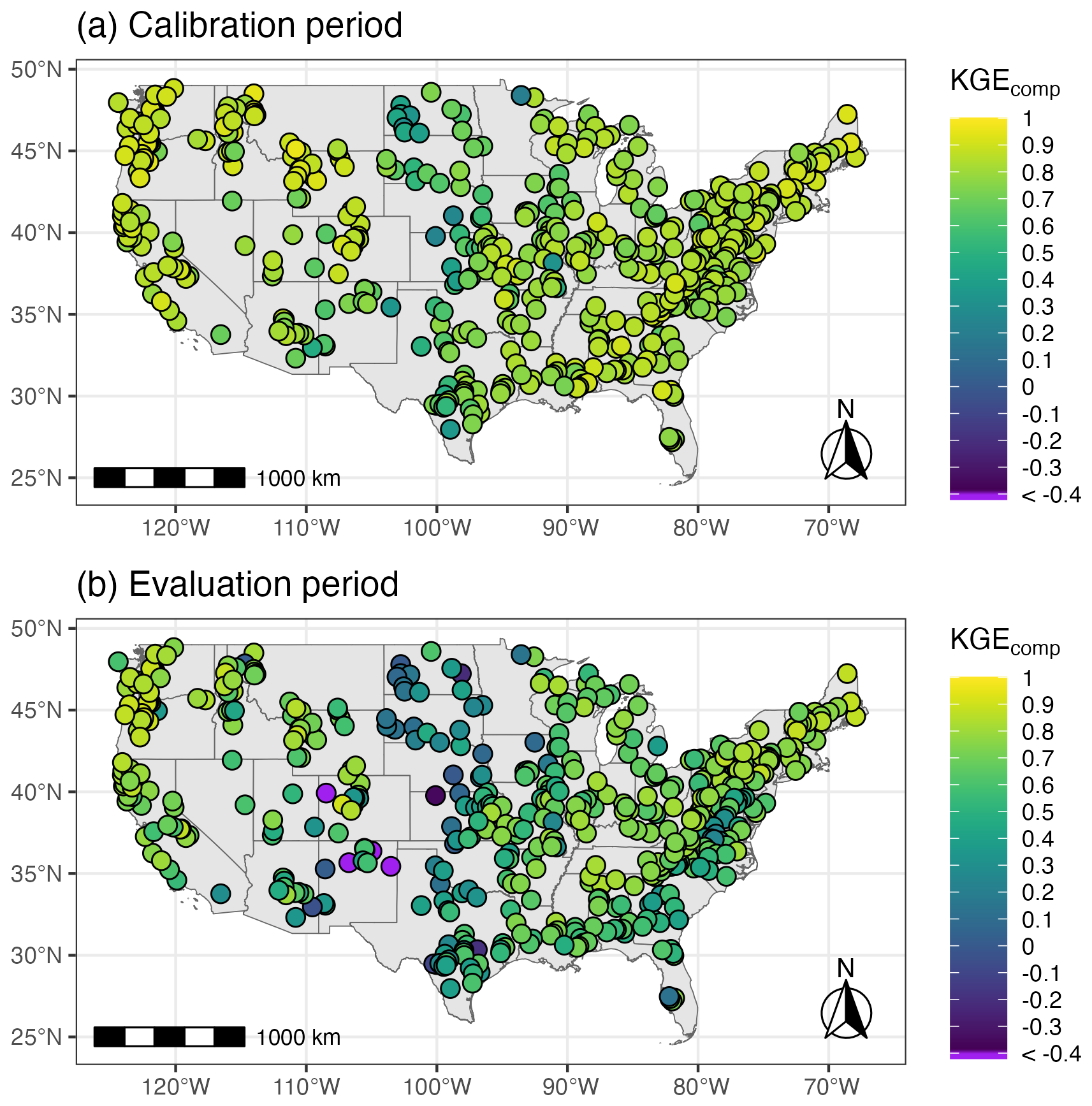
Figure 4 Spatial distribution of the performance score KGE_comp of the benchmark model across 544 catchments during (a) the calibration and (b) the evaluation period. The benchmark corresponds to the top-performing model based on the median KGE_comp value across all catchments during the calibration period.

3.2 Comparison of the multi-model approaches

3.2.1 Performance

Figure 5 presents a comparison of performance scores of all multi-model approaches with the benchmark model for the composite criterion KGE_comp over the evaluation period. Overall, all various modelling approaches tested here yield similar performance scores.

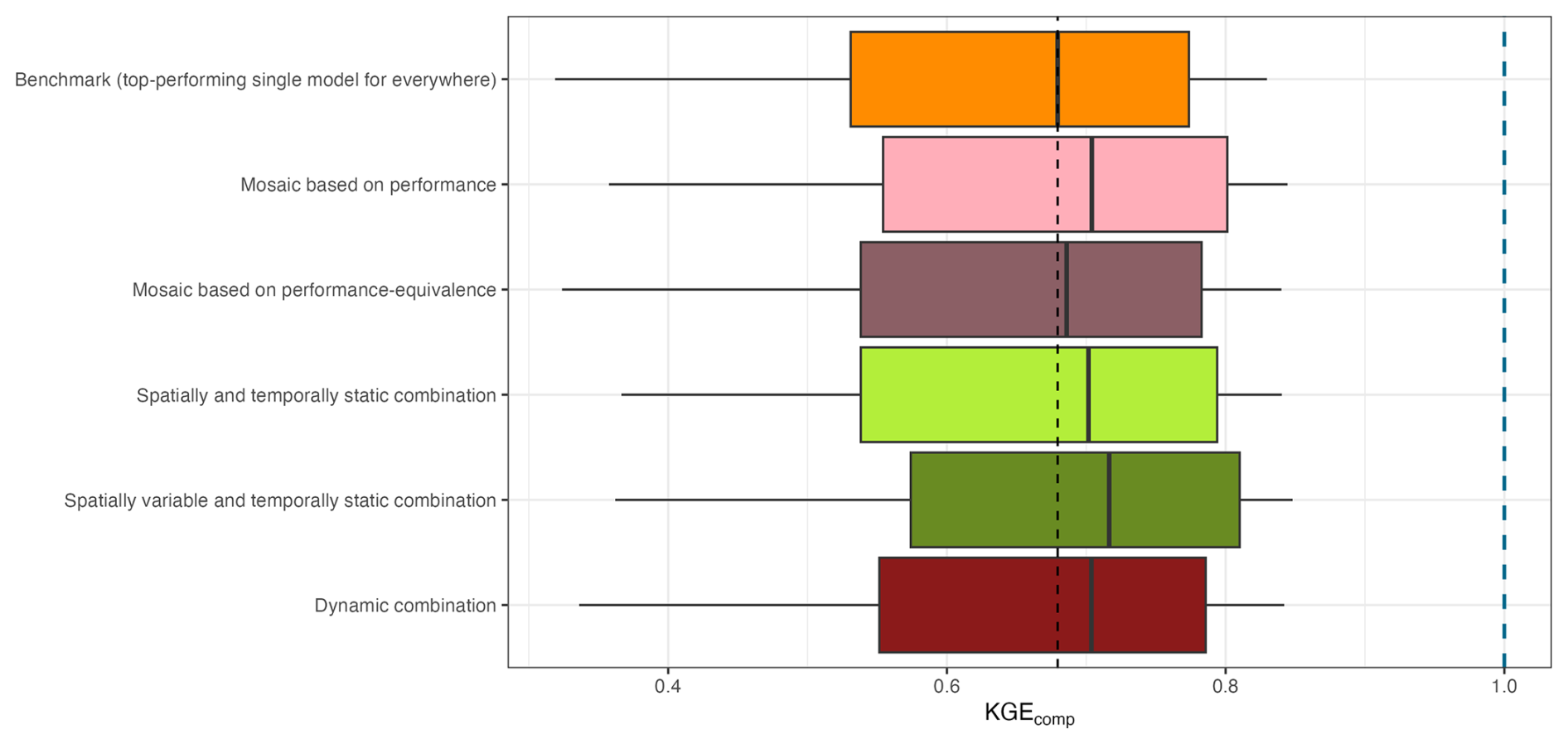
Figure 5 Boxplot of performance scores, KGE_comp, over the evaluation period for the different multi-model approaches. The boxplots represent the 10 %, 25 %, 50 %, 75 % and 90 % quantiles. The dashed black line indicates the median value of the benchmark. The dashed blue line highlights the optimal value of KGE_comp.

Surprisingly, the benchmark (orange) – a single model applied across all catchments – achieves a score distribution that is very close to those of multi-model approaches (slightly lower) with a median value of 0.68. However, unlike typical “one-size-fits-all” strategies, the model selected here was not chosen based on legacy or convenience. Although the outcome is the same (one model for all catchments), it is chosen on performance across a broad spatial domain (544 catchments) from a large ensemble of models (78 structures). In this sense, the benchmark stems from an initial multi-model experiment, where all structures were candidates to become the benchmark. Its comparison with purely multi-model methods points to a promising pathway toward developing a robust single-model solution if the selection method is carefully considered.

The multi-model mosaic approaches do not exhibit a substantial improvement in performance compared to the single-model benchmark across the sample of catchments. The mosaic based purely on performance (light pink) provides an increase in the median performance of 0.02 (to 0.70) and also benefits the other quantiles considered. The mosaic approach based on performance-equivalence (dark pink) shows scores more similar to the benchmark model (with a median of 0.69 and similar quantiles). This result is consistent with Fig. A4, where the model structure that was selected as the benchmark model is used by nearly 80 % of the catchments for the mosaic based on performance-equivalence.

The multi-model combination approaches also do not exhibit performance that substantially improves upon the single-model benchmark. The spatially and temporally static combination (light green) provides a distribution of performance scores very close to those obtained with a performance-based mosaic approach (median of 0.70 and similar quantile distributions), even though the model choice does not vary spatially. This result thus highlights that there are some benefits of combining several models – i.e., using an ensemble of models rather than a single one. As expected, enabling a degree of freedom in space, with the spatially variable and temporally static combination (dark green), leads to slightly better results over the evaluation period (median of 0.72). This approach achieved the highest performance among all the multi-model approaches tested, although the differences remain small. Although more complex, the dynamic combination (red) does not provide the highest scores (median of 0.70) and leads to a performance distribution similar to what can be obtained with a static combination in time and space (light green) or a mosaic based on performance (light pink). This result is discussed in Sect. 4.3, which examines why the dynamic combination does not outperform other multi-model approaches.

To complement the domain-wide performance summaries, Fig. 6 illustrates the spatial distribution of KGE_comp scores for each multi-model approach and provides a comparison with the benchmark model. The maps reveal that all multi-model approaches produce broadly consistent spatial patterns, similar to those found in the literature for streamflow modelling across CONUS (e.g, Newman et al., 2015; Knoben et al., 2020). Differences to the benchmark are mostly limited in magnitude, with predominantly light blue tones overall, indicating a slight overall improvement (consistent with the previous results). However, a few outliers can be observed, showing large improvements or deteriorations for specific catchments. These strong variations mostly occur in catchments where modelling is initially challenging (i.e., where performances are low in Fig. 4), likely reflecting some degree of overfitting during calibration in poorly constrained catchments. This interpretation is supported by Fig. 6a: the performance-based mosaic cannot perform worse than the benchmark during calibration by construction, yet during evaluation it sometimes yields substantially poorer performance, illustrating how calibration-time gains can fail to generalize.

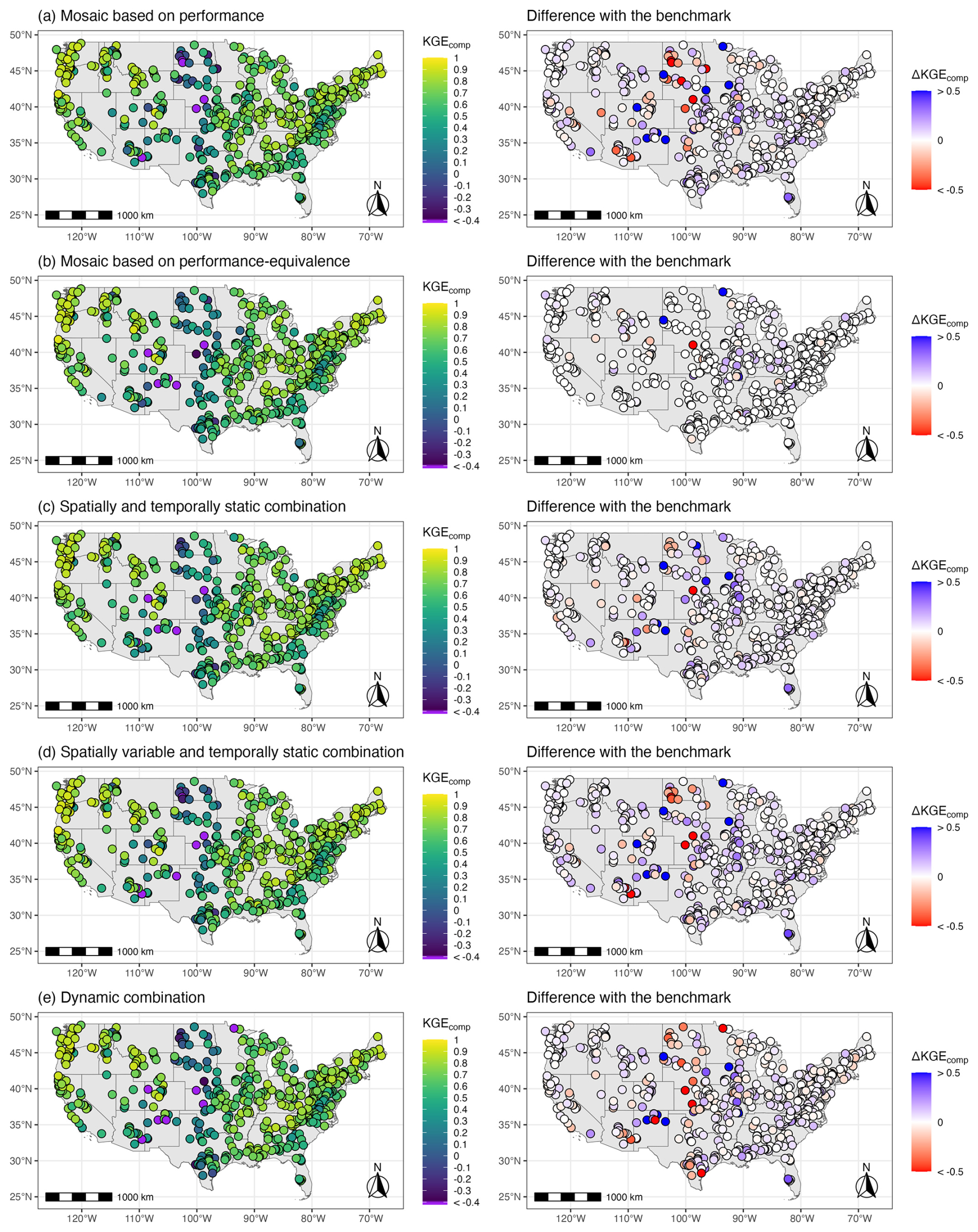
Figure 6 Spatial distribution of the performance score KGE_comp of the different multi-model approaches across 544 catchments over the evaluation period. The difference with the benchmark is also shown in the right column; blue colours indicate better performance with the multi-model approach, while red colours indicate worse performance.

3.2.2 Sampling uncertainty

The purpose of sampling uncertainty is to assess the sensitivity of performance scores (here, KGE_comp) to the specific period over which they are calculated (here, the evaluation period). Figure 7 presents a comparison of the sampling uncertainty associated with KGE_comp for the various multi-model approaches, calculated using the gumboot package. For each multi-model approach and each catchment, we computed the 5th–95th percentile uncertainty interval around the KGE_comp scores using bootstrap resampling. In practical terms, narrower intervals (i.e., values closer to zero) indicate more robust scores, meaning that the KGE_comp values vary little with the choice of the time period used for their calculation. Such comparisons are useful to assess whether the differences in KGE_comp among multi-model approaches exceed the uncertainty in the scores themselves.

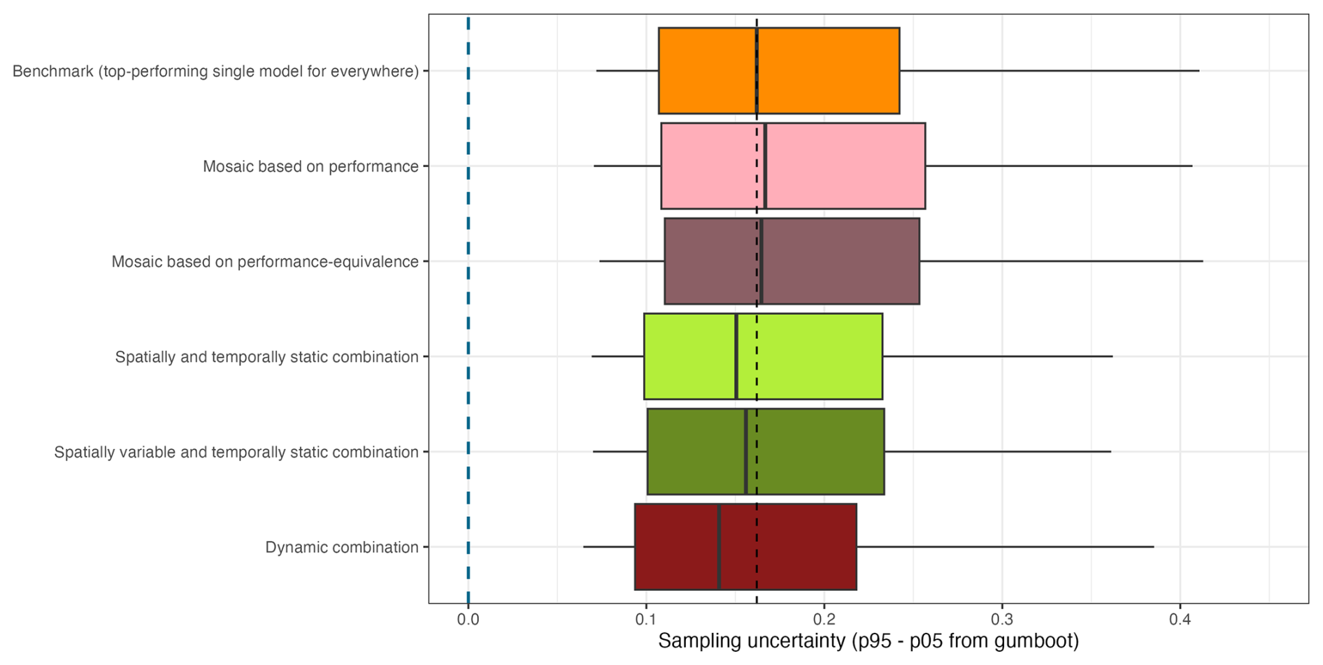
Figure 7 Boxplot of sampling uncertainty surrounding the performance score KGE_comp over the evaluation period for the various multi-model approaches. The boxplots represent the 10 %, 25 %, 50 %, 75 % and 90 % quantiles. The dashed black line indicates the median value of the benchmark. The dashed blue line highlights the optimal value of sampling uncertainty range.

Differences in sampling uncertainty across the approaches are minor. Nevertheless, Fig. 7 shows slightly lower (i.e. better) sampling uncertainty for combination approaches (light green, dark green and red) compared with the mosaic approaches (light and dark pink) or the single-model benchmark (orange). This tendency likely reflects that selecting a single model for each catchment (or across all catchments) increases the risk of choosing a model that appears to perform well at first glance (i.e., during calibration) but is highly sensitive to the evaluation period (i.e., lacks robustness). In contrast, combination approaches tend to dampen this effect because they aggregate multiple models. Note that the pattern in Fig. 7 (sampling-uncertainty analysis) differs from that in Fig. 5 (performance analysis): the top-performing approach is not the least uncertain. In other words, although the spatially variable and temporally static combination approach achieves the highest evaluation performance, its scores do not exhibit the lowest uncertainty among all approaches, indicating that its apparent superiority may be less robust across time. By contrast, the dynamic combination approach yields the lowest sampling uncertainty; this likely occurs because the time-varying weights in the dynamic combination adapt to shifts in hydro-climatic conditions, and, as such, the dynamic combination method is more resilient to differences in the temporal samples that are used to quantify sampling uncertainty.

Although the multi-model combination methods tend to exhibit lower sampling uncertainty when aggregated across all catchments, this does not necessarily hold on a per-catchment basis. Figure 8 illustrates this point by comparing the sampling uncertainty of each multi-model approach against that of the benchmark model for each catchment. The percentages shown in each panel indicate the proportion of catchments where the multi-model approach has lower (bottom-right value) or higher (top-left value) sampling uncertainty than the benchmark. For example, the dynamic combination reduced sampling uncertainty compared to the benchmark for about 63 % of catchments but increased it for 37 % (Fig. 8e), indicating that improvement is not absolute. This result highlights that while multi-model combinations can improve overall sampling uncertainty (Fig. 7), they do not systematically yield more robust scores across all catchments. Note that for multi-model mosaic approaches, the percentages do not sum to 100 %. This reflects the fact that, in multi-model mosaic approaches, the model used as the benchmark can also be selected to simulate a given catchment, resulting in identical sampling uncertainty for those cases (3 % of the catchments for the mosaic based on performance, and 79 % for the mosaic based on performance-equivalence). Most of the larger degradations occur in initially poor-performing catchments (blue and purple colours).

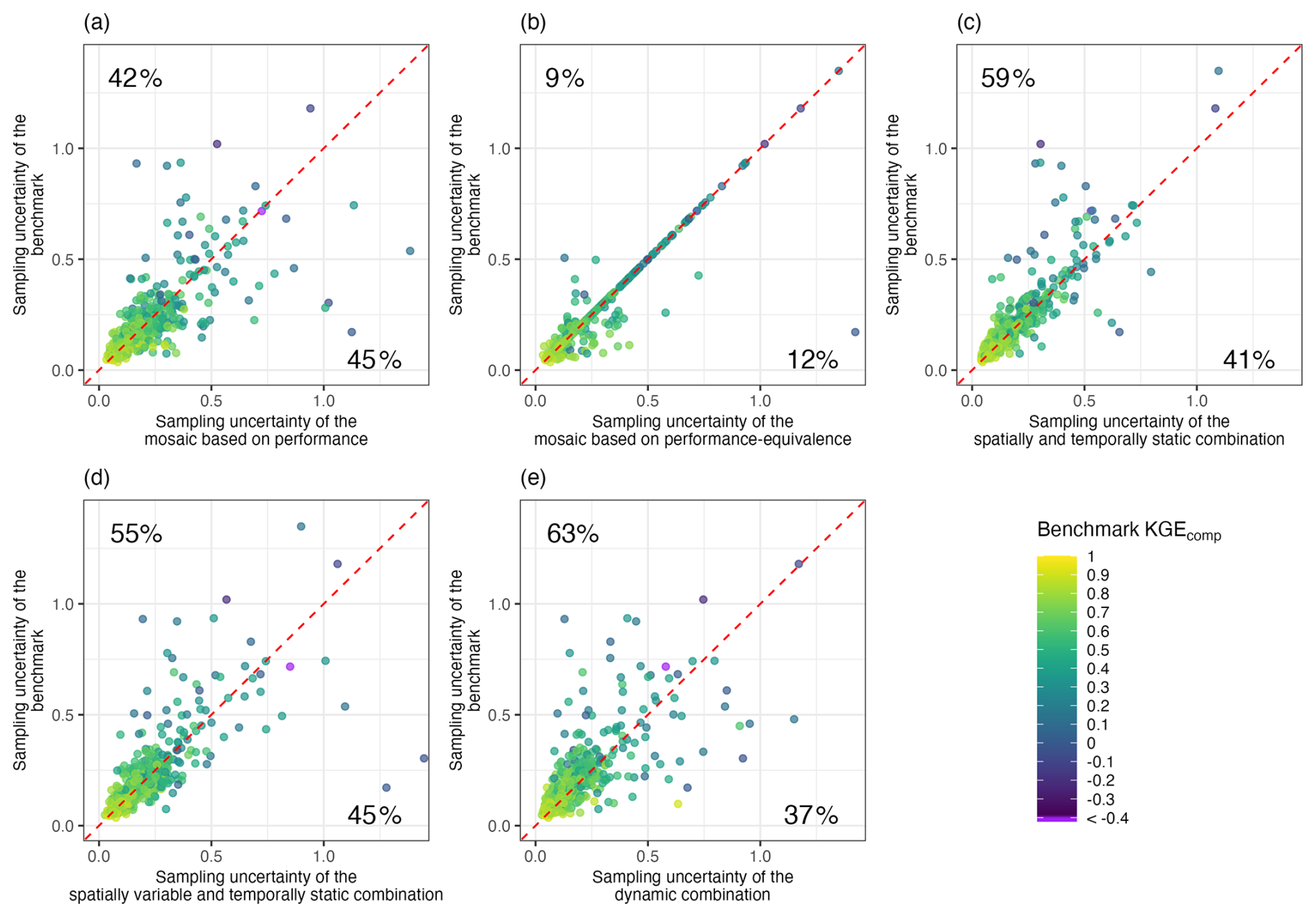
Figure 8 Scatter plot comparing sampling uncertainty (defined as the difference between the 5th and 95th percentiles of the KGE_comp bootstrap distribution) between the benchmark and the multi-model approaches: (a) mosaic based on performance, (b) mosaic based on performance-equivalence, (c) spatially and temporally static combination, (d) spatially variable and temporally static combination, and (d) dynamic combination. The dashed red line indicates equality. Dots below the 1:1 line indicate an increase in sampling uncertainty (i.e. a degradation), whereas dots above the line indicate a decrease (i.e. an improvement) resulting from the multi-model approach relative to the benchmark. The numbers indicate the percentage of catchments that fall on each side of the 1:1 line. The colour scale indicates the initial KGE_comp performance of the benchmark.

3.3 Equivalence

In this section, we assess whether the different multi-model methods provide added value that makes them distinguishable from one another. Using the notion of performance-equivalence introduced in Sect. 2.4.3, we determine whether two approaches are effectively indistinguishable for a given catchment – i.e., whether the KGE_comp score of the lower-performing approach lies within the sampling uncertainty interval of the other, here over the evaluation period.

Figure 9 summarizes these equivalence analyses. Overall, the various multi-model approaches are indistinguishable for at least 69 % of the catchments (white bars), regardless of the method considered. In other words, in most catchments, changing the multi-model strategy does not yield statistically meaningful differences in performance. Among the remaining 31 % of catchments, no approach consistently outperforms the others. Each method shows a mixture of improvements (blue bars) and deteriorations (red bars), with no strategy achieving systematic superiority. The benchmark (i.e., the top-performing single model applied everywhere) exhibits the least improvement and the most deterioration in pairwise comparisons, with up to 22 % of catchments showing worse performance compared to the spatially variable and temporally static combination, and 21 % compared to the dynamic combination (Fig. 9a). Consistent with the results on performance (Sect. 3.2.1), the spatially variable and temporally static combination stands out modestly: across catchments, it exhibits the highest proportion of improvements and the lowest proportion of deteriorations relative to other multi-model approaches (Fig. 9e). The spatial distribution of the equivalence analysis is provided in Appendix D for completeness.

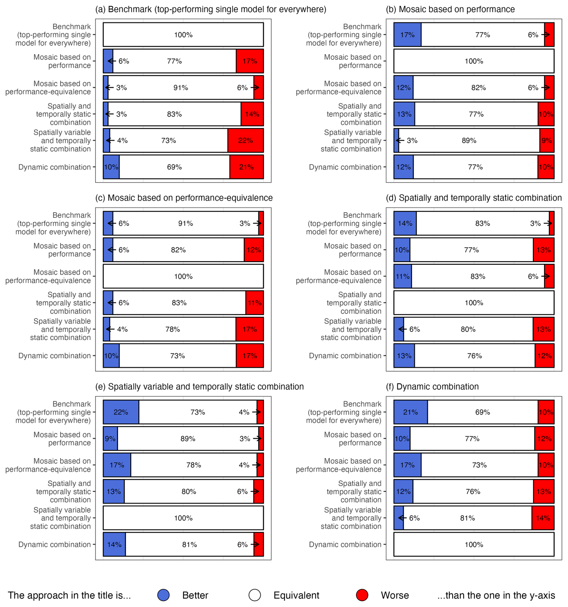
Figure 9 Bar plots comparing the equivalence between each multi-model approach against all others: (a) benchmark, (b) mosaic based on performance, (c) mosaic based on performance-equivalence, (d) spatially and temporally static combination, (e) spatially variable and temporally static combination, and (f) dynamic combination. The numbers represent the percentage of catchments falling in each category (colour) for each pairwise comparison: better (blue), equivalent (white) or worse (red).

4 Discussion

4.1 Does equivalent performance mean equivalent behaviour?

Although the different approaches tested here yield broadly similar performance scores, this does not necessarily imply that they reproduce streamflow dynamics in the same way. The composite KGE metric used for calibration and evaluation was designed to balance high- and low-flow conditions (Garcia et al., 2017), yet it remains a scalar summary of model behaviour. As such, it cannot fully capture important aspects of hydrograph dynamics – such as timing of peak flows, representation of recession limbs, or the sequencing of extreme events – which are known limitations of aggregated performance metrics (Gupta et al., 2009). Two approaches may therefore achieve comparable KGE values while differing substantially in how they represent underlying hydrological processes (e.g., Beven, 2006; Kirchner, 2006; Khatami et al., 2019; Bouaziz et al., 2021; Cinkus et al., 2023). This issue is particularly relevant for multi-model combinations, where averaging effects can mask deficiencies in individual models. Therefore, equifinality remains an important challenge: different model structures or combination schemes can lead to similar scores, but not necessarily to similar hydrological realism (e.g. Butts et al., 2004; Wagener and Gupta, 2005; Renard et al., 2010; Gupta and Govindaraju, 2019). Future analyses should therefore focus on process-oriented diagnostics to better assess to what extent “equivalent performance” implies “equivalent behaviour”. These findings also contribute to the motivation for using ensembles in a probabilistic framework, which aim to represent the range of plausible model behaviours rather than relying on a single simulation.

4.2 Can we link model structure, model performance and catchment attributes?

Establishing systematic links between model structures, their performance, and catchment attributes remains a fundamental challenge in hydrology (e.g., Knoben et al., 2020; David et al., 2022; Kiraz et al., 2023; Spieler and Schütze, 2024). However, the evidence so far suggests that these relationships are often weak or inconsistent across domains. For example, Knoben et al. (2020) showed that model performance aligns more strongly with climate and hydrological signatures than with geomorphological ones (e.g., geology, soils, vegetation). Knoben et al. also ranked the model structures according to structural similarity but found no clear relationship between model structure and catchment attributes. David et al. (2022) demonstrated that although aridity and baseflow index influence the behaviour of different structures, anticipating where a specific structure will perform well remains difficult. Kiraz et al. (2023) hence suggest selecting hydrological model structures a priori based on explicit perceptual models of the region and looking beyond statistical performance alone. This call to incorporate more process-based metrics is echoed by many other studies (e.g., Yilmaz et al., 2008; Althoff and Rodrigues, 2021; Todorović et al., 2022).

Our results point in the same direction. Across the CONUS, several single models exhibit performance comparable to the benchmark (Fig. A1) despite substantial structural differences (e.g., differences in lower architecture, baseflow computation, and percolation equations between the two top-performing models). This makes it difficult to establish clear links between model structure and performance. Although we do not conduct a dedicated analysis of catchment attributes, the spatial distribution maps of the models selected within the multi-model mosaic approaches (Figs. A2 and A4) do not reveal patterns that correspond to catchment characteristics.

In this study, we also explored multi-model combinations. Within such a modelling framework, the structure–performance–attributes relationship becomes even more complex: the goal is no longer to determine whether a single model is appropriate for a catchment, but to evaluate whether the interactions among multiple models are appropriate for that catchment. Although previous work has shown that diverse ensembles can improve streamflow simulations (e.g., Winter and Nychka, 2010; Seiller et al., 2012; Thébault et al., 2024), the direct connections between ensemble composition and catchment characteristics remain poorly constrained.

A promising avenue for addressing these challenges is the use of large-sample emulators that predict model parameters as a function of catchment characteristics (Tang et al., 2025; Farahani et al., 2025) or differentiable models that build a direct connection between catchment attributes and parameters (Feng et al., 2022; Song et al., 2024). Another research perspective is to enrich multi-model mosaic approaches with perceptual-model constraints or additional process-based diagnostics to help reduce equifinality and improve realism.

4.3 Why does the dynamic combination not outperform other multi-model approaches?

Although the dynamic combination represents the most sophisticated of the tested approaches, its performance did not surpass that of the simpler methods. Compared to more traditional multi-model approaches such as mosaics (Knoben et al., 2020; Mai et al., 2022; Spieler and Schütze, 2024; Knoben et al., 2025) or static combinations (Shamseldin et al., 1997; Georgakakos et al., 2004; Seiller et al., 2012; Thébault et al., 2024), the dynamic combination approach (Thébault et al., 2025a) was developed recently and deliberately kept simple in this initial development. Thébault et al. (2025a) highlighted possible extensions to improve performance, such as incorporating machine learning to increase flexibility at different stages of the method. Such improvements have not yet been made in this study.

There are several further potential explanations for why the dynamic combination method does not perform as well as other multi-model methods in this paper. First, the dynamic combination was optimized using the Mean Absolute Error (MAE), a criterion that tends to emphasize the higher errors more commonly found at higher flows, while our evaluation was based on a composite KGE metric aiming to target both high- and low-flow dynamics. This mismatch may limit the apparent benefits of the method. Second, and as noted by Winter and Nychka (2010), ensemble diversity is key to enhancing the performance of multi-model approaches. Although 78 conceptual models were used, they were all calibrated using only one composite criterion, resulting in limited heterogeneity in how the models target different parts of the hydrograph. This limitation is particularly relevant for the dynamic approach, which is able to select a different model at each timestep and would therefore benefit from having parameter sets trained for specific hydrological conditions.

While the development of the dynamic combination approach is still at an early stage, performance differences remain minimal here (Sect. 3.2.1), and the results on sampling uncertainty (Sect. 3.2.2) showed a lower sensitivity to the evaluation period compared to other multi-model approaches. This reduced sensitivity is expected to some extent, because the dynamic combination is the only approach whose weights can adjust over time and thus partially compensate for differences introduced by temporal sampling. In other words, the dynamic combination appears to yield simulations with more robust performance under unseen (in time) data, which is a helpful characteristic when modelling systems undergoing change. It is also worth noting that the dynamic approach uses a different rule for forming the combination than the two other approaches evaluated here. Specifically, the current implementation of the dynamic combination selects the model weights at each time step by assuming that the m models with the highest performance over the k past windows of length τ – chosen to be similar to the current hydrological conditions – will also form the best-performing combination. In practice, this means that the combination is derived directly from individual model performance rankings, rather than by evaluating all possible model combinations. While this is a reasonable heuristic, it is nevertheless not always optimal (see e.g., Ajami et al., 2006; Seiller et al., 2012). Comparing every combination of two or three models (as done for the other combination approaches) across the different neighbours at each time step could provide better results but requires much more computational resources (${}_{\mathrm{2}}^{\mathrm{78}}C+{}_{\mathrm{3}}^{\mathrm{78}}C=\mathrm{79}\mathrm{079}$ simulations evaluated instead of the current 78). Future developments could therefore explore a more consistent or adaptive selection of the number of models within the dynamic framework to ensure a fairer comparison with static approaches.

4.4 What are the implications for hydrological prediction and practice?

From an operational perspective, our results highlight a promising pathway for using a single model everywhere. Although the benchmark – i.e., a single model for everywhere – was identified from a comprehensive multi-model evaluation (selected among a large ensemble), once this best-performing structure is known, it can be applied operationally with very limited computational cost. In other words, the initial ensemble exploration represents a research investment, whereas the resulting selected model offers a pragmatic option for agencies or practitioners looking for minimal ongoing complexity. This strategy is therefore very different from usual practice, where the model is selected based on legacy choices or convenience of use (Addor and Melsen, 2019). Yet, realizing this pathway in practice requires operational support systems (e.g. staff training, backup capabilities, product-generation workflows, and input engine) that are flexible enough to accommodate alternative model structures; the absence of such infrastructure is a key reason why operational systems often default to using a single model based on legacy. However, it is important to note that all models and multi-model approaches analysed here originate from FUSE and thus share structural similarities, which may partly explain why the top-performing single model performs comparably to the multi-model approaches. Consequently, the conclusion that a single model can perform well across diverse catchments should be interpreted with caution, as it may depend on the diversity of model structures and hydroclimatic conditions considered. Expanding the analysis to include a wider range of model architectures or climate regimes would help to further test the robustness of this finding.

Starting from an ensemble of models can also be useful to further explore the structural uncertainties of different models. Following the advances highlighted by the HEPEX community (Schaake et al., 2007; Ramos et al., 2018), there is a growing shift toward probabilistic modelling frameworks. In this regard, the FUSE model ensemble offers a particularly valuable tool, enabling the exploration of a wide range of model structures while maintaining low computational costs due to its conceptual simplicity.

At the same time, the sampling uncertainty analysis underscores that combination approaches provide greater robustness by being less sensitive to the evaluation period. For operational hydrology, this robustness may be more important than marginal gains in performance, especially when forecasting floods or low flows, or generating forecasts under changing climatic conditions. Dynamic combinations, although not yet fully mature, remain particularly promising in this regard, as they explicitly allow model weights to vary through time in response to shifting hydrological conditions.

5 Conclusions

Our study aims to compare various multi-model approaches across a large sample of catchments for streamflow simulations. To this end, 544 catchments from the CAMELS dataset (Addor et al., 2017) are used, and an ensemble of 78 lumped structures is built within FUSE (Clark et al., 2008). Six different multi-model approaches – a single model selected from a larger ensemble, a mosaic based on performance, a mosaic based on performance-equivalence, a spatially and temporally static combination, a spatially variable and temporally static combination, and a dynamic combination – are tested and compared. In conclusion, our analysis highlights the following key points:

• Multi-model approaches, as tested here and commonly found in the literature, show similar distributions of performance score and associated sampling uncertainty across a large sample of catchments. Yet, differences remain in a per-catchment comparison. Indeed, multi-model approaches achieve equivalent performance for more than 70 % of the catchments, but no approach consistently outperforms the other approaches in the remaining 30 % of catchments.

• Compared to the other methods, the spatially variable and temporally static combination shows a slightly better performance score distribution, together with one of the lowest (i.e. best) sampling uncertainty distributions, leading to the highest (i.e. best) improvement/deterioration ratio among the various multi-model approaches tested. The dynamic combination approach shows the lowest sampling uncertainty across the sample of catchments, highlighting its relative robustness when applied to unseen data.

• The availability of a large structural ensemble creates scope to identify a single model that performs well across all catchments, whose performance and sampling uncertainty are comparable to those of more complex multi-model approaches.

Looking forward, several avenues for research emerge from this study. Given the strong performance of the one-size-fits-all benchmark identified in this study, a promising extension would be to test adaptive calibration strategies within a single-structure framework. For instance, the multi-calibration approach proposed by Oudin et al. (2006), which combines parameter sets optimized for contrasting flow regimes, could offer a parsimonious alternative to multi-model strategies while retaining structural simplicity. Exploring whether such regime-dependent calibration could further enhance the robustness of a single well-chosen structure across diverse hydro-climatic conditions would constitute a valuable direction for future research. While the dynamic combination approach shows no clear benefits compared to simpler multi-model strategies, it remains in its infancy; future work should explore its potential using ensembles with greater structural diversity (e.g. physically-based or machine learning models), alternative calibration strategies (e.g. various objective functions) and a larger evaluation framework (e.g. several metrics, hydrological signatures). Importantly, this study accounts for sampling uncertainty in model performance metrics, demonstrating that apparent differences in skill can often be statistically indistinguishable. This highlights that performance scores alone may be insufficient to identify or select appropriate model structures. Moreover, an important next step is to test multi-model approaches in ungauged catchments, where model choice or weights must be transferred in space; in this context, linking multi-model performance more explicitly to catchment attributes could help improve understanding when a specific model is needed and which one. In addition, given the computational burden of large ensembles, future studies should also assess the trade-offs between complexity and practicality, to determine when sophisticated multi-model schemes are justified compared to simpler benchmark strategies. Finally, evaluating the robustness of single- and multi-model approaches under non-stationary conditions – for example using dedicated frameworks such as the Robustness Assessment Test (RAT; Nicolle et al., 2021) or structured climate-sensitivity experiments (e.g., Wood et al., 2004) – remains an open challenge. This issue is particularly critical in the context of climate change, land-use shifts, or increasing hydro-climatic extremes, where model transferability becomes a central concern for operational forecasting and long-term water resource planning. In such contexts, moving beyond a deterministic paradigm based on a single prediction to a probabilistic framework using ensembles may provide a practical means to better represent parameter and structural uncertainties.

Appendix A: Further analyses on multi-model approaches

Benchmark

As a reminder, the benchmark is defined as the model that attains the highest median KGE_comp value over the calibration period and across all the catchments. Figure A1 provides an alternative representation of Fig. 3a, showing the distribution of model performance across catchments for each individual structure. Based on this criterion, model no. 126 is selected as the benchmark. Note that this structure is mixed, i.e. it does not correspond to any of the original models (VIC, PRMS, SAC-SMA, and TOPMODEL). The details of its structural configuration are provided in Table A1.

Figure A1 Boxplot of performance scores, KGE_comp, over the calibration period for each of the 78 individual FUSE structures across all catchments. The boxplots represent the 10 %, 25 %, 50 %, 75 % and 90 % quantiles. The dashed blue line highlights the optimal value of KGE_comp.

Table A1 Description of the structure selected as benchmark, structure no. 126. Here, we keep the notation as in Clark et al. (2008).

Mosaic based on performance

The mosaic based on performance selects a single model for each catchment according to the highest KGE_comp value during the calibration period. Figure A2 shows that 57 of the 78 models are selected at least once as the top-performing model for a catchment. Structure no. 126 (Table A1) is the most dominant, being selected in 13 % of the catchments (73 out of 544).

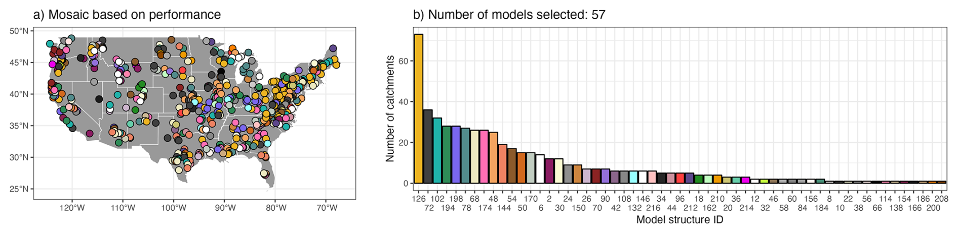
Figure A2 (a) spatial distribution of the models selected within a mosaic based on performance and (b) histogram illustrating the number of catchments where a specific model is selected, ranked by their frequency of selection.

Mosaic based on performance-equivalence

The performance-equivalence mosaic also selects a single model for each catchment. In this case, model equivalence is defined by considering both performance and the associated sampling uncertainty, resulting in multiple candidate models for a given catchment (Fig. A3). Figure A3 highlights that a large number of structures can be considered equivalent to the top-performing model in most catchments: at least 10 structures are equivalents in more than 90 % of the catchments, and the median number of equivalent structures is 28.

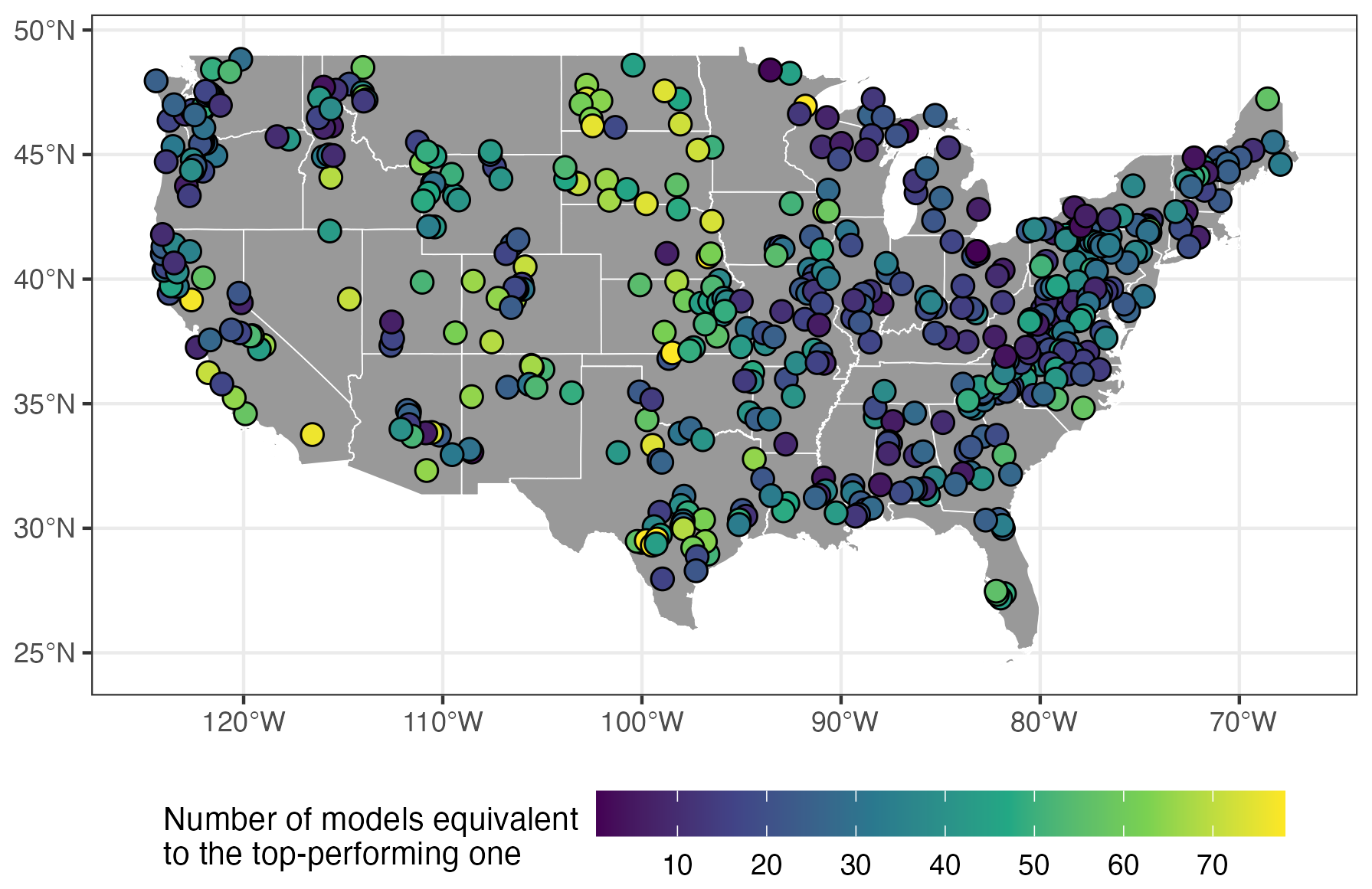
Figure A3 Spatial distribution of the number of models that are performance-equivalent to the top-performing model for each catchment.

The final model assignment is then determined by minimizing the number of distinct models used across all catchments. Figure A4 shows that only 8 of the 78 models are required to cover all the catchments. Notably, structure no. 126 (Table A1) alone accounts for 80 % of the catchments (430 out of 544). Interestingly, structure no. 72 is not used at all within this framework despite being the second top-performing single model in Fig. A1. This suggests similarities between different models. It is important to note that equivalence in this context refers solely to statistical indistinguishability with respect to KGE_comp within sampling-uncertainty bounds. Such equivalence does not imply identical hydrograph dynamics or process representations.

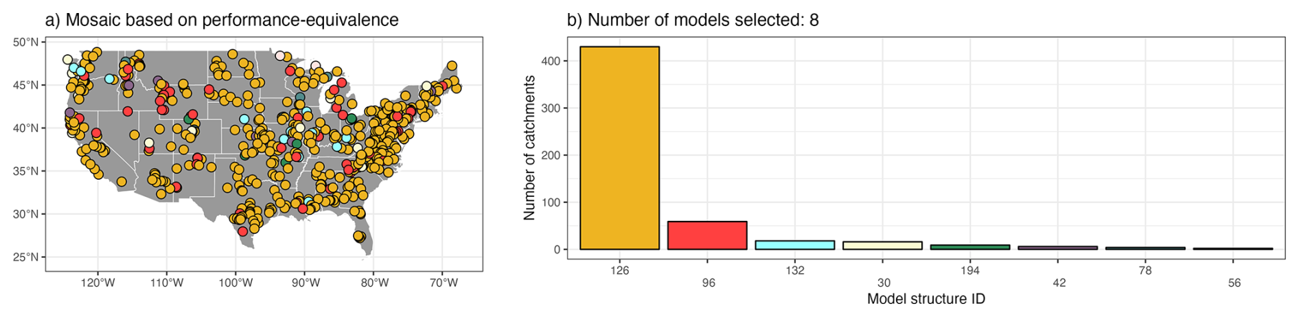
Figure A4 (a) spatial distribution of the models selected within a mosaic based on performance-equivalence and (b) histogram illustrating the number of catchments where a specific model is selected, ranked by their frequency of selection.

Spatially and temporally static combination

The spatially and temporally static combination selects a single combination of models (here, two or three models) that attains the highest median KGE_comp value over the calibration period and across all the catchments. Model combinations are computed by simple averaging, i.e., each selected model receives an equal weight. Figure A5 shows the distribution of model performance across all catchments for each possible combination. The top-performing combination is based on models no. 72 and no. 126, which are also the two top-performing models selected in the mosaic based on performance (Fig. A2). Note that although combinations of three models were permitted, the top-performing option over the entire domain consists of only two structures.

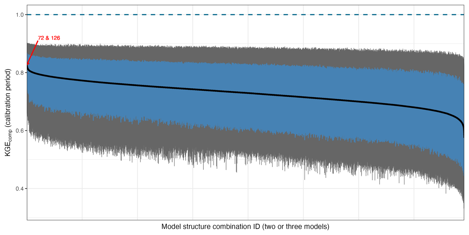
Figure A5 Distribution of performance scores, KGE_comp, over the calibration period for each of the 79 079 combinations across all catchments. The boxplots represent the 10 %, 25 %, 50 %, 75 % and 90 % quantiles. The dashed blue line highlights the optimal value of KGE_comp. The number in red highlights the top-performing combination.

Spatially variable and temporally static combination

The spatially variable and temporally static combination selects a single combination of models (here, two or three models) independently for each catchment based on performance over the calibration period. Figure A6 shows that almost every catchment required a different combination to achieve the highest performance: 439 distinct combinations are selected across the 544 catchments. Note that most of the combinations selected for more than four catchments include structure no. 126 (Table A1) and they all consist of only two structures. This result supports that testing combinations of four models was unnecessary in our case.

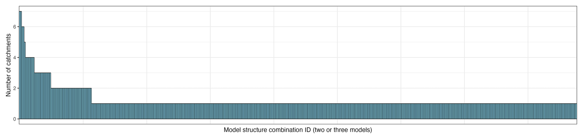
Figure A6 Histogram illustrating the number of catchments where a specific combination of models is selected, ranked by their frequency of selection, for the spatially variable and temporally static combination approach.

This analysis can be extended to the model level, i.e. identify which individual models are most frequently selected within the combinations. Figure A7 shows that all 78 structures are used at least once in a top-performing combination. In addition, structure no. 126 stands out once again, being selected in the top-performing combinations for 27 % of the catchments (148 out of 544), with structure 72 being a distant (and barely) second.

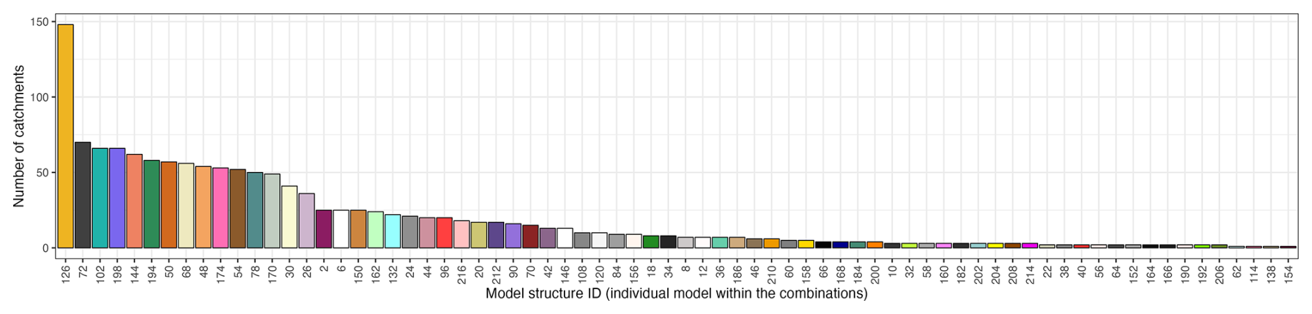
Figure A7 Histogram illustrating the number of catchments where a specific model is selected (within the combinations), ranked by their frequency of selection, for the spatially variable and temporally static combination approach.

Dynamic combination

The dynamic combination adapts the models included in the combination across both space and time based on similarities in past hydrological conditions. This method requires three parameters: the length of the time window (τ, ranging from 4 to 28 d), the number of nearest neighbours (k, ranging from 1 to 19), and the number of models to combine (m, ranging from 1 to 19). Figure A8 provides the distribution of these parameters across catchments. The parameter controlling the length of the time window (τ) reveals a clear divide between catchments that require short periods and those that require long periods to characterize current conditions and similar past windows. This difference likely reflects differences between catchments dominated by fast, event-driven dynamics and those governed by slower, longer-term processes. The distribution of the number of models to be combined is strongly skewed toward low values, with m £5 in nearly 70 % of the catchments.

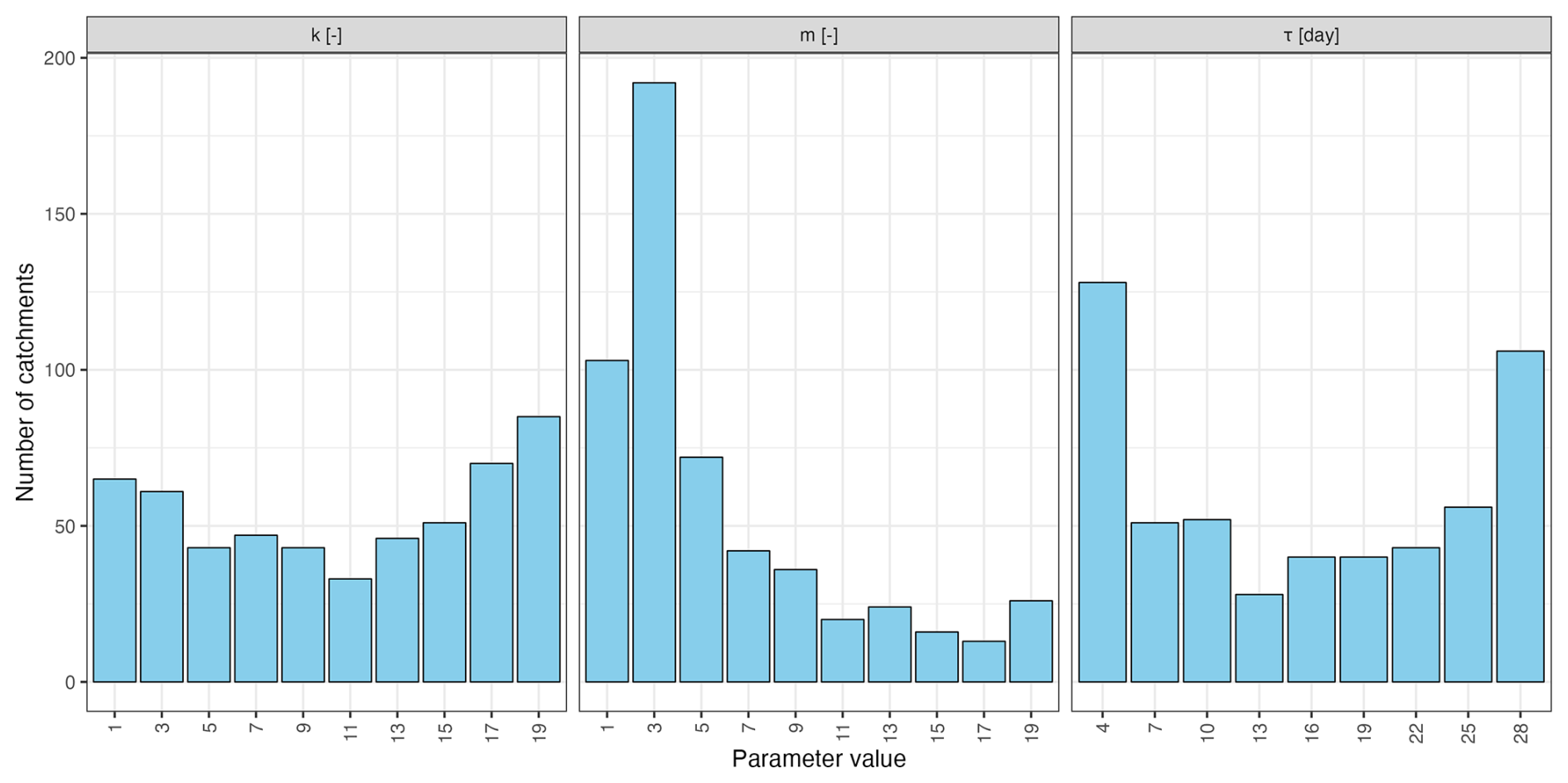
Figure A8 Distribution of the dynamic combination parameters (k, m and τ) across all the catchments.

Because the combinations vary over time and may include up to 19 different models, analysing the individual combinations is impractical. However, an analysis at the structure level – i.e. examining how often each individual model is included in the combinations – remains feasible. Figure A9 shows the percentage of use (both temporal and spatial) for each structure. All 78 structures are used at least once in at least one catchment. In contrast to the results from the previous multi-model approaches, structure no. 126 does not stand out markedly from the others. The small range in usage percentages (from 0.5 % to 2.8 %) indicates that all models are used relatively frequently in the dynamic combination, suggesting that temporal dynamics must play a key role in model selection.

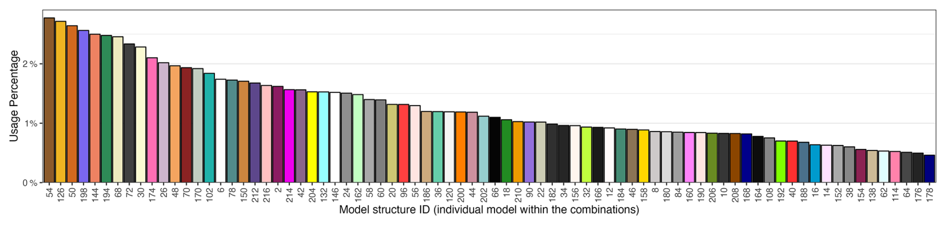
Figure A9 Histogram illustrating the number of catchments where a specific model is selected (within the combinations), ranked by their frequency of selection, for the dynamic combination approach.

This analysis can be further refined to examine the temporal dynamics of model selection at the scale of each catchment. Figure A10 shows the percentage of use (through time) of each structure (within the combinations) for every catchment. Notably, several vertical bands of lighter colours indicate specific models that are frequently selected across many catchments. Conversely, some horizontal lines exhibit gaps, showing that only a limited subset of models is selected for those specific catchments. It is worth noting that a temporal-scale analysis would also be possible. However, given the catchment-specific dynamics, it is difficult to identify general trends without first grouping the catchments into clusters.

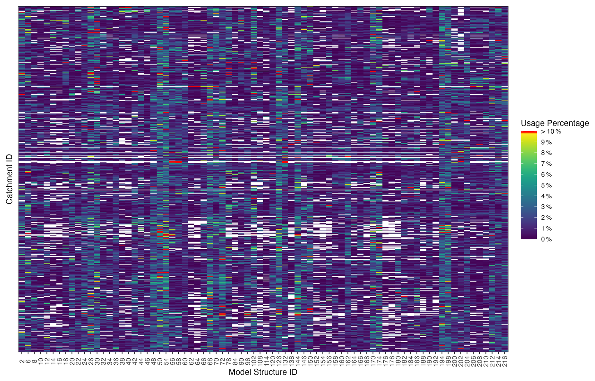
Figure A10 Percentage of use of each model structure within the dynamic combinations for every catchment. Each row corresponds to a catchment and each column to a model structure. Colours indicate the proportion of time steps in which a given structure is included in the optimal combination for that catchment. White colour indicates 0 %. Catchments are ordered according to their gauged station identifiers; it does not reflect performance or catchment attributes, although station numbering broadly follows a regional logic.

Appendix B: Individual models and sampling uncertainty failures

Among the initial 559 catchments, 15 were removed due to model failures or because sampling uncertainties could not be computed. Figure B1 shows the location of the catchments experiencing such failures for each approach. The following bullet points explain the failure for each catchment (USGS gauge ID):

Figure B1 Spatial distribution of the catchments that were excluded due to a failure during model calibration or sampling uncertainty calculation for each multi-model approach.

• 02427250: Failed on the mosaic based on performance-equivalence due to a criterion in the sampling-uncertainty calculation: only nine years contained more than 100 valid days over the calculation period (here the calibration), whereas ten years are required.

• 04056500: All approaches failed because no model calibrated successfully for this catchment. The snow module failed due to a negative area for elevation band 2 in the CAMELS file.

• 05062500: Failed on the mosaic based on performance-equivalence due to a criterion in the sampling-uncertainty calculation: only nine years contained more than 100 valid days over the calculation period (here the calibration), whereas ten years are required.

• 05412500: Failed on the benchmark and the spatially and temporally static combination because both structure no. 72 and no. 126 did not calibrate successfully. Notably, 71 out of 78 structures did not calibrate due to a negative area for elevation band 3 in the CAMELS file.

• 06354000: Failed on the spatially and temporally static combination because structure no. 72 did not calibrate successfully. Notably, 56 out of 78 structures did not calibrate due to a negative area for elevation bands 2 & 4 in the CAMELS file.

• 06360500: Failed on the spatially and temporally static combination because structure no. 72 did not calibrate successfully. Notably, 66 out of 78 structures did not calibrate due to a negative area for elevation bands 3, 4 & 5 in the CAMELS file.

• 06441500: Failed on the spatially and temporally static combination because structure no. 72 did not calibrate successfully. Notably, 64 out of 78 structures did not calibrate due to a negative area for elevation bands 3 & 4 in the CAMELS file.

• 06447000: Failed on the spatially and temporally static combination because structure no. 72 did not calibrate successfully. Notably, 59 out of 78 structures did not calibrate due to a negative area for elevation bands 3, 4 & 5 in the CAMELS file.

• 06452000: Failed on the spatially and temporally static combination because structure no. 72 did not calibrate successfully. Notably, 64 out of 78 structures did not calibrate due to a negative area for elevation bands 2, 3, 4, 5 & 7 in the CAMELS file.

• 06468250: Failed on the spatially and temporally static combination because structure no. 72 did not calibrate successfully. Notably, 64 out of 78 structures did not calibrate due to a negative area for elevation band 1 in the CAMELS file.

• 07263295: Failed on the mosaic based on performance-equivalence due to a criterion in the sampling-uncertainty calculation: only nine years contained more than 100 valid days over the calculation period (here the calibration), whereas ten years are required.

• 07362587: Failed on the mosaic based on performance-equivalence due to a criterion in the sampling-uncertainty calculation: only nine years contained more than 100 valid days over the calculation period (here the calibration), whereas ten years are required.

• 09484600: Failed on the mosaic based on performance-equivalence due to a criterion in the sampling-uncertainty calculation: only nine years contained more than 100 valid days over the calculation period (here the calibration), whereas ten years are required.

• 11151300: Failed on the benchmark and the spatially and temporally static combination because structure no. 126 did not calibrate successfully.

• 12141300: Failed on the mosaic based on performance-equivalence due to a criterion in the sampling-uncertainty calculation: only nine years contained more than 100 valid days over the calculation period (here the calibration), whereas ten years are required.

Appendix C: Comparison between single-model and multi-model combinations

In the multi-model combination framework presented in Sect. 2.5.3, combinations were restricted to sets of two or three models. Single-model combinations (i.e., combinations of size one) were not included in the search space. This choice was made to explicitly distinguish combinations from mosaics. To assess the potential impact of this restriction, we compared, for each catchment, the top-performing single model (i.e. mosaic based on performance) with the top-performing two- or three-model combination (i.e. spatially variable and temporally static combination) over the calibration period.

Figure C1 shows that across all catchments, the top-performing single model achieved a higher KGE_comp score than any two- or three-model combination in 73 catchments (13 % of the sample). In the remaining 471 catchments, the top-performing multi-model combination outperformed the single structure. This indicates that although model combinations tend to improve performance overall, they do not systematically outperform individual models in every catchment. Figure C1 also highlights that performance difference between the top-performing single model and the top-performing multi-model combination remain small, suggesting that the exclusion of size-one combinations has a limited influence on the overall performance distributions reported in the main manuscript. Allowing combinations of size one would lead to minor improvements in a limited subset of catchments but would not alter the overall ranking of modelling approaches or the main conclusions of this study.

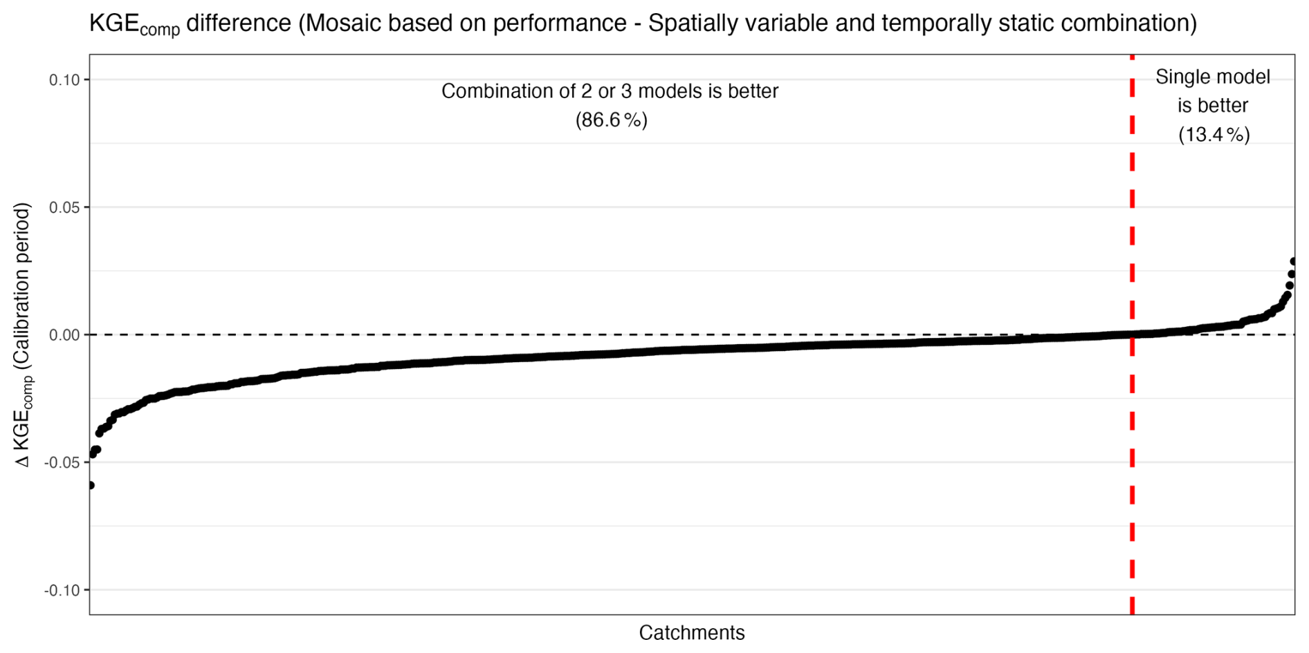
Figure C1 Difference of performance KGE_comp between the top-performing single model and the top-performing combination (two or three models) for each catchment over the calibration period. Each dot represents a catchment, and they are ordered by difference of performance. The dashed black line indicates equality; dots under show that the top-performing combination is better than the top-performing single model and vice versa. The dashed red line highlights the tipping point.

Appendix D: Spatial pattern of equivalence between multi-model approaches

Figure D1 shows the spatial distribution of the equivalence analysis between each multi-model approach. The spatial organization indicates that multi-model approaches – particularly the combination-based methods – tend to improve performance in catchments that already exhibit relatively high KGE_comp values and comparatively low sampling uncertainty. In contrast, deteriorations relative to the benchmark are primarily observed in catchments with lower performance and larger uncertainty.

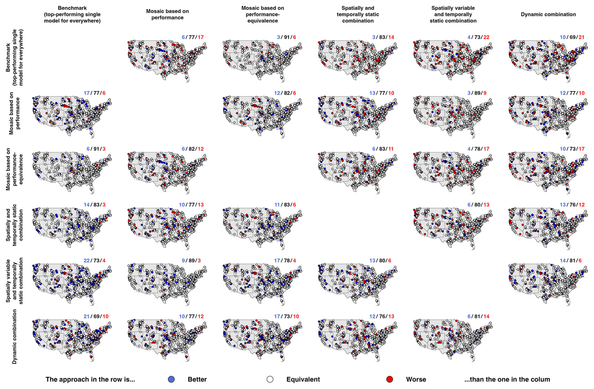
Figure D1 Maps comparing the equivalence between the multi-model approaches. The numbers (e.g. 0/100/0) represent the percentage of catchments falling in each category (colour): better (blue numbers and dots), equivalent (black numbers, white dots) or worse (red numbers and dots).

This pattern may reflect the greater difficulty of improving simulations in catchments where dominant hydrological processes are either weakly represented or structurally absent in the model ensemble (e.g., prairie pothole regions or highly arid areas). In such cases, calibration may lead to overfitting during the calibration period without improving generalization.