Assessing national exposure to and impact of glacial lake outburst floods considering uncertainty under data sparsity

Glacial lake outburst floods (GLOFs) are widely recognised as one of the most devastating natural hazards in the Himalayas, with catastrophic consequences, including substantial loss of life. To effectively mitigate these risks and enhance regional resilience, it is imperative to conduct an objective and holistic assessment of GLOF hazards and their potential impacts over a large spatial scale. However, this is challenged by the limited availability of data and the inaccessibility to most of the glacial lakes in high-altitude areas. The data challenge is exacerbated when dealing with multiple lakes across an expansive spatial area. This study aims to exploit remote sensing techniques, well-established Bayesian regression models for estimating glacial lake conditions, cutting-edge flood modelling technology, and open data from various sources to innovate a framework for assessing the national exposure and impact of GLOFs. In the innovative framework, multi-temporal imagery is utilised with a random forest model to extract glacial lake water surfaces. Bayesian models are employed to estimate a plausible range of glacial lake water volumes and the associated GLOF peak discharges while accounting for the uncertainty stemming from the limited sizes of the available data and outliers within the data. A significant number of GLOF scenarios is subsequently generated based on this estimated plausible range of peak discharges. A graphics processing unit (GPU)-based hydrodynamic model is then adopted to simulate the resulting flood hydrodynamics in different GLOF scenarios. Necessary socio-economic information is collected and processed from multiple sources, including OpenStreetMap, Google Earth, local archives, and global data products, to support exposure analysis. Established depth–damage curves are used to assess the GLOF damage extents for different exposures. The evaluation framework is applied to 21 glacial lakes identified as potentially dangerous in the Nepalese Himalayas. The results indicate that, in the scenario of a complete breach of dam height across 21 lakes, Tsho Rolpa Lake, Thulagi Lake, and Lower Barun Lake bear the most serious impacts of GLOFs on buildings, roads, and agricultural areas, while Thulagi Lake could influence existing hydropower facilities. One unnamed lake in the Trishuli River basin, two unnamed lakes in the Tamor River basin, and three unnamed lakes in the Dudh River basin have the potential to impact more than 200 buildings. Moreover, the unnamed lake in the Trishuli River basin has the potential to inundate existing hydropower facilities.

1 Introduction

Glacial lake outburst floods (GLOFs) are recognised as one of the most impactful natural hazards in the Himalayas, where these disasters have had the highest death toll worldwide and caused serious economic damage (Veh et al., 2020). GLOFs can generate transient discharges that are orders of magnitude greater than the typical annual floods in the receiving rivers (Cenderelli and Wohl, 2001), and some of them can travel >200 km downstream (Richardson and Reynolds, 2000). The extreme discharges, accelerating along the steep mountainous terrains, make GLOFs extremely destructive to downstream communities and infrastructure systems. The unpredictable nature of GLOFs, often occurring without warning, has left downstream communities and infrastructures ill-prepared, causing the loss of human lives and economic damages. The ongoing impact of climate change has introduced additional uncertainty into GLOF risk. The Himalayan region is observing extensive glacier shrinkage and a proliferation of glacial lakes (Zhang et al., 2015). The potential impacts of GLOFs on downstream communities are expected to intensify further due to population growth and socio-economic development. Hence, it is crucial to develop effective strategies for managing GLOF risks to enhance human safety and support sustainable development. This necessitates the requirement of reproducible assessment of GLOF hazards and their potential impacts arising from these glacial lakes.

Some potentially dangerous lakes have been well-studied individually, such as Tsho Rolpa Lake (e.g. Shrestha and Nakagawa, 2014), Imja Tsho Lake (e.g. Somos-Valenzuela et al., 2015), and Lower Barun Lake (e.g. Sattar et al., 2021). However, these studies provide limited insight into the overall danger and potential impacts of glacial lakes as a whole. While there have been assessments of glacial lake hazards in the Himalayan region, certain limitations exist. Previous work by Mool et al. (2011) and Bajracharya et al. (2020) employed remote sensing techniques to identify potentially dangerous glacial lakes (PDGLs) in Nepal, considering different hazard factors. Rounce et al. (2017) undertook a similar study, quantifying the hazard levels of 131 glacial lakes with areas >0.1 km² in Nepal. Furthermore, Rounce et al. (2017) evaluated the potential downstream impacts of GLOFs caused by these glacial lakes using a simple flood model without any physical basis. This simple flood model has also been applied to evaluate the overall impacts of GLOFs originating from multiple glacial lakes in the Indian Himalayas (Dubey and Goyal, 2020). Zheng et al. (2021) extended their analysis to assess the impacts of GLOFs across the Third Pole by using a Geographic Information System (GIS)-based hydrological model. However, the complexity of GLOFs renders simple flood models inadequate for capturing their dynamics, thereby making them incapable of supporting detailed assessments of potential impacts on downstream communities and infrastructure.

A range of physically based hydrodynamic models have been developed and applied to predict the spatial–temporal processes of GLOFs, offering detailed insights into the resulting flood impacts (e.g. Worni et al., 2012; Ancey et al., 2019; Sattar et al., 2019). Recently, researchers explored the use of a hydrodynamic model to assess GLOF downstream impacts at the Third Pole (Zhang et al., 2023b). However, hydrodynamic models entail a huge amount of computation and face substantial demands for computation resources when applied at a large scale. What is even more challenging is that the computational requirements increase significantly when addressing GLOF simulations involving a large number of scenarios, which is necessary for assessing GLOFs' potential impact due to the complexity and uncertainty of the glacier lake breach process. Moreover, the application of hydrodynamic models to support GLOF modelling and impact assessment necessitates a considerable amount of data, and data availability poses another significant challenge.

The high-alpine conditions have constrained our ability to acquire detailed spatial data for multiple lakes across a large scale. To correctly depict the dynamic inundation process of GLOFs, glacial lake conditions and dam breach processes are essential for estimating the outflow discharge resulting from a breach. While the distribution and changes of glacial lakes have been mapped extensively from increasingly available satellite imagery (e.g. Zhang et al., 2015; Nie et al., 2017; Shugar et al., 2020), accurately determining lake volumes and reliably predicting dam breach processes has remained a challenge because high-alpine conditions impede detailed fieldwork. Combining satellite imagery with existing lake bathymetry measurements offers the possibility of estimating water volumes and peak discharges from outbursts by establishing empirical relationships (e.g. Zhang et al., 2023a). However, estimated lake volumes and potential peak discharges derived from these empirical relationships can vary by up to 1 order of magnitude (Cook and Quincey, 2015; Muñoz et al., 2020). To account for the uncertainties inherent in conventional empirical relationships, Veh et al. (2020) developed a Bayesian robust regression, utilising data from the bathymetric survey of 24 glacial lakes. This model estimates water volume based on the surface areas of glacial lakes. Simultaneously, they created a Bayesian variant of a physical dam breach model originally proposed by Walder and O'Connor (1997) to predict the peak discharge associated with the flood volume. The Bayesian estimates explore the parameter space of plausible flood volumes and the associated peak discharges, generating 1 million possible outburst scenarios for each lake. These scenarios comprehensively consider all potential conditions of the dam breach process for each specific lake and provide a full range of input information for hydrodynamic models, thereby facilitating predictions of the GLOF inundation process. Therefore, this study aims to leverage these established Bayesian models to support GLOF inundation simulations.

GLOF exposure and impact assessment are also restricted by data sparsity. Previous studies have typically relied on census data at coarse spatial resolutions or aggregated land use data that encompass various objects like properties and infrastructure to estimate the potential socio-economic impact of GLOFs (e.g. Shrestha and Nakagawa, 2014; Rounce et al., 2016). Benefiting from the emergence of new data technologies and the resulting enhancements in data quantity and quality, a spatially explicit assessment method has been developed to identify GLOF exposure at an object level and has been applied to Tsho Rolpa Lake (Chen et al., 2022). Employing a similar strategy, essential socio-economic information is collected and processed from various sources, including OpenStreetMap (OSM), Google Earth, global data products, and local archives. The information is used to create a spatial exposure dataset that specifies the locations of different objects, such as individual buildings and hydropower facilities. Subsequently, these spatial exposure data are overlaid with the spatially distributed flood simulation outputs to identify potential exposure to GLOFs along their path.

Overall, this study aims to create a framework for object-based exposure and potential impact assessments of GLOFs for multiple lakes at a large scale by integrating remote sensing techniques, the developed Bayesian regression models for estimating lake volumes and potential peak discharges, a physically based hydrodynamic model supported by parallelised high-performance computing, and socio-economic information from multiple sources. Nepal has been chosen as the test area due to its abundance of glacial lakes, and it has been reported to experience the most significant national-level economic consequences from GLOFs globally (Carrivick and Tweed, 2016).

2 Methodology and data

The proposed framework for object-based exposure and impact assessment of GLOFs across multiple lakes comprises several key components: extraction of glacial lake water surfaces from multi-temporal imagery, estimation of lake volumes and peak discharges using well-established Bayesian regression models, utilization of a high-performance hydrodynamic flood model accelerated by graphics processing unit (GPU) technology, and creation of an exposure dataset from open-source data (Fig. 1). In particular, leveraging multi-temporal imagery availability, a random forest model is developed using a set of predictor variables to delineate the maximum extent of glacial lake water surfaces. The plausible range of glacial lake water depths, volumes, and GLOF-induced peak discharges is estimated through existing Bayesian models. A substantial number of GLOF scenarios, encompassing outflow discharge hydrographs through glacial lakes, is sampled based on the plausible range of peak discharges. For each scenario, the resulting outflow discharge hydrograph is employed to drive the GPU-accelerated hydrodynamic model, efficiently simulating the temporal and spatial dynamics of floods. These flood dynamics are then overlaid with the spatial exposure data to identify potential exposure to GLOFs and quantify damage extent by using established depth–damage curves.

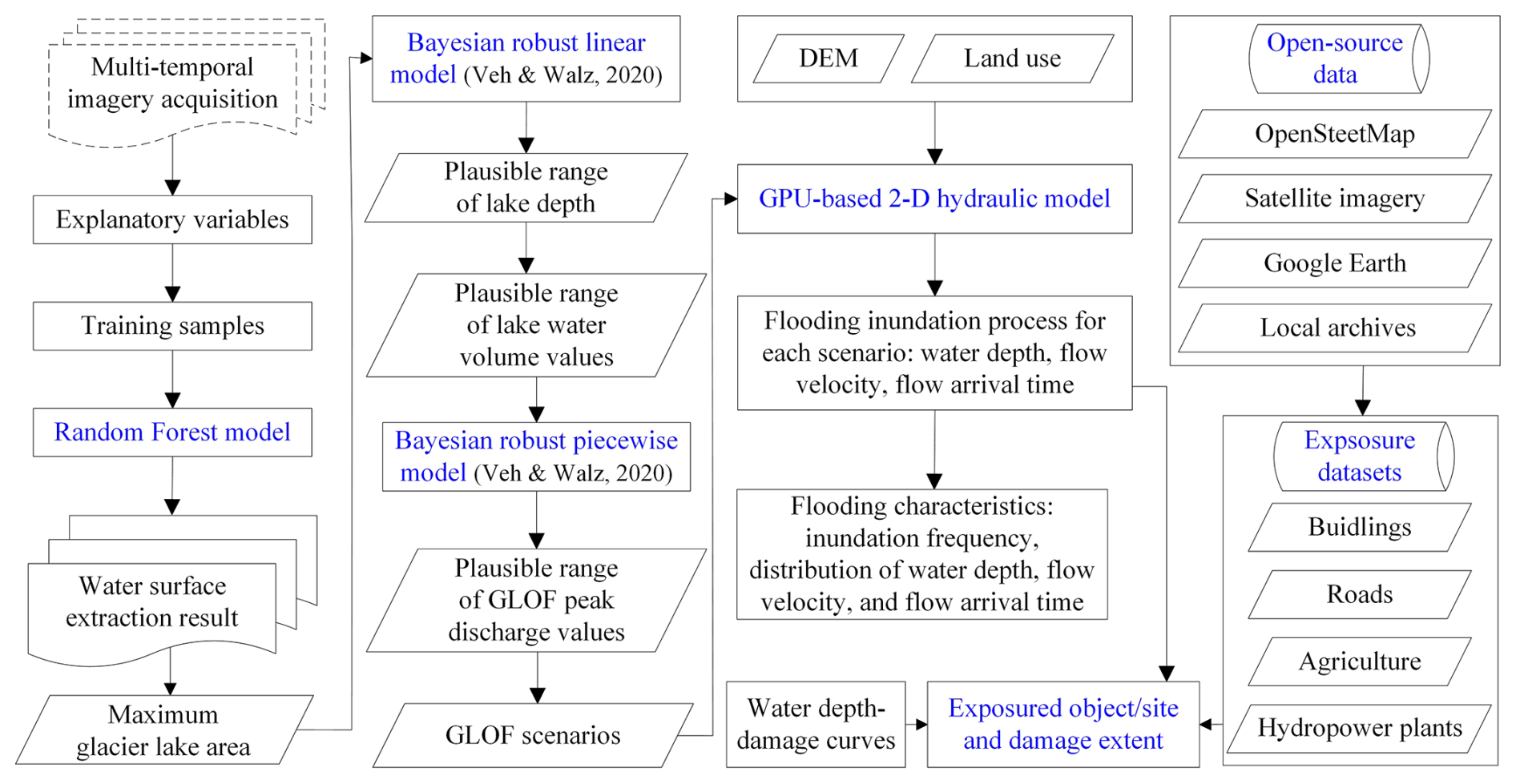
Figure 1 GLOF exposure and impact assessment framework for multiple glacial lakes (key components highlighted in blue).

2.1 Glacial lake water surface extraction

With the availability of multi-temporal imagery, a random forest model based on a set of predictor variables is used to map the location and extent of water surfaces of glacial lakes under different hydrological conditions to produce the maximum extent of lake water surfaces.

2.1.1 Acquisition of satellite imagery

Sentinel-2 is an operational multi-spectral imaging mission of the European Space Agency for global land observation. The Sentinel-2A and Sentinel-2B satellites were launched in 2015 and 2017, respectively. These satellites capture imagery every 10 d (every 5 d with the twin satellites together). The spatial resolution for the visible and broad near-infrared (NIR) bands is 10 m, while it is 20 m for the red edge, narrow NIR, and short-wave infrared bands. Here, all available Sentinel-2 imagery for the case study of glacial lakes is utilised to identify the maximum extent of their water surfaces. The analysis is based on the Sentinel-2 level-1C top-of-atmosphere (TOA) products, which are accessible through Google Earth Engine. Any observations affected by clouds are masked using the Sentinel-2 quality-assurance band flags. Bands originally at 20 m resolution are resampled to 10 m using the nearest-neighbour method before being stacked for subsequent interpretation. All available Sentinel-2 datasets are collected and filtered to preserve imagery from the ablation season, reducing the impact of frozen water surfaces as per the empirical period of the local melt season (Shugar et al., 2020). In total, 1520 Sentinel-2 images have been collected for this purpose.

2.1.2 Random forest model

Mapping water surfaces from multiple images is a complex task that necessitates the consideration and analysis of various water-related signals in spectral responses, which is often influenced by water turbidity and bottom sediments. In this context, a random forest model is developed based on a set of predictor variables to extract water surfaces. Random forest modelling is an ensemble classification technique (Breiman, 2001) and has been used extensively in the classification of remote sensing data (e.g. Yu et al., 2011; Rodriguez-Galiano et al., 2012). Random forest models excel at recognising regional variations in threshold values, surpassing the capabilities of traditional index-thresholding methods (Tulbure et al., 2016). Notably, random forest models do not rely on data distribution assumptions and can yield accurate predictions without overfitting data. Consequently, they have been used increasingly in water surface extraction as a favourable alternative to traditional statistical approaches (e.g. Schaffer-Smith et al., 2017).

A random forest model consists of a set of classification trees, each of which grows from a random subset of training samples and randomly permuted explanatory variables. The classification trees can grow to a specified maximum number without pruning, and the final classifications are determined by the majority votes of the trees in the forest. The explanatory variables for Sentinel-2 datasets in the random forest model include TOA reflectance for every spectral band, brightness temperature, vegetation indices, and water indices. TOA reflectance and brightness temperature are obtained by normalising the target imagery, mitigating unwanted effects resulting from variations in the Sun angle and Earth–Sun distance. The vegetation indices include the Normalized Difference Vegetation Index (NDVI) and the Enhanced Vegetation Index (EVI). The NDVI is sensitive to chlorophyll and is used to assess terrestrial vegetation conditions (Tucker, 1979), while the EVI is developed to optimise the vegetation signal in high biomass regions, decouple the canopy background signal, and reduce atmospheric influences (Huete et al., 2002). Water indices include the Normalized Difference Water Index (NDWI; McFeeters, 1996), Modified NDWI (MNDWI; Xu, 2006), and Normalized Difference Moisture Index (NDMI; Gao, 1996). The NDWI enhances the response to open-water features while minimising soil and terrestrial vegetation influences. The MNDWI substitutes the middle-infrared band for the NIR band used in the NDWI to enhance water features and remove noise from other land types. The NDMI is an effective indicator of vegetation water content. The training samples are selected via visual interpretation of satellite images to represent glacial lake water surfaces along with various non-water covers, including diverse landscapes and vegetation types. The uncertainty in estimating the glacial lake area is quantified using a widely used buffer method (Granshaw and Fountain, 2006). A buffer area of half a pixel (e.g. Zhang et al., 2015; Krause et al., 2019) is adopted to measure the uncertainty in the estimated lake area. The misclassified glacial lake water areas resulting from terrain shadows are eliminated during post-processing through manual exclusion of inaccurately classified regions.

2.2 GLOF dynamic inundation process simulation

Using the maximum extent of glacial lake water surfaces, we employ the established Bayesian models to predict glacial lake conditions and the dam breach process. This allows us to estimate the full range of GLOF outflow discharge through the breach. Subsequently, various GLOF scenarios featuring a range of outflow discharge hydrographs are sampled to drive the GPU-based hydrodynamic model for the simulation of flood dynamics resulting from GLOFs.

2.2.1 Estimating volumes and peak discharges of glacial lakes

Global samples from glacial lakes have suggested that the water depths for glacial lakes with similar surface areas can vary by 1 order of magnitude. To estimate the water volumes of glacial lakes, we adopted the model that relates lake areas to their maximum depths, which was developed by Veh et al. (2020). The model was built by compiling the reported lake areas and maximum depths obtained from bathymetric surveys conducted on 24 Himalayan glacial lakes. A Bayesian robust linear regression with a normally distributed target variable (lake depth d) $d\sim N\left({\mathit{\mu }}_d\right(a),\mathrm{1}/\mathit{\tau })$ is adopted to account for possible effects of the limited sample size and outliers present in the compiled dataset. The mean μ_d(a) is calculated below through a linear combination of the input lake area a. The precision τ (the inverse of variance) is the gamma-distributed $\mathit{\tau }\sim \mathrm{\Gamma }(\mathrm{0.001},\mathrm{0.001})$.

$$\begin{array}{}\text{(1)}& {\mathit{\mu }}_d\left(a\right)={\mathit{\alpha }}_{\mathrm{0}}+{\mathit{\alpha }}_{\mathrm{1}}a\end{array}$$

a is the lake area, ${\mathit{\alpha }}_{\mathrm{0}}\sim N(\mathrm{0},{\mathrm{10}}^{-\mathrm{12}})$ is the intercept, and ${\mathit{\alpha }}_{\mathrm{1}}\sim N(\mathrm{0},{\mathrm{10}}^{-\mathrm{12}})$ is the slope.

We obtained 100 posterior estimates for d from the Bayesian model for each lake. For each lake, samples inside the 95 % highest density interval (HDI) of credible lake depth values are reserved, i.e. 94 lake depth samples for each lake. In this study, we maintained the same assumption regarding the bathymetry of the glacial lakes as outlined by Veh and Walz (2020). The delineated lake from satellite imagery is circular, and each lake is assumed to have an ellipsoidal bathymetry. Therefore, we obtained 94 estimates of the total volume (V_tot) for each glacial lake.

$$\begin{array}{}\text{(2)}& V_{\text{tot}}=(\mathrm{2}/\mathrm{3})da\end{array}$$

With regard to estimating peak discharge during dam failure, Veh and Walz (2020) built a Bayesian piecewise robust model to characterise the physically motivated model developed by Walder and O'Connor (1997). The latter model predicts peak discharge Q_p during natural dam failure. In their study, Walder and O'Connor (1997) compiled data from 63 observed natural dam breaks in various settings and identified a constant response of dimensionless peak discharge $Q_{\mathrm{p}}^{*}$ when plotted against the dimensionless product η of lake volume and breach rate k. They inferred a model that describes the relationship between peak discharge and lake volume using the dimensionless peak discharge $Q_{\mathrm{p}}^{*}$.

$$\begin{array}{}\text{(3)}& {\displaystyle }{Q}_{\mathrm{p}}^{*}=Q_{\mathrm{P}}{g}^{-\frac{\mathrm{1}}{\mathrm{2}}}{h}^{-\frac{\mathrm{5}}{\mathrm{2}}}\text{(4)}& {\displaystyle }\mathit{\eta }=V_O^{*}{k}^{*}\end{array}$$

$V_O^{*}=V_{\mathrm{0}}{h}^{-\mathrm{3}}$ represents the dimensionless flood volume, $k^{*}=k{g}^{-\mathrm{1}/\mathrm{2}}{h}^{-\mathrm{1}/\mathrm{2}}$ is the dimensionless breach rate, g is the acceleration of gravity, h is the breach depth, and V₀ is the released water volume (flood volume). k is the breach rate and subsumes lithological conditions, the erodibility of the outflow channel, and the breach and downstream valley geometry. h is measured from the final lake surface after dam failure to the initial lake surface. V₀ is the released water volume and depends on h and V_tot.

Empirical data support a piecewise regression model in the form $Q_{\mathrm{p}}^{*}=b_{\mathrm{0}}{\mathit{\eta }}^{b_{\mathrm{1}}}$ (b₀ and b₁ are the regression parameters) for η<η_c, and $Q_{\mathrm{p}}^{*}$ is constant for η>η_c. Bayesian piecewise linear regression was developed to predict peak discharge $Q_{\mathrm{p}}^{*}$ from η, which is the product of the breach rate k and the released flood volume (Veh and Walz, 2020). The extent of breaching is closely linked to the geometry and material composition of the dam. To account for the theoretically most severe GLOFs, the maximum breach depth is considered to reach the marine dam's maximum height and extend from the dam crest down to the point where the hummocky terrain ends, as determined using high-resolution satellite imagery and DEM data. The dam maximum height data were requested from and obtained through Bajracharya et al. (2020) and are presented in Table 1. For each lake, we predicted peak discharge Q_p based on given values of V_tot and η using the Bayesian piecewise linear regression model. We generated 100 estimates of the posterior predicted Q_p for each given value of V_tot and η. The values of η for individual lakes encompass the assumed flood volumes, and we also considered 100 physically plausible values of the breach rate k based on a log-normal fit to reported breach rates. By multiplying the 94 samples of V_tot by the 100 samples of k and 100 samples of Q_p, we ultimately obtained a total of 940 000 scenarios of Q_p per lake. Considering the substantial computational resources required for GLOF inundation simulations in Sect. 2.2.2, 100 scenarios are selected from the 940 000 Q_p and associated V₀ scenarios per lake using k-means clustering. The k-means algorithm partitions the Q_p and V₀ data into 100 clusters, optimising intra-cluster homogeneity and inter-cluster heterogeneity. By selecting the data point closest to the centroid of each cluster, the selected scenarios ensure diverse and representative sampling across the full spectrum of the dataset. The weight of each selected scenario is determined by its occurrence probability, specifically the proportion of times its peak discharge does not exceed that of other scenarios relative to the total number of scenarios. A smaller proportion indicates a lower likelihood of occurrence, while a larger proportion indicates a higher likelihood. The weight of each scenario is calculated by dividing the proportion by the total proportion of all possible scenarios. In these simulations, the dam breach hydrograph is assumed to have an isosceles triangle shape, simplifying its derivation from Q_p and V₀. The breach hydrograph then serves as the boundary condition for the hydrodynamic modelling. Although there is some uncertainty, the assumption of an isosceles triangle shape for the dam breach hydrograph aligns with experimental observations (e.g. Morris et al., 2007; Walder et al., 2015; Yang et al., 2015) and is supported by simulation results from commonly used mechanisms and empirical models (e.g. Yang et al., 2023). Apart from the theoretically most severe scenarios, less severe conditions are also considered, where 10 %, 30 %, and 50 % of dam heights are breached.

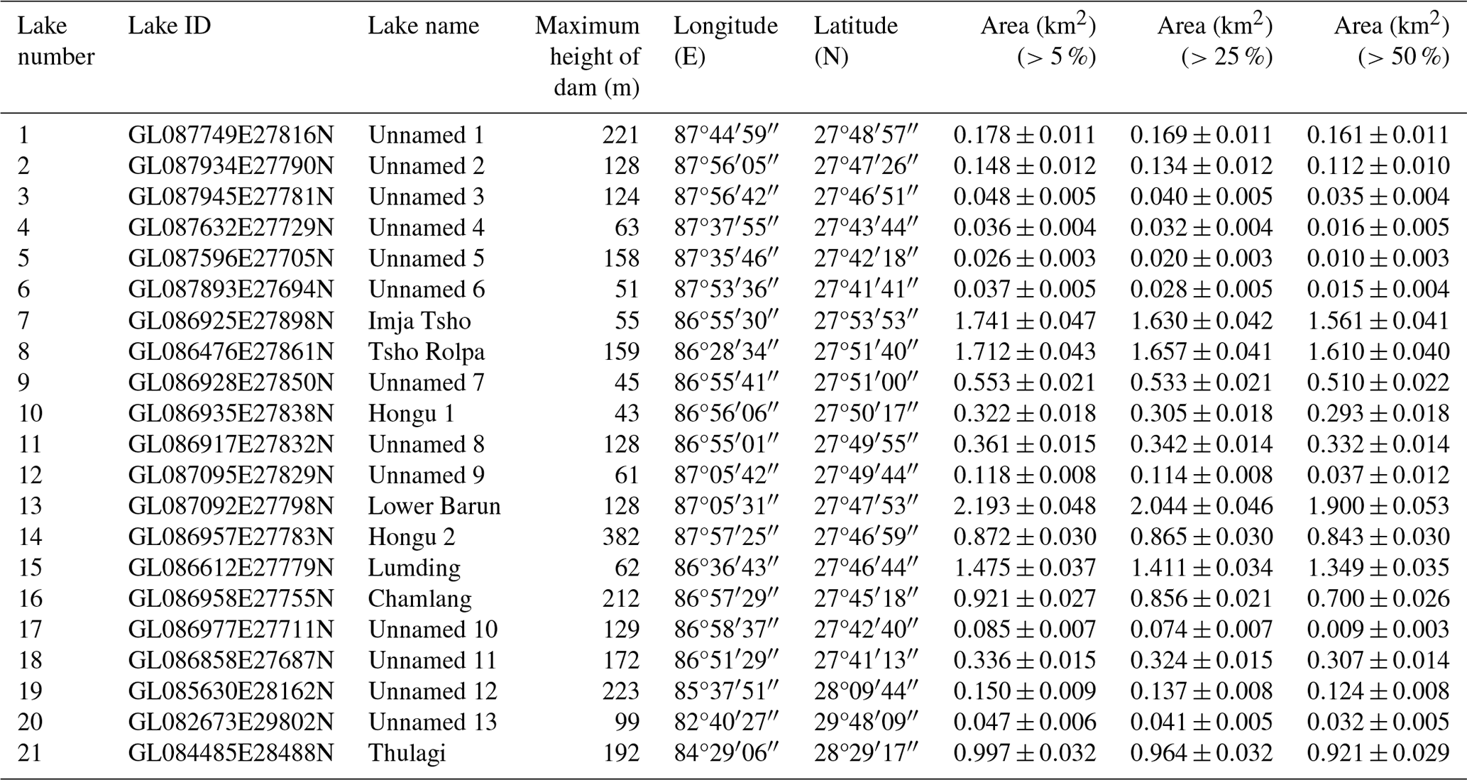
Table 1 Delineated glacial lake areas at varied water-occurrence frequencies from multi-temporal Sentinel-2 imagery.

2.2.2 Two-dimensional hydrodynamic modelling

The High-Performance Integrated Hydrodynamic Modelling System (HiPIMS) (Zhao and Liang, 2022) is employed here to simulate the breach hydrograph. HiPIMS develops a fully dynamic model based on the 2-D depth-averaged shallow water equations. The conservative form of the governing 2-D shallow water equations is expressed as follows:

$$\begin{array}{}\text{(5)}& {\displaystyle \frac{\partial \mathit{q}}{\partial t}}+{\displaystyle \frac{\partial \mathit{f}}{\partial x}}+{\displaystyle \frac{\partial \mathit{g}}{\partial y}}=\mathit{s},\end{array}$$

where t is the time, x and y represent the Cartesian coordinates, q denotes the flow-variable vector, f and g are the flux vectors in the x and y directions, and s is the source term vector. The vector terms are defined as

$$\begin{array}{}\text{(6)}& {\displaystyle }\begin{array}{rl}{\displaystyle }& {\displaystyle }\mathit{q}=\left[\begin{array}{c}h\\ q_x\\ q_y\end{array}\right],\mathit{f}=\left[\begin{array}{c}{q}_x\\ u{q}_x+\frac{\mathrm{1}}{\mathrm{2}}g{h}^{\mathrm{2}}\\ u{q}_y\end{array}\right],\\ {\displaystyle }& {\displaystyle }\mathit{g}=\left[\begin{array}{c}{q}_y\\ v{q}_x\\ v{q}_y+\frac{\mathrm{1}}{\mathrm{2}}g{h}^{\mathrm{2}}\end{array}\right],\\ {\displaystyle }& {\displaystyle }\mathit{s}=\left[\begin{array}{c}\mathrm{0}\\ -C_{f}u\sqrt{u^{\mathrm{2}}+v^{\mathrm{2}}}-gh\frac{\partial z_{\mathrm{b}}}{{\partial }_x}\\ -C_{f}v\sqrt{u^{\mathrm{2}}+v^{\mathrm{2}}}-gh\frac{\partial z_{\mathrm{b}}}{{\partial }_y}\end{array}\right],\end{array}\end{array}$$

where h is the water depth, q_x=uh and q_y=vh are the unit-width discharges in the x and y directions, u and v denote the depth-averaged velocities in two Cartesian directions, z_b is the bed elevation, and C_f is the bed roughness coefficient.

The governing equations outlined above are solved through a shock-capturing finite-volume Godunov-type scheme on uniform grids (Zhao and Liang, 2022). The numerical scheme introduces a robust Godunov-type model to deliver precise and stable predictions of overland flow and flooding processes at the catchment scale. This scheme is implemented through a Python and CUDA C hybrid programming framework to achieve multi-GPU and multi-node high-performance computing for large-scale simulations. It is worth noting that the GPU-accelerated model has demonstrated a computational efficiency of up to 10 times greater than its CPU-based counterpart (Smith and Liang, 2013). HiPIMS is set up using the terrain data and roughness data, and it is driven by the breach hydrograph for each scenario, as calculated in Sect. 2.2.1. Subsequently, the runoff is routed throughout the flow area.

2.3 GLOF exposure and impact assessment

Based on the GLOF inundation process predicted by HiPIMS for each scenario, we can estimate potential flood exposure by superimposing the exposure datasets onto the flood simulation results. In addition to assessing flood exposure, it is imperative to quantify the potential losses and impacts of GLOFs under various conditions to understand the associated risks. Estimating direct damage to buildings and other exposed objects can be done by employing appropriate depth–damage curves that establish the relationship between flood depth and potential damage. Typically, the damage is quantified as a percentage of the cost required for repairs or replacements. In this study, we utilise depth–damage curves from the HAZUS Flood model to investigate the impact of GLOFs on buildings (Scawthorn et al., 2006). Beyond buildings, GLOFs can also have a significant impact on agricultural lands and roads. We evaluate the damage to agricultural lands and roads caused by GLOFs using the damage curves recommended in a technical report published by the Joint Research Centre of the European Commission (Huizinga et al., 2017). The specific water depth–damage curves for buildings, roads, and agricultural lands used in this study can be found in Chen et al. (2022).

2.4 Data

HiPIMS is set up using a DEM to represent domain topography and land use data to parameterise domain roughness. It is driven by the out-of-breach flow discharge estimated in Sect. 2.2.1. The DEM used in this work is the Shuttle Radar Topography Mission (SRTM) DEM with a spatial resolution of 30 m (Farr et al., 2007). Land use types are extracted from the Landsat Thematic Mapper imagery from 2010 provided by the International Centre for Integrated Mountain Development (ICIMOD, 2013). The roughness of the flow area is represented by the Manning coefficient (n), which is dependent on land use types. The values assigned are 0.15 for forest, 0.035 for arable land, 0.03 for grassland, 0.027 for water surface, and 0.016 for construction land. The Manning coefficients 0.016 to 0.15 were specified based on values provided in earlier hydraulic textbooks or reports (e.g. Chow, 1959; Barnes, 1967; Arcement and Schneider, 1989), aligning with values in previous studies, e.g. 0.035 to 0.17 in Nepal (Sattar et al., 2021) and 0.035 to 0.120 in Bhutan (Rinzin et al., 2023).

Open-source datasets are used to support the assessment of GLOF exposure and impacts. The OSM is a collaborative user-generated project initiated in 2004 to provide an openly available geographical database of the world, covering both the natural and artificial environments of Earth's surface (OpenStreetMap contributors, 2022). While primarily built by volunteers, the OSM also integrates geographical data contributed by governmental and specialised GIS databases for certain areas or entire countries, e.g. Nepal, providing relatively complete spatial data on buildings and other objects. Hydropower plant data are obtained from the Hydro Map project (Nepal Hydropower Portal, 2023). In the Hydro Map project, hydropower plants are categorised into three types: operation, generation, and survey. In Nepal, the hydropower licensing regime is divided into two stages: a survey license is issued to conduct a feasibility and environmental assessment, and a generation license is granted after the project is found to be technically, environmentally, and economically viable. From the Hydro Map project, Nepal has a total of 572 hydropower projects. These projects include 81 that are currently operational, 180 with issued generation licenses, and 311 with issued survey licenses. Detailed information on each hydropower plant is provided, including the capacity, commission and issue dates, longitude, and latitude. Importing hydropower plant data into ArcGIS and comparing them with sub-metre imagery from ArcGIS Server and Google Earth, the positions of some hydropower plants are found to be inaccurate. To address the inaccuracies in the positions of some hydropower plants, a process has been undertaken to enhance the quality of the hydropower plant data. Initially, we identified all hydropower stations located within a 2 km buffer zone along the downstream rivers of glacier lakes. For licensed hydropower plants that were not situated on the river, we relocated them to the nearest river point, ensuring that they were accurately placed on the river as indicated by the Hydro Map project. For operational hydropower stations, we used high-resolution remote sensing imagery from sources such as Google Maps and Google Earth to determine their locations precisely.

3 Study area and glacial lakes

Nepal is highly vulnerable to GLOFs. A total of 53 GLOF events have been documented in Nepal from 1560 up to now (Shrestha et al., 2023). Additionally, there have been 37 GLOF events recorded in the Tibetan Autonomous Region, China, that had transboundary impacts on Nepal. These historical events have had devastating consequences for the country. For example, both the 1985 Dig Tsho GLOF and the 1998 Tam Pokhari GLOF had devastating effects, resulting in significant loss of life, property and infrastructure damage, and severe disruptions to the livelihoods of those living in downstream areas. Approximately 1.56 million people live downstream within 3 km of moraine-dammed lakes in Nepal, putting them at risk of GLOFs (Ghimire, 2004).

In Nepal, a total of 2070 glacial lakes with lake areas equal to or greater than 0.003 km² have been identified and mapped using Landsat images (Bajracharya et al., 2020). These glacial lakes are predominantly located in northern Nepal at elevations ranging from 3400 to 5908 m. Notably, 98 % of these glacial lakes are located above 4000 m. Bajracharya et al. (2020) assessed GLOF hazard factors related to lake and dam characteristics, glacier activity at the source, and the morphology of the lake surroundings for the 2070 glacial lakes. They identified 21 lakes as PDGLs (Fig. 2 and Table 1). Of the 21 PDGLs, some lakes have names, while others do not and were designated as “Unnamed”.

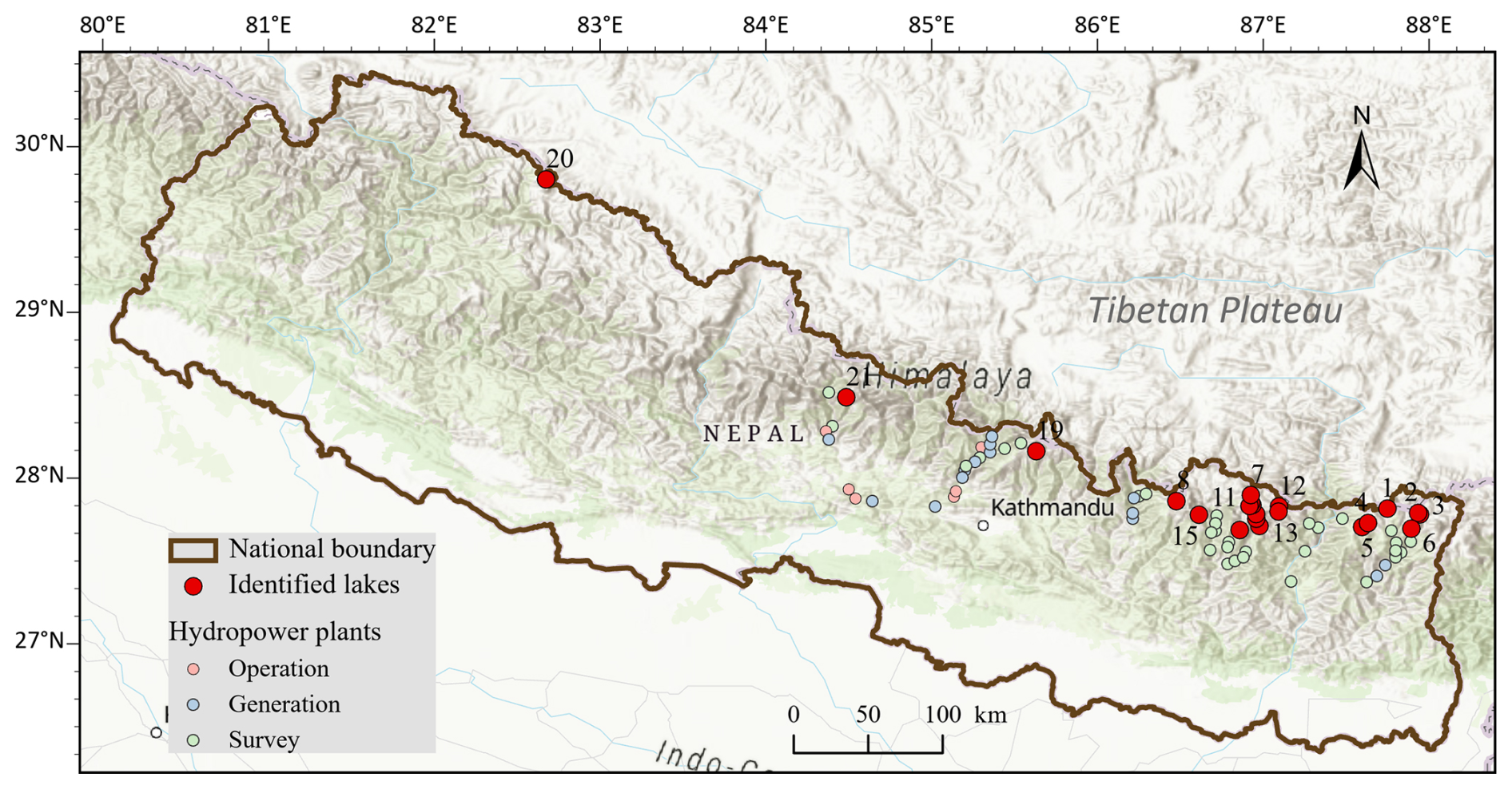
Figure 2 Study area and the 21 identified dangerous glacial lakes, each with a unique lake number and potentially impacted hydropower plants.

This study focuses on these 21 PDGLs and conducts a comprehensive assessment of their GLOF risk and downstream impacts. Each lake is assessed using the proposed evaluation framework in Sect. 2. The model and evaluation domain for each lake are determined based on the maximum potential inundation extent resulting from GLOFs as well as the topographic features and river network conditions downstream. Typically, the domain spans more than 100 km and is sufficiently extensive to encompass all potential impacts.

4 Results

4.1 Glacial lake water surface extraction

Water surfaces of glacial lakes are delineated from Sentinel-2 images using the random forest model, as previously outlined. The random forest model is trained with a set of training samples that comprise both water and non-water features. To account for seasonal variations in lake water surfaces, the training samples for water features are manually selected from images acquired at different times. Various non-water features encompass diverse landscapes and vegetation types. This training dataset is subsequently employed to drive and train the random forest model, which is then employed to delineate water surfaces for all the adopted Sentinel-2 images. The subsequent analysis involves the computation of water-occurrence frequency based on multi-temporal water surfaces. The outcomes of water-occurrence frequency for specific representative lakes are visually presented in Fig. 3. It is noteworthy that lake areas are not consistently characterised by open water throughout the year. For instance, Unnamed 1 (Fig. 3a) exhibits an average water-occurrence frequency of 72 %, while Unnamed 2 (Fig. 3b) has an average water-occurrence frequency of 58 %. In contrast, for certain lakes, like Unnamed 8 and Tsho Rolpa Lake, lake areas are always covered with water. Hence, the capacity to map glacial lakes to assess the associated GLOF risk is influenced by the timing of the image acquisition.

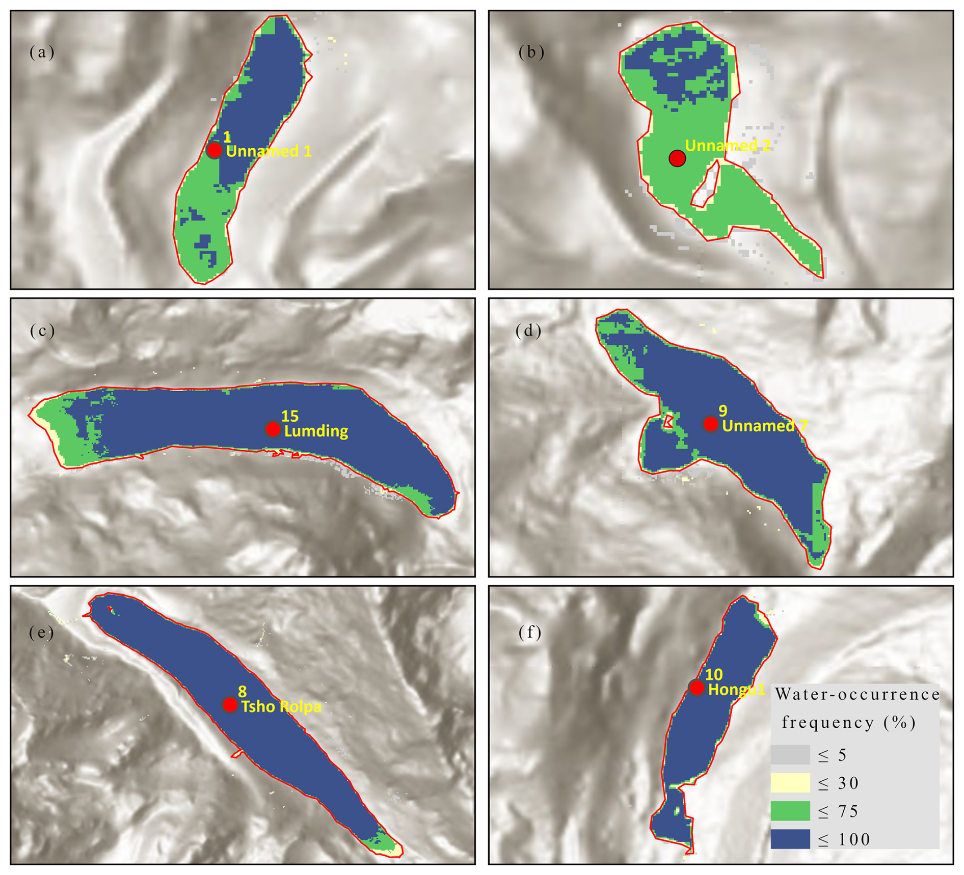
Figure 3 Water surfaces extracted from multi-temporal Sentinel-2 imagery in representative glacial lakes in Nepal (lake numbers and other lake details can be found in Table 1).

Table 1 presents the determined lake areas based on varying water-occurrence frequencies. To mitigate the effects of misinterpretations, such as cloud shadows, a 5 % threshold is utilised to exclude areas characterised by low water-occurrence frequencies. Subsequently, the maximum lake boundary is delineated for each lake, allowing for the straightforward calculation of maximum lake areas. Of the 21 lakes, the largest is Lower Barun Lake, a substantial glacial lake in Nepal known for its depth and size. Its area measures 2.193 ± 0.048 km², while the smallest lake (Unnamed 5) covers only 0.026 ± 0.003 km². Lower Barun Lake, along with the second largest PDGL, Imja Tsho Lake, has undergone significant area growth. The estimated maximum area of Imja Tsho Lake here is 1.741 ± 0.047 km². Tsho Rolpa Lake boasts a maximum area estimated at 1.712 ± 0.043 km². This aligns with previous findings, which reported that the lake had an area of 0.23 km² in 1957, which grew to 1.02 km² in 1979, 1.65 km² in 1999, and 1.61 km² in 2019 (Chen et al., 2022). Lumding Lake, another PDGL with an estimated area exceeding 1 km², displayed notable growth. It had an area of 0.104 km² in 1963, 0.66 km² in 1987, 0.8 km² in 1996, and 1.18 km² in 2016 (Khadka et al., 2019). Our assessment indicates that the maximum area of Lumding Lake is 1.475 ± 0.037 km². In summary, the estimated maximum lake areas derived from multi-temporal satellite images for these extensively studied lakes are in good agreement with previous research. To establish the maximum lake boundary for potential risk assessment, it is imperative to leverage multi-temporal imagery capturing various hydrological conditions of glacial lakes.

The maximum areas of the four large lakes (Lower Barun, Imja Tsho, Tsho Rolpa, and Lumding), each exceeding 1 km², are approximately 1.1 times the extent of the area that water covers more than 50 % of the time. In contrast, for the comparatively smaller lakes (Unnamed 3, 4, 5, 6, 10, and 13), the ratio of the maximum area to the area covered by water for more than 50 % of the time can be as high as 1.4 to 2.5 times. For instance, Unnamed 10 has a maximum area of 0.085 km², while only 0.009 km² is covered with water more than 50 % of the time. The areas of small PDGLs exhibit more significant variations in space and time compared to those of larger PDGLs, making the associated risks more uncertain.

4.2 Lake volumes and peak discharge prediction

We obtained 94 estimates of the total volume V_tot (Fig. 4a) and flood volume V₀ under a complete breach of dam height (Fig. 4b) for each lake and a total of 940 000 scenarios of peak discharge Q_p per lake (Fig. 4c) using the models introduced in Sect. 2.2.1. Figure 4a clearly illustrates the variation in total volumes among the 21 PDGLs, with Lower Barun (number 13) standing out as the most substantial one, possessing a median value of approximately 208.2×10⁶ m³. In contrast, Unnamed 5 (number 5) is the smallest one, with a median volume of approximately 204.0×10³ m³. The disparity between these two lakes is striking, as Lower Barun's median volume is approximately 1000 times greater than that of Unnamed 5. We collected geophysical investigation data for named PDGLs and compared them against calculated volumes using field-investigated lake areas, as shown in Table 2. While there are some inconsistencies, the calculated volumes generally align with the investigated values. For example, the water volume of the glacial Lower Barun Lake in 2015 was approximately 112.3×10⁶ m³, with a lake area of 1.52 km² based on bathymetric measurements. Using the established relationship between lake area and volume, the average volume for a lake with a 1.52 km² area is calculated to be 108.27×10⁶ m³, which closely matches the measured volume of the glacial Lower Barun Lake.

Figure 4 (a) Estimated total volume, (b) flood volume under the complete breach of dam height, and (c) peak discharge for each glacial lake.

Table 2 Comparisons between the lake areas (km²) and volumes (10⁶ m³) derived from bathymetric investigations and those calculated in this study for the named lakes.

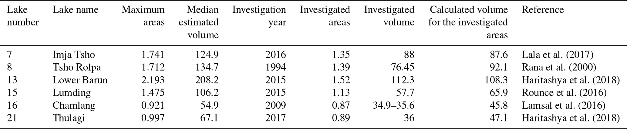
Figure 4b highlights the substantial variation in potential flood volumes across the lakes in the theoretically most extreme scenarios, i.e. a complete breach of dam height with Lower Barun exhibiting the highest median flood volume and Unnamed 5 having the lowest median flood volume. Notably, the median flood volume of Lower Barun is approximately 1160 times greater than that of Unnamed 5. According to Fig. 4c, which shows the distribution of peak discharges, Lower Barun has the highest median peak discharge at 21.3×10³ m³ s⁻¹. Following it are Lumding, Imja Tsho, and Tsho Rolpa, which have similar peak discharge magnitudes ranging from 13 000 to 15 000 m³ s⁻¹. The lake with the lowest peak discharge is Unnamed 6, with a discharge of 154.1 m³ s⁻¹. The peak discharge of Lower Barun is approximately 140 times greater than that of Unnamed 6.

4.3 Flood inundation simulation

4.3.1 Inundation areas

HiPIMS is used to simulate flood dynamics in 100 scenarios for each lake with its maximum dam height breached. The final flood inundation probability and maximum water depth are derived from each scenario's results multiplied by their respective weights. Herein, we use the simulation results from Imja Tsho Lake and Lower Barun Lake as illustrative examples (Fig. 5). The areas with high flood inundation probabilities are predominantly distributed along the downstream valley. The areas with flood inundation frequencies exceeding 5 % can be substantial, reaching 95.6 km² for Imja Tsho Lake and 200.4 km² for Lower Barun Lake. The maximum water depth offers spatial insights into the potential severity of GLOFs in downstream areas (Fig. 5c and d). It facilitates the identification of areas characterised by both high inundation probability and significant maximum water depth. For instance, for Lower Barun Lake, there are 127.4 km² of areas exhibiting both an inundation frequency exceeding 90 % and a maximum water depth exceeding 0.5 m. These specific areas should undoubtedly receive heightened attention in future flood risk management and mitigation.

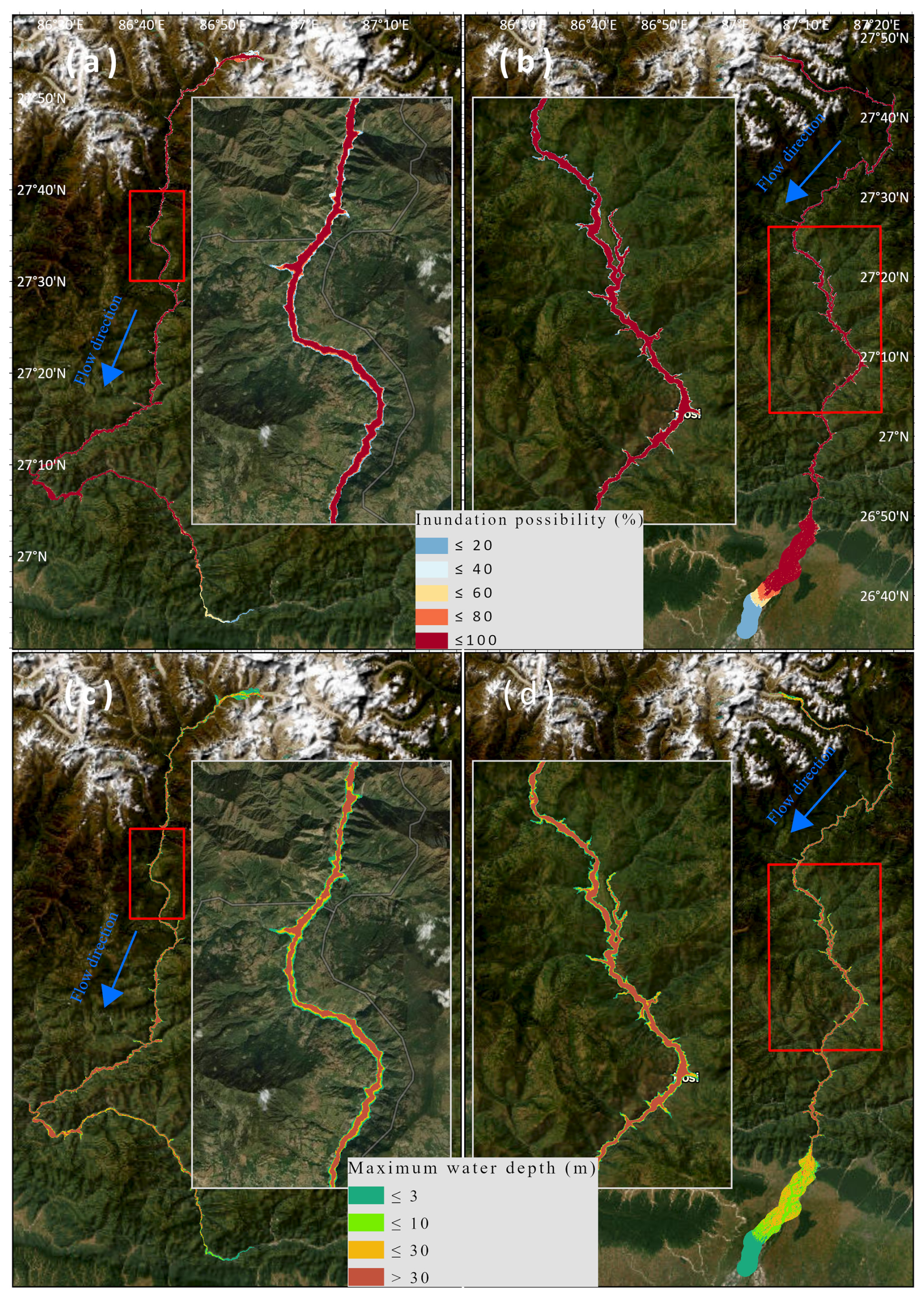
Figure 5 GLOF inundation probability for (a) Imja Tsho Lake and (b) Lower Barun Lake, together with the maximum water depth for (c) Imja Tsho Lake and (d) Lower Barun Lake, in the theoretically worst situation, i.e. complete breach of dam height. (The basemaps used were accessed from ArcGIS Online Basemap provided by Esri.)

The resulting inundation areas at different levels of inundation probabilities are shown in Fig. 6. The inundation extent resulting from GLOFs originating from the 21 PDGLs ranges from 3.6 to 200.4 km². Notably, the largest glacial lake, Lower Barun (lake number 13), has inundation areas of 172.4 and 189.5 km² for inundation probabilities exceeding 75 % and 50 %, respectively. Tsho Rolpa (lake number 8), having a smaller lake area than Lower Barun, projects inundation areas of 106.9 and 120.3 km² for probabilities exceeding 75 % and 50 %, respectively. Imja Tsho Lake (lake number 7), similar in size to Tsho Rolpa Lake, anticipates inundation areas of 67.2 and 79.6 km² for probabilities exceeding 75 % and 50 %, respectively. It is worth noting that lakes that have not been extensively studied can potentially cause large inundation areas of over 10 km² for probabilities exceeding 50 %, including Unnamed 7, Unnamed 8, Unnamed 11, Unnamed 12, Unnamed 1, and Unnamed 2. The smallest lake, Unnamed 5, has an inundation area of 2.7 km² for probabilities exceeding 50 %.

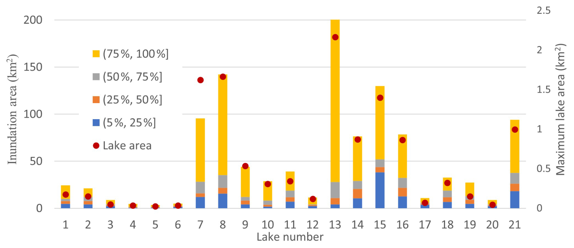
Figure 6 Inundation area (km²) at different levels of inundation probabilities and maximum lake area (km²).

To comprehensively evaluate all potential glacial lake outburst scenarios, we also consider less severe conditions, specifically where 10 %, 30 %, and 50 % of dam heights are breached. In each of these scenarios, 100 representative cases are selected from a total of 940 000 samples using k-means clustering. The outcomes of these less severe scenarios are then compared to the condition of 100 % of the dam height breached. Figure 7 illustrates the inundation areas for probabilities exceeding 5 % due to GLOFs. For Lower Barun Lake, breaches reaching 10 % and 30 % of the dam height result in inundations of 25.5 and 131.0 km² of downstream areas. When 100 % of the dam height is breached, the inundation areas are 7.87 and 1.53 times larger than those observed in the 10 % and 30 % scenarios, respectively. Following Lower Barun Lake, Tsho Rolpa Lake and Lumding Lake also present substantial inundation risks. Even at 10 % of the dam height breached, Tsho Rolpa Lake has the potential to inundate approximately 40 km² of areas with inundation probabilities exceeding 5 %.

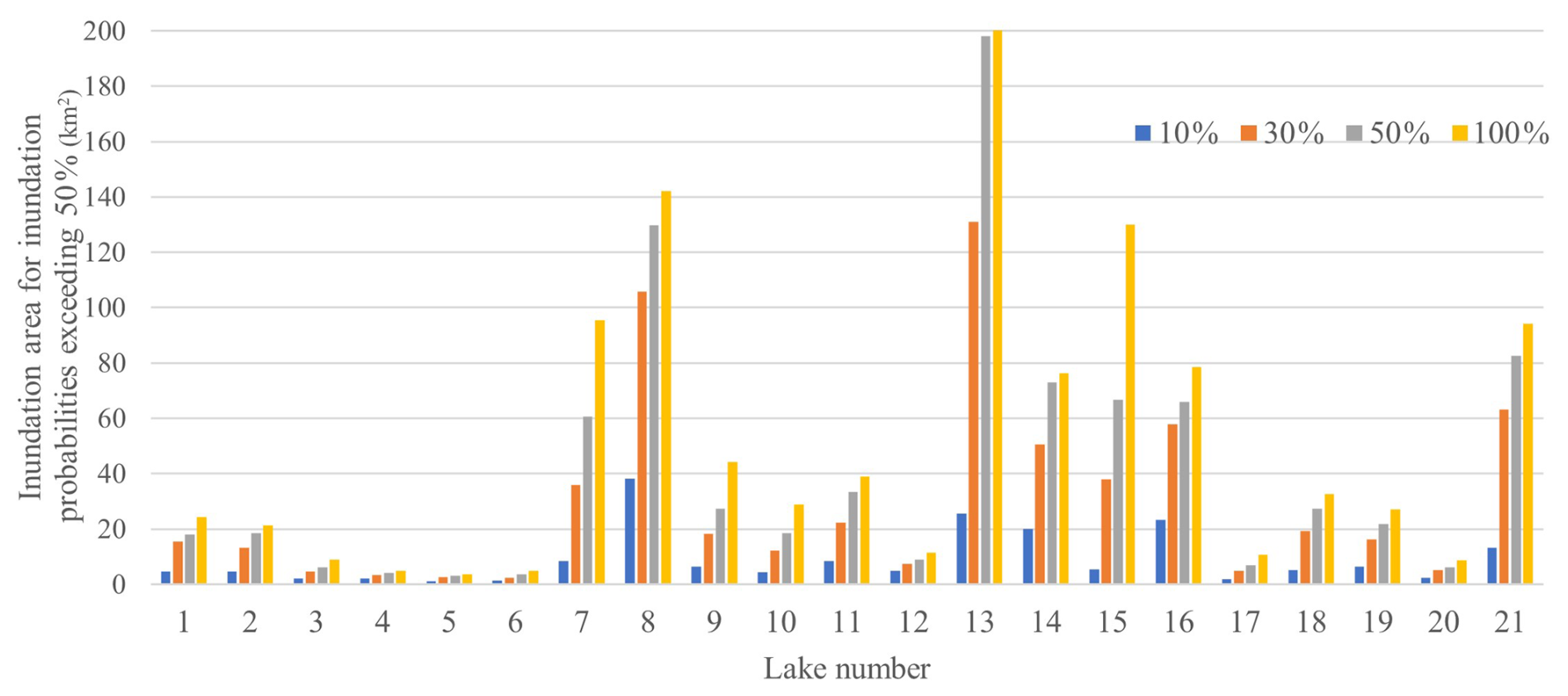
Figure 7 Inundation area (km²) for inundation probabilities exceeding 5 % under 10 %, 30 %, 50 %, and 100 % of dam heights breached.

4.3.2 Exposure assessment

The exposure of objects can be determined spatially by overlaying the predicted flood inundation maps with relevant datasets detailing buildings, roads, and agricultural land (Table 3). Here, we focus on areas with flood probabilities greater than 5 %. The number of inundated buildings varies from 11 to 34 715. Out of the 21 PDGLs, 14 have a number of inundated buildings exceeding 100, while 8 of them inundate at least 1000 buildings. The three lakes with the highest number of inundated buildings are Thulagi, Tsho Rolpa, and Lower Barun, each of which could inundate more than 5000 buildings and cover an area of 3.7×10⁵ m² of building areas. The numbers of buildings inundated by Tsho Rolpa and Thulagi are 1.7 and 2.5 times that of Lower Barun Lake. Overall, these well-studied lakes could impact more buildings than unnamed lakes. These 13 unnamed lakes typically affect fewer than 300 buildings, with the exceptions being Unnamed 1 and Unnamed 12, which can influence 310 and 1659 buildings, respectively. Six unnamed lakes, i.e. Unnamed 12, 1, 7, 11, 8, and 2, have the potential to impact more than 200 buildings. Further investigation and research are required for the six unnamed lakes. Conversely, three lakes, i.e. Unnamed 10, Unnamed 6, and Unnamed 9, pose lower risks, with a number of 15 or fewer buildings affected.

Table 3 GLOF induced inundation areas and damage extents to buildings, roads, and agricultural lands under 100 % of dam height breached.

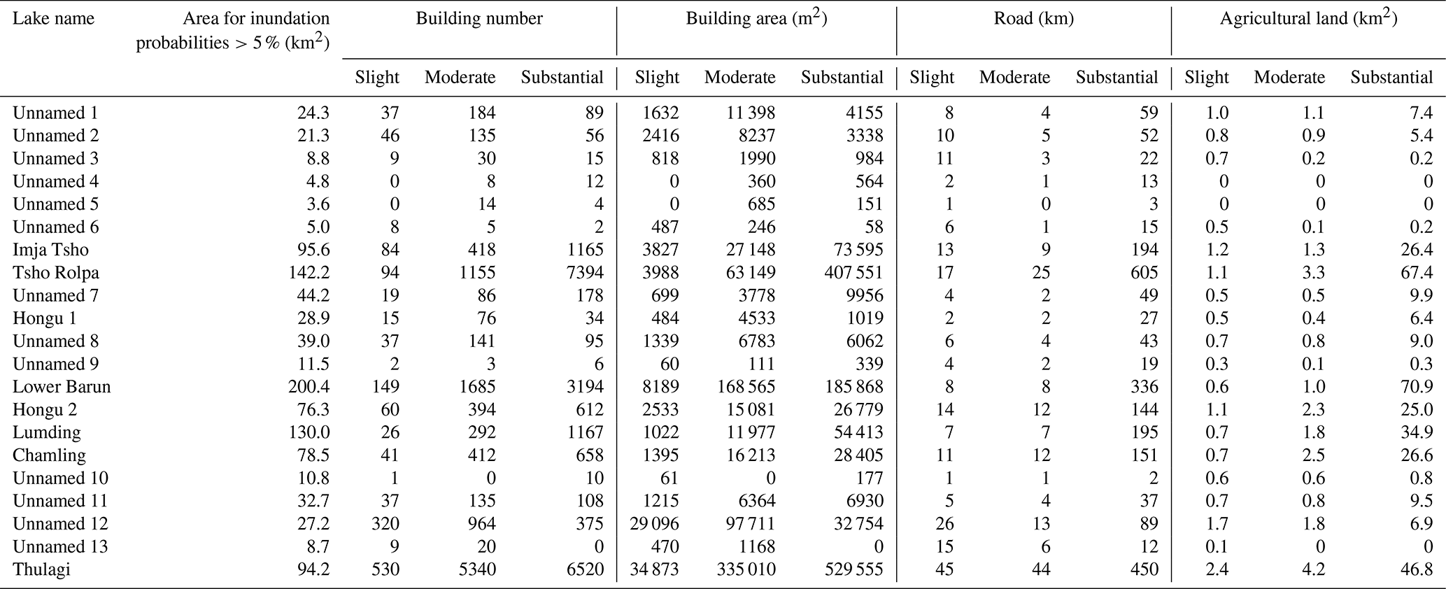
Regarding inundated roads, the value ranges from 4 to 646 km. Tsho Rolpa, Thulagi, and Lower Barun still hold the top three positions with the greatest lengths of inundated roads, each exceeding 350 km. To illustrate this, Tsho Rolpa Lake, the top one in this category, inundates a 646 km long road. Following closely is Thulagi Lake, which has inundated roads with a length of 539 km. Agriculture is a cornerstone of the Nepalese economy, and it is susceptible to the impacts of GLOFs. It is anticipated that 12 lakes will have more than 10 km² of inundated agricultural land and that 3 lakes will have a negligible impact on agriculture. Lower Barun, Tsho Rolpa, and Thulagi are still the most perilous lakes in terms of the inundation of agricultural lands.

In addition to the high potential for human settlements to be exposed to GLOFs, hydropower projects are increasingly vulnerable to these events. A total of 49 hydropower plants (as shown in Fig. 2, with detailed information provided in Table S1 in the Supplement) have been identified as being in close proximity to GLOF flow channels, thereby rendering them potentially vulnerable to GLOFs associated with the 21 PDGLs. Of these, five plants are currently operational. Additionally, 44 hydropower plants, for which generation or survey licenses have been issued, are also exposed to the risk of GLOFs from these 21 PDGLs. When examining the potential impact of lakes on operational hydropower plants and those holding generation licenses, it is observed that Thulagi and Tsho Rolpa pose a risk of inundating five plants (three operational ones and two licensed ones) and three plants (all licensed), respectively. Moreover, it is noteworthy that Unnamed 12, Unnamed 1, and Unnamed 2 have the potential to inundate seven plants (two operational and six licensed), two plants (both licensed), and two plants (both licensed), respectively.

4.3.3 Damage assessment

GLOF damage assessment relies on spatial inundation maps of water depth and depth–damage curves. The inundation maps, depicting water depth, are represented by maximum water depths for areas with flood probabilities greater than 5 %. Following the technical manual of the HAZUS Flood model (FEMA, 2009), damage extents of 1 % to 10 %, 11 % to 50 %, and 50 % to 100 % are defined as slight, moderate, and substantial damage, respectively. Figure 8 uses Unnamed 12 as an example to illustrate the spatial distribution of damage to buildings, roads, and agricultural land caused by GLOFs. Table 3 provides estimates of damage to buildings, roads, and agricultural lands for each lake. In the case of Tsho Rolpa, 7394 buildings are projected to suffer substantial damage from GLOFs. Thulagi Lake and Lower Barun Lake are expected to cause substantial damage to 6520 and 3194 buildings, respectively. Other lakes, such as Imja Tsho Lake and Lumding Lake, are estimated to impact roughly 1160 buildings with substantial damage. Notably, Unnamed 12 has the potential to affect 1659 buildings, with 964 experiencing moderate impact and 375 facing substantial damage. Situated in the Trishuli River basin, Unnamed 12 faces high exposure. On the other hand, another unnamed lake (Unnamed 13) is not projected to cause any substantial damage to buildings due to GLOFs. For PDGLs with a high number of impacted buildings (more than 1000), except for Unnamed 12, more than 50 % of the impacted buildings are expected to incur substantial damage. In all the PDGLs, most affected buildings (over 60 %) are predicted to experience moderate or substantial damage. Likewise, over 60 % of roads and agricultural lands are anticipated to undergo moderate or substantial damage due to high levels of maximum water depth.

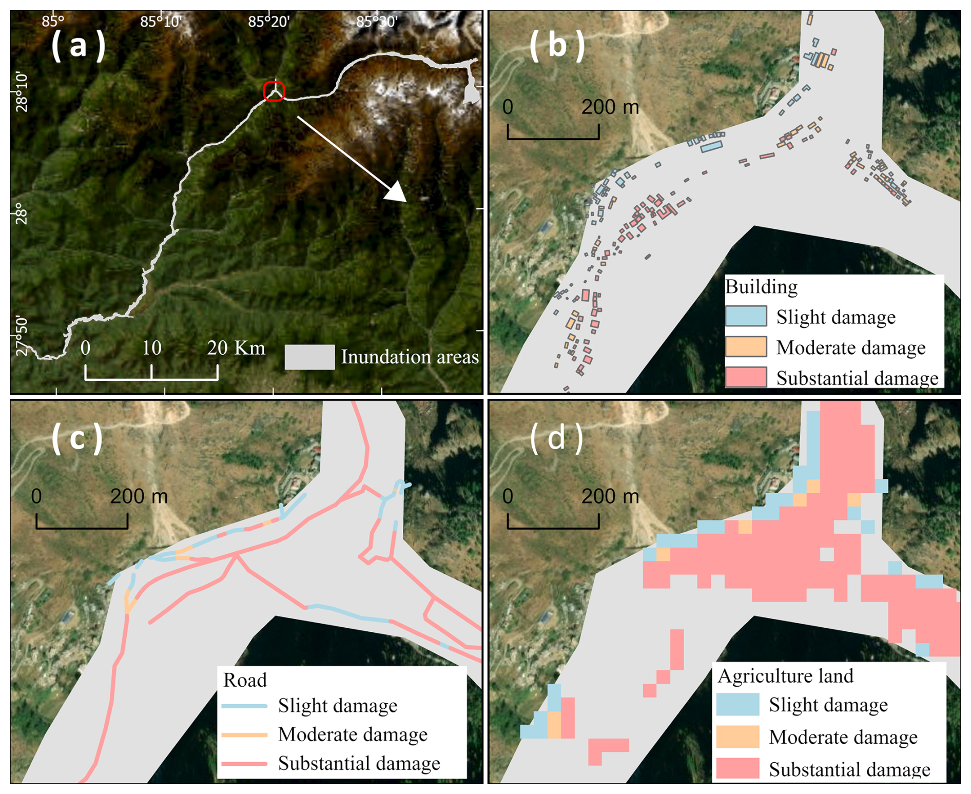
Figure 8 Damage to buildings, roads, and agricultural land caused by the theoretically most serious GLOF due to Unnamed 12 (basemap sources: Earthstar Geographics and Maxar).

5 Discussion

We evaluate GLOF scenarios involving breaches of 10 %, 30 %, 50 %, and 100 % of dam heights. It is recognised that, for certain lakes, a complete (100 %) breach may be improbable and represents only a theoretical worst-case scenario. In practical terms, the most severe realistic scenario should consider the unique lithology, composition, and structural characteristics of each moraine dam; however, conducting such detailed field investigations to gather this information across multiple lakes at a large scale remains challenging. For large-scale GLOF risk assessments, Zhang et al. (2023b) applied an empirical relationship between lake volume and flood volume, derived from historical GLOFs, to estimate flood volumes, capping the maximum flood volume at 20×10⁶ m³ due to limited data on large glacial lakes. Fujita et al. (2013) estimated potential flood volume by analysing the depression angle from lake shorelines using DEM data, noting that potential flood volume is helpful for preliminarily identifying and prioritising lakes for further investigation, but it does not directly quantify GLOF risk. As no straightforward and reliable method currently exists for accurately predicting flood volumes across multiple lakes, we analysed scenarios assuming breaches at 10 %, 30 %, 50 %, and 100 % of dam heights for consistency. When interpreting these impact results, the inherent limitations in predicting flood volume and the realistic likelihood of each scenario should be considered carefully.

GLOFs can have a significant impact due to the large volume of water stored in glacial lakes, resulting in rapid breaches, high outflow peaks, and high total discharges. While there is a positive correlation between inundation extent and lake area (Fig. 6), it is important to note that inundation propagation and extent also depend on dam breach processes as well as the underlying topography and land surface conditions of downstream areas (Worni et al., 2012; Ancey et al., 2019). In particular, steep and narrow valley gorges can influence flood waves, causing them to spread rapidly over long distances, which is often accompanied by significant physical processes such as erosion and the transport of ice, sediment, and debris. Of the 21 PDGLs in Nepal, Tsho Rolpa Lake, Thulagi Lake, and Lower Barun Lake are expected to experience the most severe impacts of GLOFs on buildings, roads, and agricultural areas. Rounce et al. (2016, 2017) also assessed the downstream impacts of GLOFs from glacial lakes in the Nepalese Himalayas. They likewise identified Tsho Rolpa Lake, Lower Barun Lake, and Thulagi Lake as having the most affected buildings, while two unnamed lakes and Thulagi Lake were anticipated to experience the most significant impacts on agricultural areas. However, it is important to note that Rounce et al. (2016, 2017) employed the Monte Carlo least-cost path model (Watson et al., 2015) to estimate the extent of GLOFs for each lake. While the model is computationally efficient and suitable for large-scale applications, it lacks a physical basis and relies solely on the terrain conditions downstream along the river channel, without considering variations in lake release volumes and peak discharges. As a result, flood extents for lakes with differing potential flood volumes may be indistinguishable. Another limitation is that the threshold for the cut-off distance in the Monte Carlo least-cost path model needs to be set artificially, while the realistic cut-off distance downstream for each lake varies, sometimes extending over 200 km downstream (Richardson and Reynolds, 2000). This study takes a different approach by employing a physics-based hydrodynamic model that predicts not only the inundation extent, but also the spatial characteristics of flood features, including inundation probabilities and water depth, while considering various outburst scenarios. This information can be used to identify potential exposures and assess the extent of damage to which exposures may be subject.

In addition to the growing vulnerability of human settlements in mountainous regions, there is increasing exposure to GLOFs of infrastructure related to energy security and commerce. Therefore, an objective assessment of the risk to infrastructure posed by PDGLs is crucial. This study considers hydropower plants, given their critical importance and rapid development in Nepal. Nepal is at the heart of a modern resurgence in hydropower development in the Himalayas (Lord, 2016). The country boasts abundant hydropower resources thanks to its ample river water, steep gradients, and mountainous terrain. At present, a considerable number of hydropower projects are in the planning and construction stages (46 projects exceeding 100 GW) to enhance the country's overall generating capacity. These planned hydropower projects are primarily situated along rivers connected to glaciers located in the northern region of Nepal (Shakti et al., 2021). A few existing hydropower plants have experienced direct impacts from recorded GLOFs, such as the Namche hydroelectric power plant destroyed by the 1985 Dig Tsho GLOF (Vuichard and Zimmermann, 1987) and the Bhotekoshi hydropower plant affected by the 2016 GLOF (Cook et al., 2018), so GLOFs can be highly destructive and unpredictable, posing a significant threat to hydropower facilities. Furthermore, the expansion of hydropower plants into the upstream regions of watersheds substantially increases the vulnerability of infrastructure to GLOFs (Nie et al., 2021). Schwanghart et al. (2016) estimated that two-thirds of the existing and planned hydropower projects in the Himalayas are located in areas potentially affected by GLOFs, and up to one-third of these projects could face GLOF discharges exceeding their local design flood capacities. In this study, we have identified 49 existing and planned hydropower projects that could potentially be impacted by GLOFs originating from the 21 PDGLs; however, we did not assess the specific impacts of GLOFs on these hydropower projects. To our knowledge, there are no readily available damage curves that correlate the potential impact on hydropower plants with flood depth and other flood characteristics. Furthermore, hydropower plants typically comprise multiple components, including dam and reservoir, powerhouse, and auxiliary facilities. The spatial extent of a hydropower plant can vary significantly, ranging from a few square kilometres to several hundred square kilometres. Accurate assessment would require detailed spatial information and mapping of hydropower plants, which is currently lacking. Consequently, this study focuses exclusively on identifying whether a hydropower plant is potentially at risk from GLOFs without engaging in a detailed assessment of the specific damages that may be incurred. Still, we urge stakeholders responsible for planning, designing, constructing, and managing infrastructure to consider these potential GLOF risks.

In addition to well-studied PDGLs like Tsho Rolpa Lake, Thulagi Lake, and Lower Barun Lake, some unnamed lakes also present a significant risk of GLOFs. For instance, Unnamed 12, 1, 7, 11, 8, and 2 pose high GLOF risks. GLOFs from any of these six lakes have the potential to impact more than 200 buildings, and GLOFs resulting from Unnamed 12 may submerge existing hydropower facilities. Unfortunately, there is limited information available about these unnamed lakes in comparison to well-studied PDGLs. To gain a better understanding of their conditions, a comprehensive research strategy is needed, which includes fieldwork investigations, remote sensing techniques, and modelling approaches. This study has leveraged remote sensing techniques and modelling approaches to preliminarily identify PDGLs with a high level of exposure and potential impacts from GLOFs. However, it is imperative to conduct fieldwork investigations, including in situ measurements, to obtain the essential information required to comprehend the actual state of these unnamed lakes at the local scale. These field investigations will also serve as a ground truth to calibrate remote-sensing-based data and model outputs. Moreover, considering the challenging nature of fieldwork in glacial lake areas, the cost of expeditions, and the high level of fitness and expertise required by monitoring teams, the preliminary identification of PDGLs with high exposure and potential impacts can offer valuable evidence to support decision-making in the allocation of financial and human resources.

We acknowledge the importance of validating the proposed framework for estimating the impact of GLOFs while recognising the inherent challenges associated with validation due to the limited availability of historical data. Although Nie et al. (2018), Veh et al. (2019), and Shrestha et al. (2023) provided valuable inventories of historical GLOFs in the Himalayas, these primarily provide information on the dates and locations of outbursts, offering limited or no information on the actual impacts resulting from historical GLOFs. Even when impact data are available, they often only comprise generalised descriptions, encompassing metrics like the overall number of casualties, infrastructure damage, and affected villages and lacking specific spatial information. Consequently, obtaining adequate data for validating our proposed impact estimation framework for GLOFs proves challenging. It is noteworthy that our proposed framework employs the fully physically based hydrodynamic model HiPIMS, which is intricately designed to capture the highly transient and complex hydrodynamic processes induced by events such as dam breaks and flash floods. HiPIMS has been validated successfully for these extreme flow conditions (e.g. Smith and Liang, 2013; Liang et al., 2016). The adoption of this model enhances our confidence in simulating the spatial–temporal processes of GLOF inundation, ultimately contributing to improved hazard evaluation results. Furthermore, we employ Bayesian approaches to derive plausible value ranges for lake volumes and peak discharges. These approaches facilitate the creation of multiple GLOF scenarios for each glacial lake, ensuring comprehensive coverage of all potential glacial lake outburst scenarios. The incorporation of Bayesian methods allows us to account for uncertainties, thereby enhancing the robustness of our impact evaluation for potentially devastating GLOFs.

6 Conclusion

Exposure and damage estimations are integral components of GLOF risk assessment. Having sufficient information on the potential impacts of GLOFs originating from PDGLs is essential for facilitating GLOF risk management. In this study, we harnessed multi-temporal satellite imagery, Bayesian regression models that establish relationships between lake areas and depths as well as between flood volume and peak discharge, and a high-performance hydrodynamic flood model to support GLOF exposure and damage assessments for multiple lakes. We applied this assessment framework to 21 PDGLs identified in the Nepalese Himalayas, and the key findings of this study are summarised as follows:

• Utilising multi-temporal imagery capturing different hydrological conditions of glacial lakes enables derivation of the full or maximum glacial lake boundaries for potential risk assessment.

• The Bayesian regression model, which establishes relationships between lake areas and depths as well as between flood volume and peak discharge, can produce predictive posterior distributions for lake depths and peak discharges for each lake. These distributions offer a plausible range of values for lake volumes and peak discharges for each PDGL, facilitating subsequent objective flood modelling and impact analysis.

• The hydrodynamic model (HiPIMS), supported by parallelised high-performance GPU computation, is capable of predicting the resulting GLOFs in terms of temporally and spatially varying flood frequency and water depths to reflect the highly transient flood dynamics in various scenarios for multiple glacial lakes on a large scale.

• Of the 21 PDGLs identified in the Nepalese Himalayas, in the scenario of a complete breach of dam height, Tsho Rolpa Lake, Thulagi Lake, and Lower Barun Lake are poised to bear the most severe impacts of GLOFs on buildings, roads, and agricultural areas. Six unnamed lakes, specifically Unnamed 12 in the Trishuli River basin, Unnamed 1 and Unnamed 2 in the Tamor River basin, and Unnamed 7, 8, and 11 in the Dudh River basin, have the potential to impact more than 200 buildings. The GLOFs from these 21 PDGLs can also impact the 5 existing hydropower plants and the 44 hydropower projects that have been granted generation or survey licenses. Notably, Unnamed 12 in the Trishuli River basin may even submerge existing hydropower facilities.

Appendix A: List of abbreviations used in this study

CI	Confidence interval
DEM	Digital elevation model
EVI	Enhanced Vegetation Index
GIS	Geographic Information System
GLOFs	Glacial lake outburst floods
GPU	Graphics processing unit
HDI	Highest density interval
HiPIMS	High-Performance Integrated Hydrodynamic Modelling System
MNDWI	Modified Normalized Difference Water Index
NIR	Near-infrared
NDMI	Normalized Difference Moisture Index
NDVI	Normalized Difference Vegetation Index
NDWI	Normalized Difference Water Index
OSM	OpenStreetMap
PDGL	Potentially dangerous glacial lake
SRTM	Shuttle Radar Topography Mission
TOA	Top of atmosphere