Understanding the relationship between streamflow forecast skill and value across the western US

Accurate seasonal streamflow forecasts are essential for effective decision-making in water management. In a decision-making context, it is important to understand the relationship between forecast skill – the accuracy of forecasts against observations – and forecast value, which is the forecast's economic impact assessed by weighing potential mitigation costs against potential future losses. This study explores how errors in these probabilistic forecasts can reduce their economic “value,” especially during droughts, when decision-making is most critical. This value varies by region and is contextually dependent, often limiting retrospective insights to specific operational water management systems. Additionally, the value is shaped by the intrinsic qualities of the forecasts themselves. To assess this gap, this study examines how forecast skill transforms into value for true forecasts (using real-world models) in unmanaged snow-dominated basins that supply flows to downstream managed systems. We measure forecast skill using quantile loss and quantify forecast value through the potential economic value framework. The framework is well-suited for categorical decisions and uses a cost-loss model, where the economic implications of both correct and incorrect decisions are considered for a set of hypothetical decision-makers. True forecasts are included, made with commonly used models within an ensemble streamflow prediction (ESP) framework using a process-based hydrologic modeling system, WRF-Hydro, and a deep-learning model, Long Short-term Memory Networks, as well as operational forecasts from the NRCS. To better interpret the relationship between skill and value, we compare true forecasts with synthetic forecasts that are created by imposing regular error structures on observed streamflow volumes. We assess the sensitivity of skill and value from both synthetic and true forecasts by modifying fundamental properties of the forecast-error in mean and change in variability. Our findings indicate that errors in mean and change in variability consistently explain variations in forecast skill for true forecasts. However, these errors do not fully explain the variations in forecast value across the basins, primarily due to irregular error structures, which impact categorical measures such as hit and false alarm rates, causing high forecast skill to not necessarily result in high forecast value. We identify two key insights: first, hit and false alarm rates effectively capture variability in forecast value rather than error in mean and change in variability; second, the relationship between forecast skill and value shifts monotonically with drought severity. These findings emphasize the need for a deeper understanding of how forecast performance metrics relate to both skill and value, highlighting the complexities in assessing the effectiveness of forecasting systems.

1 Introduction

Probabilistic seasonal streamflow forecasts are essential for informed decision-making in water resource management, including flood risk mitigation, agriculture, energy production, and in-stream ecosystem services. These forecasts enable stakeholders to plan for optimal water allocation, optimize reservoir operations, and prepare for extreme hydrologic events like droughts or floods (Wood et al., 2015). However, in an increasingly complex economy with a growing and diverse user base, the relationship between forecast skill – the accuracy of the forecast – and the forecast value – the forecast's impact on decision-making and economic outcomes – is far from straightforward (Crochemore et al., 2024). Forecast value is influenced by such factors as the cost of taking preventive action (e.g., investing in crop insurance), the potential losses from incorrect decisions (e.g., economic losses due to over- or under-allocation of water resources), and the context of decision-making (e.g., hiring labor for an agricultural entity). This relationship is complex and varies by region, often restricting the retrospective insights gained to specific operational systems. As a result, there is limited understanding of the link between skill and value – especially concerning the quality of forecasting systems. The complexity of forecast value can be framed within simple economic models like the cost–loss ratio framework. In this model, decision-makers face a potential loss if an adverse event (e.g., a drought) occurs but can take preventive action at a cost to mitigate this loss. Understanding how forecast skill translates into forecast value is critical, as it highlights the importance of not only improving the accuracy of forecasts but also understanding how skill impacts decision-making outcomes. This study addresses the following research question: how do errors in different forecasting systems affect forecast skill and decision-making value in unmanaged basins, and how can these insights guide improvements in forecast systems?

1.1 Forecast skill of probabilistic seasonal streamflow forecasts has evolved

Probabilistic seasonal streamflow forecasts estimate the likelihood of different streamflow signatures over a given period, using various approaches, such as process-based models, data-driven models, historical data, or climate forecasts, or a combination of these approaches. Probabilistic seasonal streamflow forecasts have become a crucial tool in water resources management (Crochemore et al., 2016; Ficchì et al., 2016; Kaune et al., 2020; Turner et al., 2017; Watts et al., 2012), as they provide a range of possible outcomes rather than a single deterministic prediction (Demargne et al., 2014). This probabilistic approach helps decision-makers quantify forecast uncertainty, enabling more informed and flexible water management strategies (Pagano et al., 2014). For example, the Natural Resources Conservation Services (hereafter, “NRCS”) forecasts have been widely used for water management and agricultural planning (Fleming et al., 2021).

Ensemble streamflow prediction (ESP) is a hydrologic forecasting method that generates multiple streamflow simulations using historical meteorological data as inputs to a hydrologic model (Day, 1985). Over time, ESP methods have significantly evolved in predicting water volumes through advances in hydrologic modeling, the incorporation of outputs from dynamical meteorological and climate models, and the adoption of more sophisticated forecasting methods (Clark et al., 2016; Li et al., 2017). Key developments include better representation of watershed processes in hydrologic models and the use of data assimilation techniques (Wood and Lettenmaier, 2006). Furthermore, the application of machine learning algorithms, such as the popular long short-term memory (LSTM) algorithm, has become instrumental in detecting complex patterns in data, leading to even greater refinement in forecast accuracy when combined with improved meteorological inputs (Modi et al., 2024; Mosavi et al., 2018). Among the various methods, the US National Water Model (NWM) stands out as a state-of-the-art process-based forecasting framework, which provides high-resolution operation streamflow forecasts across the continental US (CONUS) by incorporating improved hydrologic representation and real-time meteorological data to enhance forecast skill (Cosgrove et al., 2024). However, the model has limitations in certain regions, such as parts of the Intermountain West, where forecast skill remains a challenge. This study will test some of these methods, evaluating their effectiveness and applicability across various scenarios to provide comprehensive insights into their skill and value.

1.2 Seasonal streamflow forecasts provide economic benefit

Seasonal streamflow forecasts provide crucial information about water availability, enabling stakeholders such as water managers, energy producers, and farmers to make informed decisions about water allocation, crop planning, and reservoir operations. These forecasts play a substantial role in regions prone to hydrologic variability, where early forecasts allow for better preparedness and can help mitigate the risk of extreme events like droughts or floods. This study is focused on streamflow volume during the April–July period (AMJJ), a predominant time window for water supply decisions across the snow-dominated basins in the western US (Livneh and Badger, 2020; Modi et al., 2022). Studies have shown that using streamflow forecasts can lead to tangible economic gains, though the percentage increase can vary widely, depending on the context. While some studies report modest gains of 1 %–2 % (Maurer and Lettenmaier, 2004; Rheinheimer et al., 2016), others demonstrate much higher benefits. For example, Hamlet et al. (2002) showed a significant increase in hydropower revenue of 40 % or USD 153 million per year in the Columbia River basin. Moreover, Portele et al. (2021) showed that seasonal streamflow forecasts can yield up to 70 % of the potential economic gains in semi-arid regions from taking early and optimal actions during droughts. National assessments across the US indicate that improved water supply forecasting provides economic benefits of approximately USD 1–2 billion per year across the United States, benefiting sectors such as agriculture and energy, as well as providing benefits in flood prevention (National Weather Service, 2002; Van Houtven, 2024). Given that economic benefits from these vary by context, it remains uncertain whether these benefits are primarily driven by the intrinsic quality of the forecast itself or by specific operational factors (e.g., reservoir storage buffers).

1.3 Forecast value

Traditionally, streamflow forecast skill has been assessed based on its accuracy and reliability in predicting water flow volumes. However, an additional layer of assessment can be introduced by incorporating economic evaluations. This contrast highlights not only the technical skill of forecasts but also their practical value in optimizing economic outcomes for decision-making. Hydrologists continue to show strong interest in assessing the value of forecasts to support decision-making using the potential economic value (PEV; Abaza et al., 2013; Portele et al., 2021; Thiboult et al., 2017; Verkade et al., 2017). The potential economic value quantifies the economic benefit of using a particular forecast system compared with solely relying on climatology or no forecast. It is a standard metric for assessing the economic utility of forecasts, particularly in categorical decision-making scenarios, typically modeled through a cost–loss framework (Richardson, 2000; Wilks, 2001). In a cost–loss framework, decision-makers face a choice between taking preventive action at a cost (C) based on the forecast or bearing the potential loss (L) if an adverse event, such as a drought, occurs. A major assumption is that the cost (C) is smaller than the loss (L). The PEV is a non-dimensionalized measure that facilitates comparison across different decision-making contexts, making it a practical tool for evaluating forecast effectiveness (Wilks, 2001). Its straightforward application, ease of comparison across different forecasting systems, and ability to estimate the upper bound of forecast value make it a useful tool in evaluating seasonal streamflow forecasts. It remains particularly valuable in contexts where binary decisions are prevalent and the economic impact of forecasts is a key concern. We apply this simple framework – the cost–loss model – to examine how forecast skill translates into economic value as a function of inherent quality of the different forecasting systems. This will help assess the economic implications of both correct and incorrect decisions for a set of hypothetical decision-makers in unmanaged basins.

1.4 Study summary

The relationship between forecast skill and value in seasonal streamflow forecasting is not only influenced by the operational characteristics of the water management system but also by the intrinsic qualities of the true forecasts themselves, particularly during extreme events like drought (Giuliani et al., 2020; Peñuela et al., 2020). Motivated by the nuanced and often inconsistent link between forecast skill and value, as well as a limited understanding of how this relationship behaves across different forecast systems, this study offers an assessment of how skill transforms into value, using PEV as a tool in unmanaged basins. To better interpret the relationship between skill and value, we compare true forecasts with synthetic forecasts that are generated by imposing regular error patterns on observed streamflow volumes. This approach helps to address the impact of irregular error structures present in true forecasts, which are often non-normally distributed and exhibit varying variances. We start by assessing the historical performance of true forecasts generated in this study by comparing them with observations. This involves comparing the calibrated WRF-Hydro and fully trained LSTM models to assess their effectiveness in simulating streamflow volumes. We then assess how the performance of both synthetic and true forecasts are affected by modifying forecast properties, such as mean and variability. Lastly, we investigate the relationship between skill and value across different drought severities, considering the interplay of error structures from both synthetic and true forecasts and the factors influencing the PEV framework.

2 Methods

We begin by defining drought, which serves as the basis for the categorical criterion used to calculate the forecast value (Sect. 2.1.1). Section 2.1.2 outlines the process for assessing forecast skill using a quantile loss metric, while Sect. 2.1.3 describes the PEV framework for assessing forecast value. Section 2.2 describes the study domain and basin screening procedure. Section 2.3 outlines the “synthetic” forecast approach that imposes errors on April–July (now “AMJJ”) streamflow volumes. Section 2.4 outlines the generation of true forecasts that use a process-based model, WRF-Hydro (now “WRFH”), and a deep-learning model, LSTM, and describes the operational NRCS forecasts. This section also describes the model inputs, architecture, training/calibration, and implementation in an ESP framework. Section 2.5 provides an overview of key performance metrics.

2.1 Drought event, forecast skill, and value

2.1.1 Defining a drought event using hydrologic threshold categories

The US Drought Monitor (USDM) classifies drought into five categories based on threshold percentiles in key hydroclimate quantities, e.g., precipitation, soil moisture, and streamflow, over a standard 1–3 month period, based on a historical period of record – D0 (abnormally dry), D1 (moderate drought), D2 (severe drought), D3 (extreme drought), and D4 (exceptional drought), with D0 being the least intense and D4 the most intense (Svoboda et al., 2002). Each category corresponds to specific percentile ranges of historical drought severity, with D0 indicating conditions in the 21st to 30th percentile of dryness, D1 the 11th to 20th percentile, D2 the 6th to 10th percentile, D3 the 3rd to 5th percentile, and D4 representing the driest 2 % of conditions, based on the historical distribution of hydrologic variables. For clarity, the term “percentile of dryness” refers to the relative position of the observed value within this historical distribution. This study uses a categorical definition of hydrologic drought, occurring when the AMJJ streamflow volume falls below the 25th percentile (P₂₅) of the historical record. To assess the skill–value relationship across different drought severities, we also consider two additional hydrologic thresholds: one where AMJJ volume falls below the 35th percentile and another where it falls below the 15th percentile, indicating severe drought conditions. This approach deviates from the USDM methodology, which typically uses a range of hydroclimatic variables for its classification. We chose to focus specifically on AMJJ streamflow volumes to capture hydrologic drought conditions more directly and to maintain consistency with the study's objectives.

2.1.2 Forecast skill metric: normalized mean quantile loss

Quantile loss, also called pinball loss, evaluates the performance of a probabilistic forecast by measuring the difference between predicted quantiles (percentiles) and observed values:

$$\begin{array}{}\text{(1)}& Q_{{\mathrm{loss}}_z}={\displaystyle \frac{\mathrm{2}}{n}}\cdot \sum _{i=\mathrm{1}}^n\left\{\begin{array}{ll}z\cdot \left(y_{\mathrm{obs}}-{\widehat{y}}_z\right)& \text{ if }{y}_{\mathrm{obs}}\ge {\widehat{y}}_z\\ \left(\mathrm{1}-z\right)\cdot \left(y_{\mathrm{obs}}-{\widehat{y}}_z\right)& \text{ if }{y}_{\mathrm{obs}}<{\widehat{y}}_z\end{array}\right.,\end{array}$$

where y_obs is the observed AMJJ streamflow volume, $\widehat{y}$ is the predicted AMJJ streamflow volume, z is the quantile, and n is the number of observations. In other words, it rewards situations in which the observed value is within quantiles of the ensemble forecast members. It is adopted widely operationally and was recently used in the Bureau of Reclamation's water supply forecast challenge (DrivenData, 2024). It provides an asymmetric error metric, i.e., it adjusts penalties based on whether the forecast overestimates or underestimates the observed values. We use a scaled version of quantile loss, multiplied by a factor of 2, so that the loss at the 0.5 quantile (median) aligns with the mean absolute error (MAE), ensuring consistency in error interpretation across quantiles (DrivenData, 2024). To represent forecast skill in this study, we calculate normalized mean quantile loss (NMQloss), an average of quantile loss calculated for each quantile $z\in \mathit{\{}\mathrm{0.1},\mathrm{0.5},\mathrm{0.9}\mathit{\}}$, normalized by the mean of the observations:

$$\begin{array}{}\text{(2)}& \text{NMQloss}={\displaystyle \frac{Q_{{\mathrm{loss}}_{\mathrm{0.1}}}+Q_{{\mathrm{loss}}_{\mathrm{0.5}}}+Q_{{\mathrm{loss}}_{\mathrm{0.9}}}}{\mathrm{3}\cdot \stackrel{\mathrm{‾}}{y_{\mathrm{obs}}}}}.\end{array}$$

These quantiles are based on the multiple ensemble members in the probabilistic forecasts. This approach allows us to assess error across different quantiles, comprehensively evaluating forecast skill. A lower mean quantile loss, closer to zero, indicates better forecast skill.

2.1.3 Forecast value metric: area under PEV_max curve

The PEV metric is based on the cost–loss ratio ($\mathit{\alpha }=C/L$), where C represents the cost of taking preventive action (e.g., buying crop insurance) and L is the potential loss incurred if no action is taken and an adverse event occurs. The ratio helps decision-makers assess whether the benefit of preventing a loss outweighs the cost of taking preventive action. For instance, when α is low, the cost of action is small relative to the potential loss, making it more likely that preventive action will be taken. Conversely, a high α suggests that the cost of action outweighs the potential benefit, making action less justifiable. In practical terms, α reflects an aspect of the decision-maker's risk tolerance and serves as a threshold for action.

We use probabilistic forecasts of AMJJ volume as an input to PEV; these are based on ensemble predictions from multiple forecasting systems. These forecasts, discussed in detail in Sects. 2.3 and 2.4, provide a range of possible outcomes for the AMJJ volume, helping to capture uncertainty and variability. Figure 1 shows the PEV workflow, where we first calculate the forecast probability of these forecasts for a future event, i.e., in our case, a P₂₅ drought event when the AMJJ streamflow volume falls below the 25th percentile of the historical record (Step 1). For demonstration purposes, this calculation is shown by assuming five ensemble members representing AMJJ volume, while the future event is assumed to have volumes less than 2.5. These forecast probabilities are transformed into categorical forecasts by applying a critical probability threshold (τ). This threshold represents another aspect of the user's risk tolerance, i.e., the minimum probability at which a future event is considered likely enough to warrant action by a user. It should be noted that both α and τ represent different aspects of a user's risk tolerance, quantifying the user's willingness to act under uncertainty. As shown in step 2 of Fig. 1, a more conservative threshold of 0.5 would trigger an action in 2007 (only one of the years shown), while a looser threshold of 0.7 would not trigger action in 2007. In contrast, both thresholds would trigger no action in 2006, despite some of the ensemble members predicting flows below 2.5 for both years. This categorical forecast is used to create a 2×2 contingency table (Step 3; Fig. 1), which calculates the hit rate (H, the proportion of correctly predicted events), false alarm rate (F, the proportion of non-events incorrectly classified as events), miss rate (M, the proportion of events incorrectly classified as non-events), and correct rejection rate (Q, the proportion of correctly predicted non-events) based on the years available retrospectively in the forecast system we are assessing. Finally, the PEV metric is calculated by comparing the relative difference in the total long-run net expenses (i.e., for taking preventive action over the set of retrospective years in the forecast system) incurred using an actual forecast (E_forecast: uses real-world data and models to generate forecasts, Eq. I), climatology (E_climate: historical average of volumes in the record, Eq. II), or a perfect forecast (E_perfect: complete knowledge of future volumes, Eq. III) over a prescribed range of cost-to-loss ratios ($\mathrm{0}<\mathit{\alpha }<\mathrm{1}$), using Eq. (IV) (Step 4; Fig. 1):

$$\begin{array}{}\text{(I)}& {\displaystyle }{E}_{\mathrm{forecast}}& {\displaystyle }=F\left(\mathrm{1}-s\right)C-H\cdot s\cdot \left(L-C\right)+sL,\text{(II)}& {\displaystyle }{E}_{\mathrm{climate}}& {\displaystyle }=\min (C,sL),\text{(III)}& {\displaystyle }{E}_{\mathrm{perfect}}& {\displaystyle }=sC,\text{(IV)}& {\displaystyle }\text{PEV}& {\displaystyle }={\displaystyle \frac{E_{\mathrm{climate}}-E_{\mathrm{forecast}}}{E_{\mathrm{climate}}-E_{\mathrm{perfect}}}},\end{array}$$

where $-\mathrm{\infty }<\text{PEV}<\mathrm{1}$ and each expense term is the summation of the contingency table elements, each weighted by the rate of occurrences. Equation (V) is used to calculate PEV based on Jolliffe and Stephenson (2003):

$$\begin{array}{}\text{(V)}& \text{PEV}={\displaystyle \frac{min\left(\mathit{\alpha },s\right)-F\left(\mathrm{1}-s\right)\mathit{\alpha }+H\cdot s\cdot \left(\mathrm{1}-\mathit{\alpha }\right)-s}{min\left(\mathit{\alpha },s\right)-s\mathit{\alpha }}},\end{array}$$

where $\mathit{\alpha }=C/L$ is the cost–loss ratio, s is the climatological frequency, i.e., the observed base rate of an event, and H and F are the hit and false alarm rates. A PEV of 1 indicates that the forecast system is perfect, providing maximum economic value, whereas a PEV of <0 indicates that the forecast offers no advantage over climatology (Murphy, 1993).

Steps 1, 2, 3, and 4 are repeated for multiple critical probability thresholds (τ) over the prescribed range of $\mathrm{0}<\mathit{\tau }<\mathrm{1}$ to generate a set of possible PEV values for each cost-to-loss ratio α ($\mathrm{0}<\mathit{\alpha }<\mathrm{1}$). Unlike s, which represents a quantitative measure of the long-term probability of an event based on historical data, α and τ represent different aspects of the user's risk tolerance. Multiple thresholds are adopted to account for varying risk tolerances among users and provide a more realistic evaluation of value. Using this set of PEV estimates, we construct a PEV_max curve by taking the maximum value from this set for each α, where the value of α is equal to the critical probability threshold (τ). This approach assumes that users will adjust on their own, based on their specific α values (Laugesen et al., 2023; Richardson, 2000). The equations in the calculation workflow are adapted from Richardson (2000) and Jolliffe and Stephenson (2003).

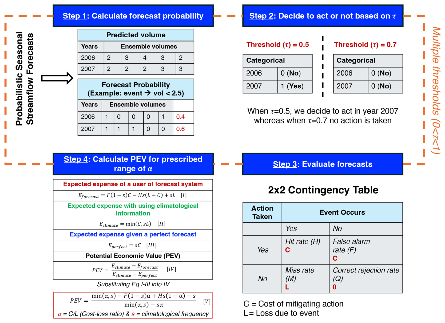
Figure 1 Flowchart showing the workflow to quantify the PEV using the probabilistic forecasts. For the calculation of PEV, forecast probabilities (for a given event) are calculated from the forecasts (Step 1), a critical probability threshold (τ) is applied (Step 2), a contingency table is created (Step 3), and, lastly, the PEV is calculated across the prescribed range of α (Step 4). The PEV relies on contingency table parameters (H and F), climatological frequency (s), and cost–loss ratio (α). The equations were adapted from Richardson (2000) and Jolliffe and Stephenson (2003).

Figure 2 illustrates an economic value diagram that depicts a PEV_max curve. This diagram visually represents the cost–loss ratio (α), on the x axis, whereas PEV is on the y axis. At low values of α, where the cost of preventive action is small relative to the potential loss, forecast systems tend to show higher economic value, as decision-makers can take advantage of accurate predictions to reduce potential losses with minimal expenditure. However, as α increases and the cost of preventive action becomes comparable to or exceeds the potential loss, the economic value of the forecast may decrease. In such cases, acting on the forecast becomes less advantageous because the cost of the preventive measure outweighs the potential benefit. The optimal economic value occurs when α is balanced in a way that maximizes the benefit of acting on the forecast while minimizing unnecessary costs. This usually happens when α is equal to the observed probability of the event (climatological frequency, s; Jolliffe and Stephenson, 2003). A value diagram, as shown in Fig. 2, will help decision-makers visualize and select appropriate actions based on their specific α (x axis) and the performance of the forecast system, compared with using climatology to determine the PEV (y axis). In Fig. 2, on the x axis, α=0 indicates that the cost of mitigation (C) is zero i.e., always beneficial, whereas α=1 indicates that the cost of mitigation (C) equals the potential loss (e.g., a farmer paying USD 10 000 as insurance money to prevent a loss of USD 10 000 due to a future event). PEV = 1 means that forecast-based decisions perform as well as those made using perfect information, while PEV = 0 indicates that the forecast offers no advantage over the baseline. A value of PEV = 0.7 at a given α suggests a 70 % improvement in decision-making, compared with using the climatology. Negative PEV values (gray boxes in Fig. 2) indicate decisions that would be worse than using the climatology (Laugesen et al., 2023; Richardson, 2000; Wilks, 2001).

To represent the forecast value in this study, we calculated the area under the PEV_max curve (now “APEV_max”) using the trapezoidal rule (Amlung et al., 2015). This method approximates the area by dividing the curve into trapezoids and integrating their areas. While negative PEV_max values are possible, they are excluded from the area calculation. Note that the PEV framework is applied iteratively across a range of critical probability thresholds ($\mathrm{0}<\mathit{\tau }<\mathrm{1}$) to identify PEV_max and to compute APEV_max by integrating over the corresponding curve. The resulting metric can be used as the “forecast value of a given forecast system” for the maximum economic benefits across all α (shown by the red shading in Fig. 2). A larger APEV_max curve indicates that the forecast system delivers higher economic value over a broad range of decision-making scenarios, regardless of α. This value ranges from 0, representing the theoretical minimum economic value, to 0.9, representing the highest overall economic value in this study, as negative PEV_max values are excluded from the area calculation.

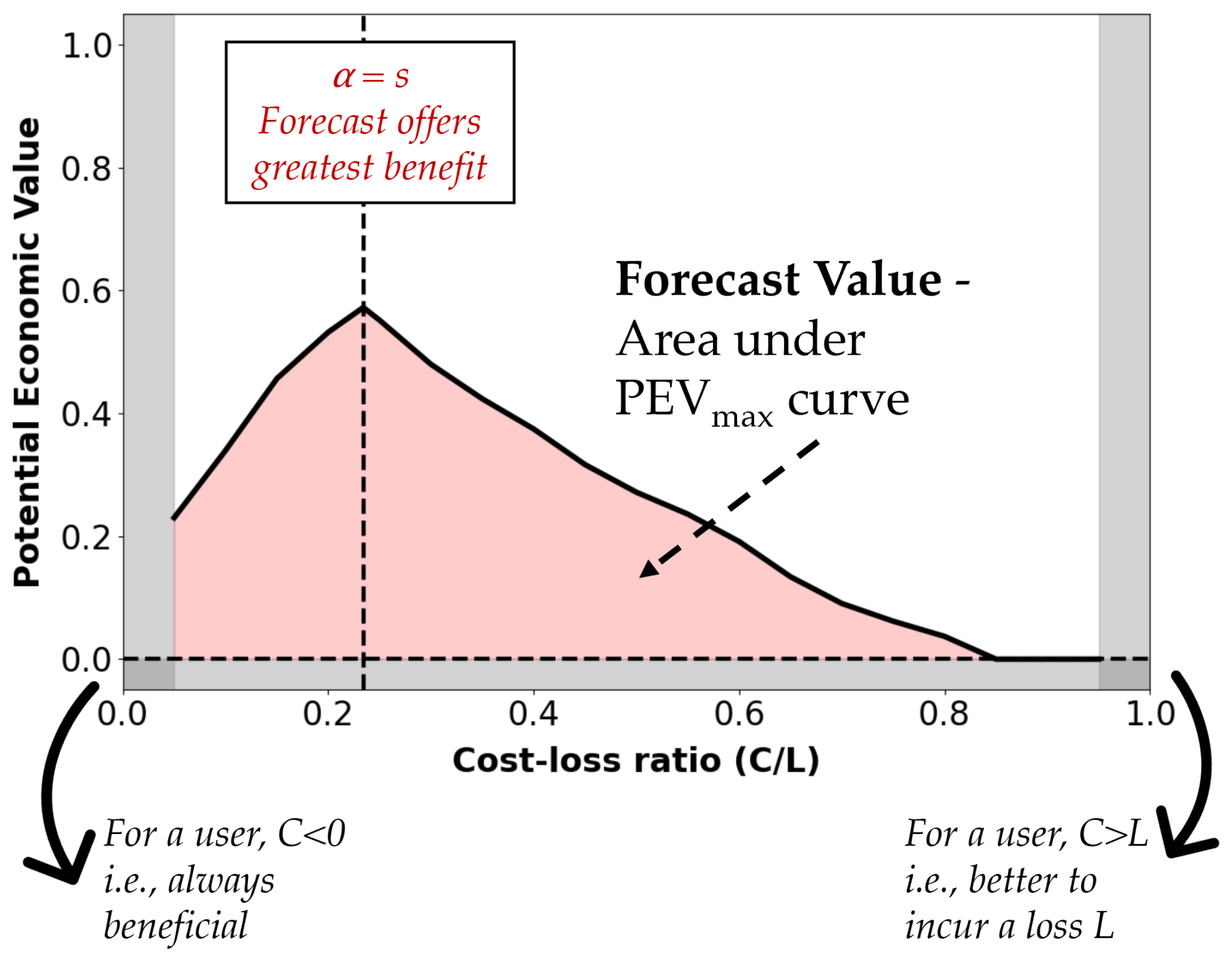
Figure 2 Economic value diagram showing cost–loss ratio (α) on the x axis and potential economic value on the y axis. The red shading shows the area under PEV_max (APEV_max). It highlights the positive PEV values across α, indicating that the forecast is preferred over climatology, whereas the gray regions highlight negative PEV values, indicating that climatology should be preferred. The left vertical gray boxes indicate that the user is always benefited when the preventive cost (C) is less than zero. In contrast, on the right, when the preventive cost (C) exceeds the potential loss (L), the user will always incur the loss L.

2.2 Study domain and basin screening procedure

Water availability in basins that are both unmanaged and snow-dominated is of interest here. These are often headwater catchments, with flows heavily driven by snowmelt timing and volume, making accurate forecasts essential for managing water resources and mitigating drought risks. Assessing forecast value in such basins is crucial since they often supply flows to downstream managed systems. We selected a diverse sample of drainage basins across the western US, representing a broad spectrum of hydroclimatic conditions. These basins were identified using geospatial attributes from three key sources: the USGS Geospatial Attributes of Gages for Evaluating Streamflow (GAGES-II) dataset, the Hydro-Climatic Data Network (HCDN; Slack and Landwehr, 1992), and the Catchment Attributes and Meteorology for Large-sample Studies (CAMELS) dataset (Addor et al., 2017; Newman et al., 2015). The basin screening procedure employed here was based on a similar approach to the CAMELS methodology (Addor et al., 2017; Newman et al., 2015) but with a slightly broader inclusion of basins from the GAGES-II dataset. Both the CAMELS basins and the additional basins included in our analysis are subsets of the GAGES-II dataset. As a result, most of the basins are unmanaged basins with drainage areas smaller than 2500 km², with minimal anthropogenic influence and at least 30 years of streamflow observations to ensure records for model training/calibration and validation.

Additional screening criteria were applied to the additional basins sourced from GAGES-II. These included limiting basins to those with not more than one major dam (defined as storage >5000 acre-feet (>6 167 400 m³)), ensuring that the ratio of reservoir storage to average streamflow (1971–2000) was below 10 %, and selecting basins with a GAGES-II hydrodisturbance index of less than 10 (Falcone et al., 2010). To further verify the accuracy of basin boundaries and drainage areas, we enforced additional criteria, based on GAGES-II boundary attributes. These included a boundary confidence score (on a scale of 2–10, with 10 indicating high confidence) of at least 8, a percentage area difference of not more than 10 %, compared with the USGS’s National Water Information System (NWIS) values, and a qualitative check to ensure that the HUC10 boundaries were deemed at least “reasonable” or “good” (further described in Falcone et al., 2010; Falcone, 2011). It should be noted that only 76 basins (out of 664 basins used for model training as described in Sect. 2.3.3) had NRCS forecasts available for the purpose of comparison. A majority of these basins lie within the US Environmental Protection Agency's level III snow ecoregions, labeled in Fig. 3. These basins are colored by the ratio of 1 April snow water equivalent (SWE) to water-year-to-date cumulative precipitation, which refers to the accumulated precipitation from the beginning of the current water year, 1 October, to 1 April, derived from gridded snow and meteorological forcings (as described in Table A2).

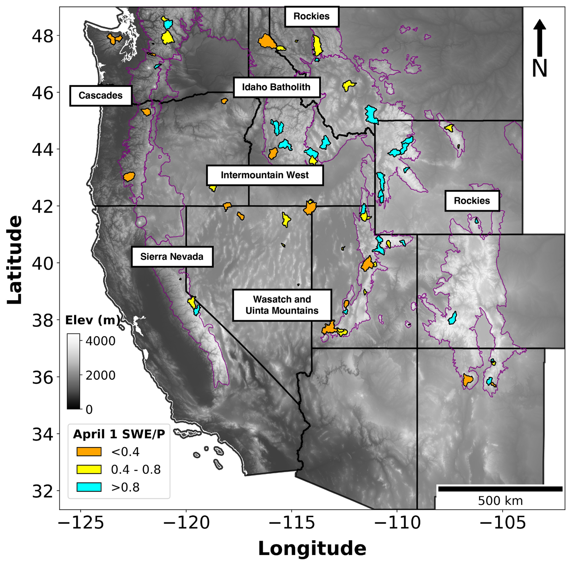
Figure 3 Study domain, comprising 76 USGS drainage basins across the western US, colored by the ratio of 1 April SWE to water-year-to-date precipitation. Purple boundaries indicate North American level III snow ecoregions generated by the US Environmental Protection Agency (US EPA, 2015). These ecoregions include the Cascades, Idaho Batholith, Intermountain West, Rockies, Sierra Nevada, and Wasatch and Uinta Mountains.

2.3 Synthetic forecasts

Synthetic forecasts are used to understand the impact of forecast-errors on economic value (Rougé et al., 2023) more clearly. We recognize that true forecasts have irregular error structures, which are difficult to interpret. To help interpret the relationship between forecast-errors and PEV in true forecast systems, we introduce systematic modifications to both the mean (error in mean) and standard deviation (change in variability) of observed AMJJ volumes (Gneiting et al., 2007). It should be noted that the change in standard deviation here is assumed to be with respect to the interannual variability seen in the observations, based on the retrospective years available in the forecast system. We generate the forecasts for the years WY2006–2022, where “WY” represents the water year, 1 October–30 September (Fig. 4). The choice to set the mean of synthetic forecasts equal to observations and the standard deviation to interannual variability ensures that the synthetic forecasts reflect key characteristics of the observed system. Aligning the mean with observations maintains comparability, while using interannual variability captures the system's inherent uncertainty. This design is crucial for studying irregular error structures, as it realistically represents the scale and variability of true forecasts. By mirroring these properties, the synthetic experiments provide a controlled yet representative framework for analyzing how irregular error structures impact forecast value.

The observations are modified by applying a percentage change to the mean, followed by a percentage change to the standard deviation (Fig. 4a). An ensemble of 39 forecast members (explained further in Sect. 2.4) is then generated, normally distributed around the modified mean and standard deviation. The varying spread of ensemble members reflects different potential hydrologic futures, allowing us to assess the performance of the forecast systems, not only in terms of a single prediction but across a wide range of possible outcomes. Additionally, if the errors result in negative values, we truncate the range of the forecast to be greater than or equal to 0, to avoid negative forecasts. In Fig. 4b, two synthetic forecasts are presented: one with a 50 % increase in both the mean and standard deviation, represented by the blue line and ribbon, and another with a 50 % decrease, represented by the red line and ribbon. These lines illustrate the ensemble spread of possible synthetic forecasts, based on the modified statistics. For comparison, the black dotted line and ribbon show the ensemble spread derived from the original observations and their standard deviation (i.e., interannual variability), serving as a reference point for evaluating deviations in the forecasts. Additionally, the white circle and triangle denote the original mean and standard deviation of the observations, respectively, offering a baseline to assess how the synthetic adjustments impact the overall distribution.

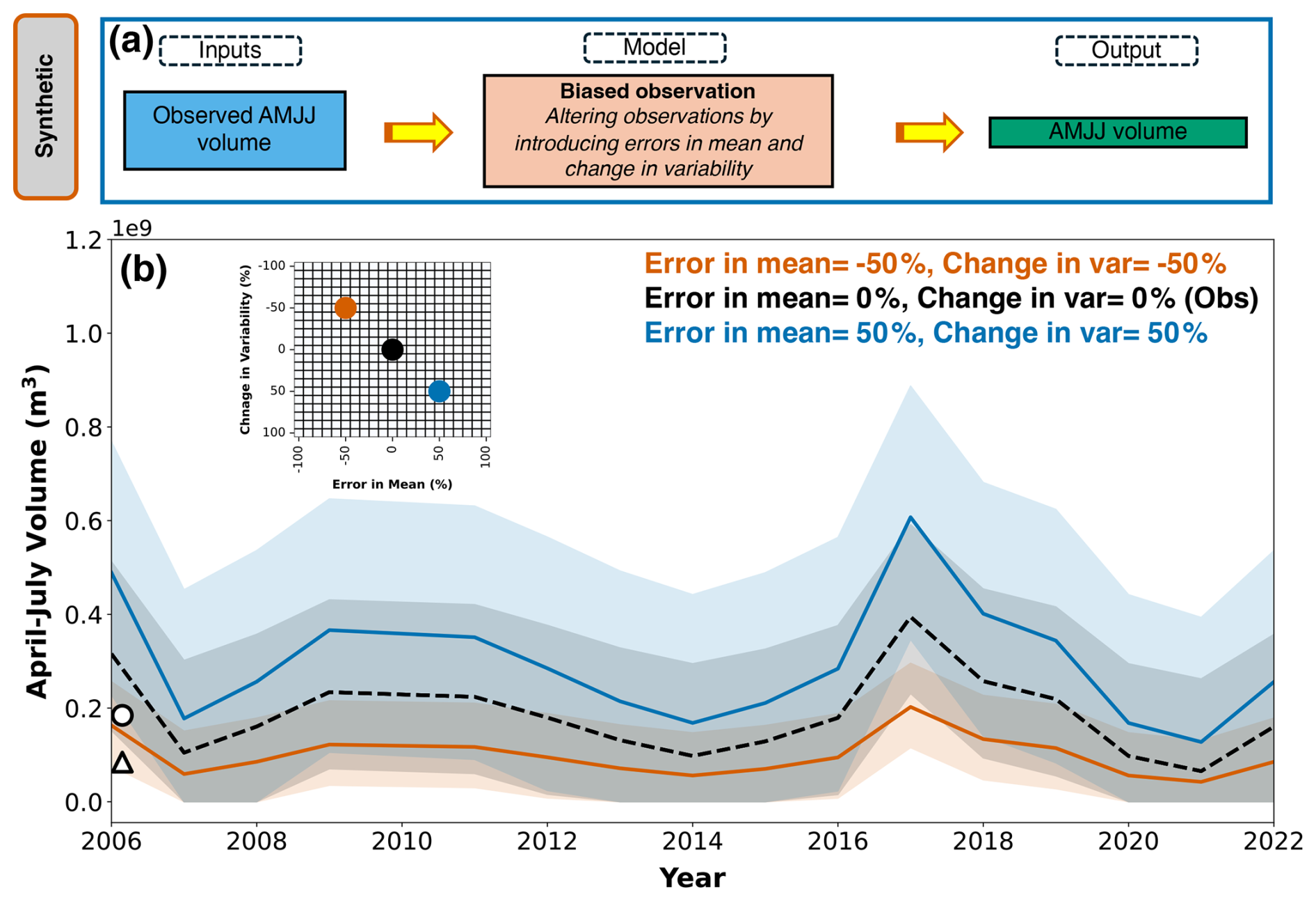
Figure 4 (a) The model workflow used to generate synthetic forecasts. (b) Two synthetic forecasts with ensemble spread in AMJJ volumes: one with a 50 % increase in both the mean and standard deviation, represented by the blue line and ribbon, and another with a 50 % decrease, represented by the red line and ribbon. The black dotted line and ribbon show the ensemble spread derived from the original observations and their standard deviation (i.e., interannual variability), whereas the white circle and triangle show the original mean and standard deviation of the observations, respectively. These forecasts correspond to different error structures, as shown in the inset grid.

2.4 True forecasts

A schematic of model workflows of three true forecast systems is provided in Fig. 5 – two designed for this study and one used operationally. The two designed true forecast systems use the ensemble streamflow prediction (ESP) framework. The first is a process-based hydrologic model (WRF-Hydro – WRFH; Gochis et al., 2020), which simulates streamflow evolution based on physical processes like snowmelt, soil moisture, and runoff (Fig. 5a). The second is a deep-learning model (LSTM; Hochreiter and Schmidhuber, 1997), which leverages historical patterns from the data (Fig. 5b). In these systems, the primary input data consist of historical meteorology, geospatial basin attributes, snowpack information in the form of SWE (only for the LSTM model), and streamflow observations, which are also used for training and validation (Table A2). It is important to note that WRFH is run on an hourly timescale and its outputs are aggregated into AMJJ volumes. Similarly, the LSTM model follows the WRFH approach but runs on a daily timescale, with its outputs aggregated into AMJJ volumes. A detailed description of the ESP methodology is provided in Sect. 2.4.1, and the implementation of the models, including input data, model architecture, calibration/training, and forecast generation, is discussed in Sects. 2.4.2 and 2.4.3.

In addition, we used NRCS operational forecasts over the study watersheds to benchmark true forecasts. These forecasts were chosen since they are methodologically consistent across all study regions and easily accessible for a larger number of basins and years. The NRCS employs a principal component regression model. This model is usually modified to retain the principal components (Garen, 1992; Lehner et al., 2017) and uses predictors like SWE, accumulated precipitation from SNOTEL, and antecedent streamflow from USGS to predict AMJJ volumes (Fig. 5c).

All true forecasts have the same number of ensemble members; five forecast exceedance probabilities, computed at 90 %, 70 %, 50 %, 30 %, and 10 %, are extracted. To clarify, 90 % means that there is a 90 % chance that the observed AMJJ volumes will exceed this forecast value and a 10 % chance that it will be less than this forecast value. These probabilities are based on the multiple ensemble members in all true forecasts. In order to make all forecasts comparable, the same five probabilities of exceedance were obtained from both true and synthetic forecasts. True forecast systems often deviate from idealized assumptions, exhibiting non-normal error distributions and varying variances, due to the influence of dynamic unpredictable factors and system-specific behaviors. This phenomenon is demonstrated in Fig. A3, where an exposition of these irregular error structures is presented through time-series analyses of AMJJ volumes. These time series illustrate how interannual fluctuations in volumes reveal underlying heteroscedasticity, skewness, and other deviations from standard statistical norms.

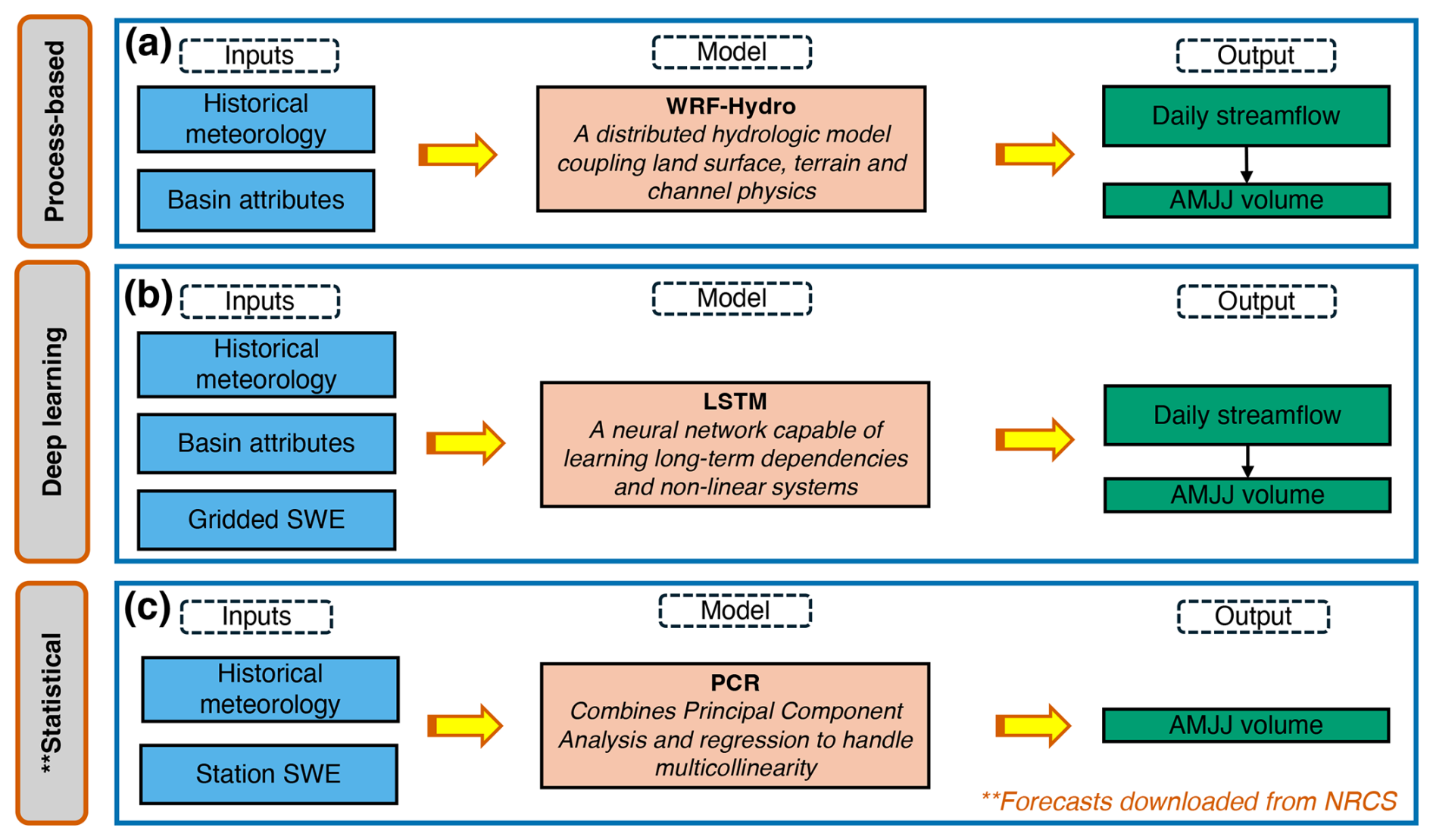
Figure 5 Model workflows used to generate true forecasts, including inputs, model type, and outputs: (a) process-based hydrologic model, WRF-Hydro; (b) deep-learning model, LSTM; (c) NRCS statistical forecasts.

2.4.1 Ensemble streamflow predictions (ESPs)

In general, ESP forecasts generated on 1 April (i.e., 1 April is the forecast date) hold significant operational importance. This is because 1 April historically serves as a surrogate for the timing of peak SWE conditions and provides near-maximum predictive information (Livneh and Badger, 2020; Pagano et al., 2004). In this study, 1 April, as a forecast date, is closely tied to forecast skill and serves as an optimal point for calculating forecast value. However, depending on the region and the context of decision-making, users may choose a different forecast date that better aligns with their needs and associated forecast skill. The ESP simulation begins at the start of the water year (1 October), utilizing true meteorological forcings to initialize the model's initial conditions on 1 April. Using these initial conditions on 1 April and meteorological forcings from previous years, an ensemble of streamflow traces is produced in the forecast period (April–July) as a function of the current hydroclimatic state and historical weather conditions (Day, 1985; Troin et al., 2021).

The result is a daily probabilistic hydrologic forecast, ranging from 30 d up to 180 d from the forecast date, that uses the spread in historical data from the previous ≈20 to 30 years (shown in Fig. 6 – for illustration purposes, we only show 23 years here) as an analogue for the uncertainty in meteorological conditions after the forecast date. For example, a forecast generated on 1 April (illustrated in Fig. 6) uses observed meteorology up to that date, with the model's initial conditions preserved, and then generates streamflow traces based on meteorological forcings from previous years for the remainder of the forecast period.

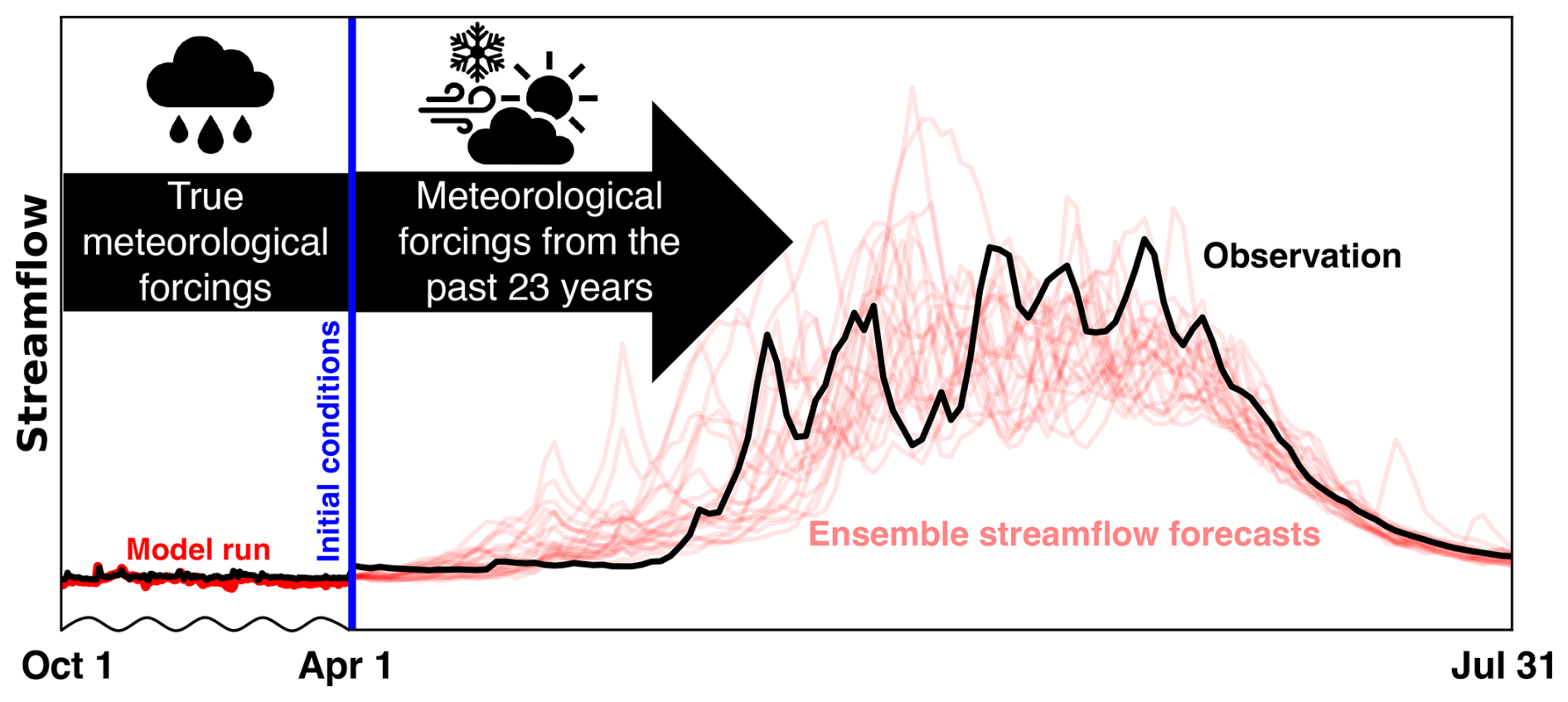
Figure 6 An ESP forecast issued on 1 April. The thick red line on the left depicts the model run before the forecast date using “true” meteorological forcings, starting from 1 October. Using the model's initial conditions on 1 April (shown in blue) and historical meteorological forcings from the past 23 years, ensemble streamflow forecasts are generated (shown with faint red lines). Data are from Johnson Creek, ID, USGS basin 13313000, for the forecast year 2011. The broken x axis shown here is not uniform and represents the ESP conceptually (Modi et al., 2024).

2.4.2 Implementation of WRF-Hydro in an ESP framework

WRFH model architecture

WRFH is a distributed hydrologic model architecture designed to facilitate the coupling of hydrologic models with atmospheric models through improved representations of terrestrial hydrologic processes associated with spatial redistribution of surface, sub-surface, and channel waters across the land surface (Gochis et al., 2020). As its modeling core, WRFH uses the Noah-MP land surface model, an improved version of the baseline Noah land surface model (Ek et al., 2003; Niu et al., 2011), which offers multi-parameterization through several vegetation, snow, radiation transfer, runoff, and groundwater schemes. We use the National Water Model (NWM) scheme configuration developed and managed by NOAA to generate short-to-medium-range streamflow forecasts over the 2.7 million stream locations nationwide (Cosgrove et al., 2024). We only match the physics permutations used in the NWM configuration and not the routing configuration used in the operational NWM. We rely on a channel network that uses a default channel structure and is generated using Hydrosheds Digital Elevation Model data (Lehner et al., 2008). WRFH is set up on a 1 km horizontal grid spacing, simulating lateral water redistribution on the surface and shallow sub-surface on a 100 m grid spacing. The model is run hourly, with model outputs aggregated daily for analysis purposes. A description of WRFH model parameters and calibration is provided in Sect. A1.

WRFH model inputs

Meteorological forcings used to run the WRF-Hydro (WRFH) include precipitation, average wind speed, 2 m average air temperature, incoming longwave and shortwave radiation, near-surface air pressure, and vapor pressure, obtained from the Analysis of Records for Calibration (AORC, Fall et al., 2023, as detailed in Table A2). The Noah-MP land surface model is parameterized using surface albedo, leaf area index, and green fraction from the Moderate Resolution Imaging Spectrometer (Myneni et al., 2015). Land-use/land-cover is obtained from the United States Department of Agriculture National Agricultural Statistics Service (George Mason University, 2019), soil type from State Soil Geographic (STATSGO), and maximum snow albedo and soil temperature from the WRF Preprocessing System data page managed by UCAR (WRF, 2019). Daily streamflow estimates from the USGS's National Water Information System (USGS NWIS) are obtained for the USGS stream gauges corresponding to the basin outlets, which are used to calibrate the model and are described in the following.

WRFH forecast generation

We generate WRFH ESP forecasts on 1 April for WY2006–2022 before (now WRFH_DEF) and after (now WRFH_CAL) calibration. These forecasts leverage historical meteorological data from all available years WY1983–WY2022 except the forecast year by using them as inputs to WRFH. For an ESP forecast on 1 April, the WRFH simulation begins at the start of the water year, i.e., 1 October, using true meteorological forcings to obtain WRFH's initial states (e.g., snowpack, soil moisture) on the forecast date. An ensemble of streamflow traces is produced in the forecast period using these memory states on the forecast date and historical meteorological forcings. The forecast daily streamflow is further cumulated to AMJJ volume and used for analysis.

2.4.3 Implementation of LSTM in an ESP framework

LSTM model architecture

This study adopts a model architecture similar to Kratzert et al. (2019), as followed by Modi et al. (2024) (now “M24”), which has been shown to simulate and forecast streamflow well for basins with minimal anthropogenic influence. This M24 setup only includes hyperparameters – externally set values that govern the training process – not model parameters or inputs. This list of hyperparameters is briefly outlined and explained in Table A3 (Sect. A2). Using the M24 setup, the LSTM includes a single hidden layer comprising 256 units, where units act as computational units through which data flow and the hidden layer is responsible for learning the intricate structures in the data. Additionally, the hidden layer is configured to randomly drop neurons during training, with a dropout rate of 0.4, to mitigate overfitting. The input sequence length used is 270 d, which specifies the number of preceding time steps fed into the LSTM to produce streamflow on a given day. A description of LSTM training is provided in Sect. A2.

LSTM model inputs

The training inputs for the LSTM model (as detailed in Table A2) include meteorological forcings from the AORC (Fall et al., 2023), which are aggregated daily and spatially averaged across each basin using 1 km grid cells and are identical to the WRFH inputs. These forcings consist of precipitation, average wind speed, 2 m average air temperature, incoming longwave and shortwave radiation, near-surface air pressure, and vapor pressure. In addition to these meteorological forcings, static predictors are included, consisting of basin attributes from the GAGES-II dataset, which remain constant over time and are selected to mirror those utilized in the CAMELS dataset, following the work of Arsenault et al. (2023) and Kratzert et al. (2019). We obtain daily snow information from the gridded snow dataset developed at the University of Arizona (now UA) (Broxton et al., 2019; Zeng et al., 2018), spatially averaged for each basin from $\mathrm{1}/\mathrm{16}$° grids. Lastly, daily streamflow estimates from the USGS's National Water Information System (USGS NWIS) are obtained for the USGS stream gauges corresponding to the basin outlets.

LSTM forecast generation

We generate LSTM ESP forecasts on 1 April for WY2006–2022, excluding years used in training, using model parameters from fully trained settings. These forecasts leverage historical meteorological data and snow information from all available years WY1983–WY2022 except the forecast year. For ESP forecasts on 1 April, the LSTM simulation begins at the start of the water year, i.e., 1 October, using true meteorological forcings and snowpack information to obtain LSTM's memory states on the forecast date. During the forecast period, the historical meteorological data are used similarly to process-based models. However, special treatment is applied to snowpack information, integrating known snowpack information for the forecast date and assumptions about snow evolution after the forecast date as a way to boost the representation of hydrologic memory that is commensurate with the physical hydrologic system. We adopt the “ESP_RetroSWE” forecast experiment from Modi et al. (2024), which integrates the known SWE information for the forecast date (from the forecast year) with explicit accumulation and ablation rates after the forecast data from individual historical years. More information on the design and performance of “ESP_RetroSWE” is provided by Modi et al. (2024). The forecast daily streamflow is further cumulated to AMJJ seasonal volumes and used for analysis.

2.5 Performance metrics

We employed four key performance metrics to compare the historical performance of our designed true forecast systems, drawing from those widely adopted to quantify streamflow accuracy. The Nash–Sutcliffe efficiency (NSE) was used to quantify streamflow prediction accuracy of the different models. The NSE ranges from −∞ to 1, with 1 indicating perfect agreement between the simulated and observed values and values closer to 0 indicating poorer performance. The normalized root mean square error (NRMSE, as a percentage) was used to analyze the skill of simulated AMJJ streamflow volume against the corresponding observed streamflow volumes. The RMSE was normalized by the median of observed streamflow volumes; values closer to 0 indicate better performance. The correlation assesses the agreement in patterns between the simulations and observations, with values ranging from −1 (perfect negative correlation) to 1 (perfect positive correlation). The ratio of standard deviation compares the spread between the simulations and observations to assess whether the simulations capture the correct level of variability in the observations. A ratio of standard deviation of 1 indicates that the simulations have captured the correct level of variability.

We use the relative median absolute deviation (RMAD) to compare the variability between synthetic and true forecasts. The RMAD measures the median of the relative absolute errors between the true and synthetic forecasts. Since both the true and synthetic forecasts are ensemble forecasts, the errors are calculated by first determining the absolute differences between corresponding ensemble members. These absolute errors are then normalized by the true forecast values to compute relative errors. The median of these relative errors across the ensemble members is then used to quantify the RMAD, with values closer to 0 indicating smaller deviations and better alignment between the true and synthetic forecasts. The metrics used to calibrate/train the true forecast systems are described in Sects. A1 and A2.

3 Results

We first compare the historical model performance from the WRFH and LSTM models with respect to the observations (Sect. 3.1). In Sect. 3.2, we analyze how error in mean and change in variability impact the forecast skill and value for synthetic (i.e., imposed errors on observations) and true forecasts (i.e., estimated with respect to the observations). In Sect. 3.3, we examine the relationship between forecast skill and value from different forecast systems, with different severities of drought and the impact of categorical variables, particularly on forecast value.

3.1 Historical model performance of our designed true forecast systems

We assess the performance of our designed true forecast systems using historical data to ensure their effectiveness in accurately simulating streamflow. We first compared the performance of the calibrated WRFH and fully trained LSTM models against observations for 76 basins during the testing period, WY2001–2010, using four key metrics: daily NSE, normalized root mean square error (NRMSE) of total AMJJ volume, daily correlation, and the ratio of the standard deviation (Fig. 7). The LSTM model consistently outperformed the WRFH model across all metrics, with statistically significant improvements. For example, LSTM showed a median NSE and NRMSE of 0.80 and 20 %, whereas WRFH showed 0.42 and 45 %, respectively. The median correlation was greater than 0.7 for both models, with LSTM showing the highest correlation, of 0.85, demonstrating a capability to capture temporal dynamics in daily streamflow prediction. LSTM also showed a reasonable ratio of standard deviation, of 0.95, whereas WRFH showed 1.25. These results suggest that the LSTM model performs much better in simulating streamflow than the WRFH model. The WRFH and LSTM showed satisfactory utility in simulating daily and seasonal streamflow and were chosen for further comparison to analyze the skill–value relationship for different model architectures. To underscore the importance of model calibration and training, we compare the performance of the models before and after calibration/training. In general, we observe improvements across all metrics for both models (additional details can be found in Sect. A3).

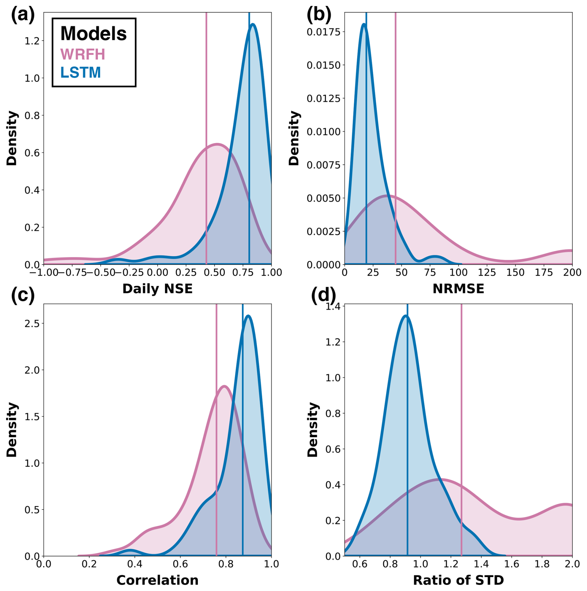
Figure 7 Historical model performance of true forecast systems: (a) daily NSE, (b) NRMSE of total April–July streamflow volumes, (c) daily correlation, (d) ratio of the standard deviation against observations for calibrated WRFH and fully trained LSTM models. Shaded areas represent the distributions of model performance metrics over the 76 basins, while vertical lines indicate the performance of individual basins during the testing period, WY2001–2010.

3.2 Forecast skill and value are affected by error in mean and change in variability

In Sect. 3.2.1, we first analyze synthetic forecasts to gain insights into their skill and value with respect to the error in mean and change in variability. In Sect. 3.2.2, we examine true forecasts, quantifying the error in mean and change in variability, and assess their skill and value (Sect. 3.2.2). Finally, we overlap skill and value from true forecasts with those from synthetic forecasts to diagnose and interpret how error in mean and change in variability impact forecast skill and value. We estimate skill and value only for the drought years (i.e., years below the 25th percentile based on observed AMJJ volumes between WY2006–2022).

3.2.1 Synthetic forecasts

Figure 8a and b illustrate the sensitivity of forecast skill and value to error in mean and change in variability across drought years. In Fig. 8a, a lower number indicates better forecast skill, meaning darker shades (close to purple) represent worse skill, whereas lighter shades (close to yellow) indicate good skill. The optimal forecast skill (close to zero) occurs particularly around errors in the mean between −20 % and 20 % and changes in variability of −100 % and −50 %. It is important to note that a standard deviation of 0 indicates that the forecast variability aligns closely with the historical interannual variability. As the error in the mean increases beyond these ranges, the forecast skill worsens. However, an increase in standard deviation reflects the variability of the probabilistic forecast, which is a characteristic of the forecast rather than a direct performance metric. In Fig. 8b, a higher number indicates a greater value, meaning that darker shades (close to purple) represent a low value, whereas lighter shades (close to yellow) indicate a greater value. The optimal forecast value (closer to 0.9) is observed with an error in the mean between −20 % and 20 % and a change in variability between −100 % and 0 %. A key observation is that a greater forecast value extends further into positive errors in the mean, compared with negative errors, resulting in a symmetric forecast skill around mean errors but an asymmetric forecast value.

We present four synthetic forecasts (Fig. 8c–f) to demonstrate how forecast skill and value are impacted by systematic error in mean and change in variability in the case of a categorical decision. In each plot, the black line and ribbon represent a synthetic forecast, with the mean equal to the observation and the standard deviation representing the interannual variability of the observations. The red dots indicate drought events, defined as AMJJ volumes below P₂₅. In Fig. 8c, with a −50 % change in variability, we can observe the highest skill (0.05) and value (0.62), as most events are correctly forecast (H=0.73), though a few ensemble members cause false alarms (F=0.06). In Fig. 8d, with a +50 % change in variability, all events are still hit (H=0.63) but the higher number of false alarms (F=0.20) reduces the forecast value from 0.62 to 0.42. Figure 8e, featuring a negative error in the mean, hits all events (H=0.87) but suffers from a high number of false alarms (F=0.70), resulting in a value of 0.03, while Fig. 8f, with a positive error in the mean, has almost no false alarms (F=0.01) but a lower hit rate (H=0.28), resulting in a value of 0.20. It should be noted that some ensemble members cause misses (M=0.13) and false alarm rates (F=0.01), as shown in Fig. 8e and f, respectively. This comparison reveals why forecast skill remains symmetric around the error in the mean, while forecast value is distinctly asymmetric. This asymmetry is largely due to the interplay of categorical measures, such as hit and false alarm rates, as well as our focus on events below the P₂₅ drought threshold. These factors lead to different sensitivities of skill and value to error in mean and change in variability.

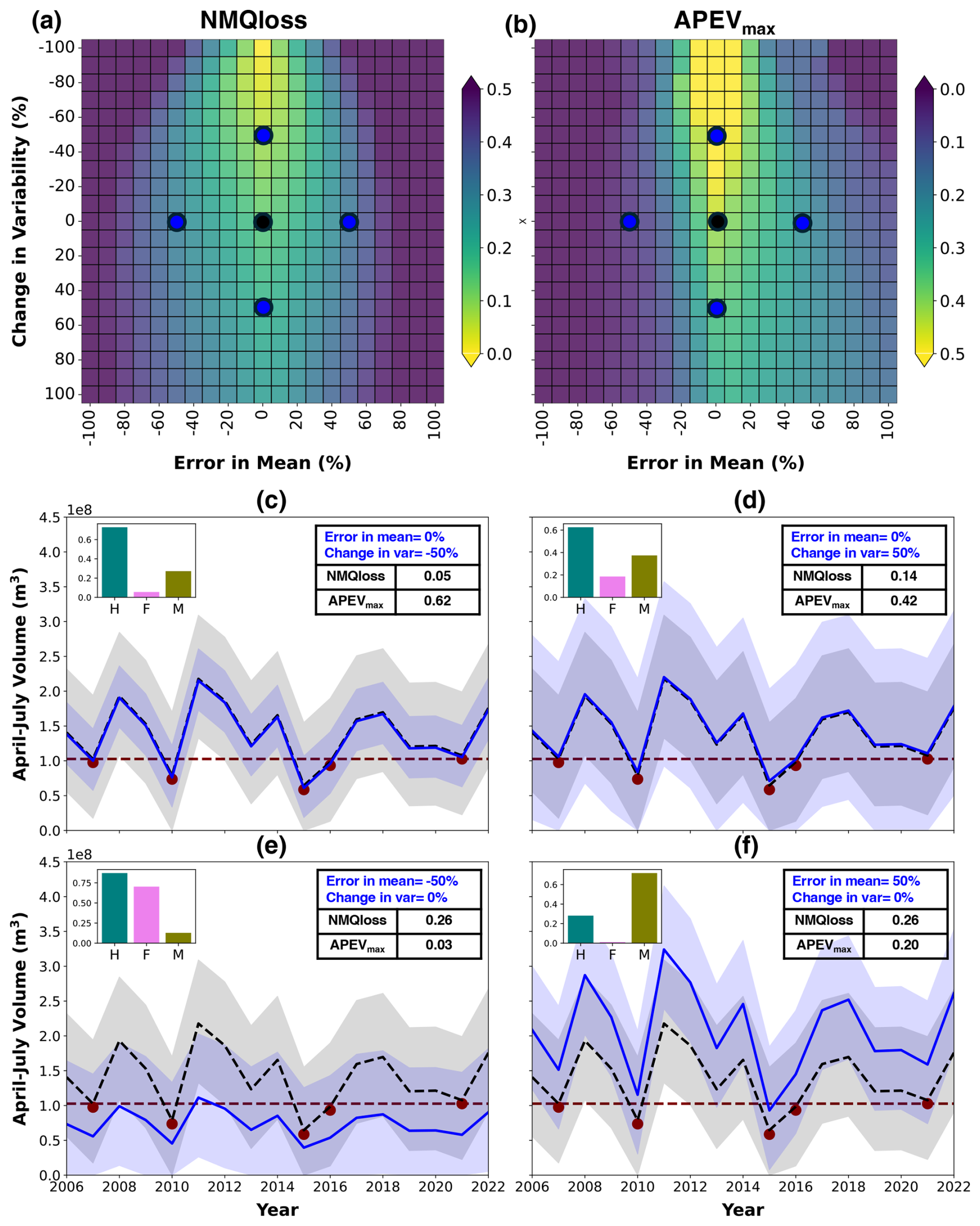
Figure 8 Sensitivity of quantile loss (forecast skill) and APEV_max (forecast value) to error in mean and change in variability for synthetic forecasts. (a, b) Background heatmaps represent synthetic forecasts, with (a) lower values showing better forecast skill (closer to yellow) and (b) higher values showing better forecast value (closer to yellow). (c–f) Four synthetic forecasts (shown in blue) corresponding to different errors in the mean and changes in variability. The black line and ribbon represent a synthetic forecast, with the mean equal to the observation and the standard deviation representing the interannual variability of the observations. The red dots indicate drought events, defined as AMJJ volumes below P_25, whereas the histograms represent the hit (H), false alarm (F), and miss (M) rates. Note that the color scale for forecast value is capped at 0.5, although the actual values reach up to 0.9.

3.2.2 True forecasts

Error in mean and change in variability

Figure 9 illustrates the error in mean and change in variability for all true forecast systems across 76 basins. Across all models, there is a consistent trend of overprediction in mean during drought years (Fig. 9a), with a standard deviation in forecasts lower than interannual variability from historical records (Fig. 9b). The degree of overprediction is generally higher in the Wasatch and Uinta Mountains and Rockies, while it is smaller in Sierra Nevada and the Cascades, Idaho Batholith, and Intermountain West. This is probably because the limited precipitation and snow observations in high-elevation regions introduce uncertainty in interpolated precipitation values (Vuille et al., 2018), which are assimilated into the model inputs (i.e., AORC). An intercomparison of the error in the mean across the models reveals significant differences. The median error in the mean is 55 % for WRFH, 30 % for the LSTM_, model, and 14 % for the NRCS model. The LSTM model shows lower mean errors than WRFH_CAL, aligning with historical performance trends, while the NRCS model performs best, exhibiting the smallest errors in the mean, as observed in Fig. 7. In contrast to overprediction of the mean, these models mostly show a standard deviation that is lower than interannual variability during WY2006–2022, as indicated by the decrease in standard deviation (Fig. 9b). These results are consistent with the trends observed in the synthetic forecasts (Fig. 8), where higher forecast skill and value were associated with a decrease in standard deviation. This understanding of the error in the mean and the change in variability underscores the importance of capturing both mean state and variability to improve forecast performance and value, particularly in complex mountainous regions like the Rockies, where observational limitations pose challenges.

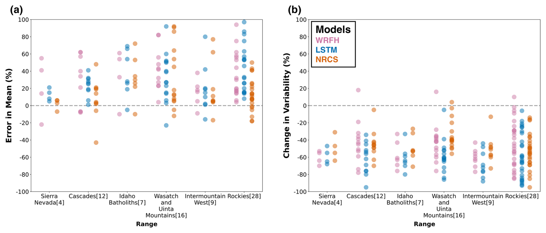
Figure 9 (a) Error in mean and (b) change in variability (with respect to interannual variability during WY2006–2022) of three true forecast systems (NRCS, WRFH, and LSTM). Each point represents a basin and the errors/changes are reported for drought years (below the P₂₅) between WY2006 and 2022. A total of 76 basins are divided across six ranges, with figures in square brackets representing the number of basins within each range.

Forecast skill

Figure 10 illustrates the normalized mean quantile loss (NMQloss) of the three true forecast systems over the heatmaps developed for synthetic forecasts, based on Fig. 8a. The background heatmaps represent the median skill from synthetic forecasts across basins, while the scatter points represent true forecast systems, based on the estimated errors with respect to the observation during drought years. Each dot in Fig. 10 represents a basin, with colors showing the median skill during drought years. We overlap true forecasts over synthetic forecasts to systematically analyze and understand the impact of irregular error structures in true forecast systems on the forecast skill. WRFH and the LSTM model show good correspondence, when compared with the synthetic forecasts (i.e., colors match well between the points and heatmap), based on the estimated RMADs of 30 % and 23 %, respectively. Notably, the NRCS model shows the highest consistency and robustness, with a RMAD of 20 %, closely aligning with the synthetic forecasts. The scatter points' distribution across each heatmap highlights the sensitivities of the forecast skill to error in mean and change in variability for the different forecast systems. Overall, this approach highlights the importance of considering error in mean and change in variability when diagnosing true forecast skill. It offers valuable insights into the reliability and robustness of forecasts in real-world scenarios, emphasizing how different systems perform under varying conditions of uncertainty.

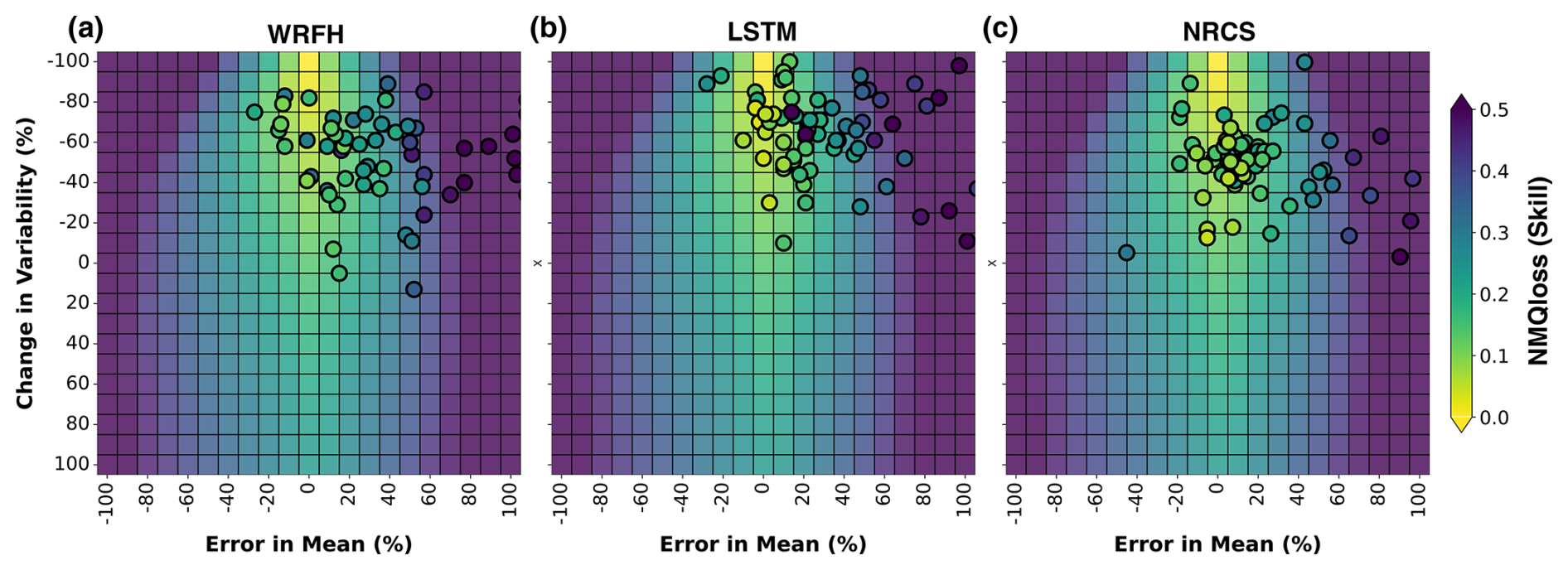
Figure 10 Comparison of skill between synthetic and true forecast systems for error in mean and change in variability. Normalized mean quantile loss (NMQloss) of three forecast systems (WRFH, LSTM, and NRCS) is represented as scatter points (each point represents a basin), indicating the true skill during drought years between WY2006 and WY2022. The background heatmaps represent the sensitivity of skill to error in mean and change in variability for synthetic forecasts. RMADs for true forecast systems from the optimal scenario are 30 %, 23 %, and 20 % for WRFH, LSTM, and NRCS, respectively.

Forecast value

Figure 11 is similar to Fig. 10; however, it focuses on APEV_max rather than NMQloss. Despite the good correspondence observed in forecast skill (Fig. 10), all true forecast systems demonstrate poor correspondence in value when compared with synthetic forecasts. This can be seen by the significant difference in the colors of points and heatmaps. This results in estimated RMADs for WRFH, LSTM, and NRCS of 100 %, 81 %, and 91 %, respectively, dramatically different from the deviations in skill. These large deviations show that the error in mean and change in variability do not effectively explain the variations in the forecast value between true and synthetic forecasts. None of the true forecast systems was able to consistently capture forecast value, as can be seen from our comparison with synthetic forecasts. The distribution of scatter points across each heatmap further emphasizes that APEV_max, unlike NMQloss, is not a simple function of the error in mean and change in variability or, in broad terms, forecast skill.

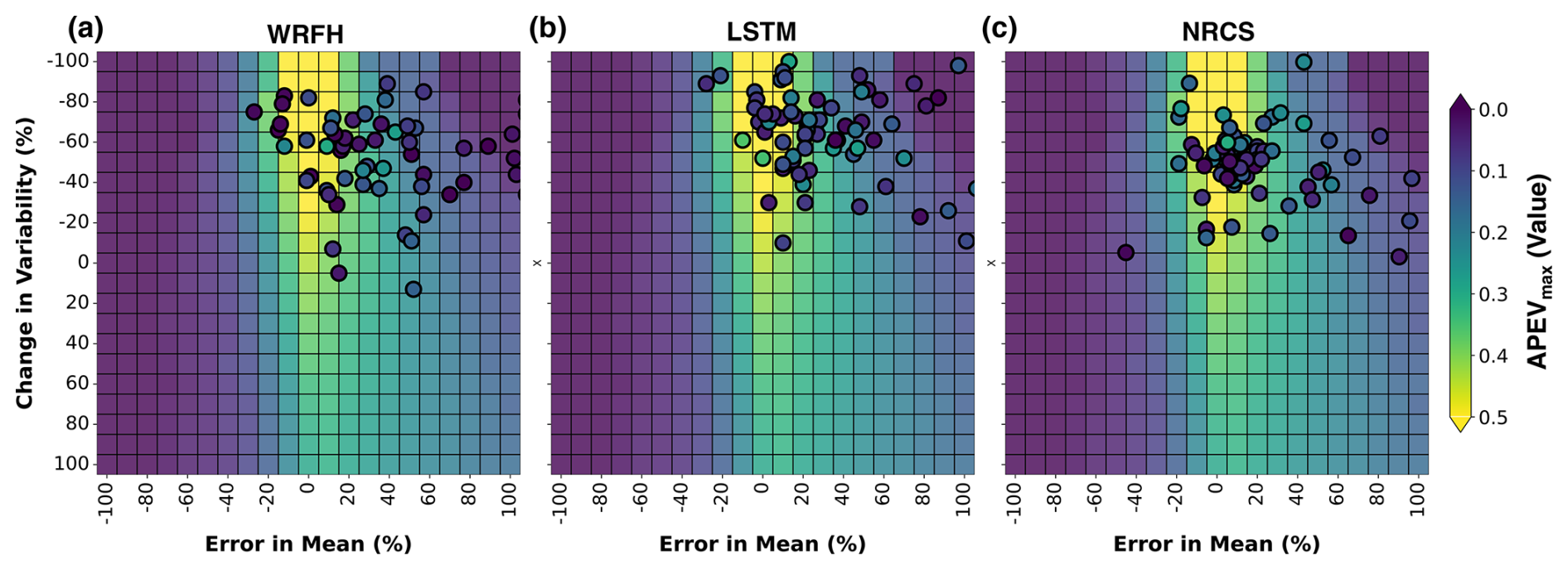
Figure 11 Comparison of value between synthetic and true forecast systems for error in mean and change in variability. Area under PEV_max curve (APEV_max) of three forecast systems (WRFH, LSTM, and NRCS) is represented as scatter points (each point represents a basin), indicating the true value during drought years between WY2006 and WY2022. The background heatmaps represent the sensitivity of APEV_max to error in mean and change in variability for synthetic forecasts. RMADs for true forecast systems from the optimal scenario are 100 %, 81 %, and 91 % for WRFH, LSTM, and NRCS, respectively.

3.3 Relationship between skill and value

3.3.1 Comparison between synthetic and true forecasts

We use the overlap between synthetic and true forecast systems from Figs. 10 and 11 to explore their skill–value relationship. Figure 12a compares the skill (NMQloss) and value (APEV_max) of the synthetic forecasts (i.e., grids in the heatmap) that overlapped with the true forecast systems (i.e., scatter points), based on error in mean and change in variability. Similarly, Fig. 12b shows the skill and value of the true forecast systems. Both scatter plots show the relationship between NMQloss (forecast skill) and APEV_max (forecast value) for the three true forecast systems (WRFH, LSTM, and NRCS), with each point corresponding to a different basin. The dashed lines in the plots represent fitted exponential curves, highlighting the general trend that, as skill increases (i.e., as NMQloss decreases), the value also improves (i.e., APEV_max increases). The optimal skill and value are obtained at the coordinates (0,1), where skill declines along the x axis and value increases along the y axis. For synthetic forecasts, this trend is more pronounced, with high correlation values (≥0.65) across all models, indicating a strong negative relationship between NMQloss and APEV_max across the entire range of NMQloss. In contrast, for the true forecasts, the relationship between NMQloss and APEV_max weakens (r≤0.38) and becomes more variable, suggesting that good forecast skill does not always translate to good forecast value (Turner et al., 2017). These plots collectively demonstrate that while NMQloss and APEV_max are related, their relationship is complex, particularly in true forecast systems. This skill–value comparison between synthetic and true forecast systems indicates that factors beyond forecast skill, as defined in this study, influence the value of true forecast systems, which we analyze in the following sections to some extent.

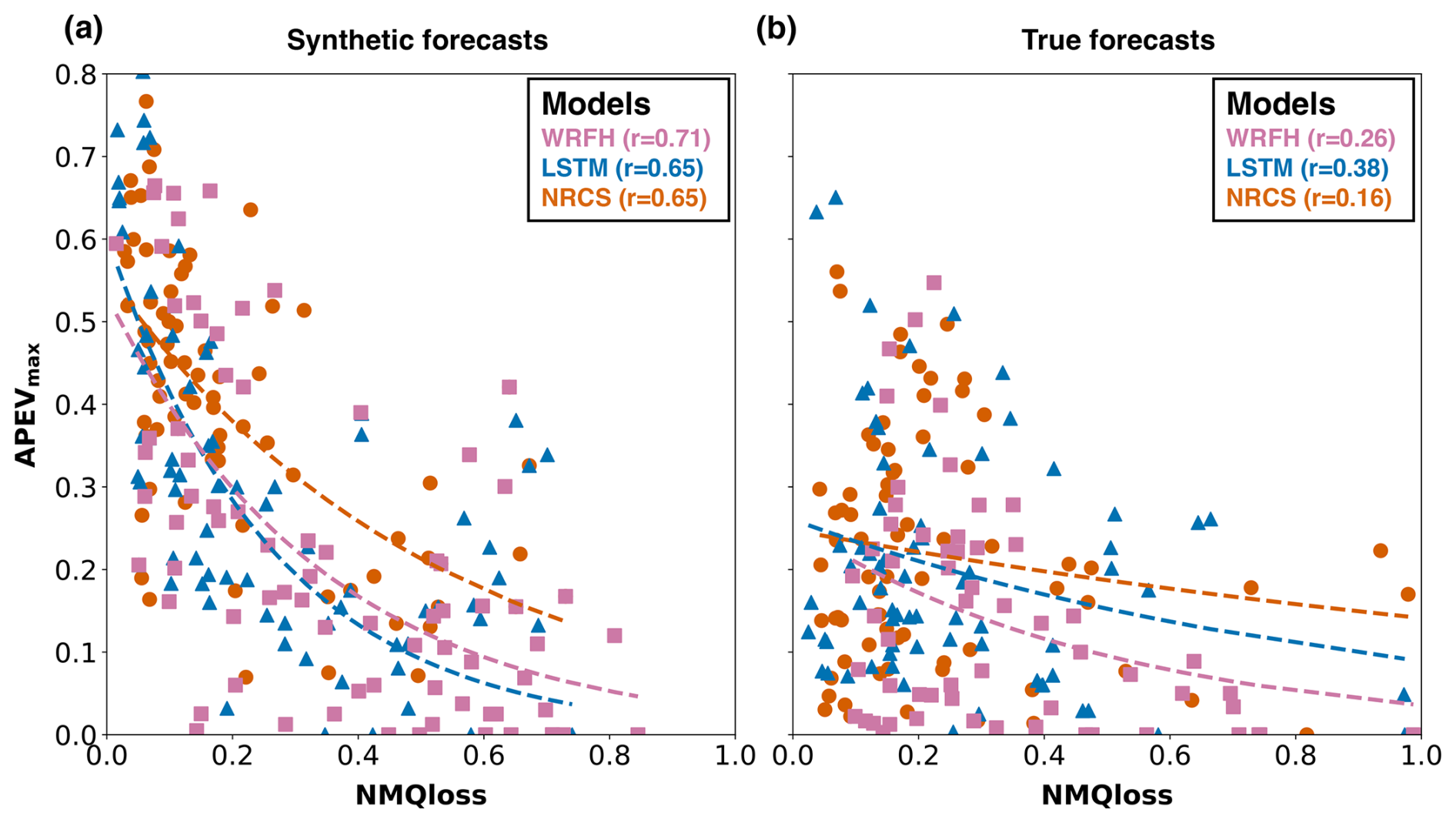
Figure 12 Scatter plots depicting the relationship between skill (NMQloss) and value (APEV_max) for synthetic and true forecast systems. The points in (a) and (b) represent the synthetic forecast (the grid of the heatmap) that overlap with true forecast systems (scatter points) in Figs. 10 and 11. Each point represents a basin, with the fitted exponential curves (dashed lines) indicating general trends and values in round brackets indicating correlation. It should be noted that we use the overlap from Figs. 10 and 11 to plot synthetic forecasts (corresponding to true forecasts) in Fig. 12a.

3.3.2 Skill–value relationship monotonically changes with the severity of drought

Figure 13 illustrates the relationship between NMQloss and APEV_max for three drought scenarios related to different severities. This includes three scenarios: AMJJ volume less than the 35th percentile (P₃₅), less than the 25th percentile (P₂₅ used consistently in earlier analyses), and less than the 15th percentile (P₁₅), represented by blue, orange, and magenta colors, respectively. Importantly, these scenarios are not independent of one another, as events identified below P₃₅ also encompass those below P₁₅ and P₂₅. The top density plot shows the distribution of NMQloss across all true forecast systems and basins, showing generally wide distributions with median values around 0.20. The right density plot represents APEV_max, which shows a consistent increase in median values from 0.12 to 0.20 as the drought severity decreases (i.e., from P₁₅ to P₃₅). This widening of distributions suggests that the estimated skill and value for drought scenarios that are not limited to extremely dry events (i.e., P₃₅) tend to improve, i.e., higher accuracy and better economic benefit. Hence, the relationship changes monotonically with drought severity. Therefore, the decrease in forecast value is likely to be attributable to the increase in forecast-error, as predictive models increasingly struggle in simulating progressively more extreme drought events (Chaney et al., 2015).

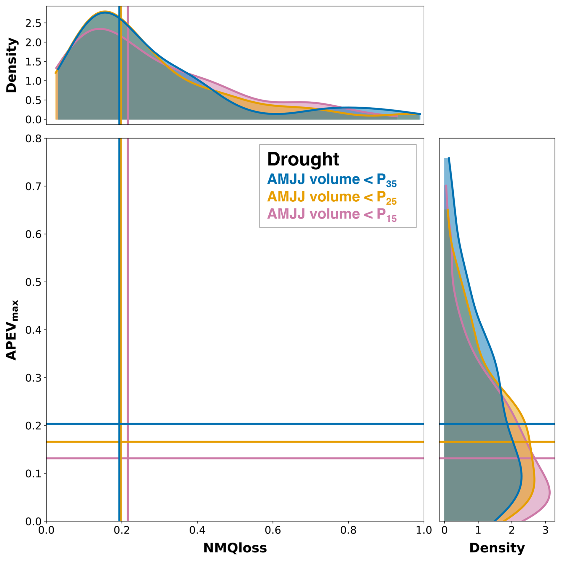
Figure 13 Relationship between NMQloss and APEV_max shown for three drought scenarios related to different severities. These drought severities are represented by AMJJ volume being less than 35th percentile (P₃₅, blue), 25th percentile (P₂₅, orange), and 15th percentile (P₁₅, magenta). The top density plot shows the distribution of NMQloss across all forecast systems and basins, whereas the right-side density plot displays the distribution of APEV_max.

3.3.3 Hit and false alarm rate and forecast value

In decision-making, a high hit rate ensures timely actions for critical events like drought, while a low false alarm rate limits unnecessary responses and maintains trust in the forecast system. Balancing these metrics is crucial for forecast value, as this determines the forecast's ability to support efficient and reliable decision-making. We analyze two critical components of APEV_max: the hit rate and false alarm rate (Fig. 14). This analysis focuses on two distinct basins, Dinwoody Creek, WY (Fig. 14a), and Lake Fork, CO (Fig. 14b), across various critical probability thresholds (τ) – the minimum probability at which a drought event is deemed likely enough to trigger an action. The left plots for each basin show the hit rate, while the right plots depict the false alarm rate. For this analysis, we compare the LSTM forecasts (shown in green) and the corresponding synthetic forecasts (shown in black), based on the overlap shown in Figs. 10 and 11.

In the case of Dinwoody Creek, both synthetic and true forecasts demonstrate a similar pattern, where, as the critical probability threshold (τ) decreases, the hit rate generally increases, eventually reaching a maximum of 1 (left panel of Fig. 14a). The value of 1 suggests that both forecasts effectively identify all drought events (below P₂₅ between WY2006 and WY2022) when the threshold becomes less strict. In terms of the false alarm rate, the synthetic forecast initially shows a lower rate compared with true forecast (LSTM), indicating fewer false alarms at higher thresholds (right panel of Fig. 14a). However, as the threshold decreases, the false alarm rates for both forecasts diverge significantly before converging at maximum rates of 0.5 and 0.75 for the synthetic and true forecasts, respectively. This divergence results in a notable difference in APEV_max values: 0.45 for the synthetic forecast and 0.08 for the true forecast.

In the case of Lake Fork, a similar trend is observed for the hit rate. As the critical probability threshold decreases, both the synthetic and true forecasts consistently detect more drought events as the threshold becomes less strict (left panel of Fig. 14b). However, the behavior of the false alarm rate differs from that in Dinwoody Creek. Here, both forecasts exhibit a gradual increase in the false alarm rate as the threshold decreases, but they converge more closely at maximum rates of 0.25 and 0.32 for the synthetic and true forecasts, respectively. This convergence results in similar APEV_max values for both forecasts, each approximately 0.42.

Overall, these analyses highlight how the balance between hit and false alarm rate impacts APEV_max in different basins. While Dinwoody Creek shows a clear discrepancy in economic value between synthetic and true forecasts due to their divergent false alarm rates, Lake Fork displays a more aligned relationship, with both forecasts yielding similar APEV_max values. These differences exist because of irregular error structures that are better captured in categorical measures than skill.

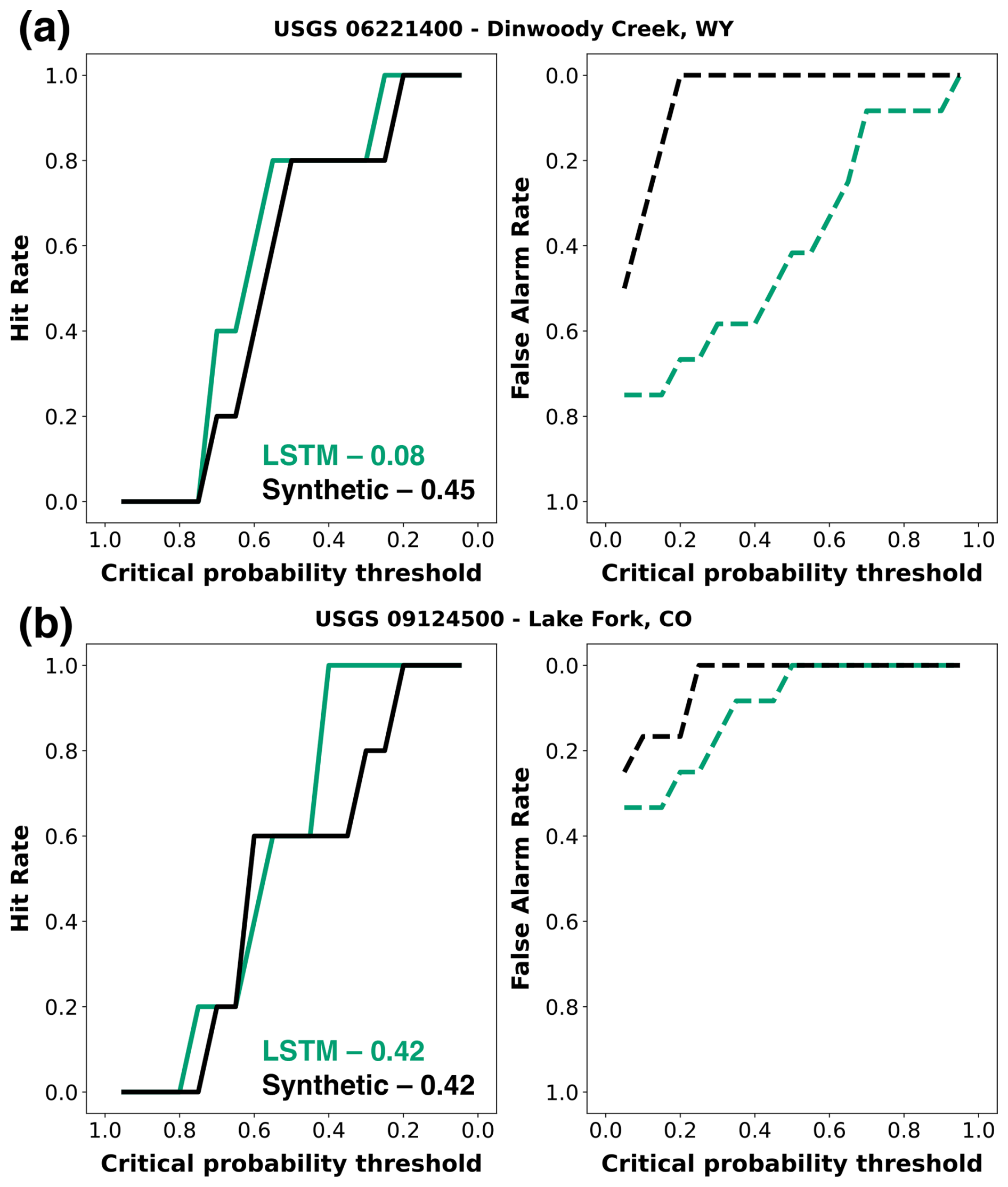
Figure 14 Attribution of hit rate and false alarm rate across varying critical probability thresholds (τ). Two basins are shown: Dinwoody Creek, WY (top panels), and Lake Fork, CO (bottom panels). The left panels show the hit rate as a function of the critical probability threshold (τ, minimum probability at which a drought event is deemed likely enough to trigger an action) for the LSTM forecast (green) and its corresponding synthetic forecast (black). The right panels depict the false alarm rate. The values indicate the APEV_max corresponding to each forecast system.

Figure 15 illustrates the forecast value of three true forecast systems with respect to hit and false alarm rates. Unlike Figs. 10 and 11, which analyzed error in mean and change in variability, this figure focuses on understanding the variability in the value with respect to hit and false alarm rates. The background heatmaps represent the median value from synthetic forecasts across basins, while the scatter points represent the median value from each forecast system. This comparison was performed across 76 basins during drought years (below P₂₅) between WY2006 and WY2022. Unlike Fig. 11, WRFH and LSTM show better correspondence of value when compared with the synthetic forecasts, based on the estimated RMADs of 78 % and 70 %, respectively. The estimated deviations are still higher, primarily resulting from differences in smaller magnitude of forecast value. Notably, NRCS shows the highest consistency and robustness, with a RMAD of 61 %, closely aligning with the synthetic forecasts.

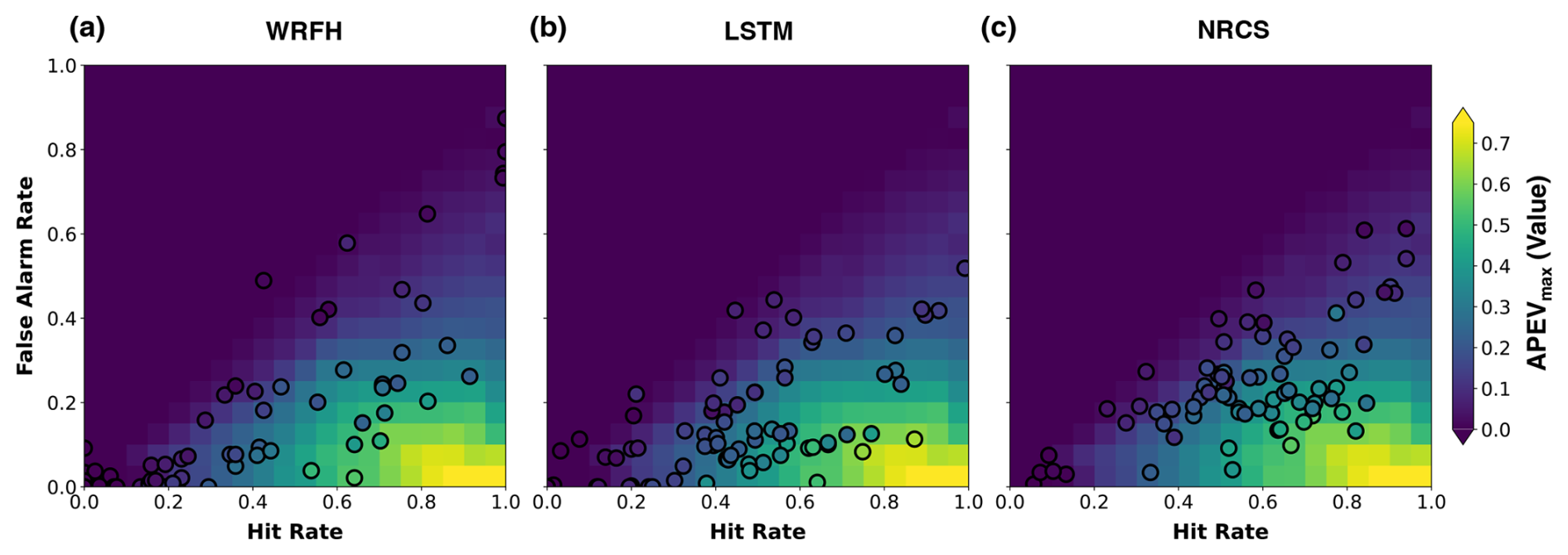
Figure 15 APEV_max of three forecast systems (WRFH, LSTM, and NRCS), represented as scatter points (each point represents a basin), indicating the actual value during drought years between WY2006 and WY2022. The background heatmaps represent the sensitivity of APEV_max to hit and false alarm rates for synthetic forecasts. RMADs for true forecast systems from the optimal scenario are 78 %, 70 %, and 61 % for WRFH, LSTM, and NRCS, respectively.

4 Discussion

We begin with a brief summary of our results, followed by a transition into a discussion of their broader implications. This study was motivated by recent literature showing that the relationship between forecast skill and value in hydrology is multi-faceted and context dependent (Giuliani et al., 2020; Hamlet et al., 2002; Maurer and Lettenmaier, 2004; Portele et al., 2021; Rheinheimer et al., 2016). While forecast skill generally reflects the accuracy of forecasts relative to observations, forecast value represents the economic benefits derived from utilizing those forecasts in decision-making. In this context, we emphasize that, while traditional accuracy metrics are fundamental for assessing forecasting systems, they have limited ability to capture the full utility of forecasts. By linking skill to value, we demonstrate how these metrics offer a more complementary perspective on forecast utility. We use the relatively simple PEV metric, based on a cost–loss model, to assess how forecast skill in 76 unmanaged snow-dominated basins translates into value, assuming a hypothetical group of decision-makers. Our analysis demonstrates that skill and value are not always aligned in a straightforward manner, attributed to the inherent quality of forecasting systems in unmanaged basins. To better understand the relationship between skill and value in the unmanaged basins from true forecasts, we compare these true forecasts with synthetic forecasts, created by imposing systematic errors on observed streamflow volumes (Fig. 4). Conversely, the true forecast systems include a process-based hydrologic model (WRF-Hydro), a deep-learning model (LSTM), and operational forecasts from the Natural Resources Conservation Service (NRCS).

We begin by assessing the historical model performance of true forecasts against observations generated in this study, comparing the WRFH and LSTM models across 76 basins using key performance metrics. As expected, the LSTM model consistently outperformed the WRFH model, probably due to the advanced capabilities of deep learning to better capture input–output dynamics (Fig. 7). We then analyzed the sensitivity of forecast skill and value to errors during drought years, specifically focusing on error in mean and change in variability. For synthetic forecasts, we expected that forecast skill would be symmetric around mean errors, while value would exhibit asymmetry due to the influence of categorical measures, such as hit and false alarm rates (Fig. 8). The use of a normally distributed ensemble to develop synthetic forecasts is a simplification that allows us to model forecast uncertainty in a controlled manner, while real-world forecasts often exhibit more complex, irregular, distributions and biases. For example, these may be overestimated in dry conditions and underestimated in wet conditions (Modi et al., 2022). A normal distribution was chosen to solely isolate the impact of mean and standard deviation. We recognize that this assumption does not fully capture the nuances of real-world forecast-errors, such as skewness or non-normality in extreme conditions, which would require detailed treatment outside the scope of this analysis. For the true forecast systems, we examined actual error in mean and variability against observations, observing a consistent pattern of overprediction in mean and variability lower than interannual variability from historical records (Fig. 9), as also reported in Modi et al. (2022). Additionally, we expected forecast skill for both synthetic and true forecasts to primarily follow patterns driven by error in mean and change in variability; indeed, the correspondence of forecast skill for both synthetic and true forecasts showed small differences, indicating that forecast skill was largely a function of error in mean and variability (Fig. 10). We acknowledge that estimating forecast skill and value for drought years necessitates a smaller sample size (here, n≈5), which is not ideal, affecting the statistical power of the analysis. This limitation arises due to the limited availability of operational forecasts and the need for sufficient ensemble members for ESP. Therefore, it would be important to assess whether a broader selection criterion or longer span of forecast availability would help ensure robust results.

However, we found three aspects particularly surprising. First, the skill–value relationship was remarkably consistent for synthetic forecasts, despite only controlling for mean and variability across the observations. This suggested that regular error structures allowed for a more predictable translation of skill to value (Fig. 12). Second, in contrast, the skill–value relationship was completely inconsistent for true forecasts, particularly in the context of droughts. This was unexpected; we had expected some level of variability, but the degree of inconsistency indicated that, in real-world conditions, forecast value is influenced by additional complexities beyond forecast skill (Fig. 12). Third, even though some true forecast systems, such as NRCS and LSTM, demonstrated high skill, the weaker skill–value relationship for true forecasts meant that good forecast skill did not always translate to high forecast value (Figs. 11 and 12).

Lastly, we found that categorical measures, such as the hit and false alarm rates, better explained the discrepancies in forecast value between synthetic and true forecast systems than the skill metric used in the study (Fig. 14). This was confirmed by showing the correspondence of forecast value between synthetic and true forecasts, which was largely driven by categorical measures like hit and false alarm rates (Fig. 15). Our findings highlight the risk of stakeholders relying solely on traditional performance metrics when selecting a forecasting system. While high forecast skill may indicate good performance, the economic value can vary significantly due to system complexities and interactions. This underscores the need for more sophisticated assessment approaches that consider forecast value, particularly in decision-making contexts, rather than focusing solely on skill metrics. Our study advocates for a multi-faceted assessment framework that integrates both skill and value while also recognizing the limitations of the PEV framework.

However, the PEV framework assumes risk-neutral decision-makers and is limited to binary decision contexts, which may oversimplify real-world decision-making challenges (Laugesen et al., 2023). In water management, decisions often involve continuous or multi-categorical variables, such as balancing water supply needs, hydropower generation, and flood control, which PEV does not fully capture (Laugesen et al., 2023; Portele et al., 2021). We also recognize that, while the PEV framework assumes equal costs for hits and false alarms, real-life decision-making may be more sensitive to false alarms, due to their potential to damage trust in forecasting systems and decision-making authorities. To better reflect decision-making contexts, it may be beneficial to explore weighted quantile loss metrics, where different quantiles receive different weights, depending on their relative importance in decision-making. Such a weighting scheme would better align with situations where high or low values have disproportionate consequences, as is often the case in hydrologic forecasting. While more advanced and flexible metrics, like the relative utility value (RUV; Laugesen et al., 2023), offer improved decision-making capabilities by incorporating user-specific utility functions, we opted for PEV due to its simplicity and broad operational applicability. RUV provides granular insights into forecast value across different decision thresholds but introduces additional complexities that are unique to individual users, including their decision-making preferences, risk tolerance, and operational priorities. RUV uses the same inputs as PEV. However, RUV allows the economic model, damage function, and risk aversion to be explicitly specified (Laugesen et al., 2023). One of the important benefits of RUV is that it uses the whole probabilistic forecast and does not need conversion to a categorical forecast, like PEV (Laugesen et al., 2023). PEV's straightforward interpretation and widespread usage in hydrologic and meteorological applications made it more suitable for our evaluation without introducing unnecessary complexities. The results from this study raise an important question about whether the categorical nature of the events and the experimental nature of PEV are indeed driving the observed outcomes. This potential alignment may suggest that categorical error measures are performing better, simply because they match the structure of our experimental design. To clarify this, further consideration is needed to understand whether this relationship reflects a true advantage of categorical measures or is an artifact of the setup, i.e., a comparison with the synthetic forecasts generated by imposing regular error structures. By testing alternative error measures like RUV that are not categorical and adjusting the experimental design, we can better assess whether the effectiveness of the forecasts is truly a function of forecast skill or simply due to the structure of the experiment. Such additional analysis will help confirm or refute the notion that categorical measures work better only because they align more closely with how events and costs are defined in this model. Future work could explore ways to incorporate asymmetric cost structures or impacts of reputation to better reflect these considerations in operational settings.

There are several limitations to the probabilistic forecasts used in this study. First, the datasets used for generating these forecasts typically have their own limitations, such as the absence of common standards for intercomparison, a lack of uncertainty estimates for assessing data reliability, and a lack of characterization of human intervention (Addor et al., 2020). In the case of LSTM ESP forecasts, the use of only a single deep-learning model (LSTM) is a limitation; this model could be replaced by alternative neural networks (Cho et al., 2014; Vaswani et al., 2017) or physics-guided architectures (Feng et al., 2022, 2023; Hoedt et al., 2021) to improve forecast performance. Additional limitations, as discussed by Modi et al. (2024), include the need to test different hyperparameters, extend the training period, and explore the use of other snowpack treatments that may improve the model's performance. For WRFH ESP forecasts, biases in initial hydrologic conditions, which arise due to lack of knowledge, incomplete process representation (DeChant and Moradkhani, 2011), and parameter uncertainty potentially resulting from ill-constrained calibration (Arheimer et al., 2020; Hirpa et al., 2015; Wood et al., 2016), contribute to forecast biases.

We also recognize that a comparison with operational ESP forecasts generated by the River Forecast Centers might be more appropriate for this study. However, due to the limited availability of operational ESP forecasts (starting in 2015) for our study basins, as well as inconsistent methodologies across regions, we chose to use the NRCS forecasts. Importantly, it should be noted that the differences in forecast volumes between NRCS and operational ESP forecasts are minor in the context of the overall forecast uncertainty (Lukas and Payton, 2020).

5 Conclusions

This study explored how the skill of seasonal streamflow forecasts translates to economic value for decision-making in unmanaged basins across the western US. We used synthetic forecasts to systematically analyze the skill and value of true forecasts produced by process-based (WRFH) and deep-learning (LSTM) models, as well as operational forecasts from the NRCS. The WRFH and LSTM models showed distinct responses to training and calibration in simulating streamflow. The LSTM model was more sensitive to training, with more stable structures, lower NRMSE, and better correlation. In contrast, the WRFH model showed minimal improvements post-calibration, with larger and more irregular error structures, despite some improvement in variability.

Our results showed that forecast skill – indicating how accurately forecasts match observations – and forecast value – representing the economic benefits derived from those forecasts in decision-making – exhibit complex relationships for true forecasts, due to their irregular error structures. Our comparisons between synthetic and true forecasts revealed that forecast skill across the basins was more sensitive to error in mean and change in variability than the forecast value. However, these errors do not adequately explain the variations in forecast value. This is primarily due to the irregular model error structures, which impact categorical measures, such as hit and false alarm rates, causing high forecast skill to not necessarily result in high forecast value. This suggests that overall model performance – how well a model handles variability and uncertainty – can significantly influence the gap between forecast skill and value. This gap is further complicated by the complexities introduced by operational structures.

The analysis also reveals a clear relationship between drought severity and skill–value relationship. Models consistently struggle to predict severe drought events, and forecast value worsens monotonically with drought severity. We conclude the study by demonstrating that categorical error measures, such as hit and false alarm rates, largely explained the forecast value. Our findings emphasize that forecast value is influenced by factors beyond forecast accuracy, such as the error structures and user-specific decision-making. This suggests that simple reliance on performance metrics can lead to important variations in economic value being overlooked. To address this, a more sophisticated evaluation approach is needed – one that prioritizes forecast value under varying conditions, rather than focusing exclusively on accuracy metrics. A comprehensive evaluation framework that integrates both skill and value is essential for more informed, impactful decision-making.

Appendix A

A1 WRFH model parameters and calibration

WRFH has several tunable parameters, associated with soil properties, surface and sub-surface routing schemes, baseflow and groundwater schemes, snow schemes, and the channel configuration (Cuntz et al., 2016; Lahmers et al., 2021). We use a calibration approach associated with the NWM scheme configuration, following Lahmers et al. (2021) and Cosgrove et al. (2024), that selects calibration parameters based on previous sensitivity studies (Cuntz et al., 2016; Mendoza et al., 2015), model developer surveys, and a WRF-Hydro parameter sensitivity study (further described in Lahmers et al., 2021). These parameters are distributed (distinct to each grid), and the calibration is performed by either using scalar multipliers (multiplying a scalar value from the calibration range with the actual values, as shown in Table A1) or simply replacing the actual values. The scalar multipliers ensure that the original model parameters are spatially coherent and physically consistent with a priori catchment properties (e.g., Gupta et al., 2008, 2009), whereas the replacement ensures that parameters are constant throughout the entire domain. The model parameters tuned for this analysis are mentioned in Table A1, including the calibration range, initial values, adjustment type, parameter description, and units.

Table A1 WRFH calibration parameters, including their calibration range, initial values, adjustment type, parameter description, and units.

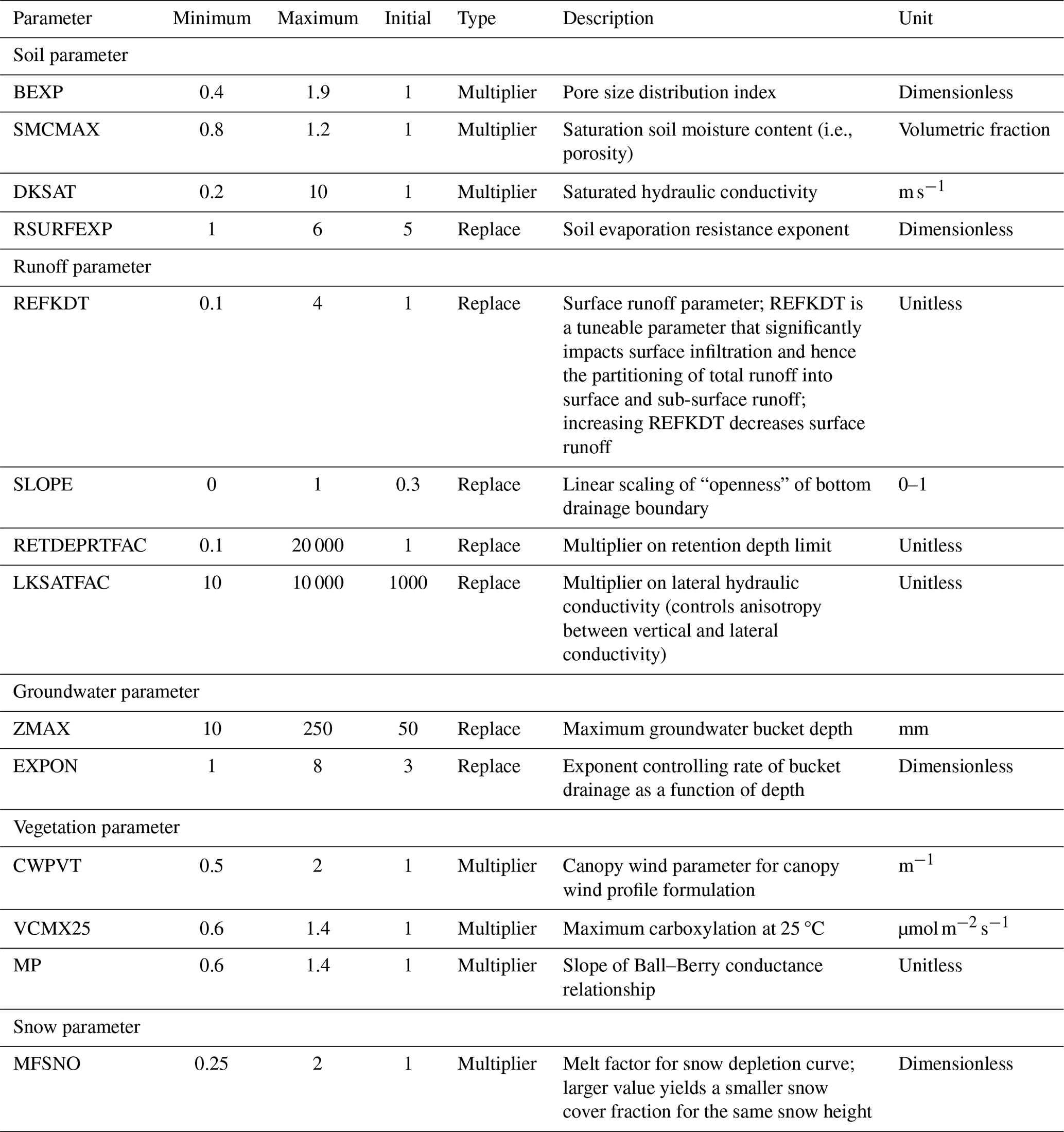
A total of 14 model parameters were calibrated with an iterative dynamically dimensioned search approach (Tolson and Shoemaker, 2007). This algorithm was developed for computationally expensive optimization problems, such as distributed watershed model calibration, and automatically scales the search strategy in model parameter space based on user-specified maximum iterations (Tolson and Shoemaker, 2007). In the initial iterations, the algorithm searches globally; as the procedure approaches the maximum number of iterations, the search transitions from a global to a local search, making it computationally efficient, and finds equally good solutions, compared with the dominant Shuffled Complex Evolution algorithm (Tolson and Shoemaker, 2007). In this study, the model is cycled over the calibration period 250 times to minimize an objective cost function, based on the works of Cosgrove et al. (2024) and Lahmers et al. (2021). It is important to note that we restrict the iterations to 250 due to limited computing resources. However, in an ideal scenario, such as an operational context, this number could scale up to thousands of iterations, depending on the complexity of the physical processes in the region. A 5-year calibration period for each basin was selected based on the maximum standard deviation of streamflow between WY1986 and WY2005. This ensures that calibration periods are selected based on, first, the basin's hydrologic conditions that are responsible for its water balance simulations and, second, the distinct climate years that allow for consideration of the broad effects of non-stationarity (Myers et al., 2021). A 5-year calibration period is short but has been adopted in earlier model implementations, owing to the limitations of computational resources (Cosgrove et al., 2024; Lahmers et al., 2021). The objective cost function is a weighted Nash–Sutcliffe efficiency (NSEwt),

$$\begin{array}{}\text{(A1)}& \begin{array}{rl}\text{NSEwt}={\displaystyle \frac{\mathrm{1}}{\mathrm{2}}}& \left(\mathrm{2}-{\displaystyle \frac{{\sum }_{t=\mathrm{1}}^T{\left(Q_{\mathrm{obs},t}-Q_{\mathrm{sim},t}\right)}^{\mathrm{2}}}{{\sum }_{t=\mathrm{1}}^T{\left(Q_{\mathrm{obs},t}-Q_{\mathrm{sim},t}\right)}^{\mathrm{2}}}}\right.\\ & \left.-{\displaystyle \frac{{\sum }_{t=\mathrm{1}}^T\left(\log \right(Q_{\mathrm{obs},t})-\log (Q_{\mathrm{sim},t}){)}^{\mathrm{2}}}{{\sum }_{t=\mathrm{1}}^T\left(\log \right(Q_{\mathrm{obs},t})-\log (Q_{\mathrm{sim},t}){)}^{\mathrm{2}}}}\right),\end{array}\end{array}$$

consisting, in equal parts, of NSE (Nash and Sutcliffe, 1970) and NSE calculated for the log of the discharge (NSE_log) using daily streamflow observations (Cosgrove et al., 2024; Lahmers et al., 2021).

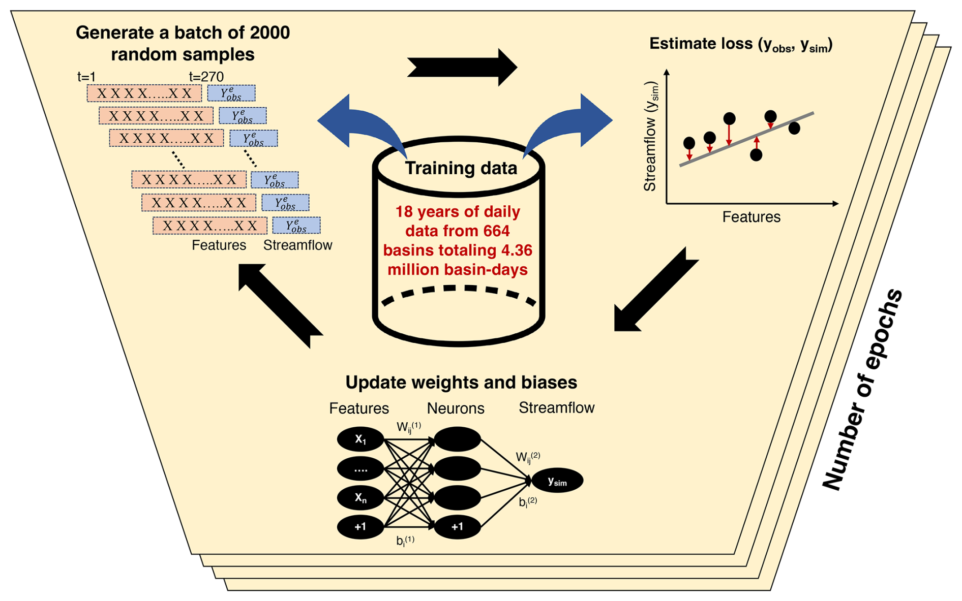
Figure A1 LSTM model training for each iteration within an epoch. In each iteration, 2000 independent random samples are drawn from 18 years of daily data from 664 basins totaling 4.36 million basin-days. Each sample consists of 270 d, i.e., input sequence length, of preceding predictors (X) and one target observation (y_obs). The loss is computed between observed discharge (y_obs) and the network's prediction (y_sim). Model parameters, including weights (w₁…w_m) and biases (b₁…b_m), are updated after every iteration. The term “epoch” refers to the complete passing of the entire training dataset through the model algorithm once. The weights and biases are model parameters, whereas the batch size, input sequence length, and number of epochs are the hyperparameters (Modi et al., 2024).

A2 LSTM model training

The LSTM training process, as illustrated in Fig. A1, was adapted from Modi et al. (2024), who provide a more comprehensive exposition. It begins by initializing weights and biases using the Xavier uniform distribution (Glorot and Bengio, 2010). During each iteration, a random batch of 2000 samples is drawn from the training data to make predictions. The model is trained regionally, using training data from 664 basins across the CONUS from WY1983 to WY2000. Each sample consists of a streamflow observation on a given day (the dependent variable) and the input sequence of the preceding 270 d, creating a “sequence-to-value” prediction. Since streamflow on any given day is dependent on the preceding 270 d, batches are randomly selected across basins without requiring chronological order (Kratzert et al., 2018). Static basin attributes alongside meteorological forcings are included as inputs to inform the model of basin characteristics. During each iteration, the predictors (X) pass through the model's weights (w) and biases (b) to produce streamflow predictions (y_sim), and the error (or loss) is computed relative to the observations (y_obs). The model parameters are then updated through back-propagation.

To account for varying hydroclimatic conditions across basins, the training loss function is a basin average Nash–Sutcliffe efficiency (NSE), which normalizes the mean squared error for each basin using streamflow variance (Kratzert et al., 2019). This prevents large humid basins from dominating the loss function. Unlike process-based models, where parameters are updated after each complete model run, LSTM parameters are updated after each epoch – where an epoch represents one full pass of the training data. For example, if there are 100 000 training samples and a batch size of 2000, one epoch would consist of 50 iterations (100 000/2000). In this study, 40 epochs were used for training with a single seed and the Adam optimizer, which offers better efficiency than stochastic gradient descent (Ruder, 2016). Multiple seeds were not tested, as the performance impact was minimal (Kratzert et al., 2019).

Table A2 Training predictors for LSTM models, consisting of meteorological forcings (source: AORC), static basin attributes (source: GAGES-II), and snow data (source: UA), with streamflow data (source: USGS) as the predictands. The asterisk indicates that the predictor was only included in one of the two trained LSTM models.

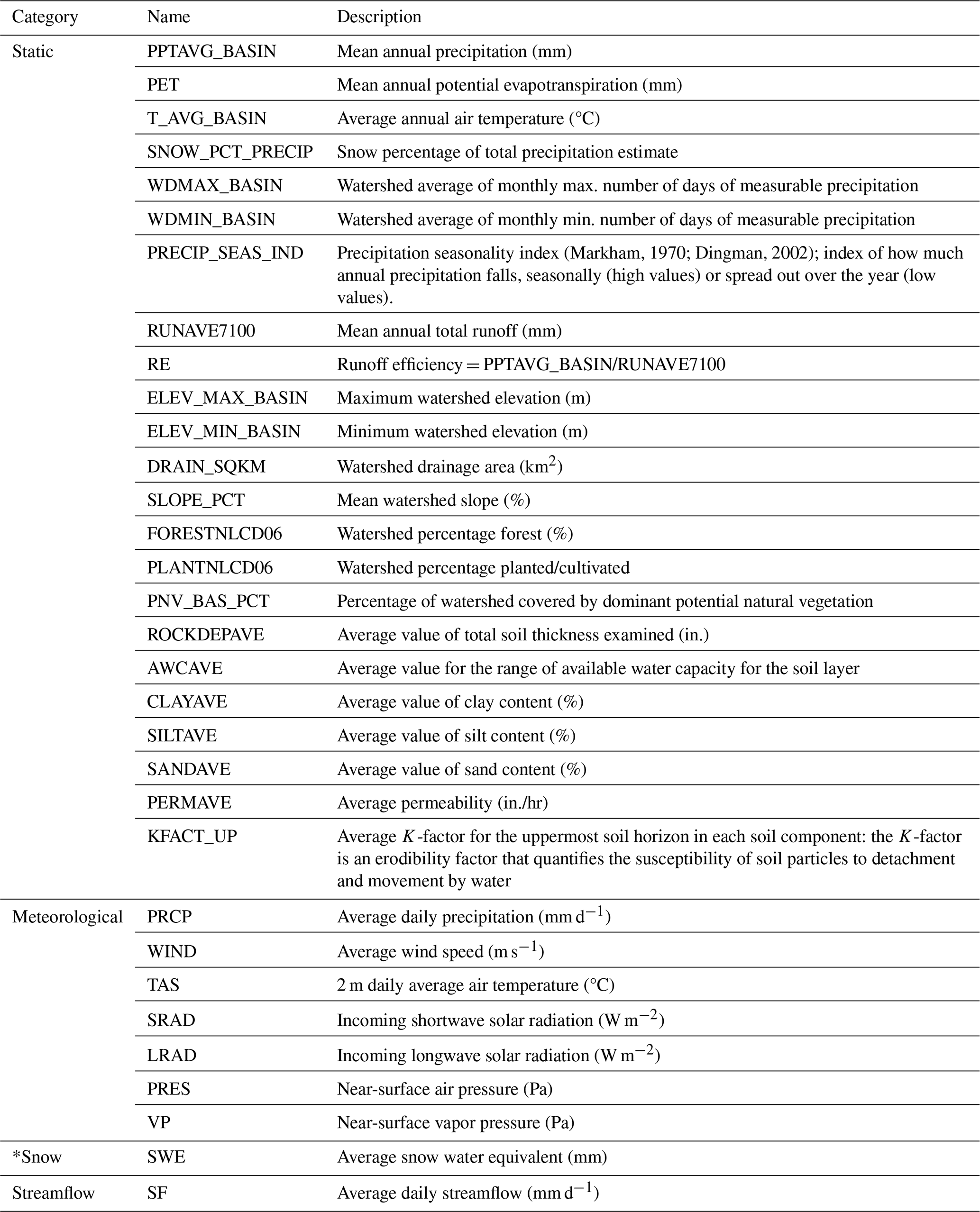
Table A3 LSTM hyperparameters used in this study (adapted from Kratzert et al., 2019; Modi et al., 2024).

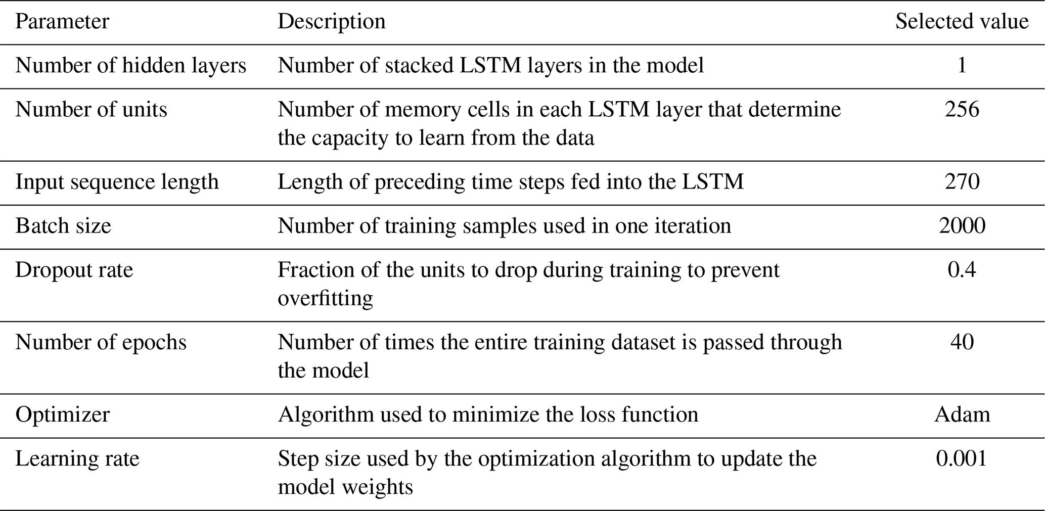
A3 Historical performance evaluation of our designed true forecast systems before and after calibration/training

As shown in Fig. A2, for WRFH, the improvements were minimal across most metrics before (WRFH_DEF) and after (WRFH_CAL) calibration, except for the variability (ratio of standard deviation), which improved from 1.65 to 1.25. With LSTM, major improvements were seen with the median daily NSE, improving from 0.58 to 0.77. In general, the improvements across all metrics for both models underscore the importance of model calibration and training, as seen with LSTM_FINAL and WRFH_CAL (Fig. A2).

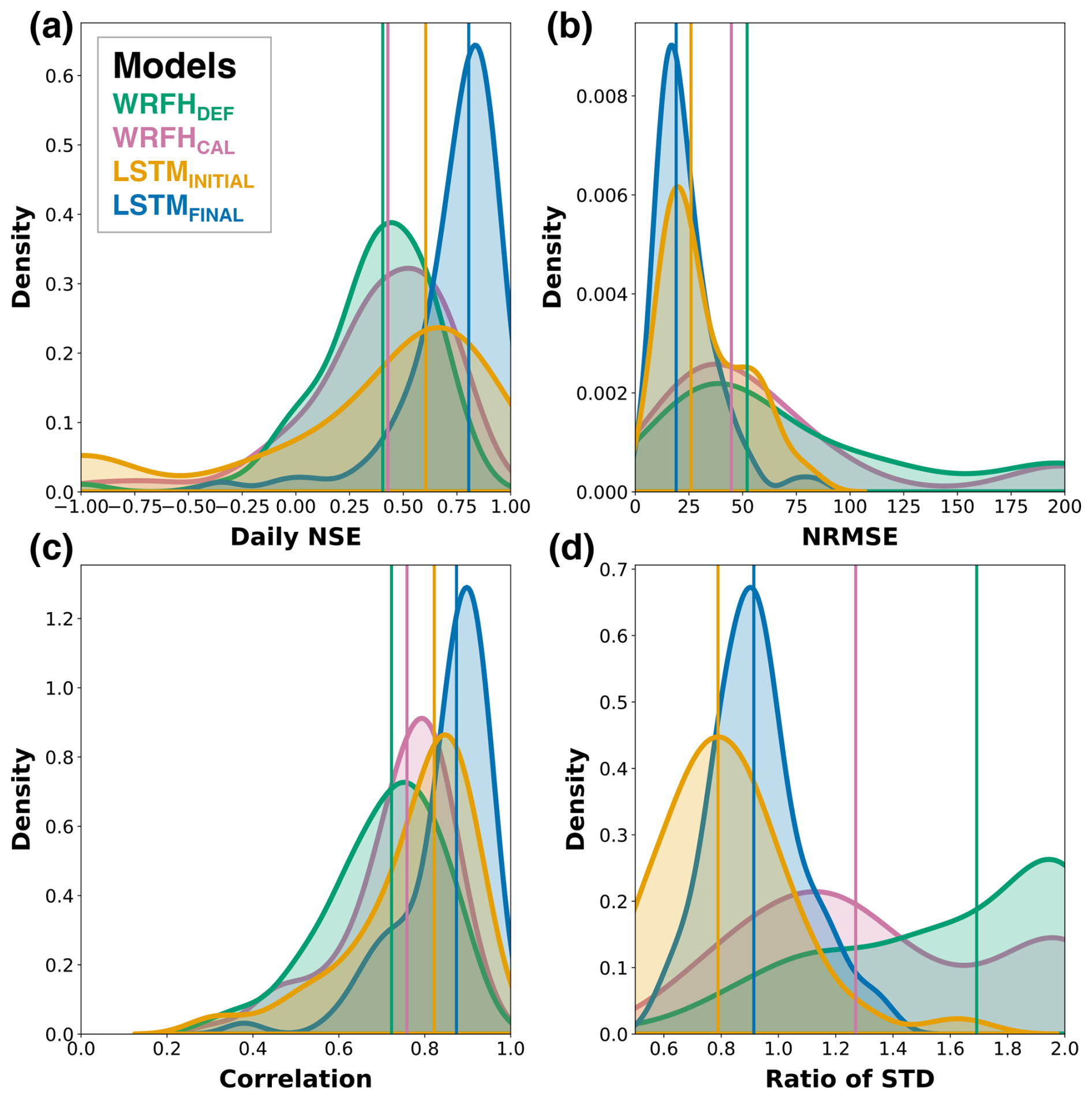
Figure A2 Historical model performance of true forecast systems for WRFH (default and calibrated) and LSTM (initial and final) models: (a) daily NSE, (b) NRMSE of the total April–July streamflow volumes, (c) daily correlation, (d) ratio of the standard deviation against observations. Comparison shown for the 76 basins during the testing period, WY2001–WY2010.

A4 Exposition of irregular error structures in true forecasts

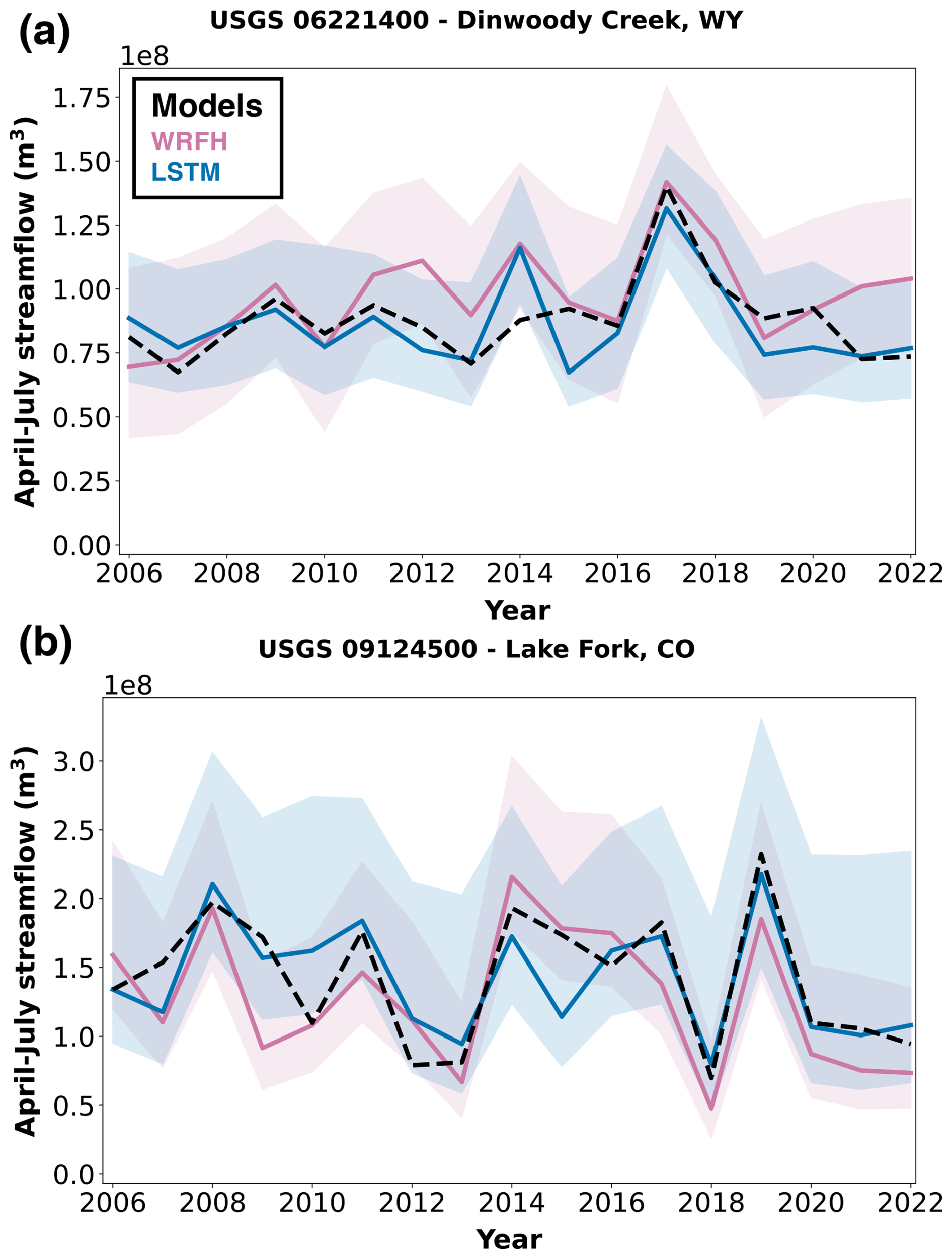
Figure A3 April–July streamflow volume from two true forecast systems (WRFH and LSTM) in WY2006–WY2022 at Dinwoody Creek (USGS 06221400) and Lake Fork (USGS 09124500).