Improving heat transfer predictions in heterogeneous riparian zones using transfer learning techniques

Data-driven deep learning models usually perform well in terms of improving computational efficiency for predicting heat transfer processes in heterogeneous riparian zones. However, traditional deep learning models often suffer from accuracy when data availability is limited. In this study, a novel physics-informed deep transfer learning (PDTL) approach is proposed to improve the accuracy of spatiotemporal temperature distribution predictions. The proposed PDTL model integrates the physical mechanisms described by an analytical model into the standard deep neural network (DNN) model using a transfer learning technique. To test the robustness of the proposed PDTL model, we analyze the influence of the number of observation points at different locations, streambed heterogeneity, and observation noise levels on the mean squared error MSE values between the observed and predicted temperature fields. Results indicate that the PDTL model significantly outperforms the DNN model in scenarios with scarce training data, and the MSE values decrease with increasing observation points for both PDTL and DNN models. Furthermore, increasing streambed heterogeneity and observation noise levels raises the MSE values of the PDTL and DNN models, with the PDTL model exhibiting greater robustness than the DNN model, highlighting its potential for practical applications in riparian zone management.

1 Introduction

Understanding heat transfer processes in riparian zones is critical for evaluating physical and biochemical processes during surface water–groundwater interactions, such as contaminant transport (Elliott and Brooks, 1997; Schmidt et al., 2011), water resource management (Bukaveckas, 2007; Fleckenstein et al., 2010), and aquatic ecosystem regulation (Ren et al., 2018; Halloran et al., 2016). As a primary source of uncertainty in riparian zone modeling, the inherent heterogeneity of the streambed stands out as a pivotal factor in accurately modeling groundwater flow and heat transfer processes (Karan et al., 2014; Brunner et al., 2017). However, given the intricacies of streambed heterogeneity, data acquisition in heterogeneous riparian zones is often time-consuming and costly (Zhang et al., 2023; Kalbus et al., 2006). Consequently, achieving accurate predictions of heat transfer processes in heterogeneous riparian zones with limited observation data remains challenging.

Over the past few decades, there has been a substantial increase in efforts toward simulating heat transfer processes in riparian zones, which can be categorized into two groups: physics-based models and data-driven models (Barclay et al., 2023; Feigl et al., 2021; Heavilin and Neilson, 2012). Typically, the physics-based models employ partial differential equations to characterize heat transfer dynamics within riparian zones, such as the convection–diffusion equation (Chen et al., 2018; Keery et al., 2007), which aims to simulate and forecast temperature variations within riparian zones. Resolving the convection–diffusion equation generally involves two approaches: analytical and numerical models. Analytical models provide a precise mathematical representation of heat transfer dynamics and offer fundamental insights into physical processes within riparian zones, but their applicability is often limited to rather simplified and idealized scenarios (Keery et al., 2007; Bandai and Ghezzehei, 2021; Zhou and Zhang, 2022). Numerical models, which rely on discretizing governing equations and solving them iteratively, are able to handle more intricate scenarios and address unsteady flows effectively (Cui and Zhu, 2018; Ren et al., 2019, 2023). Nevertheless, numerical models are constrained by the uncertainties of model structures and the prerequisites of streambed characteristic parameters (Heavilin and Neilson, 2012; Shi et al., 2023).

Data-driven models, unlike physics-based models, can create a direct mapping between input and output variables without explicit knowledge of underlying physical processes governing the system (Zhou and Zhang, 2023; Callaham et al., 2021). In recent years, data-driven models have achieved significant advancements and emerged as a successful alternative in hydrological and environmental modeling (Zhou et al., 2024; Cao et al., 2022; Wade et al., 2023). However, their deficiency in incorporating physical principles restricts their capability to delineate explicit computational processes as physics-based models, posing a challenge to achieve enhanced extrapolation capabilities (Read et al., 2019; Cho and Kim, 2022). Meanwhile, data-driven models typically require massive amounts of data for training and may yield results that defy established physical laws due to the lack of physical principles (Read et al., 2019; Xie et al., 2022). The strengths and weaknesses inherent in both data-driven and physically based models are evident across various research domains (Kim et al., 2021; Wang et al., 2023). Consequently, there is an increasing inclination towards integrating physical processes into data-driven models, which enables these models to extract patterns and laws from both observation data and underlying physical principles (Zhao et al., 2021; Karpatne et al., 2017).

Typically, several methods exist to integrate two divergent models: one is to employ a deep learning framework to substitute either a submodule or an intermediary parameter in physically based models (Jiang et al., 2020; Zhao et al., 2019; Cho and Kim, 2022; Arcomano et al., 2022), and the other involves integrating physical models to furnish additional constraints or penalizations to the deep learning framework (Kamrava et al., 2021; Raissi et al., 2019; Yeung et al., 2022). Additionally, transfer learning provides a feasible approach for integrating analytical and deep learning models, where knowledge is transferred from a distinct but relevant source domain to enhance the efficacy of the target domain (Zhang et al., 2023; Chen et al., 2021). This approach can diminish the requirement for extensive training data in the target domain, which is considered to be a major barrier of deep learning applications. By leveraging knowledge gained from pre-training models, it accelerates the learning process and enhances model performance (Guo et al., 2023; Jiang and Durlofsky, 2023). Recently, the use of the transfer learning technique has gained attention in the field of hydrological modeling (Zhang et al., 2023; Cao et al., 2022; Chen et al., 2021; Vandaele et al., 2021; Willard et al., 2021). For example, Xiong et al. (2022) developed a long short-term memory (LSTM) model of daily dissolved inorganic nitrogen concentrations and fluxes in the coastal watershed located in southeastern China. They retrained this model using multi-watershed data and successfully applied it to seven diverse watersheds through a transfer learning approach. Zhang et al. (2023) used the transfer learning technique to integrate the deep learning model and analytical models for predicting groundwater flow in aquifers and obtained satisfactory prediction performance for complex scenarios.

In this study, we introduce a novel physics-informed deep transfer learning (PDTL) approach that incorporates physical information from analytical models into a deep learning framework using the transfer learning technique. The proposed PDTL model is implemented to predict the spatiotemporal temperature distribution in heterogeneous riparian zones by leveraging analytical solutions, deep learning models, and transfer learning techniques. The analytical model is used to efficiently produce physically consistent heat distribution patterns and data in homogeneous riparian zones, which serve as the training data for the pre-training deep learning model. Subsequently, the weights and biases learned from the pre-training model are transferred to a new deep learning model under heterogeneous scenarios through transfer learning. By integrating insights from analytical models with the approximation capability of deep learning models, the PDTL model achieves improved efficiency and performance. Notably, the newly proposed approach demonstrates significant performance improvement, even with scarce observational data. This innovative approach provides for accurate and efficient modeling of complex heat transfer processes in heterogeneous environments, even with limited observation data.

2 Methods

2.1 Conceptual model

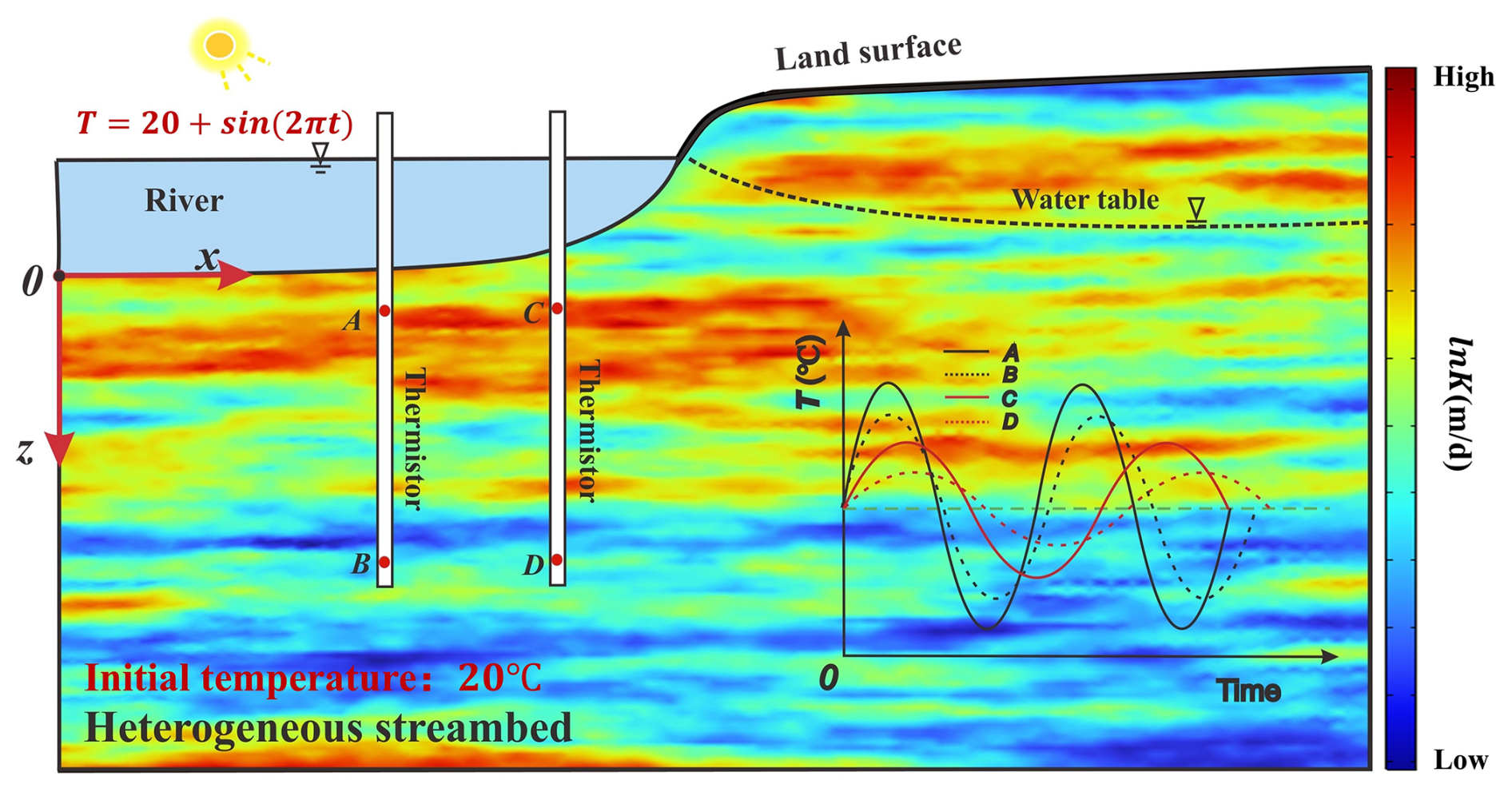
The two-dimensional (2D) conceptual model of the heat transfer process in a heterogeneous streambed is depicted in Fig. 1. The coordinate system originates at the center of the river, with the x axis oriented horizontally from left to right along the streambed. The z axis is located vertically downward along the left inlet boundary of the system and perpendicular to the x axis. It is postulated that the thermal properties of the streambed are uniform. The river has a width of 2L. Heat originated from the river, with its temperature represented by an arbitrary function. The initial and boundary conditions are depicted in Fig. 1. An initial temperature of 20 °C is prescribed. The boundary conditions on the left, right, and bottom sides are all specified as no heat flux boundary. The top boundary condition at $\mathrm{0}\le x\le L$ (L=0.32 m in this study) is represented by a sinusoidal temperature signal ranging between 19 and 21 °C (i.e., $f\left(t\right)=\mathrm{20}+\sin \left(\mathrm{2}\mathit{\pi }t\right)\mathrm{°}\mathrm{C}$). Meanwhile, the top boundary condition at x>L is held constant at a temperature of 20 °C. For this conceptual framework, two modeling approaches are employed. The analytical model provides exact solutions for heat transfer in homogeneous streambeds with uniform hydraulic conductivity and thermal properties (Shi et al., 2023). It generates physically consistent temperature distributions efficiently for the pre-training phase of our PDTL model. Meanwhile, the numerical model extends this solution to heterogeneous streambeds with spatially variable hydraulic conductivity, accommodating complex flow paths created by streambed heterogeneity. The details of the analytical solution for the homogeneous streambed and the numerical solution for the heterogeneous streambed are available in the Supplement.

Figure 1 Schematic diagram of the temperature distribution in the riparian zones.

2.2 Deep neural network (DNN)

The deep neural network (DNN) is a multi-layer feed-forward network with an input layer, multiple hidden layers, and an output layer. The backpropagation algorithm is utilized to minimize the mean error of the output and has been proven to be crucial in enhancing convergence (Jin et al., 2024). Assuming the presence of m hidden layers, the input and output vectors are denoted by X and O, respectively. The forward equations of the DNN model can be represented as follows:

$$\begin{array}{}\text{(1a)}& {\displaystyle }& {\displaystyle }{H}_i=\tanh (W_{i}X+b_i)i=\mathrm{1},\mathrm{\dots },m,\text{(1b)}& {\displaystyle }& {\displaystyle }O=\tanh (W_{m+\mathrm{1}}X+b_{m+\mathrm{1}}),\end{array}$$

where H_i represents the output of the ith hidden layer and W and b represent the weight matrices and bias vectors, respectively. Typically, W and b can amalgamate as the parameter set $\mathit{\theta }=\mathit{\{}{W}_i,b_i{\mathit{\}}}_{i=\mathrm{1}}^{m+\mathrm{1}}$, and tanh refers to the tanh activation function. To mitigate the impact of dimensionality during the training process, the temperature field dataset is normalized to $[-\mathrm{1},\mathrm{1}]$ through the following equation in the pre-training process:

$$\begin{array}{}\text{(2)}& D_{\text{norm}}=\mathrm{2}{\displaystyle \frac{D-D_{\text{min}}}{D_{\text{max}}-D_{\text{min}}}}-\mathrm{1},\end{array}$$

where D denotes data utilized in the DNN model and D_max and D_min denote the maximum and minimum values and are computed with reference to the training samples exclusively. The same values of D_max and D_min are employed to normalize the testing samples to prevent data leakage (Zuo et al., 2020).

2.3 Deep collocation method

The collocation technique uses a collection of randomly distributed points to minimize the loss function while adhering to a specified set of constraints. This method demonstrates a degree of immunity against instabilities, such as explosion or vanishing gradients encountered in DNNs, offering a feasible strategy for training DNNs (Guo et al., 2023). By incorporating the collocation points throughout the model domain, along with the physical principles of the boundary and initial conditions, the learning process aims to minimize the following loss functions:

$$\begin{array}{}\text{(3a)}& {\displaystyle }& {\displaystyle }L\left(\mathit{\theta }\right)={\text{MSE}}_{\mathrm{D}}+{\text{MSE}}_{\text{BC}}+{\text{MSE}}_{\text{IC}},\text{(3b)}& {\displaystyle }& {\displaystyle }{\text{MSE}}_{\mathrm{D}}={\displaystyle \frac{{\mathit{\xi }}_{\mathrm{D}}}{N_{\mathrm{D}}}}\sum _{i=\mathrm{1}}^{N_{\text{IC}}}\Vert T_{\mathrm{N}}(x_i,y_i,t_i;\mathit{\theta })-T(x_i,y_i,t_i){\Vert }^{\mathrm{2}},\text{(3c)}& {\displaystyle }& {\displaystyle }{\text{MSE}}_{\text{BC}}={\displaystyle \frac{{\mathit{\xi }}_{\text{BC}}}{N_{\text{BC}}}}\sum _{i=\mathrm{1}}^{N_{\text{BC}}}\Vert T_{\mathrm{N}}(x_i,y_i,t_i;\mathit{\theta })-G(x_i,y_i,t_i){\Vert }^{\mathrm{2}},\text{(3d)}& {\displaystyle }& {\displaystyle }{\text{MSE}}_{\text{IC}}={\displaystyle \frac{{\mathit{\xi }}_{\text{IC}}}{N_{\text{IC}}}}\sum _{i=\mathrm{1}}^{N_{\text{IC}}}\Vert T_{\mathrm{N}}(x_i,y_i,\mathrm{0};\mathit{\theta })-T(x_i,y_i,\mathrm{0}){\Vert }^{\mathrm{2}},\end{array}$$

where L(θ) refers to the total loss; MSE_D, MSE_BC, and MSE_IC represent the mean squared error (MSE) of the model domain, boundary conditions, and initial conditions, respectively; N_D, N_BC, and N_IC are the number of data points for different terms; and ξ_D, ξ_BC, and ξ_IC are scaling factors to normalize loss terms. According to the study of He and Tartakovsky (2021), the values of ξ_D, ξ_BC, and ξ_IC in this study are set to 1, 10, and 10, respectively. $T_{\mathrm{N}}(x_i,y_i,t_i)$ represents the values estimated by the DNN model; $T(x,y,t)$ is the solution of the 2D analytical model with boundary conditions $G(x,y,t)$ and initial conditions T(xy,0). The objective is to find the parameter set θ that minimizes the loss function. L(θ) considers the constraints of physical principles and imposes penalties for initial and boundary conditions. It allows the neural networks to learn the underlying physical principles and the boundary and initial conditions rather than simply memorizing the training data, thus improving the efficiency and accuracy (He and Tartakovsky, 2021; Raissi et al., 2020; Tartakovsky et al., 2020).

2.4 Transfer learning

As depicted in Fig. 2, traditional deep learning models are allocated to distinct learning tasks, which require each model to be trained independently from scratch, leading to high computational demands and the need for substantial amounts of training data for each task. In contrast, the transfer learning technique offers an efficient alternative. By employing a pre-trained model that is then fine-tuned for predicting heat transfer in heterogeneous streambeds, transfer learning can significantly reduce the computational burden and the need for large datasets. This is achieved by leveraging the knowledge gained from the source domain and applying it to the target domain, thereby accelerating the learning process and improving the model performance.

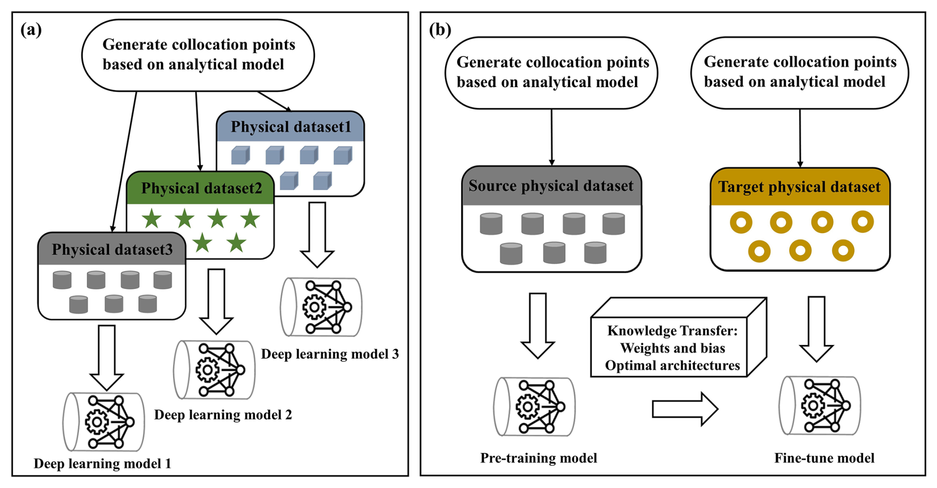
Figure 2 Schematic diagram of the pre-training and fine-tuning methods in the transfer learning model (revised from Guo et al., 2023). (a) Traditional machine learning method. (b) Transfer learning method.

The transfer learning technique involves training a model to establish a mapping between the input vector X and the observed data O derived from a target dataset $D=\mathit{\left\{}\right(X_i,O_i{)}_{i=\mathrm{1}}^n$, $X_i\in X,O_i\in O\mathit{\}}$. It assumes that both the source and target tasks share similar parameters or prior distributions of the hyperparameters. The pre-training model is established utilizing the dataset from the source tasks $D_{\mathrm{s}}=\mathit{\left\{}\right(X_{\mathrm{s}},O_{\mathrm{s}}{)}_{s=\mathrm{1}}^n$, X_s∈X, O_s∈O}, which is generated through analytical or numerical models. In this study, the source and target datasets are spatiotemporal distributions of temperature fields in homogeneous and heterogeneous streambeds, respectively. The analytical model developed by Shi et al. (2023) is employed to provide a training dataset for pre-training. However, for the heterogeneous streambed, the analytical model is not available; the numerical models are employed to generate the fine-tuning dataset and serve as the benchmarks to evaluate the performance of the proposed PDTL model. The parameter θ_T for the fine-tuning model is acquired through the optimization of the loss function delineated by

$$\begin{array}{}\text{(4)}& {\mathit{\theta }}_{\text{T}}=\underset{{\mathit{\theta }}_{\mathrm{T}}}{\text{argmin}}\sum _{i=\mathrm{1}}^{n^{\ast }}{\displaystyle \frac{\mathrm{1}}{n^{\ast }}}\left|f_t\right(X_t;{\mathit{\theta }}_{\text{T}})-O_t{|}^{\mathrm{2}},\end{array}$$

where n^∗ denotes the number of training datasets employed to fine-tune the pre-training model and f_t() denotes the predictive function of the fine-tuning model.

The flowchart of the newly proposed framework is summarized in Fig. 3: the PDTL model is developed by initially generating an input dataset using the analytical model for heat transfer in homogeneous streambeds. The dataset is subsequently employed to pre-train a DNN model with physical constraints, focusing on learning the weights and biases of the fully connected layer. Next, the data of the observation points in the corresponding numerical model for heat transfer in heterogeneous streambeds are utilized to fine-tune the pre-trained DNN model by transferring the learned insensitive layers (i.e., freezing their weights and biases) and retraining the learnable parameters of the remaining layers. Finally, the effectiveness of the PDTL model is evaluated by comparing its performance against a traditional DNN model with a different number of observation points, which evaluates the model's ability to predict the spatiotemporal temperature distribution in heterogeneous streambeds.

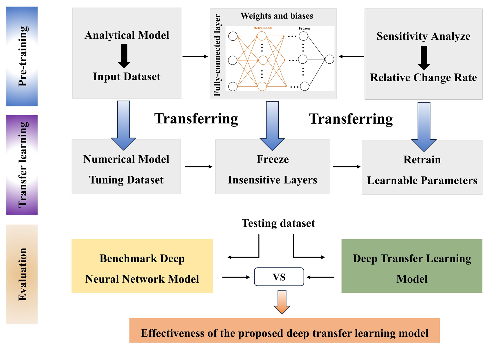
Figure 3 Proposed PDTL framework used in this study. The framework consists of a pre-training module, a transfer learning module, and an evaluation module.

3 Results

3.1 Pre-training process

In this study, the pre-training model is a DNN model with six hidden layers, each containing 16 neurons. To evaluate the sensitivity of weights and biases to hydraulic conductivity and to identify which layers should be trainable or remain frozen, two pre-training models with identical structures but varying hydraulic conductivities are constructed. Both datasets consist of a 100×100 grid with 100 time steps generated by the 2D analytical model, where 80 % of the dataset is utilized for training and the remaining 20 % is utilized for testing. q_x and q_z depend on hydraulic conductivities in x and z directions. In this section, q_x and q_z are set to $\mathrm{0.2}m/d$, $\mathrm{0.3}m/d$ and $\mathrm{0.6}m/d$, $\mathrm{0.9}m/d$ for these two models, respectively. The input data consist of spatial locations (x,y) and time t, while the output data consist of the corresponding temperature. Results indicate that the predictions of the two pre-training models closely align with the analytical model with average MSE values of $\mathrm{1.2}\times {\mathrm{10}}^{-\mathrm{6}}$ and $\mathrm{1.5}\times {\mathrm{10}}^{-\mathrm{6}}$, respectively. Similarly to the works of Hu et al. (2020) and Zhang et al. (2023), the difference in weights and biases between the two pre-training models is evaluated using the relative change rate (RCR):

$$\begin{array}{}\text{(5)}& \text{RCR}={\displaystyle \frac{\mathrm{1}}{I}}\sum _i^I{\displaystyle \frac{|{\mathit{\theta }}_{\mathrm{1}i}-{\mathit{\theta }}_{\mathrm{2}i}|}{{\mathit{\theta }}_{\mathrm{1}i}}},\end{array}$$

where θ_1i and θ_2i are parameter matrixes in two pre-training models, respectively, and I is the number of elements in the parameter matrix. For enhanced comparability and credibility, each of the two pre-training models undergoes 20 training processes. Figure 4 presents the average RCR of weights and biases across all layers for the two pre-training models over 20 trials. The RCR of biases shows consistent stability across all layers, except for layer 3. In contrast, variations in weights are more prominent, particularly in layers 1, 2, and 3, which underscores the heightened sensitivity of these layers to hydraulic conductivity. Consequently, layers 1, 2, and 3 of the pre-training models are marked as trainable, while the remaining layers are held frozen in the following analysis. Notably, the convergence criteria are defined as a threshold of 3000 iterations with a minimum gradient alteration of $\mathrm{5}\times {\mathrm{10}}^{-\mathrm{6}}$ throughout the training phase (Zhang et al., 2023; Wang et al., 2021).

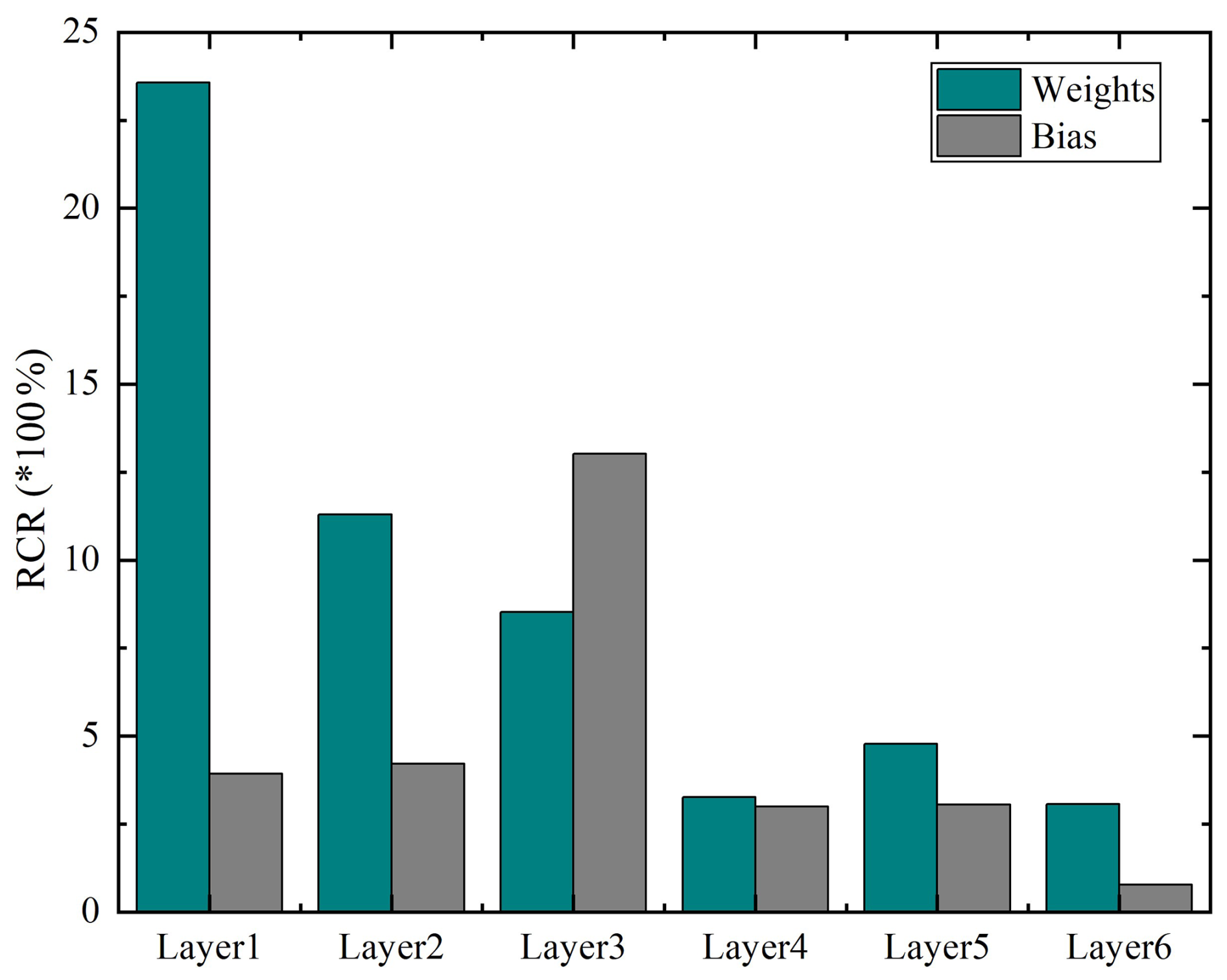
Figure 4 The average relative change rate (RCR) of weight when pre-training the neural network with different K values.

3.2 Spatial and temporal performance for the homogeneous scenario

The spatiotemporal distribution of temperature in homogeneous streambeds is obtained by the analytical model. In this study, we use 1, 5, 10, 20, 50, and 100 observation points, each with 100 time steps. The hydrological parameters are set at $q_x=\mathrm{0.4}m/d$ and $q_z=\mathrm{0.6}m/d$, with all other parameters being consistent with those presented in Fig. 1. The temperature data from these observation points are used as training data for PDTL and DNN. The reference temperature field on 0.5d (i.e., the 50th time step) is employed as testing data. Figure 5 illustrates the absolute errors of the PDTL and DNN models for the homogeneous riparian zone. The results suggest that the PDTL model aligns well with the reference temperature field, whereas the DNN model tends to struggle in accurately capturing the reference temperature field. This highlights the significant improvement in the performance of the deep learning model facilitated by prior knowledge of the analytical solution and physical information. The pre-training model incorporates physical knowledge to provide superior initial parameters (weights and biases), which narrows the search space during the fine-tuning process. In contrast, the DNN model randomly initializes these parameters and requires more training points to explore the entire parameter space. To further demonstrate the predictive performance of the proposed model in time series, Fig. 6 shows the temperature time series predicted by the PDTL and DNN models at a given observation point (x=0.5m, y=0.5m). Results indicate that the PDTL model predicts the temperature fluctuation trend better compared to the DNN model. Especially for the sparse dataset with a few observation points, the average MSE of the PDTL model with 5 observation points is approximately 3.2 times lower than that of the DNN model. As shown in Fig. S2 in the Supplement, there is no significant difference in the performance of the PDTL and DNN models when the number of observation points increases to 200. Notably, the performance of the PDTL model appears to be less sensitive to the number of observation points. We attribute this phenomenon to two factors: (1) randomly selected observation points lead to optimal performance when the observation points are in proximity to the test point and vice versa; (2) the PDTL model demonstrates the capacity to integrate substantial information from the analytical model, which diminishes the requirement for the number of observation points.

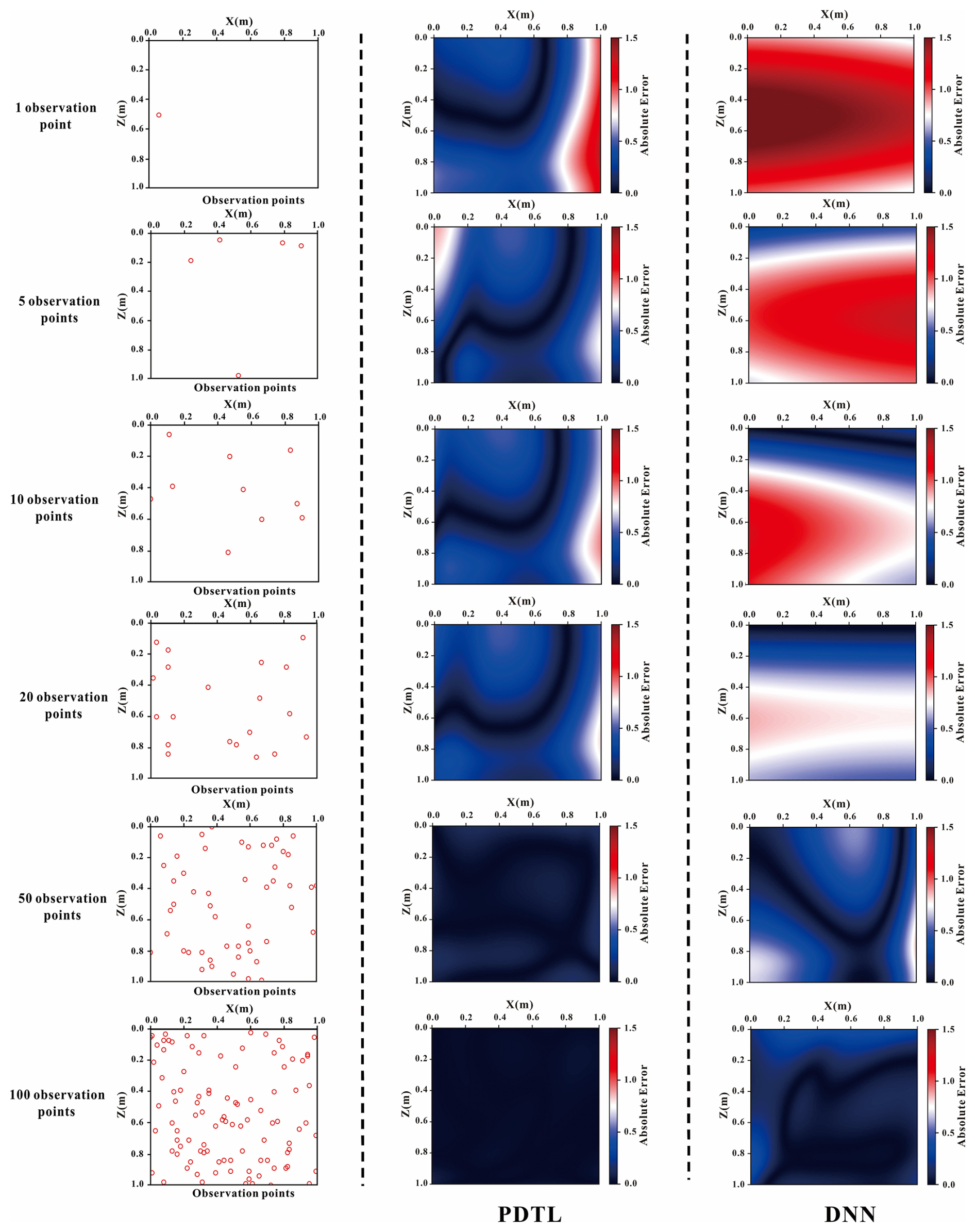
Figure 5 Absolute errors between the predicted temperature field and reference temperature field using PDTL and DNN models for the homogeneous streambed.

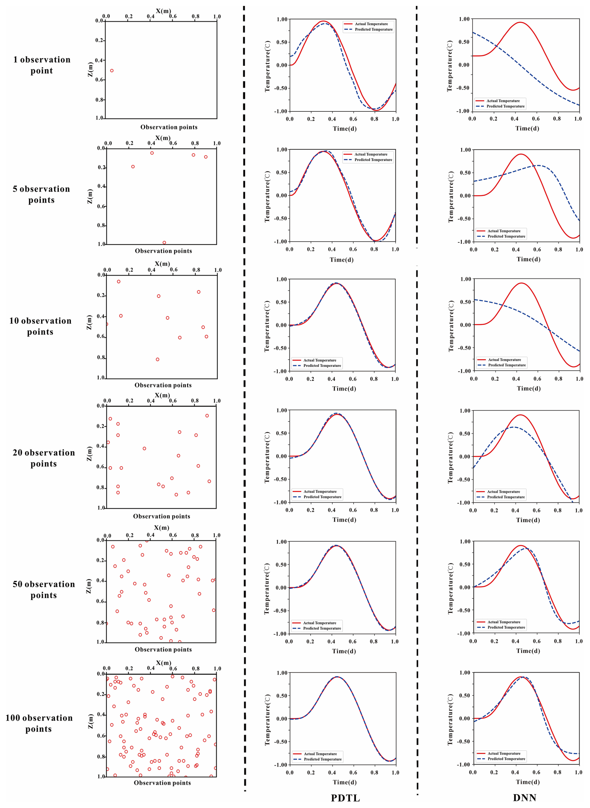
Figure 6 Comparisons of the predicted temperature (blue curves) and reference temperature (red curves) using PDTL and DNN models for the homogeneous streambed.

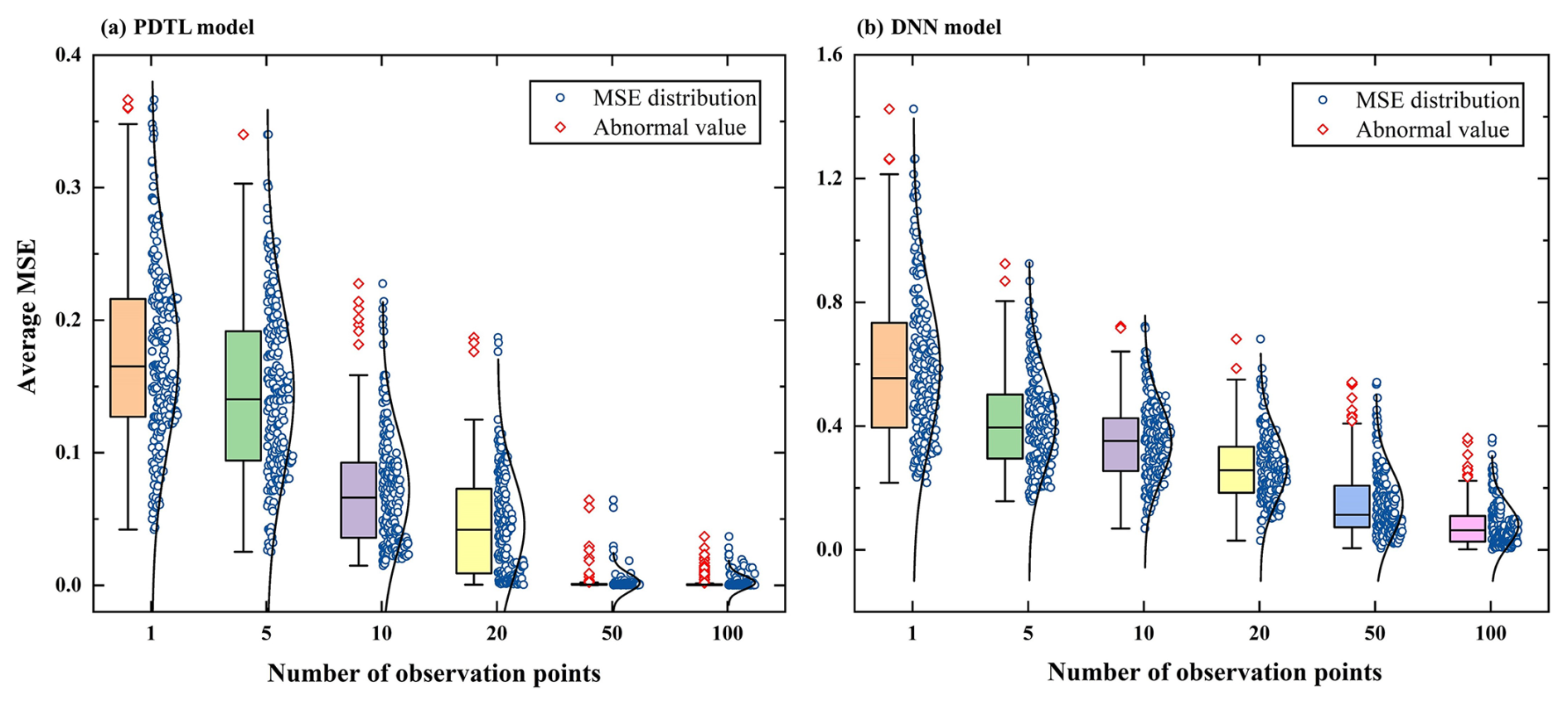
Figure 7 MSE distribution of normalized results from PDTL and DNN models plotted against the number of observation points for the homogeneous streambed. (a) PDTL model. (b) DNN model.

The choice of observation points can influence the outcomes of the proposed PDTL model. To mitigate the effect of their positions, each observation point is randomly generated 200 times. The distributions of the average MSE for both the PDTL and DNN models across diverse numbers of observation points are illustrated in Fig. 7. Results reveal that both the interquartile range and the mean values of MSE for the PDTL model are considerably smaller than those of the DNN model. As an illustration, when considering 10 observation points, the average MSE for the PDTL model is approximately 0.11, whereas that for the DNN model is 0.54. Furthermore, there is a significant reduction in both interquartile range and mean values of MSE of the PDTL model, and the interquartile range and mean values of MSE of the PDTL model tend to stabilize as the number of observation points exceeds 50. On the contrary, the interquartile range and mean values of MSE of the DNN model consistently decrease with an increasing number of observation points, displaying a consistent pattern as observed in Fig. 6. It should be emphasized that the PDTL model can still produce satisfactory results even with sparse data. Even with more than 50 observation points, the DNN model still underperforms the PDTL model, which can be attributed to the following reasons: (1) due to the lack of prior physical knowledge, the DNN model may require more data to learn relatively complex patterns; (2) both the PDTL and DNN models follow the identical convergence criterion with a restricted number of epochs during the fine-tuning process, which may result in incomplete training for the DNN model.

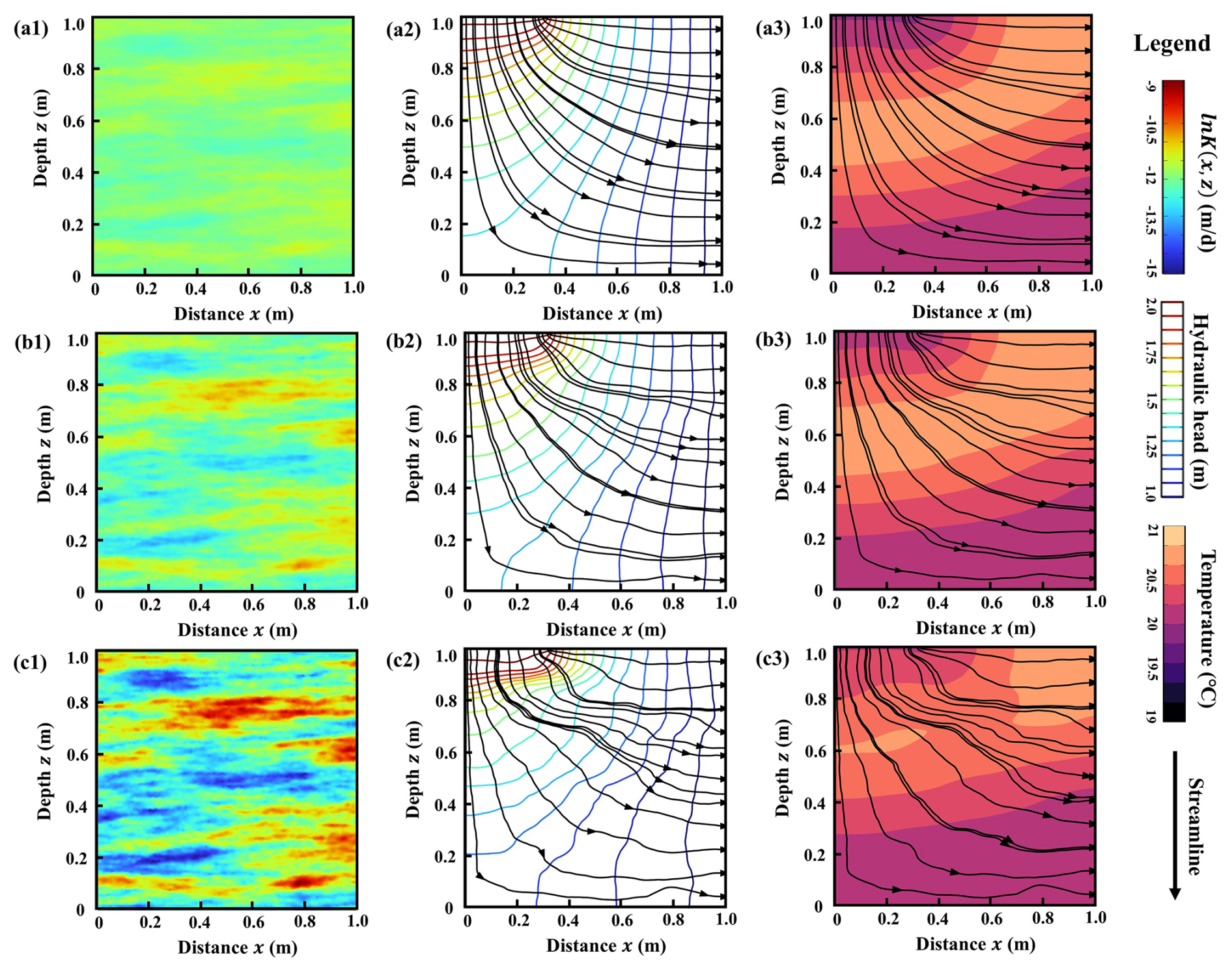
Figure 8 Heat map and the contours of hydraulic head, temperature field, and streamlines for different K fields. Panels (a1)–(c1) show the heat map of K fields, panels (a2)–(c2) show the contours of hydraulic head and streamlines at 0.5d, and panels (a3)–(c3) show the contours of temperature field and streamlines at 0.5d for ${\mathit{\sigma }}_{\text{lnk}}^{\mathrm{2}}=\mathrm{0.2}$, 0.5, and 1.0, respectively.

3.3 Effects of nonuniform flow on heat transfer

In this section, we evaluate the performance of the PDTL model in predicting the spatiotemporal temperature distribution in heterogeneous streambeds. The heterogeneous lnK field is generated by the exponential covariance function with mean μ=0; correlation length l=0.1 m in both the x and z directions; and variance ${\mathit{\sigma }}_{\text{lnK}}^{\mathrm{2}}=\mathrm{0.2}$, 0.5, and 1.0, respectively. Accordingly, three scenarios with low to high heterogeneity are created. Figure 8 depicts the random lnK fields and references flow fields of the three scenarios. The other parameters remain consistent with those of the homogeneous streambed. The temperature distribution in the heterogeneous streambed is estimated using the numerical model. Temperature time series of 1, 5, 10, 20, 50, and 100 observation points are extracted to fine-tune both the PDTL and DNN models.

To mitigate the impacts of random sampling during the fine-tuning process, 200 stochastic simulations are performed. The distribution of the average MSE for both the PDTL and DNN models in three distinct heterogeneous streambeds from low to high heterogeneity are shown in Fig. 9. One can find that the average MSE of the PDTL model is consistently minimal and significantly lower than that of the DNN model. Besides, with the same number of observation points, a decrease in ${\mathit{\sigma }}_{\text{lnK}}^{\mathrm{2}}$ corresponds to a reduction in average MSE. These findings can be explained by the fact that the proposed PDTL model exhibits a strong ability to transfer knowledge between two datasets with similar structures or features. A decreased ${\mathit{\sigma }}_{\text{lnK}}^{\mathrm{2}}$ indicates less heterogeneity in the lnK field, resulting in a temperature field that more closely resembles those generated by the analytical model. We attribute this improvement in the PDTL model to the enhanced initial parameters of the DNN model through the incorporation of physical knowledge during the fine-tuning process. For both the PDTL and DNN models, the interquartile ranges and mean values of MSE decrease as the number of observation points increases. Notably, by leveraging the insights from the analytical model, the PDTL model can effectively predict the temperature distribution in heterogeneous streambeds, even with sparse observation points (e.g., 5 observation points). In contrast, while the DNN model exhibits improved performance with an increased number of observation points, its performance heavily relies on this factor, showing unsatisfactory outcomes with fewer observation points. When the number of observation points reaches 50, the interquartile range and MSE of the PDTL model exhibit marginal changes, but the interquartile range and MSE of the DNN model still decrease significantly. Furthermore, there is no significant difference in the performance of the PDTL and DNN models in heterogeneous scenarios when the number of observation points increases to 200, as shown in Figs. S3 and S4 in the Supplement. The average MSE of the PDTL model is approximately 2.8–18.4 times smaller than that of the DNN model with the same observation points, which further demonstrates the capability of the PDTL model to transfer knowledge from homogeneous environments to heterogeneous environments.

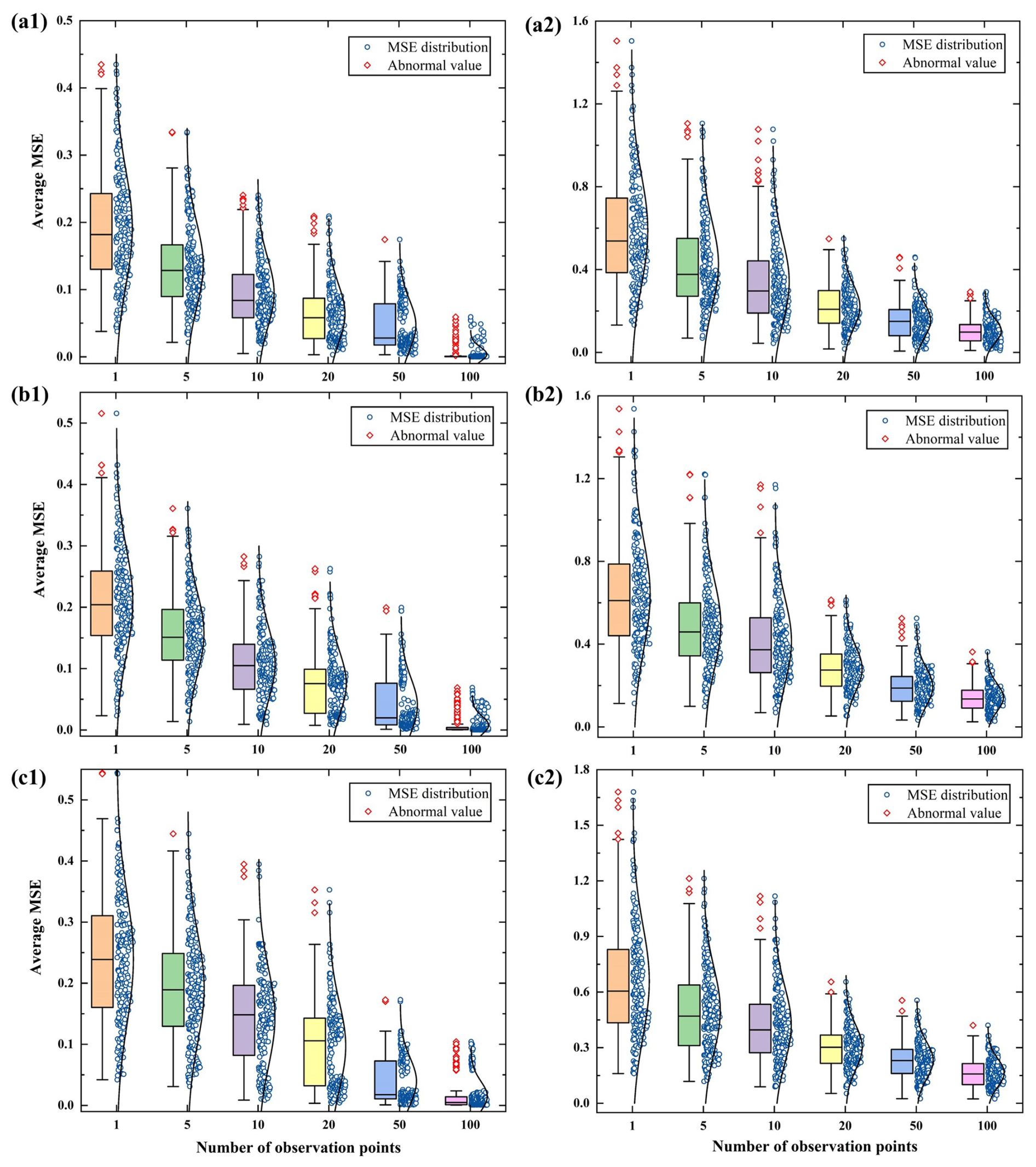
Figure 9 MSE distribution of normalized results from PDTL and DNN models plotted against the number of observation points for different heterogeneous streambeds. Panels (a1)–(c1) show the PDTL model and panels (a2)–(c2) show the DNN model for ${\mathit{\sigma }}_{\text{lnk}}^{\mathrm{2}}=\mathrm{0.2}$, 0.5, and 1.0, respectively.

3.4 Effects of river temperature uncertainty

In this section, we evaluate the effectiveness of the PDTL model in the context of river temperature observation noises, which may arise from suboptimal field conditions or sensor resolution limitations (Chen et al., 2022; Shi et al., 2023). Specifically, the white Gaussian noise is introduced at the top boundary:

$$\begin{array}{}\text{(6)}& f\left(t\right)=\mathrm{20}+\sin \left(\mathrm{2}\mathit{\pi }t\right)+\text{normrnd}({\mathit{\phi }}_{\text{Noise}},{\mathit{\sigma }}_{\text{Noise}}),\end{array}$$

where φ_Noise and σ_Noise denote the mean and variance of white Gaussian noise, respectively, and normrnd() denotes the Gaussian distribution. In this section, φ_Noise is set to 0 °C and σ_Noise is set to 0.025, 0.05, and 0.075 °C, as shown in Fig. 10. Similarly, the heterogeneous lnK field of streambed is generated by the exponential covariance function with μ=0, l=0.1 m in both x and z directions and ${\mathit{\sigma }}_{\text{lnK}}^{\mathrm{2}}=\mathrm{0.5}$. The temperature time series from diverse numbers of observation points (1, 5, 10, 20, 50, and 100) are utilized as training datasets for both PDTL and DNN models. Additionally, 200 stochastic simulations are conducted to mitigate the influence of random sampling of observation points during the fine-tuning process.

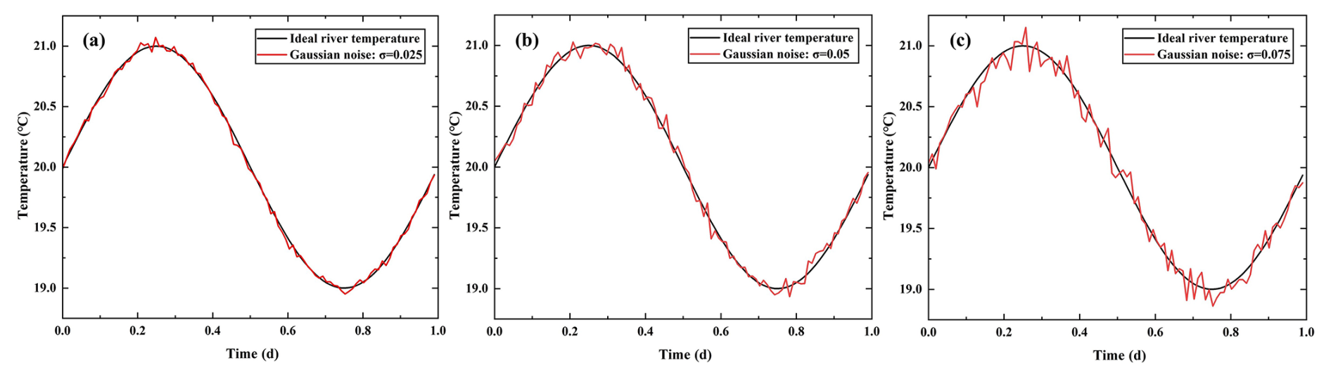
Figure 10 Time series diagram of river temperature under different observation noises. (a) σ=0.025 °C; (b) σ=0.05 °C; (c) σ=0.075 °C.

Figure 11 shows the distributions of the average MSE for both the PDTL and DNN models under different noise levels. It is observed that the PDTL and DNN models exhibit sensitivity to noise, and the elevated noise levels result in diminished model performance. Nevertheless, the PDTL model is less impacted by river temperature uncertainty compared to the DNN model. For instance, in cases of 10 observation points, the average MSE of the DNN model varies from 0.59–0.45 as σ decreases from 0.075–0.025. In contrast, the average MSE of the PDTL model ranges only from 0.11–0.08 under the same conditions, demonstrating the superior robustness of the PDTL model over the DNN model.

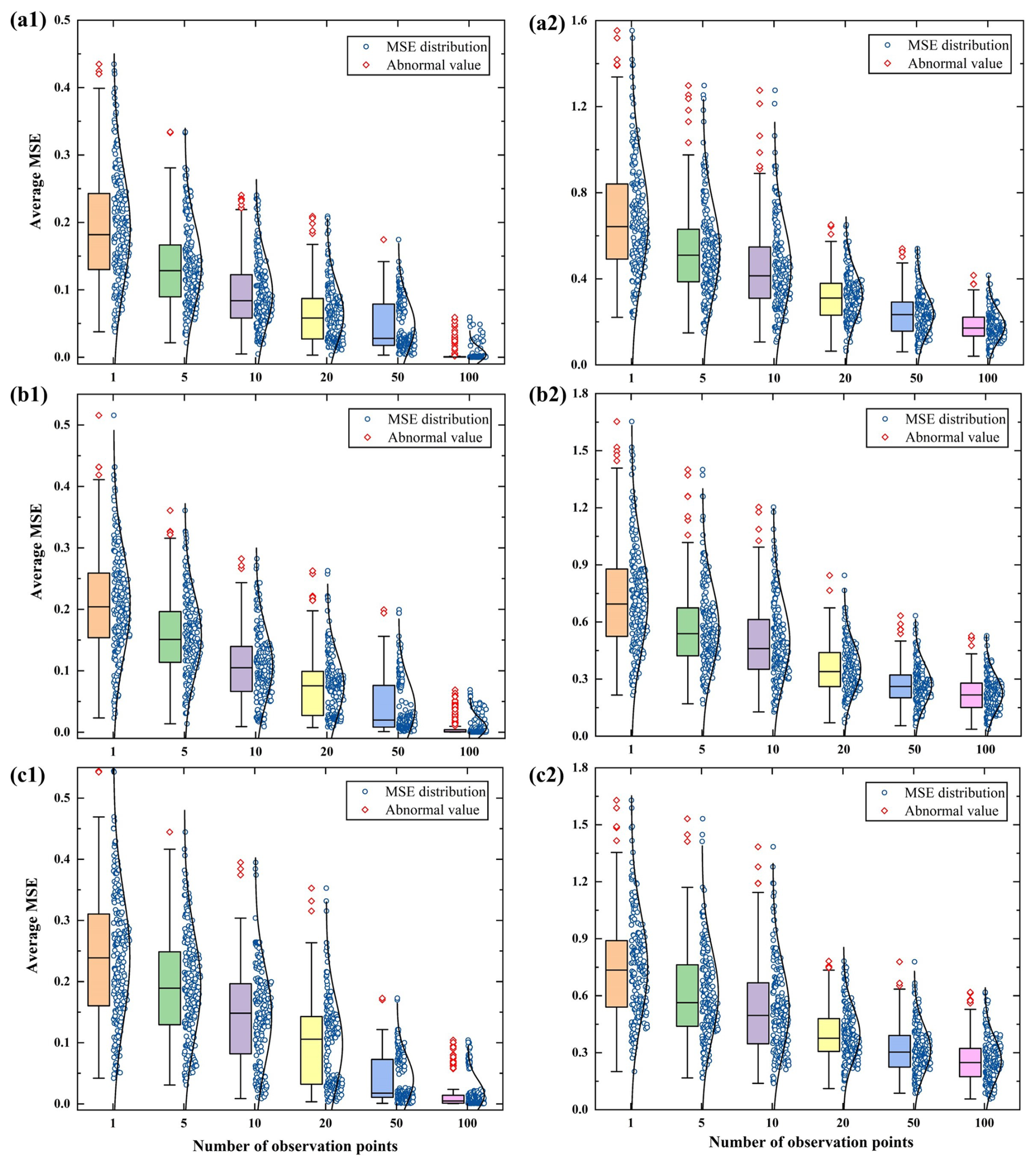
Figure 11 MSE distribution of normalized results from PDTL and DNN models plotted against the number of observation points for different observation noises. Panels (a1)–(c1) show the PDTL model and panels (a2)–(c2) show the DNN model for σ=0.025, 0.05, and 0.075 °C, respectively.

4 Discussion

This study investigates the effects of streambed heterogeneity, temperature observation noises, and the number of observation points at different locations on the performance of the proposed PDTL model. Results indicate that the proposed PDTL model exhibits robust prediction performance with significantly reduced interquartile range and MSE, particularly in scenarios with sparse data. These findings suggest that integrating analytical knowledge effectively decreases model uncertainties. Compared to conventional data-driven models, which often require extensive training data, the PDTL model leverages analytical knowledge to improve accuracy while reducing uncertainty. This highlights its potential advantages in environmental and hydrological studies where data collection is often constrained. A key strength of this framework is its transferability to other applications beyond heat transfer in riparian zones. By integrating analytical knowledge with a data-driven approach, it can be extended to solute transport processes and heat transfer in other heterogeneous porous media, such as groundwater contaminant migration and CO₂ geological storage. This versatility highlights the framework's potential for broader applications across various fields within environmental and hydrological studies. However, scientists should carefully consider the choice of training data and the assumptions underlying the analytical solutions when applying this framework to different settings.

Despite its advantages, it is imperative to recognize several constraints associated with the PDTL model proposed in this study. Firstly, the incapacity for extrapolation of the PDTL model restricts its applicability. As it lacks observation points outside the training domain, the PDTL model tends to face limitations concerning extrapolative tasks. Secondly, this study centers on modeling heat transfer problems in heterogeneous riparian zones, and the effectiveness of the PDTL model may be influenced by the selection of the K value. Thirdly, using locations as inputs may limit the model's transferability to other sites and weaken its direct connection to measurable physical variables. Future work will incorporate additional physically measurable parameters, such as surface temperature, river–aquifer fluxes, or hydraulic gradients, to enhance the model's generalizability and physical relevance. Finally, analytical models usually require regular spatial domains, while real-world study areas (e.g., watersheds) often feature irregular spatial domains. The effectiveness of the PDTL model may be influenced by discrepancies between the temperature field in the real-world area and the simplified analytical solution, especially near the boundary. Future research should systematically compare transfer-learning-based models with conventional models regarding computational efficiency, predictive accuracy, and adaptability to diverse hydrological settings. Additionally, efforts should focus on improving the framework's ability to handle irregular spatial domains through coordinate transformations, domain padding, or hybrid numerical–analytical datasets and on refining its extrapolation capability. Addressing these challenges will further enhance the applicability of the PDTL model in environmental and hydrological research.

5 Conclusions

In this study, we propose a novel physics-informed deep transfer learning (PDTL) approach, which enhances DNN models by integrating physical mechanisms described by an analytical model using a transfer learning technique. The proposed PDTL model is tested against the DNN model under different heterogeneous streambeds and observation noise levels. Results indicate that the PDTL model significantly improves the robustness and accuracy in predicting the spatiotemporal temperature distribution in heterogeneous streambeds by incorporating knowledge transferred from pre-trained DNN models. Importantly, the PDTL model maintains satisfactory performance even with sparse training data and high uncertainties in geological conditions and observations, making it a promising tool for practical applications in riparian zone management. This is particularly relevant in situations where data acquisition is often challenging and costly, highlighting the potential impact of our research. The main conclusions are summarized as follows:

1. The hydraulic conductivity primarily influences the parameters of the shallow layers in the DNN model, rendering it visible for using a transfer learning approach in predicting spatiotemporal temperature distribution in heterogeneous streambeds.

2. The accuracy of predicted temperature fields for both the PDTL and DNN models improves with an increased number of observation points, and the PDTL model significantly outperforms the DNN model for both homogeneous and heterogeneous scenarios.

3. The PDTL model demonstrates stronger robustness in dealing with observation noise compared to the DNN model and performs satisfactorily even with sparse training data.

4. The successful application of the PDTL model for predicting the spatiotemporal temperature distribution in heterogeneous streambeds indicates its pronounced advantages and prospects for estimating surface water and groundwater interaction fluxes in such heterogeneous riparian zones.