Skilful seasonal streamflow forecasting using a fully coupled global climate model

The seasonal streamflow forecast (SSF) is a crucial decision-making, planning and management tool for disaster prevention, navigation, agriculture and hydropower generation. This study demonstrates for the first time the capacity of a fully coupled operational global forecast system to directly provide skilful seasonal streamflow predictions through a physically consistent and convenient single-step workflow for forecast production. We assess the skill of the SSF derived from the operational Météo France forecast system SYS8, based on the in-house fully coupled atmosphere-‐ocean–land general circulation model of the sixth generation, CNRM‐CM6‐1. An advanced river routing model interacts with the land and atmosphere via surface and/or sub-surface runoff, aquifer exchange, and open-water evaporation to predict river streamflow. The actual skill is evaluated against streamflow observations, with the ensemble streamflow prediction (ESP) approach being used as a benchmark. Results show that the online coupled forecast system is overall more skilful than ESP in predicting streamflow for the summer and winter seasons. This improvement is particularly notable with enhanced land water storage initial conditions, especially in summer and in large basins where the low-flow response is influenced by soil water storage. Predicting climate anomalies is crucial in winter forecasting, and results consistently suggest that the atmospheric forecast of the fully coupled CNRM‐CM6‐1 model contributes to better seasonal streamflow forecasts than the climatology-based ESP benchmark. This study showcases the capacity of an operational seasonal forecast system based on a general circulation model to deliver relevant streamflow predictions. Additionally, the positive response to enhanced initial hydrological conditions pinpoints the efforts still needed to further improve land initialization strategies, possibly through land data assimilation systems.

1 Introduction

The seasonal streamflow forecast (SSF) is an essential decision-making and planning tool for disaster prevention (e.g. floods and droughts), navigation and water management applied to water supply, agriculture and hydropower generation (Clark et al., 2001; Hamlet et al., 2002; Chiew et al., 2003; Wood and Lettenmaier, 2006; Regonda et al., 2006; Luo and Wood, 2007; Kwon et al., 2009; Cherry et al., 2005; Viel et al., 2016). However, many regions lack operational forecast systems and dense streamflow and/or weather monitoring networks. To address this shortcoming, continental and global SSFs provide worldwide coverage of prediction information that is of potential value to users (e.g. Crochemore et al., 2020; Emerton et al., 2018; Candogan Yossef et al., 2017; Pappenberger et al., 2013; Van Dijk et al., 2013).

Troin et al. (2021) propose a comprehensive classification of streamflow forecast systems into three groups based on the origin of the forcing: statistics-based streamflow prediction systems (SBSP), climatology-based ensemble streamflow prediction systems (ESP) and numerical weather prediction-based hydrological ensemble prediction systems (NWPB). SBSP approaches use historical streamflow or weather (or both) data to train a data-driven hydrological model, which, due to the absence of physics to constrain it, requires long and continuous observational time series that are not always available (Troin et al., 2021). Despite statistical methods being the more widely developed and reliable of methods in current operational forecast systems, their applicability can be limited because of the lack of physical description and robustness to represent future quick or long-term anthropogenic and climate changes (Candogan Yossef et al., 2017).

ESP approaches (Day, 1985) use an ensemble of historical climate observations or (pseudo-)observations (such as satellite, radar and reanalysis of past weather data) to force one or more hydrological models (HMs). Most ESP multi-model studies employ dynamical process-driven HMs rather than statistical data-driven HMs (Troin et al., 2021). Unlike SBSP, ESP can include physics representation in the HM, while past weather data only represents the climatology of the atmosphere without a link to the current initial state of the land or the atmosphere itself at the beginning of the forecast. Efforts to enhance the skill of the classical ESP include conditional weighting of the ESP ensemble members based on the El Niño–Southern Oscillation signal (Werner et al., 2004). While modified versions of ESP can improve streamflow predictions for shorter lead times, their skill decreases faster over time compared to NWPB systems (Trambauer et al., 2015). To overcome this issue, model-based NWPB approaches propose using numerical weather prediction (NWP) systems or atmospheric predictions derived from global circulation models (GCMs) to yield ensemble atmospheric forecasts as inputs into the HM (e.g. Crochemore et al., 2017; Mendoza et al., 2017; Rosenberg et al., 2011).

Seasonal streamflow forecast skill is derived from the accuracy of the initial hydrological conditions (IHCs; soil moisture, groundwater, snowpack and the current streamflow) and the future seasonal climate anomalies (FSCs; temperature and precipitation) (Wood et al., 2016; Arnal et al., 2017; Yuan et al., 2015). As time progresses, the predictability of seasonal streamflow decreases, primarily due to the loss of memory in the IHCs and the increasing uncertainty in FSC predictions. The persistence of IHCs, depending on the season, catchment climate zone and physiography, can extend from 1 to 6 months. Notably, the contribution of IHCs to predictability is more pronounced in arid and snowmelt-dominated hydroclimates (Yuan et al., 2015; Shukla et al., 2013). Conversely, in regions dominated by rainfall, FSCs tend to significantly influence the predictability of seasonal streamflow (Wood et al., 2016). Forecasts entirely derived from the climatology of observed streamflow do not contain information on IHC and FSC since they are not initialized or atmospherically driven. Although atmospheric forcing in the ESP framework is climatology-based, introducing a hydrological model with IHCs constrains the forecast system and thus reduces the range of uncertainty. In NWPB approaches, FSC is simulated by a climate model, which adds physics-based constraints to the system but may contribute additional uncertainty in regions where it lacks skill. Therefore, it may be more straightforward to predict streamflow in large river basins with long-lasting IHCs (low IHC uncertainty) and in regions with arid climates (lower rainfall FSC uncertainty) (Wood and Lettenmaier, 2008; Shukla et al., 2013; Van Dijk et al., 2013; Yuan et al., 2015). In such cases, NWPB offers a more narrow ensemble than ESP methods (Wood et al., 2016; Li et al., 2009). ESP is considered to be more reliable for long-range forecasting in regions where FSC dominates the other sources of uncertainty, and NWPB fails to be skilful with respect to the long-term climatology (Demargne et al., 2014).

Shortcomings inherent to land surface hydrological parameterizations and land surface initialization of coupled GCMs have discouraged the direct use of streamflow (or runoff) forecast products from these systems (Yuan et al., 2015). For this reason, previous global-scale studies based on dynamical methods rely on stand-alone hydrological models driven by bias-corrected atmospheric forecasts from a GCM (Candogan Yossef et al., 2017; Emerton et al., 2018), in which explicit two-way mass and energy feedback between the land and atmosphere is not represented. However, coupled GCMs with consistent IHCs can produce improved atmospheric seasonal forecasts in regions prone to a strong land–atmosphere coupling (Koster et al., 2004; Ardilouze et al., 2017).

On a global scale, Candogan Yossef et al. (2017) suggest that the performance of the stand-alone approach, using the meteorological forecasts of ECMWF S3, is close to that of the ESP forecasts. On a continental scale, Petry et al. (2023) found that ESP is hard to beat for ECMWF S5 in several South American rivers after the 2-month lead times, particularly in regions with high seasonality and high dependence on initial conditions. However, for a regional application in the Limpopo River basin in southern Africa, Trambauer et al. (2015) observed that meteorological forecasts of ECMWF S4 show potential for seasonal hydrological drought forecasting. Such results, together with the recent evolution and improvement of GCMs in terms of resolution, processes representation, hydrological parameterization and land surface initialization, motivate the use of GCMs with embedded sophisticated river routing models (e.g. Decharme et al., 2019) to direct the production of seasonal streamflow forecasts.

We propose a global assessment of the SSF delivered by the Météo France operational forecast system SYS8, based on CNRM-CM6-1 (Voldoire et al., 2019), an atmosphere–ocean general circulation model (AOGCM), embedding an advanced river routing scheme coupled to the land–surface and atmosphere components, namely ISBA-CTRIP (Decharme et al., 2019). To the best of our knowledge, the hydrological output of CNRM-CM6-1, initially developed by the Centre National de Recherches Météorologiques (CNRM) and Cerfacs for the sixth phase of the Coupled Model Intercomparison Project 6 (CMIP6, Eyring et al., 2016), has never been evaluated in a forecasting configuration. The standard method to initialize the CNRM-CM6-1 seasonal forecast operational system is more advanced for ocean and atmosphere initial conditions than for land initial conditions, given that the primary sources of seasonal predictability at the global scale originate from the ocean (e.g. El Niño–Southern Oscillation). For this reason, we proceed to a two-tier assessment of the impact of (i) using an online coupled AOGCM–river rather than an uncoupled ESP and (ii) improving IHCs in the land–river components of the AOGCM. Here, the IHC improvement is based on enhancing the representation of soil water content variability through the nudging to a soil moisture reanalysis specially developed for this study.

The following section presents an overview of the forecast systems and experimental design, as well as the observational global streamflow database and forecast evaluation metrics. In the subsequent two sections, we address the impact of the IHCs and the atmosphere–land–river coupling from the global to basin scale to demonstrate the potential benefits of our approach. Finally, we conclude with future scientific challenges and some final remarks.

2 Data and methods

2.1 Global forecast system

The Météo France seasonal prediction system SYS8 (MF system 8;  Batté et al., 2021) is based on the high-resolution version of the coupled CNRM‐CM6-1 global climate model (Voldoire et al., 2019, 2017) used for CMIP6 (Eyring et al., 2016). It contributes to the seasonal forecast component of the Copernicus Climate Change Services (C3S).

The streamflow forecast is derived from the interaction between the atmosphere component, ARPEGE-Climat 6.3 (Roehrig et al., 2020); the land surface component (ISBA), which simulates the runoff; and the advanced river routing (CTRIP), which simulates the streamflow river discharges (Decharme et al., 2019). In ISBA, the soil is discretized in 14 vertical layers, accounting for the soil hydraulic and thermal properties, while the multi-layer snow model simulates water and energy budgets separately in the soil and the snowpack. ISBA in one grid cell is tiled into 12 patches of soil and vegetation, which aggregates 500 land cover units at 1 km resolution present in the ECOCLIMAP-II database (Faroux et al., 2013), where mean seasonal cycles of snow-free albedo and leaf area index are prescribed from Moderate Resolution Imaging Spectroradiometer (MODIS) products at 1 km spatial resolution and the normalized difference vegetation index product from the SPOT/Vegetation. The soil textural properties (clay, sand and soil organic carbon content) are given by the Harmonized World Soil Database (http://webarchive.iiasa.ac.at/Research/LUC/External-World-soil-database/HTML/, last access: 17 September 2025) at a 1 km resolution. Topography is derived from the 1 km Global Multi-resolution Terrain Elevation Data 2010 (https://topotools.cr.usgs.gov/gmted_viewer/index.html, last access: 17 September 2025). Heterogeneities in precipitation, soil infiltration capacity, topography and vegetation are considered through a comprehensive sub-grid hydrology scheme (Decharme and Douville, 2006; Decharme, 2007). In CTRIP, the result of rainfall excess, effective river aquifer exchange, open-water evaporation and inflow from the upstream cell is routed by a river model in which the streamflow velocity is solved dynamically via Manning’s formula (kinematic approach) and assuming a rectangular river cross-section in a grid resolution of 0.5^o (Decharme et al., 2010).

CNRM‐CM6-1 incorporates an explicit two-way coupling between ISBA and CTRIP via the SURFEX and OASIS-MCT interface (Voldoire et al., 2017). The coupling allows us to consider (i) the dynamic river flooding in which floodplains interact with the soil and the atmosphere through infiltration, open-water evaporation and precipitation interception (Decharme et al., 2012) and (ii) the fact that a two-dimensional diffusive groundwater scheme represents unconfined aquifers and upward capillarity fluxes into the superficial soil (Vergnes et al., 2014). The latter contributes to capturing active groundwater–river connections that are crucial in representing groundwater-sustained baseflow during dry seasons (Xie et al., 2024). More details on the model parameterization and structure can be found in Decharme et al. (2019) and Voldoire et al. (2019).

2.2 Experimental design

2.2.1 Generation of land and river initial conditions

SYS8 derives land initial hydrologic conditions (IHCs) from a historical initialization run, named the ICL here, where the land–river component is unconstrained, whereas the ocean and atmosphere are nudged towards the GLORYS12V1 (Lellouche et al., 2021) and the ERA5 (Hersbach et al., 2020) reanalyses, respectively. We propose an enhanced initialization run (ICL_nud) by nudging soil moisture (W_soil) to fields obtained from a current W_soil reconstruction. The soil moisture reconstruction was yielded through an offline land simulation (i.e. forcing the land–river components with ERA5 historical climate sequences). Then, the W_soil of the historical initialization run is nudged to the W_soil from this reconstruction. The proposed IHC accounts for an enhanced representation of soil moisture variability through (pseudo-)observed atmospheric forcing aiming to improve the forecast in basins where the initial soil water storage dominates the streamflow seasonal response.

The IHCs generated by the ICL are applied to the benchmark forecast (Offline_ICL) and the online coupled SYS8 forecast (Online_ICL). The land–river component in the online system is also initialized with ICL_nud to evaluate the impact on streamflow forecasting. Details of the model configurations and forcing are presented in Sect. 2.2.2.

2.2.2 Forecast experiments

Seasonal hindcast experiments were conducted for the three model configurations described below (see Table 1 and Fig. 1).

• Offline_ICL is the benchmark hindcast configured as the ESP classical approach. It is a land–river offline simulation initialized by the conventional initialization run of the ICL.

• Online_ICL is produced by the online coupled system with conventional initialization of the ICL.

• Online_ICL_nud is produced by the online coupled system with enhanced initialization ICL_nud based on a soil moisture reconstruction (SMR).

For each of the three forecast system configurations, we have generated two sets of hindcasts composed of 25 ensemble members, each one of them yielding a global 4-month streamflow daily time series. The two sets were initialized on 1 May (JJA predictions) and 1 November (DJF predictions) between 1993 and 2017. The system Online_ICL is identical to the operational SYS8 hindcast, except for the fact that, for the latter, the ensemble is partly generated via a lagged initialization method (e.g. Hoffman and Kalnay, 1983), while the ensemble of Online_ICL (and Online_ICL_nud) stems from a burst initialization; that is, all members have the same initialization date.

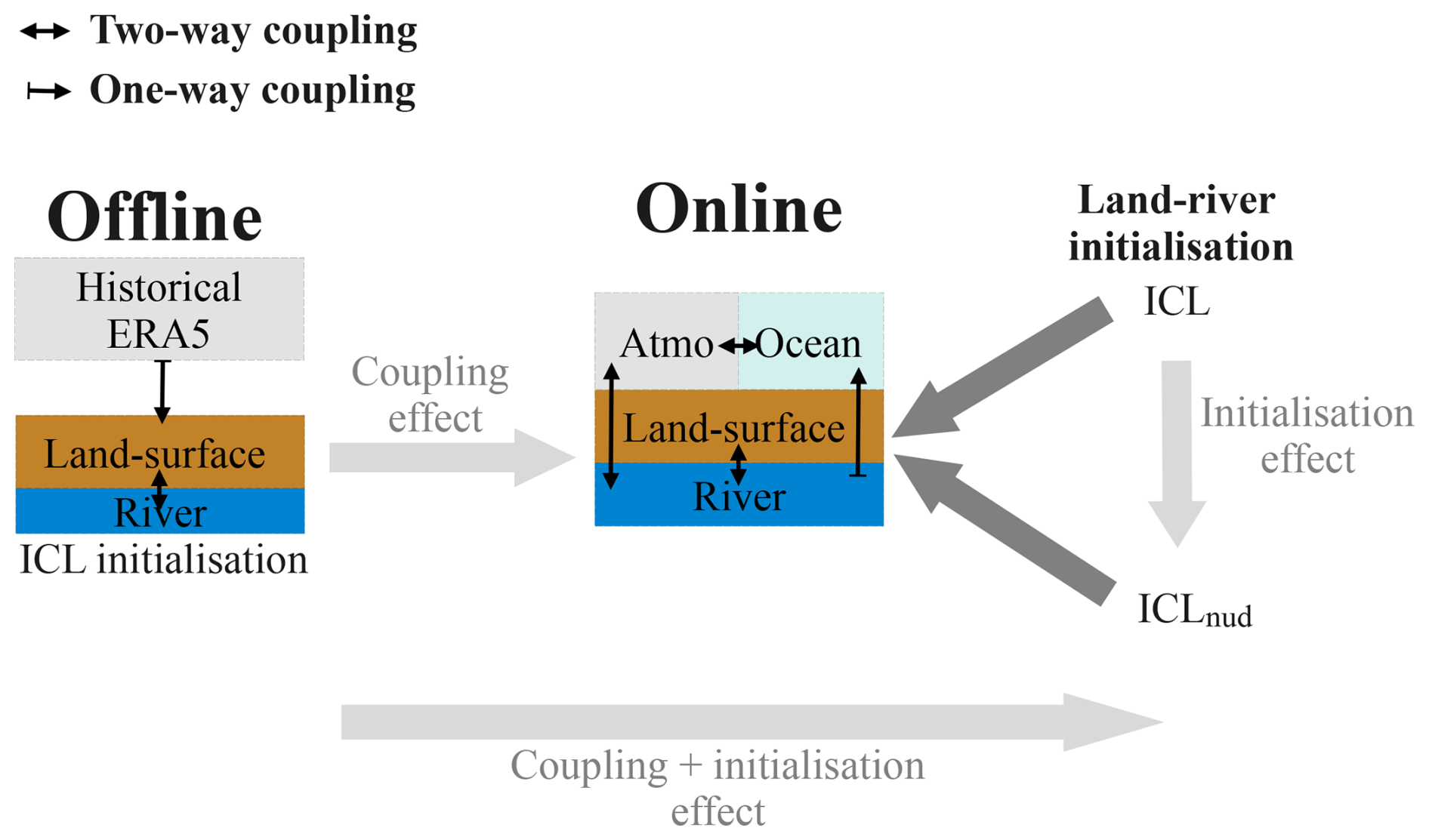
Figure 1 Schematic of offline and online forecast system configurations and corresponding land–river initializations. ICL: initial condition from the historical run with the online system; ICL_nud: initial conditions from a historical run with soil moisture nudged to fields reconstructed from the offline land simulation SMR. As illustrated by the grey-filled arrows, the design of the experiment allows for the evaluation of the coupling effect, the initialization effect or both.

Table 1 Experiments configurations for land initial conditions and hindcast production (see Fig. 1).

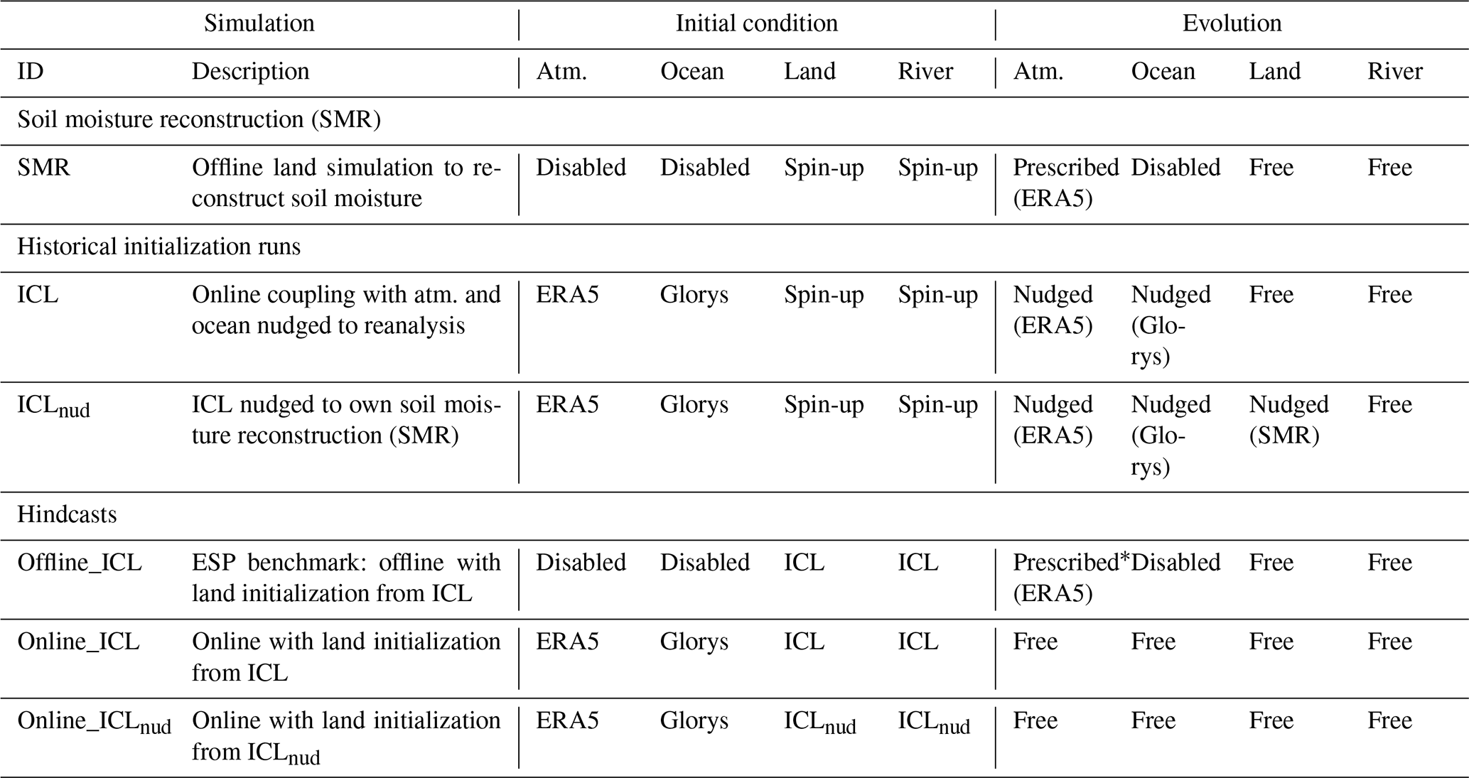
^* The atmospheric ensemble forcing for the Offline_ICL hindcast is constructed from past climate years selected by a leave-3-years-out cross-validation procedure.

To generate the benchmark hindcast Offline_ICL, the land–river model ISBA-CTRIP is forced by ERA5 historical climate (Fig. 1) so that each year produces 1 of the 25 atmospheric forecast members. We use the leave-3-years-out cross-validation (L3OCV) to select the forcing. In L3OCV, the year of the climate forcing cannot match the hindcast year or the preceding year and the two following years to avoid artificially inflating the skill due to large-scale climate–streamflow dependence, with influences lasting from seasons to years, like the North Atlantic Oscillation (Dunstone et al., 2016). For example, to apply the L3OCV selection method to the hindcast of 1993, forcing of the years 1991 and 1996–2019 ensures 25 members. For the hindcast of 2000, forcing from 1991 to 1998 and from 2003 to 2019 is used.

Before computing the forecast performance scores, the daily streamflow is averaged on a 3-month basis to represent the seasonal mean. The 3-month streamflow mean (JJA and DJF) is assessed across a global dataset of gauged basins with the observational streamflow data described in Sect. 2.3. To localize the gauging stations in the correct grid pixel of the model river network, we applied an in-house methodology based on a distance and drainage area station-to-pixel comparison (see Munier and Decharme, 2022, for more details and applications).

2.3 Streamflow observational database

Most previous works evaluate the “potential” streamflow predictability of a forecast system by adopting the perfect-model assumption, in which the streamflow forecast is compared to simulated streamflow (from a model driven by meteorological observations) instead of observed streamflow. Here, we compare the forecasts against observations because, in addition to the IHC and FSC, these incorporate the uncertainty associated with model error (due to structure, physics, and parameter uncertainty) and provides actual (as opposed to potential) streamflow predictability, which is more valuable for end-users or the development of climate services. A database of 1755 flow gauge stations has been created, compiling the global streamflow open-access datasets presented in Table 2. We have filtered the full dataset to remove stations with relatively small drainage areas poorly represented by the model resolution and those stations with more than 25 % of missing streamflow records in the season of concern.

Henck et al. (2011)

Table 2 Streamflow observed datasets.

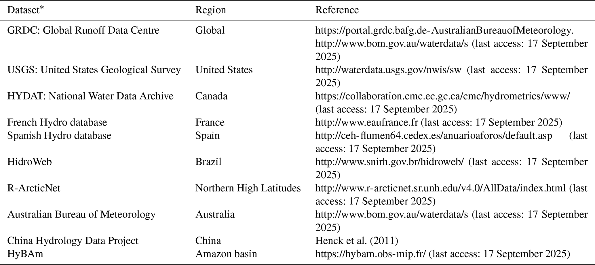
^* In the case of overlapping stations with the global GRDC dataset, priority is given to the national database.

We conducted a correlation analysis to select the minimum drainage area considered in the study. For basins with an area higher than a certain threshold (A_threshold), Fig. 2 shows the correlation between the basin area (A_basin) and the area estimated for the CTRIP routing model (A_CTRIP). With increasing A_threshold, the correlation increases, but the number of available basins is reduced. The threshold is set to 6×10³ km² (about two CTRIP cells per basin in mid-latitudes) to maintain a balance between the number of basins analysed and their geometrical representation and to avoid considering basins inside the spurious oscillating correlation curve (Fig. 2). There are 1451 gauged basins with A_basin≥A_threshold, with an A_basin|A_CTRIP correlation of 0.9886.

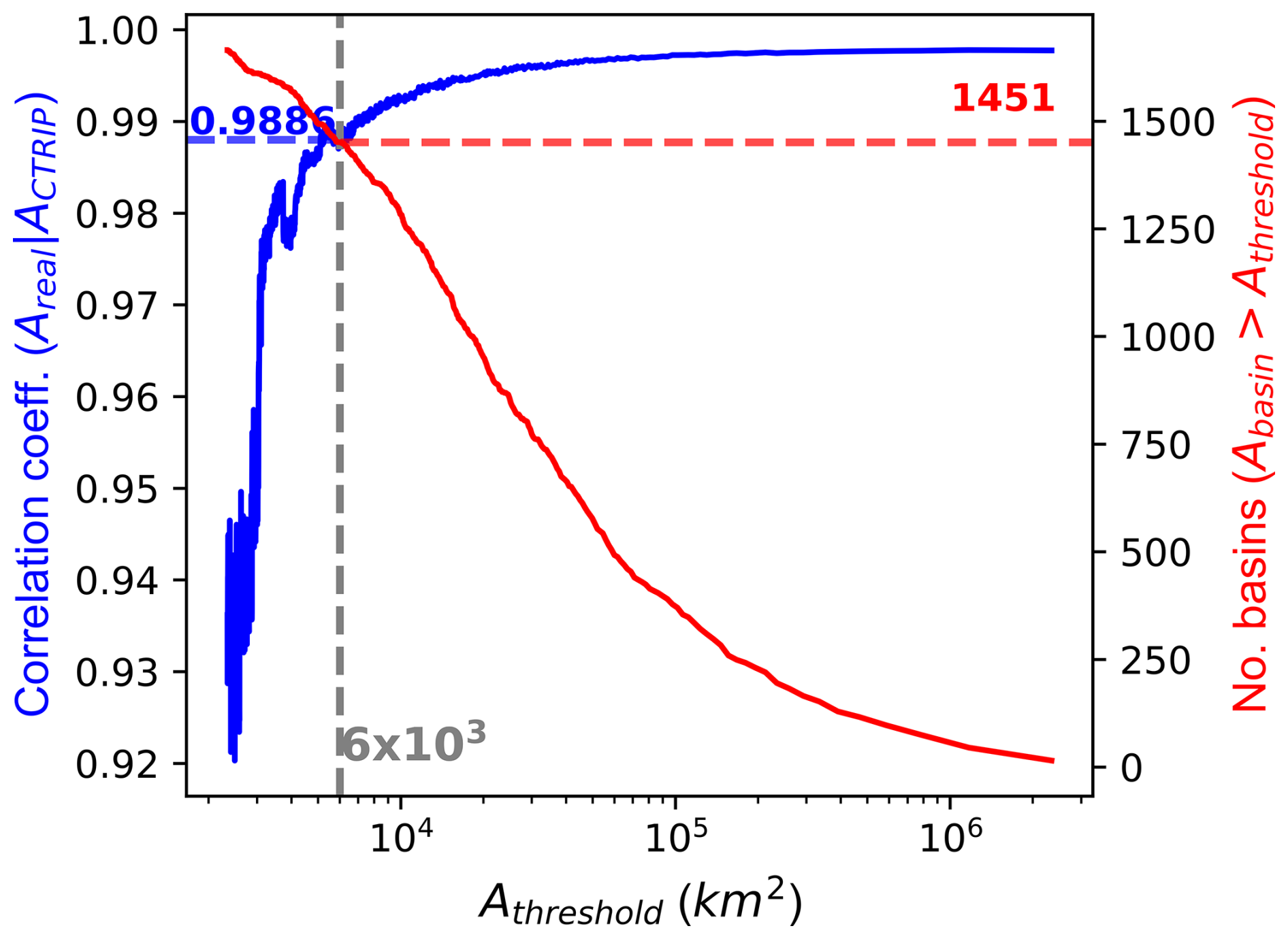
Figure 2 Correlation coefficient of A_real|A_CTRIP and number of basins with an area greater than a given A_threshold.

From the 1451 streamflow stations, we only consider those with less missing data than 25 % of the total data in the analysed season. Figure S1 in the Supplement shows the distribution, in terms of space and frequency, of the full database and the selected stations. The final dataset has 1071 stations in JJA and 1043 stations in DJF, distributed across North America (≈82 %), Europe (≈13 %), South America (3.5 %), Africa (1.7 %), Asia and Australia (0.4 % = 4 stations). In Sect. 3.3, we remove 14 stations where the mean bias magnitude exceeded the maximum machine number in double precision. This can occur in basin outlets, where backflow or strong regulation can lead to a near-zero mean or standard deviation of observed streamflow (in the denominator of bias, the simulated-to-observed mean and standard deviation ratios, as shown in Table 3).

2.4 Streamflow bias correction

Typically, statistical post-processing methods are applied to compensate for errors in model structure or initial conditions, correct biases, and improve ensemble dispersion (Troin et al., 2021). Such bias correction can be applied to atmospheric forecasts (such as precipitation, temperature and evaporation) and/or to hydrological forecasts like runoff and streamflow (e.g. Petry et al., 2023; Tiwari et al., 2022; Gubler et al., 2020; Crochemore et al., 2016; Wood and Schaake, 2008). Our study uses an online atmosphere–ocean–land–river coupled model, for which bias correcting the atmospheric forcing is irrelevant. Instead, we correct the streamflow forecast bias for each flow gauge station using the empirical quantile mapping (EQM) method. To ensure consistent comparisons, we apply streamflow bias correction to both offline and online forecasts.

Unlike adjusting parametric distributions, the EQM method removes bias using empirical cumulative distribution functions (ECDFs) from observations and forecast percentiles. Roughly, the approach replaces the forecast values with observed values corresponding to the same non-exceedance probability (i.e. it calibrates the forecast distribution with the observed distribution by fitting the forecast values). Analogous to Tiwari et al. (2022), the bias-corrected streamflow Q_c is calculated as follows:

$$\begin{array}{}\text{(1)}& Q_{\mathrm{c}}=F_{\mathrm{o}}^{-\mathrm{1}}\left[F_{\mathrm{f}}\left(Q_{\mathrm{f}}\right)\right],\end{array}$$

where F_f and F_o are the ECDFs of forecast Q_f and observation streamflow Q_o, respectively.

2.5 Seasonal forecast assessment

Table 3 presents the deterministic and probabilistic scores used to evaluate the new forecast system performance. The thresholds for the Brier score computation are based on the 3-month average of observed streamflow exceeded 66 % (the lower tercile Q₆₆), 95 % (Q₉₅) and 10 % (Q₁₀) of the time. These thresholds characterize low, very low and high flows (Liu et al., 2021). The skill of the online approach is relative to the performance of the Offline_ICL benchmark.

The significance of the precipitation correlation is calculated using the parametric Student's t test. All other significance tests and confidence interval computations use the bootstrap approach, where 1000 random sub-samples are created from the full sample to establish the probability distribution of the statistical estimator being analysed (e.g. the anomaly correlation coefficient or the Kling–Gupta efficiency (KGE) score). An estimator is considered to be significant if the p value is less than or equal to 0.05.

Table 3 Performance scores used to assess and compare seasonal streamflow forecasting approaches.

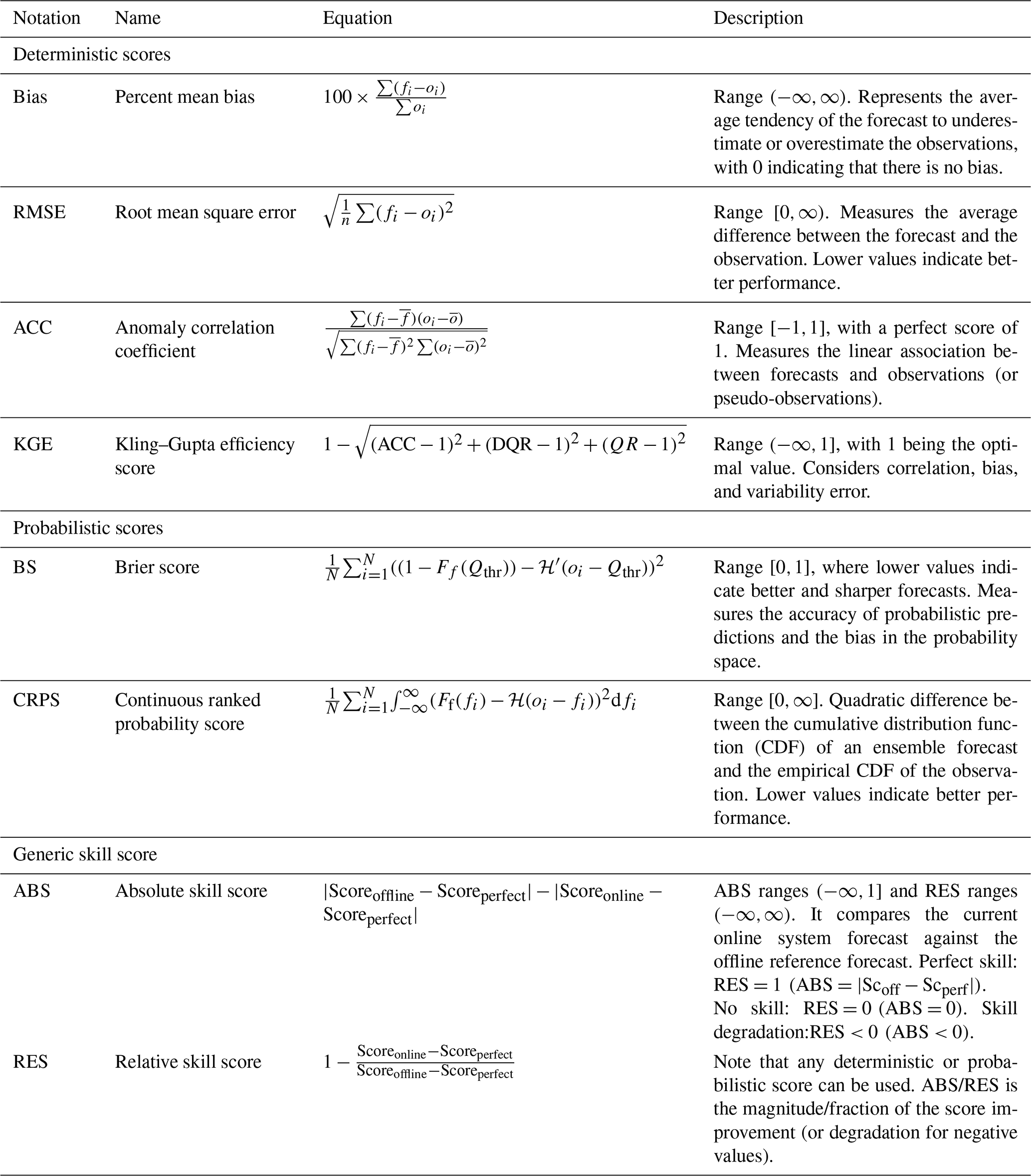
N denotes the total number of forecasts, f_i denotes the forecast 3-month ensemble mean for year i, o_i denotes the observation 3-month mean for year i, $\stackrel{\mathrm{‾}}{f}$ denotes the temporal average over forecast ensemble means, $\stackrel{\mathrm{‾}}{o}$ denotes the temporal average of observations, DQR $=\frac{S_{\mathrm{f}}}{S_{\mathrm{o}}}$ denotes the forecast-to-observation standard deviation ratio, $QR=\frac{\stackrel{\mathrm{‾}}{f}}{\stackrel{\mathrm{‾}}{o}}$ denotes the forecast-to-observation mean ratio, Q_thr is a threshold that represents the occurrence of a hydrological event, the step function ${\mathcal{H}}^{\prime }(o_i-Q_{\mathrm{thr}})$ is zero if o_i≤Q_thr and is 1 otherwise, F_f(f_i) denotes the cumulative distribution function of the ensemble forecast, the Heaviside step function ℋ(o_i−f_i) is zero if f_i<o_i or 1 if f_i≥o_i, Score_offline denotes the score of the Offline_ICL benchmark reference forecast, and Score_perfect is the score of a perfect forecast.

3 Results

The first two sub-sections explore the performance of the two primary factors of hydrologic predictability, namely the initial hydrologic conditions (Sect. 3.1) and the future climate seasonal anomalies (Sect. 3.2). Section 3.3 presents the evaluation of the seasonal prediction skill to highlight the joint and separate impacts of the coupling and the enhanced land initialization.

3.1 Initial hydrologic conditions

We assess the global performance of the river streamflow simulated by the initialization runs (ICL and ICL_nud) against historical streamflow observations. For this purpose, we compare the initial-month mean streamflow (May for JJA and November for DJF) against the observed streamflow over the 1993–2017 period.

Figure 3 presents three performance metrics of the comparison (bias, root mean square error and anomaly correlation coefficient). Note that only stations with less than 25 % of missing data during the corresponding month are considered in the following analysis.

For May, the streamflow bias of the ICL tends to be positive in the driest regions (Fig. 3a), particularly in the west of North America, northeastern Brazil, southern Africa, the Iberian Peninsula and Australia. The higher concentration of red markers in Fig. 3b suggests a reduction in bias from the ICL to ICL_nud. This reduction is more pronounced for negative bias, as indicated by the shift of the negative peak towards zero bias in the frequency distribution shown in Fig. 3c. Besides this, the RMSE is generally smaller with ICL_nud, particularly over regions with large RMSEs in the ICL (Fig. 3d–f). In seasonal forecasts, the temporal correlation between the forecasted and the observed anomalies is crucial since it indicates the capability of capturing the interannual variability of streamflow departures from the mean value. The spatial distribution of the difference in the anomaly correlation coefficient $\mathrm{|}{\text{ACC}}_{\text{ICL}}-\mathrm{1}\mathrm{|}-\mathrm{|}{\text{ACC}}_{{\text{ICL}}_{\text{nud}}}-\mathrm{1}\mathrm{|}$ in Fig. 3h shows that the soil moisture nudging improves the temporal dynamics of the simulated streamflow in May over most of the 1067 gauging stations. The result is verified in Fig. 3i, which reports up to 20 % more stations with $\mathrm{ACC}>(\mathrm{0.4}-\mathrm{0.6})$.

The performance of the river initialization in November (used for DJF forecasts) is presented in Fig. S3. ICL_nud tends to reduce the mean bias of stations displaying a high positive bias in the ICL (Fig. S3a–b). The global distribution of bias in Fig. S3c confirms a reduction in high positive bias, favouring the concentration of bias values closer to zero than in the ICL. However, unlike in JJA, in DJF, ICL_nud enhances the number of basins with higher RMSE and lower ACC. In Sect. 3.3, we show and discuss the impact of the initial hydrologic condition (IHC) degradation on the hindcasts in boreal winter.

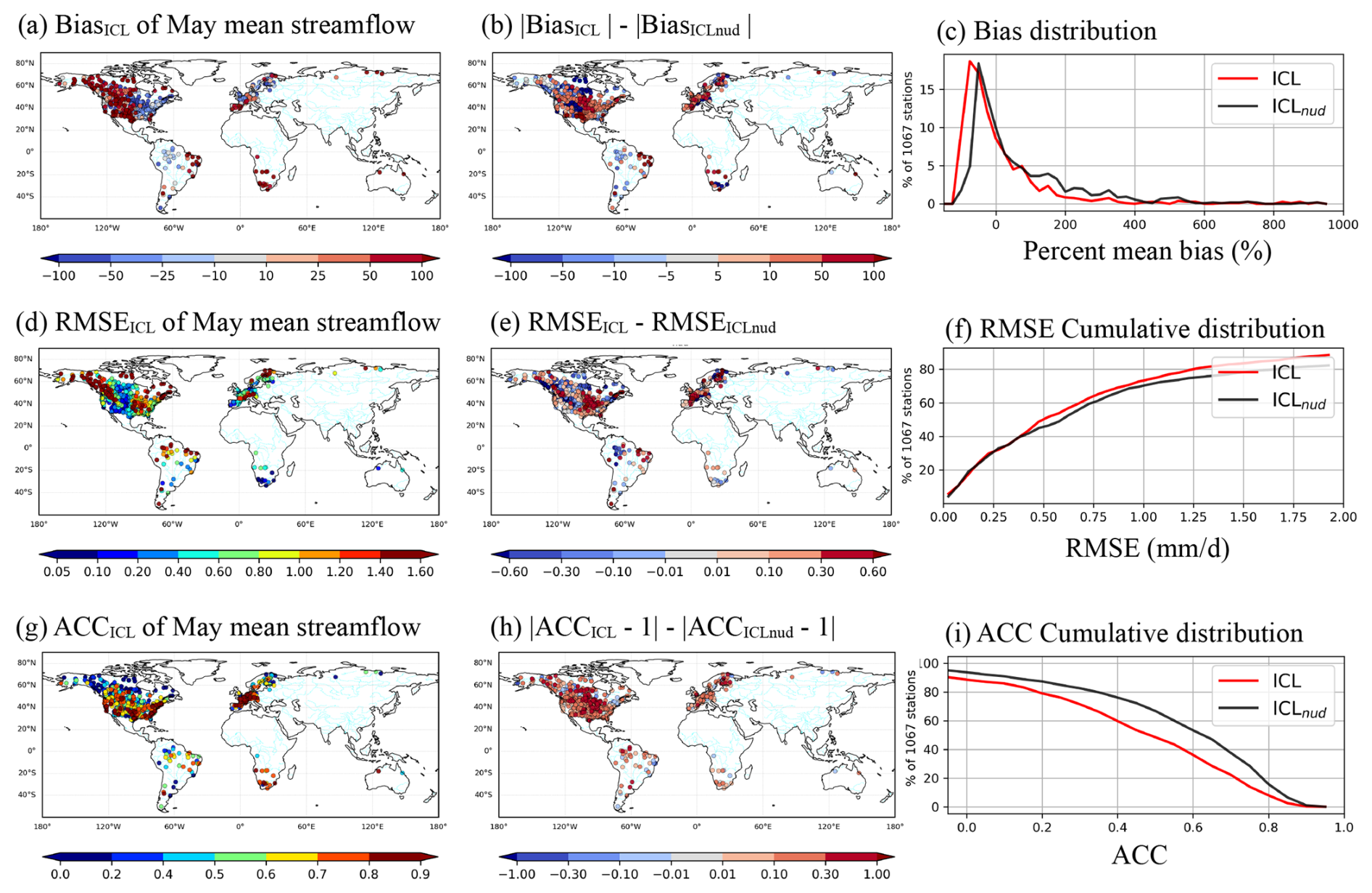
Figure 3 Comparison between May streamflow mean of initialization run against the observed streamflow over 1993–2017. Left column: ICL bias (a), root mean square error (mm d⁻¹) (d) and anomaly correlation (g). Middle column: difference with the ICL_nud enhanced land initialization bias (b), root mean square error (mm d⁻¹) (e) and anomaly correlation (h). Right column: distribution of bias for each experiment (c), accumulated distributions of the root mean square (f) and anomaly correlation (i).

3.2 Precipitation and temperature skill

One way to bring out the influence of the land–atmosphere coupling is to assess the impact of different land IHCs on the atmospheric forecast. The performance of the atmospheric seasonal forecast is presented in Figs. 4 and 5, particularly for two of the most important water cycle drivers: precipitation and near-surface temperature. Precipitation is compared against the Multi-Source Weighted-Ensemble Precipitation (MSWEP v2, Beck et al., 2019), and the temperature is compared against the Climatic Research Unit gridded Time Series (CRU TS v4.05, Harris et al., 2020).

A global view does not reveal marked changes in terms of ACC for the atmospheric predictions. However, from a continental to regional scale, differences are noticeable. In boreal summer (Fig. 4), enhanced initialization ICL_nud tends to increase precipitation correlation in the middle region of South America, including the Paraná River basin and the southern Amazon basin (red box), with degradation in the northeast of Brazil, Australia, and some areas of North America and Asia north of 40 ° N (cyan boxes). Notably, Europe experiences improved precipitation predictions. Temperature predictions are less sensitive to the land initialization in summer, but degradation is concentrated in higher latitudes (north of 40° N and south of 20° S). In winter, regions with reduced performance for both precipitation and temperature predictions are primarily found in North Africa, Europe and Asia (Fig. 5).

We have found that the ICL_nud initialization can have a detrimental effect on the accuracy of precipitation and temperature seasonal forecasts. This is due to soil moisture nudging, a technique intended to enhance the variability of soil water content and to improve the forecast of river streamflows. However, it can also lead to adverse effects on the land–atmosphere coupling simulated by the model. The initial soil moisture conditions introduced by the offline nudging technique may shift the coupled system away from its equilibrium state. When the forecast integration begins, the nudging constraint is deactivated, and the model is adjusted to its equilibrium, potentially generating misleading heat and water fluxes at the land–atmosphere interface. This could ultimately disrupt the atmospheric circulation and reduce the accuracy of the temperature and precipitation forecasts.

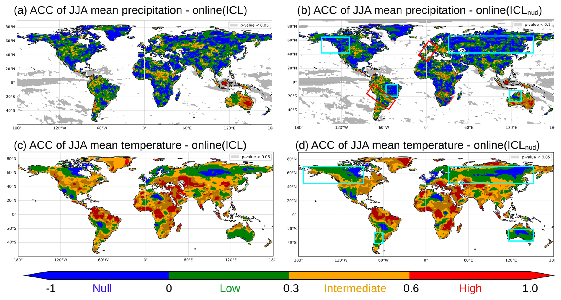
Figure 4 Comparison of Online_ICL and Online_ICL_nud atmospheric forecasts for the anomaly correlation coefficient of the JJA 3-month mean precipitation (a, b) and temperature (c, d). Red (cyan) boxes highlight regions with a noticeable ACC increase (decrease).

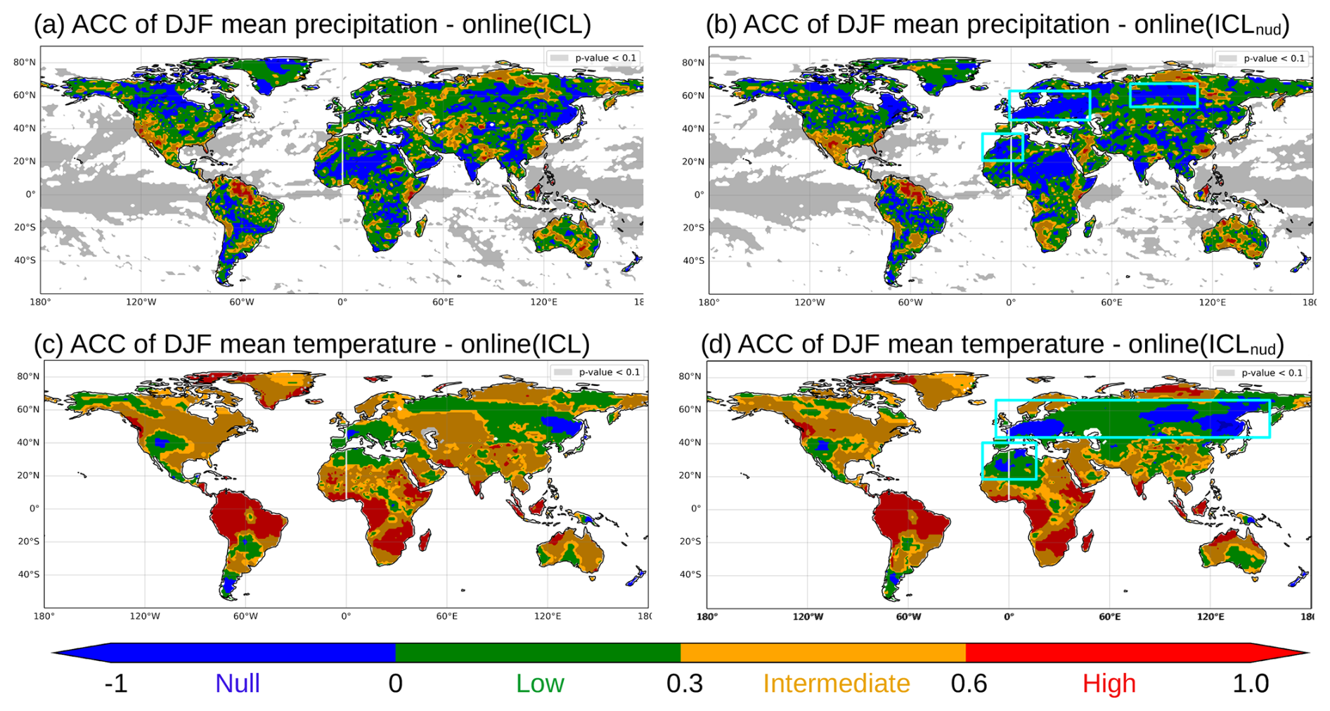
Figure 5 Comparison of Online_ICL and Online_ICL_nud atmospheric forecasts for the anomaly correlation coefficient of the DJF 3-month mean precipitation (a, b) and temperature (c, d). Red (cyan) boxes highlight regions with a noticeable ACC increase (decrease).

We have shown evidence of the impact of land IHC on the performance of seasonal atmospheric forecasts as proof of the importance of land–atmosphere feedback. In the following section, we will explore the sensitivity of the SSF to enhanced IHCs in a fully coupled global forecast system.

3.3 Impact of initialization and coupling on streamflow forecast skill

The hindcast performance of the ESP benchmark (Offline_ICL) is compared against the hindcasts of the fully coupled configurations with two different land initializations (Online_ICL and Online_ICL_nud) to determine the contributions of initialization and land–atmosphere coupling. Unlike online configurations, where the model forecasts the atmosphere, in Offline_ICL, the atmosphere forcing is based on climatology without land–atmosphere feedback. More details on the three configurations can be found in Sect. 2.2.2.

3.3.1 Global view

In boreal summer, the spatial distribution of the anomaly correlation coefficient of the hindcasts compared to the benchmark Offline_ICL reveals a limited effect of the coupling Online_ICL (Fig. 6a–b). However, a substantial improvement in the JJA streamflow forecast is achieved with the enhanced initialization Online_ICL_nud (Fig. 6c), also drawn by the cumulative distribution in Fig. 6d.

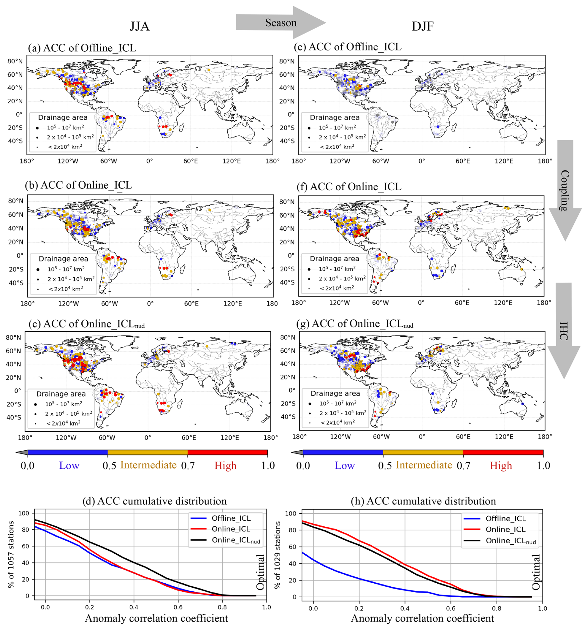
Figure 6 Anomaly correlation coefficients (ACCs) of bias-corrected streamflow hindcasts computed against observations in JJA (first column) and DJF (second column). Offline_ICL benchmark (first row) and the online coupled configurations with conventional initialization (second row) and improved initialization (third row). Cumulative distribution of the anomaly correlation coefficient of the corresponding season (last row). Markers with transparency represent stations with a statistically non-significant ACC at the 95 % confidence level.

For winter, in the second column of Fig. 6, the coupled hindcasts with both land initializations yield a remarkable increase in stations with intermediate and high correlation. The cumulative distribution of the ACC, in Fig. 6d, confirms that the number of stations with an ACC greater than 0.5 (0.7) increases to more than 25 % (7 %). In addition, from Online_ICL  to Online_ICL_nud, the ACC is slightly reduced, especially for basin outlets to the north of 40° N. This suggests that soil moisture nudging in ICL_nud tends to reduce the ability of the system to predict winter streamflow dynamics in basins with strong ice influence. It should be pointed out that a monthly analysis of the performance at different lead times, presented in Fig. S5, shows the same conclusions as the 3-month mean analysis in Fig. 6d–h.

A global view of the impact of bias correction, coupling and enhanced initialization is presented in Fig. 7. For the three models set up, the cumulative distributions of ACC and KGE are computed for the raw and bias-corrected hindcasts for the boreal summer (JJA) and winter (DJF) seasons. Before and after bias correction, both online hindcasts outperformed the offline configuration. Furthermore, both metrics confirm that the hindcast skill with the enhanced initial condition ICL_nud is improved compared to Online_ICL in summer but worsened slightly in winter. As expected, the ACC was weakly modified after bias correction (Fig. 7a against b), while the number of stations with positive KGE values increased up to 20 %, except the Offline_ICL, which was less sensitive to the bias correction in DJF (Fig. 7c against d). This means that the biggest contribution of bias correction comes from the forecasted-to-observed streamflow mean and standard deviation ratio.

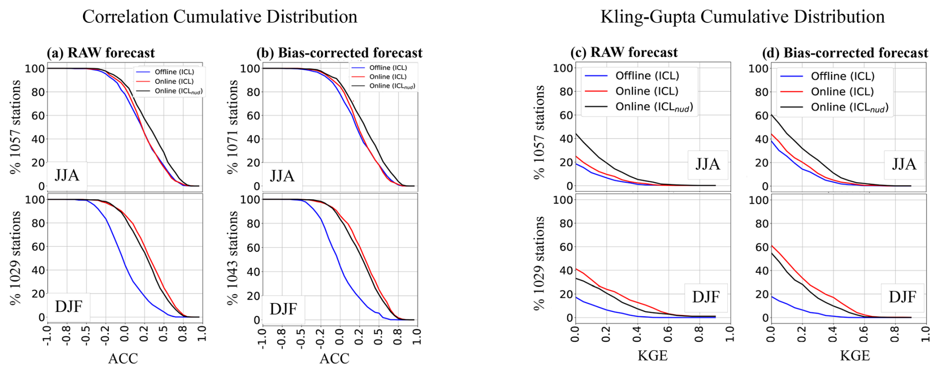
Figure 7 Cumulative global distributions of anomaly correlation coefficient (a, b) and Kling–Gupta efficiency score (c, d) of raw (a, c) and bias-corrected (b, d) forecasts.

Figure 8 displays the deterministic and probabilistic scores as a function of the basin area. For all JJA streamflow predictions, the KGE (and its component scores in Fig. 8a) and the CRPS (continuous ranked probability score) (Fig. 8b) reveal an improvement with increasing drainage area, while low, mean and high flow predictions (BS95, BS66 and BS10) report weak basin area dependence. The figure confirms that Online_ICL_nud outperforms Online_ICL for both deterministic and probabilistic metrics. Unlike Offline_ICL, the median scores of coupled systems show weak to null dependence on basin area in winter, while the amplitude of the variation decreases with the area (Fig. 8c and d). Besides, in winter, the Offline_ICL produces poor-quality forecasts in most gauge stations, as reported by the low median KGE and ACC values. However, for basins with a drainage area ≥10⁶ km², the Offline_ICL is close to Online_ICL and Online_ICL_nud. It should be noted that Online_ICL_nud has a negative impact in winter, reducing the mean forecast performance for the basin area ranges in terms of variability (ACC in Fig. 6) and oscillation amplitude ($\frac{S_{\mathrm{f}}}{S_{\mathrm{o}}}$: forecast-to-observation deviation ratio in Fig. 8c).

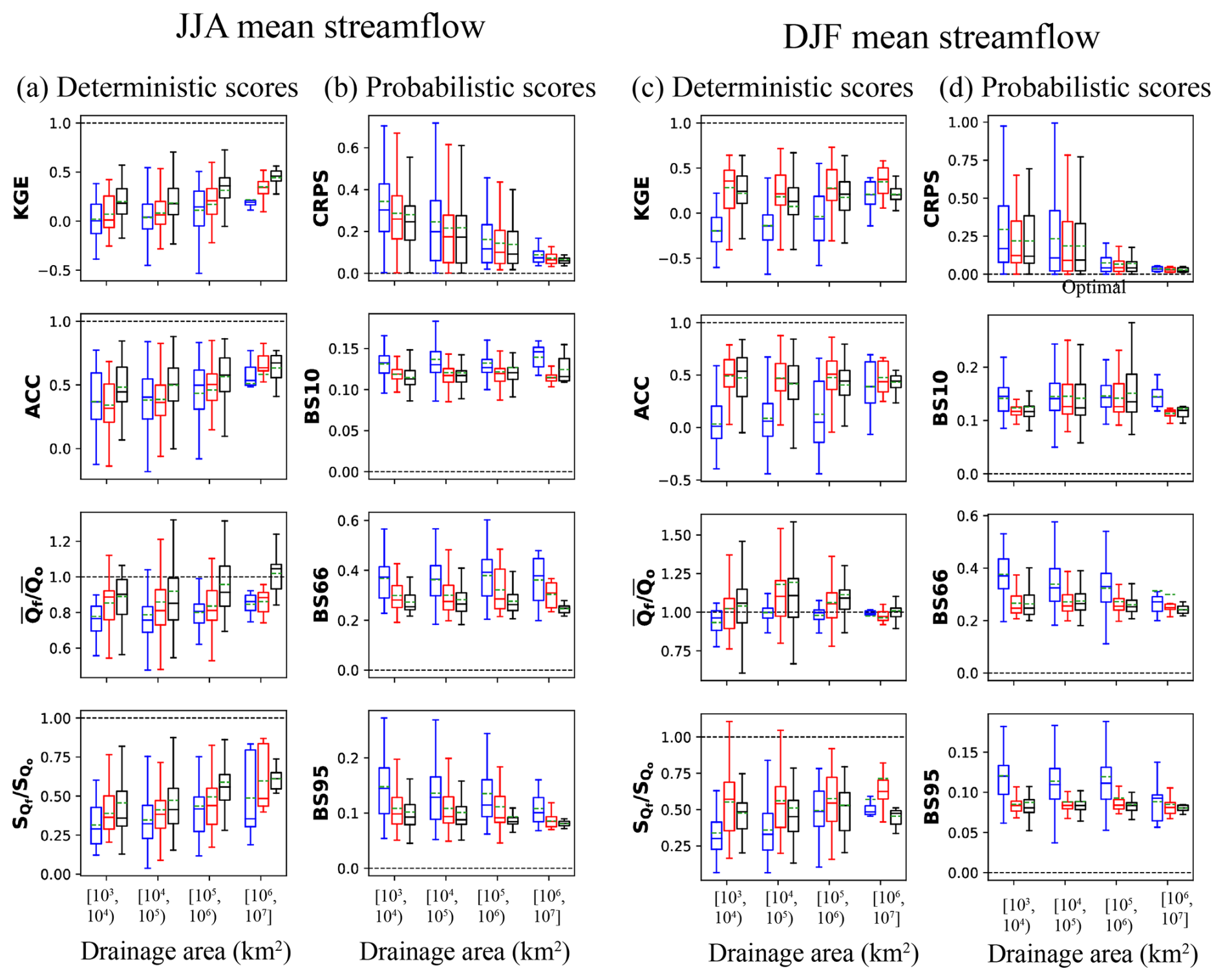
Figure 8 Performance of the hindcast 3-month mean streamflow as a function of the basin area for summer (two left columns) and winter (two right columns). Scores computed in all gauging stations of the global database are visualized in boxplots of deterministic (a, c) and probabilistic (b, d) scores. Four basin area classes are defined, with 131, 670, 215 and 41 stations for JJA and 123, 656, 210 and 40 stations for DJF. The colour of the box represents the model configuration: blue denotes Offline_ICL, red denotes Online_ICL, and black denotes Online_ICL_nud. The horizontal dashed black lines delimit the optimal value of the corresponding metric. The continuous line in the box is the median, while the dashed green line indicates the mean value.

The density, quantity and distribution of the flow gauge stations vary significantly between continents. As shown in Fig. 6d, the distribution of the scores in the frequency space tends to reflect the continent with more gauge stations, such as North America, in this case. Therefore, in the next section, we will assess the forecast performance on a continental scale.

3.3.2 Continental scale

Figures 9 and 10 present the KGE spatial and frequency distribution for summer and winter in North America, Europe, South America and Africa. In summer, on the seasonal timescale, the river discharge tends to be driven by water released from the basin water storage. Consequently, the initialization of the soil water content (soil moisture) of the land component plays a major role in streamflow prediction. This applies to North America and Europe, where enhanced land initialization has a more positive impact than atmospheric coupling with conventional initialization. Meanwhile, in winter, streamflow is primarily driven by precipitation. This means that rainfall forecasts matter more than water content and land initialization quality. The cumulative KGE distribution of Fig. 9 confirms that, independently of the initialization, the atmospheric forecast coupled with land yields improved predictions with respect to the Offline_ICL.

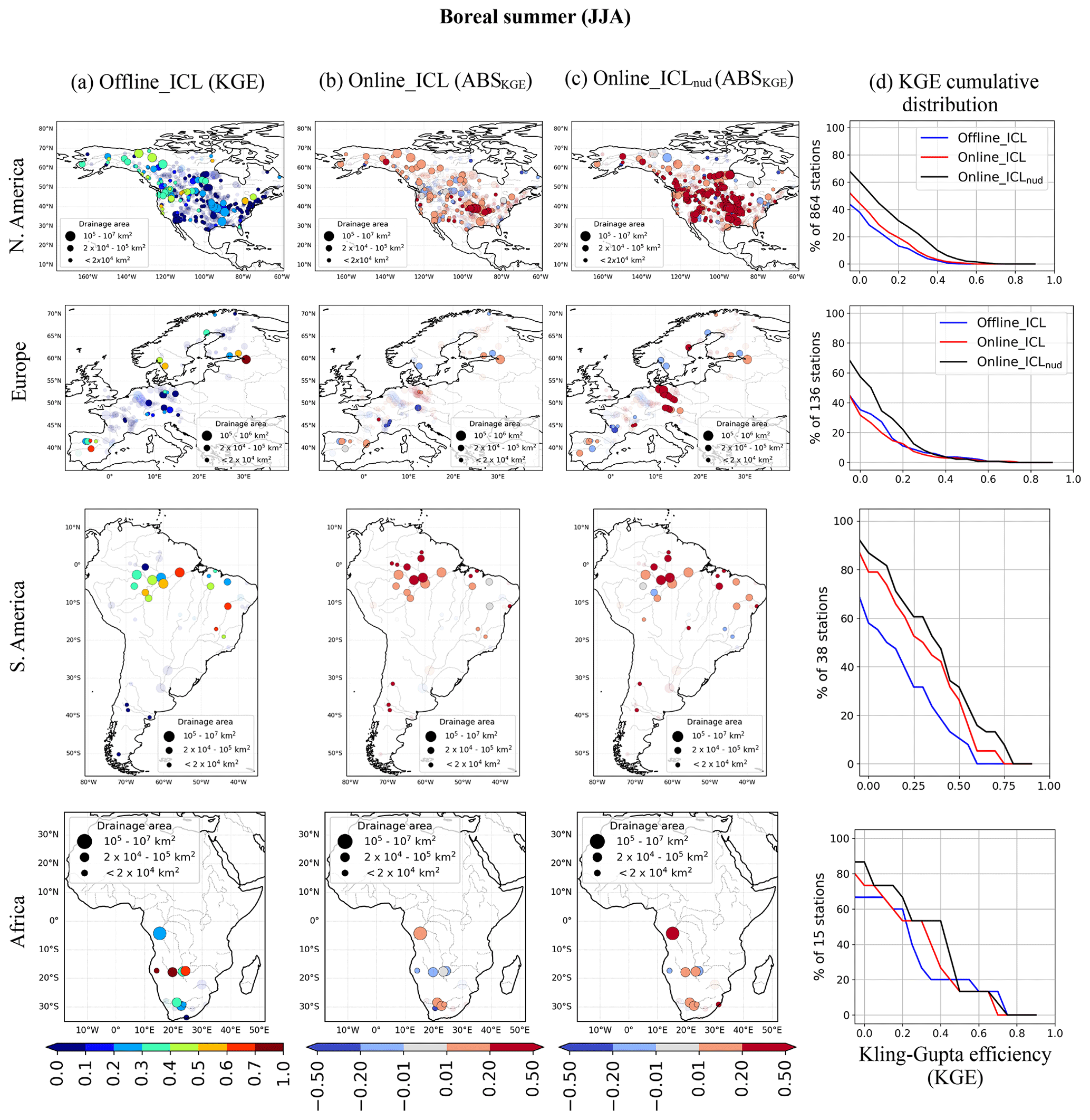
Figure 9 Comparison of seasonal streamflow hindcasts performance in boreal summer JJA. The maps display the station-wise KGEs for the seasonal streamflow of the (a) Offline_ICL hindcast and the absolute skill score of (b) Online_ICL and (c) Online_ICL_nud experiments. Column (d) exhibits the three KGE cumulative distributions for the corresponding continent. Markers with transparency represent stations where KGE is significantly negative, with a confidence of 95 %.

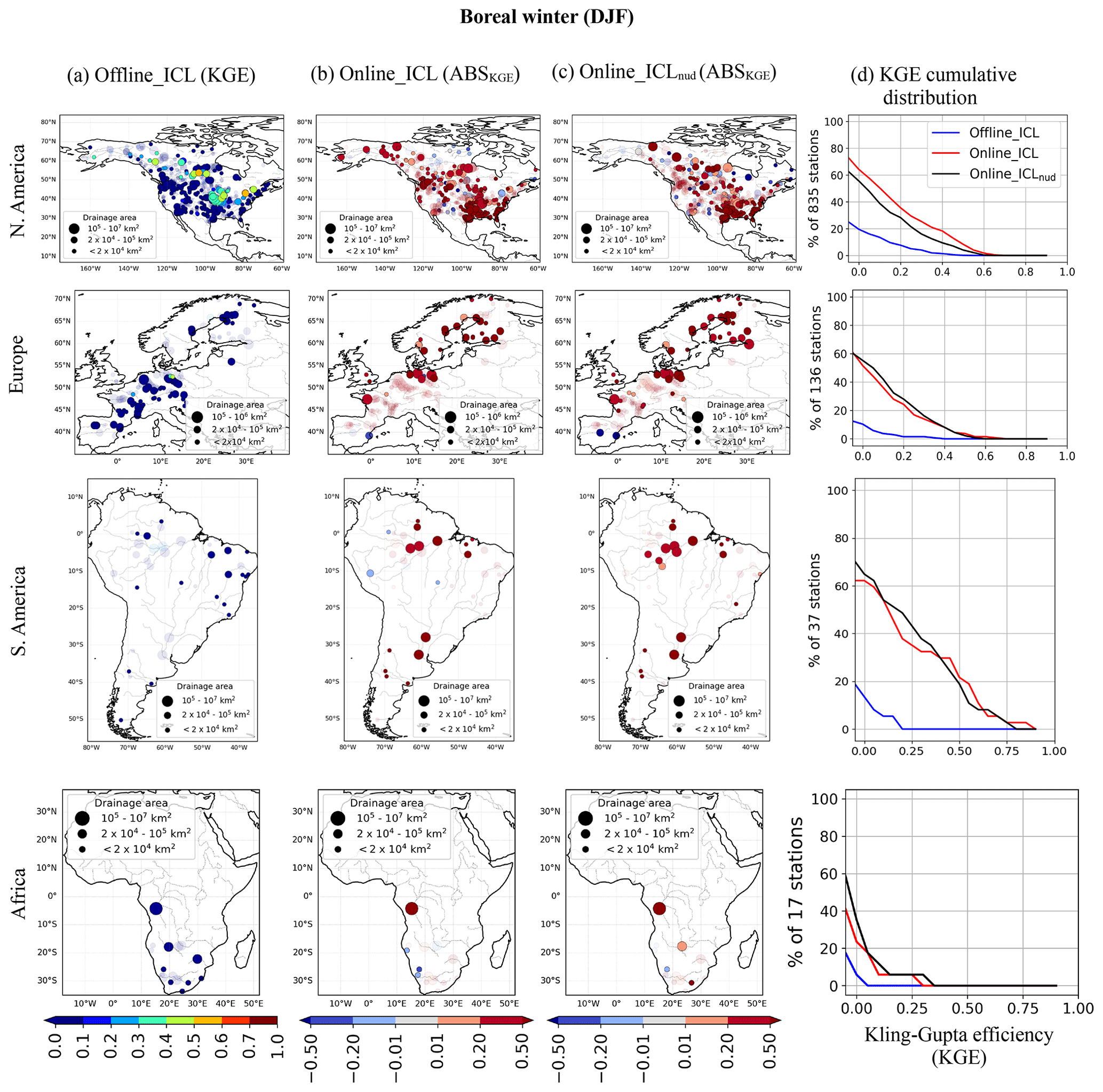
Figure 10 KGEs for the streamflow in boreal winter of the (a) Offline_ICL hindcast and the absolute skill score of (b) Online_ICL and (c) Online_ICL_nud experiments. (d) KGE cumulative distributions for the corresponding continent. Markers with transparency represent stations where KGE is significantly negative, with a confidence of 95 %.

The greatest improvement in South American rivers for both seasons comes from the dynamic atmospheric forecast incorporated into the coupled systems. Due to the few gauge stations in Africa, the cumulative distribution does not provide robust information. As a result, the different levels of coupling and initialization do not show evidence of the impact on the seasonal prediction of streamflow in the 15–17 gauging stations evaluated in Africa. Besides, most of the (few) gauges in Africa are in the southern part of the continent, where JJA is the dry season, while DJF is positioned in the (monsoonal) wet season. Under this data availability context for Africa, all the model setups provide satisfactory predictions in the dry season (JJA), while they perform poorly during the wetter monsoonal summer season (DJF).

Before advancing in the skill analysis, we have identified basins exhibiting pertinent accuracy for the hindcasts, whereby at least one of the three hindcast configurations yields a significant positive anomaly correlation coefficient (indicated by the lower 95 % confidence bound of the ACC being negative). This screening retains 650 stations in JJA and 620 in DJF (Fig. S2), presenting a distribution of drainage areas, as depicted in the initial data (Fig. S1), predominantly skewed towards values below 2×10⁵ km², with a substantial number of basins exceeding 10⁶ km² in area.

In addition to the ACCs for the comprehensive dataset in Fig. 6, Fig. S4 presents the ACC map of the benchmark alongside the absolute skill score of online configurations after the exclusion of stations exhibiting negative correlation hindcasts across all configurations.

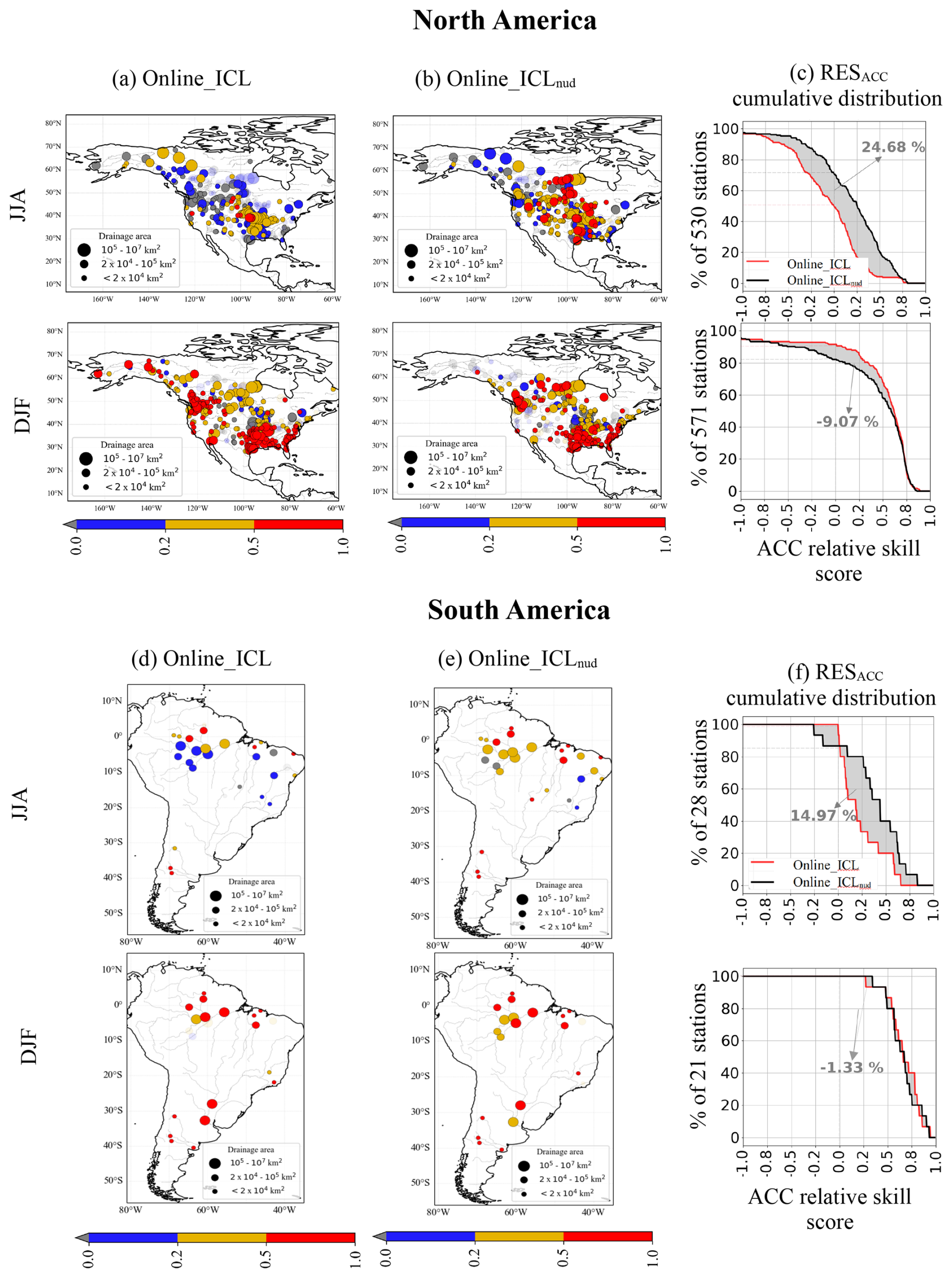
Figure 11 Comparison of online hindcasts with respect to the offline benchmark reference in North America (a–c) and South America (d–f). The relative skill score RES of anomaly correlation is $\mathrm{1}-({\mathrm{ACC}}_{\text{online}}-\mathrm{1})/({\mathrm{ACC}}_{\text{offline}}-\mathrm{1})$. In each panel, the two left columns present the RES map, and the right column presents its cumulative distribution for summer (first row) and winter (second row). The grey area between cumulative distribution curves is the percentage of ACC skill added by the new initialization in relation to the conventional one (negative values indicate skill degradation).

The correlation relative skill of online approaches with different initializations compared to the Offline_ICL, defined as $\mathrm{1}-({\mathrm{ACC}}_{\text{online}}-\mathrm{1})/({\mathrm{ACC}}_{\text{Offline\_ICL}}-\mathrm{1})$, is presented in the maps and cumulative distributions of Fig. 11. During summer, in North America (Fig. 11a–b), the enhanced initialization provides about 25 % additional skill (Fig. 11c). However, in winter, it degrades the forecast, mainly at latitudes >60° N (Fig. 11d–e), by about 9 % (Fig. 11f). In South America, the ACC skill increases in summer by about 15 % because of the initialization, while, in winter, it yields a slight degradation close to 1 %.

To summarize the SYS8 assessment, the relative skill of online approaches is presented for three deterministic and four probabilistic scores in Fig. 12. A positive relative skill score indicates an improvement with respect to Offline_ICL, where 1 corresponds to the perfect score. For example, in the North American winter season, the median ACC is 45 % (for Online_ICL) and 38 % (for Online_ICL_nud) closer to the perfect correlation than Offline_ICL. For boreal summer (top row of Fig. 12), all skill metrics confirm the added value of enhanced land initialization ICL_nud in improving streamflow forecasts. However, over South America and Africa, the probabilistic metrics show more elusive improvement (or degradation). For boreal winter (bottom row of Fig. 12), forecasts show higher performance than the benchmark in general but suggest a minor impact of improved land initial conditions. The deterministic scores also reveal that the skill gain for online approaches is sharper for ACC than RMSE and KGE, which denotes a better ability of coupled forecast systems to capture the interannual variability of river streamflows. In JJA and DJF, the reduction in RMSE, if any, remains limited for most continents. Additionally, the Brier skill score for high flows (BS10) is generally lower than BS66 and BS95 for mean and low flows. This result suggests either that the forecast systems anticipate better seasonal droughts than excessive cumulated precipitation or that dry initial conditions, associated with low flows, are more persistent than the wet counterpart.

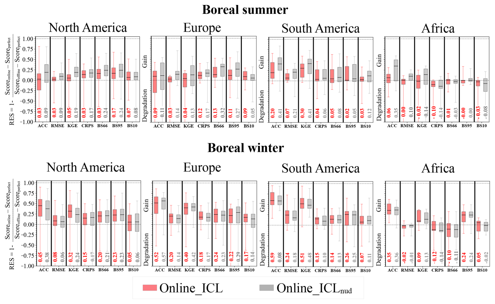
Figure 12 Distribution of relative skill metrics of Online_ICL (red boxplots) and Online_ICL_nud (grey boxplots) with respect to the benchmark Offline_ICL for each continent in JJA (top row) and DJF (bottom row). Coloured numbers indicate the mean values.

3.4 When, where and why the SYS8 is skilful

The enhanced land–river initialization was designed to capture the spatial and temporal dynamics of soil moisture and thus improve water storage variation. For this purpose, soil moisture is nudged to reconstructed fields of a reanalysis based on a surface model driven by ERA5 atmospheric forcing.

In boreal summer, enhanced land initialization is more critical than using a fully coupled GCM-derived forecast system since only the former approach led to improved forecasts. For this season, the highest impact of initialization on forecast skill occurs in large basins of the driest regions, where streamflow is strongly sustained by the water storage naturally released during low flows (i.e. baseflow).

In boreal winter, the new IHC negatively affected basins at high latitudes, probably due to the potential disruption of the energy, ice and liquid water budget in the soil induced by the lack of nudging of soil temperature (e.g. Ardilouze and Boone, 2024), which could lead to spurious model adjustment through excessive or reduced runoff. Confirming this would deserve a dedicated evaluation beyond the scope of this study. In South America, the coupling is beneficial (for both IHCs) in JJA and DJF, which is consistent and directly related to the strong ACC of precipitation and temperature provided by the online systems in most of the basins analysed in South America (see Figs. 5 and 4). For Africa, no robust conclusions can be drawn from the results due to the reduced sample of stations. Still, predictions from all model configurations in DJF were poor, with fewer than 40 % of stations exhibiting a positive KGE.

4 Conclusions

In this paper, we assess the Météo France global streamflow seasonal forecast operational system (SYS8) based on the latest version of the CNRM global climate model CNRM‐CM6‐1. This model incorporates an advanced river routing model that interacts with the land surface component via surface and sub-surface runoff, unconfined aquifer water exchange and saturated floodplain (re)infiltration and with the atmosphere through free-water evaporation and precipitation interception on floodplains. We thus employ SYS8 to produce a 25-member ensemble of daily streamflow hindcasts extending up to 4 months, with burst initialization on 1 May and 1 November, to predict, respectively, the boreal summer and winter global seasonal streamflow from 1993 to 2017.

The seasonal streamflow anomalies are evaluated against observations to assess the actual skill with respect to a classical ensemble streamflow prediction (ESP) offline approach, used as a benchmark forecast. In addition to assessing the skill of the coupled forecast system, we compare two different land initialization strategies. We found that the seasonal streamflow forecast (SSF) of SYS8 can be skilful during the boreal summer and winter seasons.

The main novelty and conclusions of this work can be condensed into the key points listed below.

• Our results demonstrate, for the first time, the potential to utilize direct global streamflow forecasts issued by a global climate model fully coupled with a river–floodplain model. The convenient single-step workflow natural to the coupled approach employed in SYS8 allows simultaneous production of atmospheric and streamflow forecasts, while the online coupled model ensures consistency in conservation laws at the initialization and during the forecasting.

• In boreal summer, the water storage initialization has the largest positive impact on the SSF quality. The improvement is sharper in the driest regions and for the largest basins, where high storage capacity drives the basin response during low-flow periods typical of summer.

• In boreal winter, the streamflow variability tends to be mostly induced by seasonal precipitation anomalies, thereby reducing the impact of the initialization on the SSF performance. The atmospheric predictive capacity of the coupled model, albeit relatively limited over mid-latitude regions, leads to SSF being more accurate overall than the benchmark ESP offline forecast driven by climatology-based atmospheric forcing.

Current efforts to extend the assessment of the actual skill of SYS8 to other parts of the globe include augmenting the observation database with discharge time series from regional and local flow station datasets. In future work, we will also evaluate the potential predictability of the system using the perfect model approach. In this framework, the river streamflow historical time series derived from the initialization run is used as a verification dataset instead of actual observations. This approach allows us, first, to remove the influence on river discharges of human activity that is not parameterized in the model (dams, reservoirs, irrigation). Secondly, the forecast evaluation can be performed at every location where the model simulates a streamflow. This allows us to define a set of virtual stations equally distributed across the globe and thereby also assess the predictions in regions that are poorly instrumented.

Our study also provides insights for improving the forthcoming generation of forecast systems for hydrological predictions, particularly regarding initialization methods.

In light of our results, we aim to explore other seasons and to develop a novel and more robust land–river initialization with more realistic soil moisture conditions. This strategy is currently being tested via the in-house land data assimilation system LDAS-Monde (Albergel et al., 2020) in the context of the Horizon Europe project CERISE (https://www.cerise-project.eu/, last access: 17 September 2025). Finally, in the longer term, we expect forecast improvement from better representation of the influence of human activity on the terrestrial water cycle. In particular, we will evaluate the activation of the novel irrigation scheme (Decharme et al., 2025) within a higher-resolution version of CTRIP (Munier and Decharme, 2022) in the CNRM-CM GCM of the next generation for CMIP7, focusing on river streamflow seasonal predictions.