What controls the tail behaviour of flood series: rainfall or runoff generation?

Many observed time series of precipitation and streamflow show heavy-tail behaviour. For heavy-tailed distributions, the occurrence of extreme events has a higher probability than for distributions with an exponentially receding tail. If we neglect heavy-tail behaviour we might underestimate the magnitude of rarely observed, high-impact events. Robust estimation of upper-tail behaviour is often hindered by the limited length of observational records. Using long time series and a better understanding of the relevant process controls can help with achieving more robust tail estimations. Here, a simulation-based approach is used to analyse the effect of precipitation and runoff generation characteristics on the upper tail of flood peak distributions. Long, synthetic precipitation time series with different tail behaviour are produced by a stochastic weather generator. These are used to force a conceptual rainfall–runoff model. In addition, catchment characteristics linked to a threshold process in the runoff generation are varied between model runs. We characterize the upper-tail behaviour of the simulated precipitation and discharge time series with the shape parameter of the generalized extreme value (GEV) distribution. Our analysis shows that runoff generation can strongly modulate the tail behaviour of flood peak distributions. In particular, threshold processes in the runoff generation lead to heavier tails. Beyond a certain return period, the influence of catchment processes decreases and the tail of the rainfall distribution asymptotically governs the tail of the flood peak distribution. Beyond which return period this is the case depends on the catchment storage in relation to the mean annual rainfall amount.

1 Introduction

Many observed streamflow and precipitation time series exhibit heavy-tailed distributions (Bernardara et al., 2008; Farquharson et al., 1992; Smith et al., 2018; Villarini et al., 2011). For these distributions, the upper tail decreases slower than exponentially, leading to a higher occurrence probability of extremes (El Adlouni et al., 2008; Papalexiou and Koutsoyiannis, 2013). If we underestimate the tail heaviness of a distribution, we might get caught by surprise when an extreme event happens. Surprising floods can result in malign and devastating consequences (Merz et al., 2015). The flood in the Ahr Valley in the west of Germany in 2021 is a recent example of a surprising flood with severe consequences. The distribution based on systematically recorded flows which was used to derive flood hazard maps was nearly light-tailed, whereas considering historical floods suggests the distribution to be extremely heavy-tailed (Vorogushyn et al., 2022). Understanding the processes related to precipitation and catchment response which result in heavy-tailed flood peak distributions is required for better estimating the tail behaviour in view of limited flood records.

Different indices exist for quantifying tail behaviour (Wietzke et al., 2020). In hydro-meteorological studies, the most frequently used indices are the shape parameter of the generalized extreme value (GEV) distribution (e.g. Morrison and Smith, 2002) and the shape parameter of the generalized Pareto (GP) distribution (e.g. Coles, 2001). The GEV distribution is the asymptotic distribution of independent block maxima according to the Fisher–Tippett theorem (Fisher and Tippett, 1928). It is therefore widely accepted as the suitable distribution for annual maximum series. On the contrary, the GP distribution is used for peaks-over-threshold approaches. GEV and GP distributions with shape parameters larger than zero are heavy-tailed (El Adlouni et al., 2008). Other indices which are used for characterizing tail heaviness are, for example, skewness (McCuen and Smith, 2008) and upper-tail ratio (Lu et al., 2017). In contrast to the shape parameters, these are not linked to the formal definition of tail heaviness in relation to an exponentially receding tail (Wietzke et al., 2020).

Estimating the upper-tail behaviour of observed time series can be associated with high uncertainties and is highly sensitive to the largest few events (Merz and Blöschl, 2009). Often, we only have observed time series of limited length available. While tail behaviour is an asymptotic property from a statistical perspective, in hydrological practice it is usually inferred from pre-asymptotic properties and for finite return periods (Merz et al., 2022). More robust estimations of upper-tail behaviour can be achieved through longer time series, such as can be generated using simulations or by including historical or paleoflood records (e.g. Stedinger and Cohn, 1986; Vorogushyn et al., 2022), or through regionalization approaches (e.g. Merz and Blöschl, 2005; Gaume et al., 2010). Furthermore, understanding controls of heavy-tail behaviour can improve the estimation of extreme floods and their exceedance probabilities, even for limited time series lengths.

Several studies on the potential controls of heavy-tail behaviour and related characteristics of flood peak distributions exist (Merz et al., 2022). While some studies used data-based approaches (e.g. Macdonald et al., 2022; Thorarinsdottir et al., 2018; Villarini and Smith, 2010), others used model-based approaches (e.g. Struthers and Sivapalan, 2007; Rogger et al., 2013). Many of the previous studies focused on the effect of single processes on the tail behaviour of flood peak distributions and only few studies took a broader, multivariate approach (e.g. Macdonald et al., 2022; Thorarinsdottir et al., 2018). Furthermore, many studies did not specifically analyse flood tail indicators but considered for example the entire flood frequency curve (e.g. Struthers and Sivapalan, 2007; Rogger et al., 2013) or flood skewness (McCuen and Smith, 2008; Merz and Blöschl, 2009).

Given the high relevance of rainfall characteristics for flood peak distributions, it seems likely that the heavy tail of a flood peak distribution is inherited from a heavy-tailed rainfall distribution. However, data-based analyses (McCuen and Smith, 2008) and derived flood frequency analyses (Gottschalk and Weingartner, 1998) found that (almost) identical rainfall distributions can result in very different upper-tail behaviour of flood peak distributions. While we cannot directly transfer the GEV shape parameter from rainfall to flood peak distributions, rainfall still has an important role: in his analytical analysis, Gaume (2006) states that “the shape of the flood peak distribution is asymptotically controlled by the rainfall statistical properties, given limited and reasonable assumptions concerning the rainfall–runoff process”. A similar assumption is the basis of the GRADEX method which is used in practice, for example, in France (Naghettini et al., 2012). The method assumes that beyond a certain return period, the upper tail of a flood peak distribution is the same as the upper tail of the rainfall distribution (Naghettini et al., 2012). While in the GRADEX method, this return period is usually assumed to be between 10 and 50 years (Naghettini et al., 2012), Gaume (2006) estimates it to be beyond 500 years. Merz et al. (2022) state in their review study on heavy tails that runoff generation processes strongly modulate tail behaviour of streamflow – but only up to a certain return period – and that for very high return periods the flood tail tends to be dominated by the rainfall tail. They conclude that the relevant question is where this “threshold return period” lies and how it varies between catchments.

The stronger variation in flood peak tail behaviour compared to rainfall tail behaviour has been linked to varying distributions of runoff coefficients (Gottschalk and Weingartner, 1998) or more general to catchment and runoff generation processes (McCuen and Smith, 2008; Merz et al., 2022). Similarly, Macdonald et al. (2022) found in a data-based approach for 480 German and Austrian catchments that variables describing the catchment response dominate flood peak tail behaviour. Heavy-tailed flood peak distributions emerge especially when there are distinct differences in the catchment response between small and large flood events (Macdonald et al., 2022). Basso et al. (2015) linked heavy-tailed streamflow distributions to enhanced nonlinearities in the catchment response. Such nonlinearities can originate from the switching between runoff mechanisms or the activation of additional flow paths (Viglione et al., 2009), or from temporal or spatial variability in hydraulic properties and in the river network morphology (Basso et al., 2015). Along this line, Basso et al. (2023) suggest that the recession behaviour related to the flow network organization on the one hand and daily flow variability related to the interplay of precipitation volume and storage capacity of the catchment on the other hand control the occurrence of an inflection point in the flood frequency curve (FFC). Such inflection points or step changes in FFCs have been linked in several studies to threshold processes and the switching between dominant runoff mechanisms (Kusumastuti et al., 2007; Rogger et al., 2012; Struthers and Sivapalan, 2007). The return period of step changes has been found to be similar to the average recurrence interval of years when storage thresholds are exceeded and saturation excess is triggered (Rogger et al., 2013; Struthers and Sivapalan, 2007). While those studies linked threshold processes in the runoff generation to step changes in FFCs, the effect of such threshold processes on the tail behaviour of flood peak distributions has not yet been studied.

Based on the previous studies it appears that both precipitation and runoff generation properties are of relevance for the tail behaviour of flood peak distributions. The data-based studies which found a dominant effect of the catchment response on flood-peak tail behaviour are based on time series of up to 70 years (Macdonald et al., 2022; Basso et al., 2015). Merz et al. (2022) and Gaume (2006) suggest that the rainfall tail starts to dominate the flood peak tail for very high return periods. Even in studies where a dominant effect of the runoff generation was found, the rainfall might take over the dominant role eventually – if longer time series were available, which is seldom the case for observed time series.

The highly uncertain estimation of the upper-tail behaviour given the typical length of observations can be improved by using longer time series and by better understanding the processes that control the tail behaviour. For both aspects using a modelling approach is beneficial. With a hydrological model, longer time series of discharge can be derived, which can then be used for statistical analyses. In addition, we can define and extract information about all relevant flood processes that lead to a certain tail behaviour. It should be kept in mind though that models can only be a simplified representation of reality. Modelling approaches have been used, for example, for analysing the effects of seasonality (Sivapalan et al., 2005), threshold processes (Rogger et al., 2012; Struthers and Sivapalan, 2007), and drainage density (Pallard et al., 2009) on flood frequency curves. However, none of these studies analysed the interplay of rainfall properties and threshold processes governing runoff generation.

Previous studies suggest that runoff generation processes strongly modulate tail behaviour of streamflow – but only up to a certain return period (e.g. Merz et al., 2022). Beyond this threshold return period, the flood peak distribution is assumed to be governed entirely by the rainfall distribution. Here, we aim to analyse where such a threshold return period lies and how it varies with catchment characteristics. As we expect the threshold return period to be potentially beyond 500 years (Gaume, 2006), but often we do not have such long time series available, we are also interested in processes that govern flood peak tail behaviour for smaller return periods. In this regard, we analyse whether nonlinear runoff generation that is caused by threshold processes leads to heavy-tailed flood peak distributions. To address these questions, we use a simulation-based approach deploying a weather generator and a rainfall–runoff model. With these, long time series of precipitation and streamflow can be generated and their tail behaviour subsequently assessed.

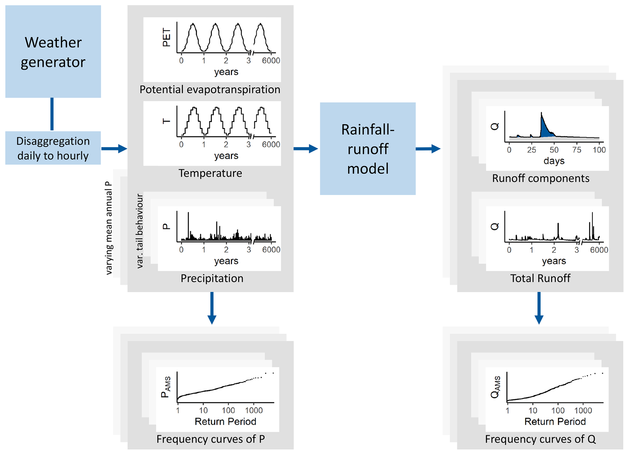
Figure 1 Sketch of the simulation model chain. Using a weather generator, time series of precipitation, temperature, and potential evapotranspiration are generated, which then feed into a conceptual rainfall–runoff model. From the simulated precipitation and discharge time series, annual maximum series are derived and their tail behaviour quantified.

2 Methods

Using a stochastic weather generator and a conceptual, spatially lumped rainfall–runoff model, we generate discharge times series (Fig. 1). This is followed by frequency analyses of the simulated precipitation and discharge time series and an analysis of the respective upper-tail behaviour. Different model set-ups are designed to address the research questions. To this end, the model is run on a synthetic catchment so that all model parameters can be varied freely within plausible ranges to values that are found to be most valuable for the analyses.

2.1 Simulation model chain

The first part of the simulation model chain is a stochastic multi-site, multi-variate weather generator which is set up based on observational data from stations in Germany (Hundecha et al., 2009; Nguyen et al., 2021). It is used to generate time series of precipitation P, temperature T, and potential evapotranspiration PET as input for the rainfall–runoff model. The weather generator has been evaluated to capture both the daily mean and the extreme (99.9th percentile) precipitation intensities well for a large set of weather stations in central Europe (Nguyen et al., 2021). The generated time series are based on observational data from the weather station in Bamberg (DWD, 2022). It is one of the stations with the longest available records of both daily and hourly data in Germany. For each configuration of the weather generator, 100 realizations of 60 years are generated with a daily resolution. Ten different configurations of the weather generator are produced to generate P time series with different tail behaviours. An extended generalized Pareto (extGP) distribution is fitted to the observed P data. While the scale and the lower shape parameter remain as fitted, the upper shape parameter of the extGP distribution is varied systematically by multiplying it by a factor between 0.2 and 2.0. This way, the upper shape parameter covers the range of values that was found when fitting extGP distributions to observations from the large set of central European weather stations analysed by Nguyen et al. (2021). Through this manipulation of the extGP upper-tail shape parameter, time series with different degrees of extreme frequency are created, despite using observations from just one station as initial input.

As the rainfall–runoff model is run on a small catchment, the temporal resolution of the input data needs to be higher than daily. A non-parametric method-of-fragments (MOF)-based method is applied to disaggregate the daily weather variables into hourly scale (Sharma and Srikanthan, 2006). The MOF is a commonly used method for the disaggregation of rainfall (e.g. Carreau et al., 2019; Li et al., 2018; Lu et al., 2015; Westra et al., 2012) and has been found to outperform other disaggregation models, especially for extreme rainfall characteristics (Pui et al., 2012). The MOF algorithm redistributes the daily value by borrowing hourly fragments from historical at-site records based on the k-nearest neighbour method. The seasonality-conditioned MOF, as described by Guan et al. (2023), is used to disaggregate P and T. As hourly PET records are not available, the fragments for PET daily-to-hourly disaggregation are assigned as 0.9 for day times (12 h, from 06:00 to 17:00) and 0.1 for night times (from 18:00 to 05:00).

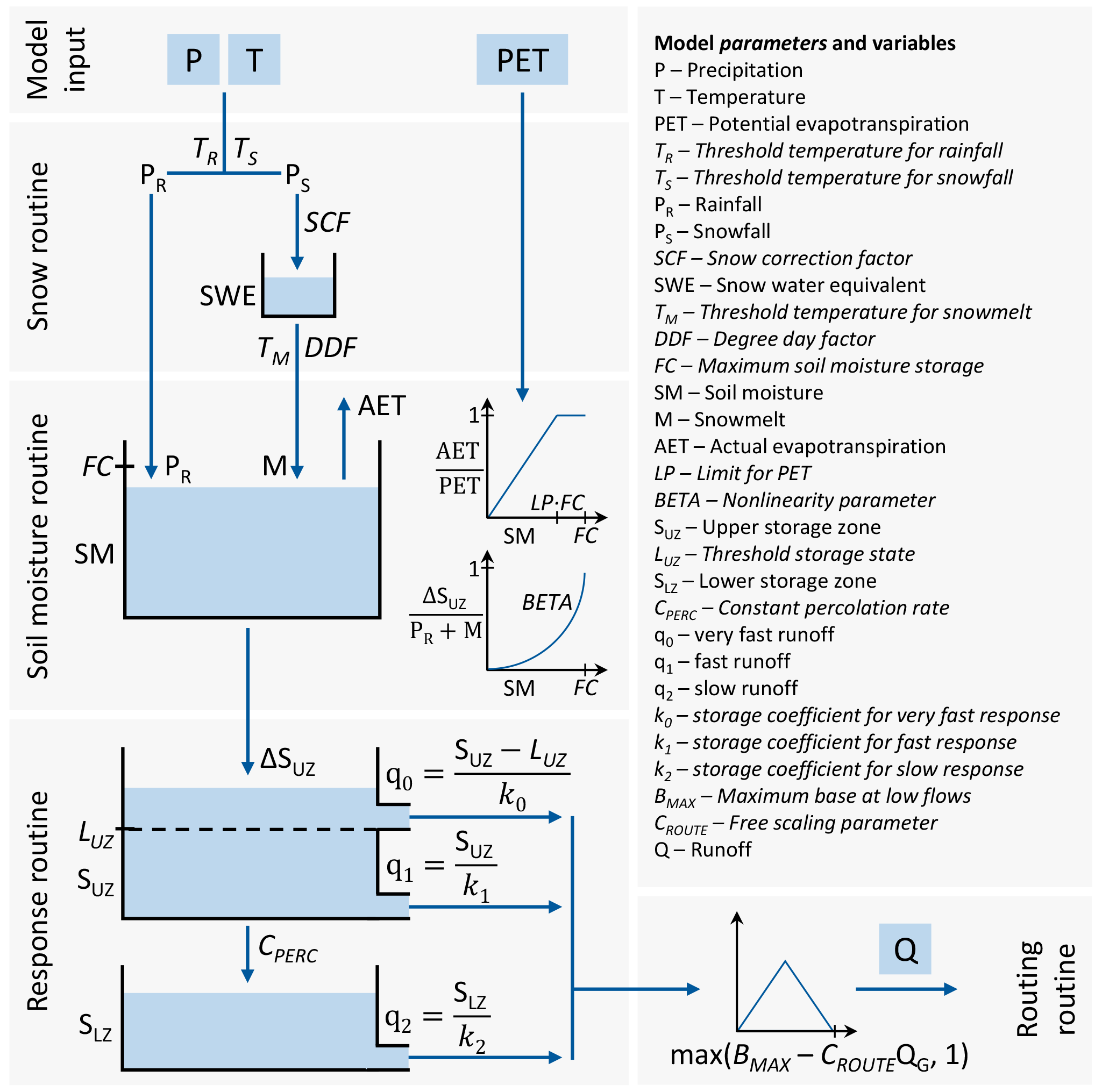
Figure 2 Schematic structure of the rainfall–runoff model TUWmodel (Parajka et al., 2007), which is a spatially lumped conceptual model following the structure of HBV.

The second part of the simulation model chain is a lumped conceptual rainfall–runoff model following the structure of the HBV model (R package TUWmodel; Parajka et al., 2007). It consists of a snow, a soil moisture, a response, and a routing routine with a total of 15 model parameters (Fig. 2). The model is run in a lumped way on a single synthetic catchment. Given the size of the catchment of 50 km², we assume homogeneous conditions throughout the catchment and a catchment response time at an hourly scale. This way, sub-catchment and routing processes should not affect the results.

The rainfall–runoff model is forced by the disaggregated output of the weather generator. The time series of T and PET are averaged to 1 year of data with diurnal and seasonal patterns, which is then repeated 6000 times (mean annual T = 9 ^∘C, annual PET sum = 817.8 mm). This minimizes confounding effects of T and PET on the discharge generation between different years and model runs. To characterize the tail heaviness of P, we fit GEV distributions to the annual maxima of hourly P series. All P series of 60 years with GEV shape parameters greater than 0.37 are excluded. These are GEV shape parameters well outside the observed range in Germany, where a maximum of 0.33 was estimated for time series of at least 75 years of daily precipitation (Vorogushyn et al., 2023). This way, 300 time series are excluded and the remaining 700 series of 60 years are grouped based on their shape parameters and combined into seven 6000-year-long time series. Using a slightly different cut-off than 0.37 for excluding P time series with very high GEV, shape parameters were not found to affect the findings. The remaining P time series are shifted to three different levels to represent dry, medium, and wet conditions that are typical in Germany. For this, the time series are multiplied with a factor of 0.9, 1.25, and 1.6 to have a mean annual P of 565, 784, and 1004 mm, respectively. The first year of each time series is used as a warm-up period for the model.

For addressing the effect of nonlinearity in the runoff generation, we focus on the exceedance of the storage capacity of an upper subsurface storage L_UZ as a threshold process. Its exceedance triggers an additional and faster runoff component q₀ (see Fig. 2). The model parameters most relevant for the exceedance of this storage capacity are found through a hybrid local–global sensitivity analysis which evaluates local sensitivity at several places throughout the parameter space (Melsen and Guse, 2021; Rakovec et al., 2014). Three parameters which physically cannot affect the storage exceedance are excluded from the sensitivity analysis (k₂, B_MAX, C_ROUTE; see Fig. 2). The remaining 12 parameters are varied between a low and a high value each, and with these parameter combinations the model is run for 3 years with the same P series as input for all runs. The parameters which are found to be least relevant as they each explain less than 3 % of the variation in the storage exceedance are subsequently fixed. In a second iteration, the remaining six parameters are varied between five values each. The aim of the second iteration is to evaluate which parameters are most relevant when the majority of parameters are already fixed to their final values. The parameters which combined explain at least 80 % of the variation in the exceedance of the storage capacity are taken as the relevant ones. These are then varied across their respective reasonable ranges for different model runs. Reasonable ranges are based on Parajka et al. (2007) with an adaption from the daily to the hourly timescale for all time-dependent parameters (i.e. DDF, k₀, k₁, k₂, C_PERC, B_MAX, and C_ROUTE). The same parameter ranges have been used by Ceola et al. (2015) for calibrating the TUWmodel for European catchments with different topographic and meteorological conditions and are therefore deemed appropriate for capturing many different extreme flood responses. The remaining parameters are kept fixed in all model runs. They are set based on values from Merz et al. (2011), who reported average parameter values based on model calibrations for 273 Austrian catchments. Again, time-dependent parameters have to be adapted from the daily to the hourly scale. All parameter values and ranges are listed in Table A1.

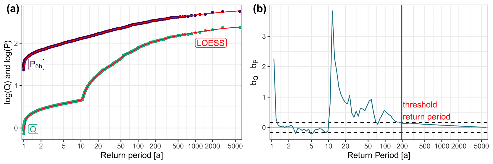
Figure 3 (a) Frequency curves of flood peaks (Q) and 6 h precipitation maxima (P_6 h) on a log–log plot for one exemplary simulation run. Locally estimated scatterplot smoothing (LOESS) is applied, and the slope between each pair of points is estimated. (b) Difference between the slopes b of P_6 h and Q. When the curves run in parallel, the difference between the slopes tends to zero. The dashed black lines indicate a buffer around zero within which the difference between slopes needs to lie to assume that the flood peak distribution is governed entirely by the rainfall distribution. The return period beyond which this is the case is referred to as threshold return period.

For each model run, the output consists of the simulated discharge time series Q along with the time series of the very fast runoff component q₀ and the respective model parameters and precipitation time series which were used in the model run.

2.2 Analysis of the simulated time series

For all time series of P and Q the annual maxima are derived. For P this is done for different durations, namely 1, 2, 3, 6, and 12 h. For each annual maximum of Q, it is derived whether the very fast runoff component q₀ contributed to the peak, i.e. whether or not the storage capacity L_UZ was exceeded (see Fig. 2). GEV distributions are fitted to the annual maximum series (AMS) of P and Q using L moments. Different time series lengths (60 to 6000 years) are used for fitting GEV distributions to see how this affects the tail behaviour and its controls. It should be noted that the shape parameter of a GEV distribution fitted to a time series of limited length does not necessarily reflect the true tail behaviour of the underlying distribution but is only an approximation thereof. When fitting GEV distributions to subsets of a time series of different lengths, the shape parameters may vary due to differences in the estimation uncertainties. To reflect this, we will use the terminology “apparent tail behaviour” when drawing conclusions based on the GEV shape parameter of a distribution fitted to a limited time series.

To examine threshold return periods beyond which the flood peak distribution is governed entirely by the rainfall distribution, the two distributions are evaluated on log–log plots. On such a plot, it is assumed that beyond the threshold return period the slope of the distribution of Q is the same as the slope of the distribution of P, given that P is considered “over a duration of the order of the time of concentration” (Gaume, 2006) of the catchment. To evaluate the identity of slopes on a log–log plot, local slopes of the logarithmic values of the annual maxima of Q and P against their return periods are estimated. For this, locally estimated scatterplot smoothing (LOESS) is first applied to the annual maxima (see an example in Fig. 3), as otherwise even small irregularities in the curves could strongly affect the threshold return period. Based on the smoothed curves, slopes are estimated for neighbouring pairs of points.

To check which duration of P is best in line with the concentration time of the catchment, the differences between slopes of P and Q are estimated for model runs for “impervious” catchments and for different durations of P, namely 1, 2, 3, 6, and 12 h. The catchment in a model run is considered to be close to impervious when the maximum soil moisture storage FC, the limit of the upper subsurface storage L_UZ, and the percolation rate to the lower subsurface storage C_PERC are set to values close to zero (FC = L_UZ = 1 mm and C_PERC = 0.00042 mm h⁻¹). The duration of P for which the sum of differences between the slopes of P and Q is lowest best represents the concentration time of the catchment and is used for the subsequent analyses (denoted P_ct). One might expect that for impervious catchments, the curves of Q and P_ct do not only run in parallel but are identical. This is not the case for our model set-up for the following reason: in the TUWmodel, evapotranspiration is active even during extreme rainfall events, and so Q is always lower than P_ct by at least the amount of actual evapotranspiration taking place. This is a shortcoming of the model, but it does not affect our findings as for our analyses only the slopes of the curves and not their distance to each other are relevant.

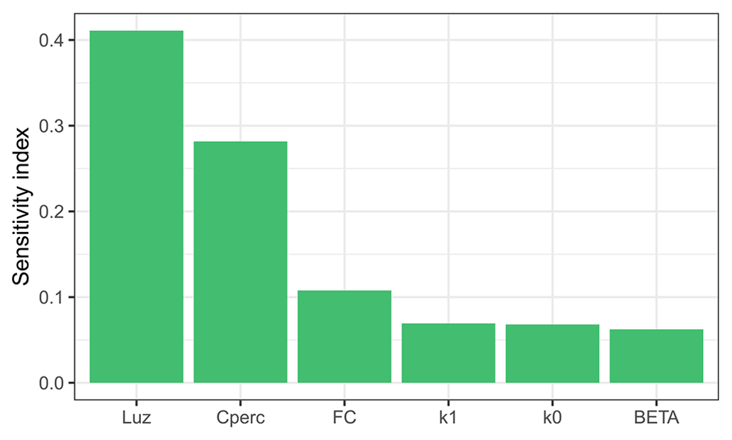
Figure 4 Relevance of six model parameters for the exceedance of the storage capacity L_UZ as derived through a hybrid local–global sensitivity analysis. The sensitivity index describes which share of the total variation in the exceedance of L_UZ observed in all model runs of the sensitivity analysis can be attributed to changes of one specific model parameter.

In theory, the difference between the slopes of curves which run in parallel is zero. However, the differences between the slopes of P and Q are hardly ever exactly zero, even though they are based on smoothed curves. Therefore, a buffer around zero is defined based on the differences between the slopes of P_ct and Q estimated for model runs on close to impervious catchments (i.e. FC = L_UZ = 1 mm and C_PERC = 0.00042 mm h⁻¹). For close to impervious catchments, the curves of P_ct and Q are assumed to run in parallel for all return periods. The 99th percentile of the differences estimated for return periods of 2 years and greater is taken as the buffer within which slope differences need to lie for the curves to be considered parallel. To evaluate the sensitivity of the threshold return period to the definition of the buffer, also the 95th percentile and the maximum are briefly considered.

Finally, the return period from which onward the difference between the slopes of P_ct and Q is within the buffer is considered the threshold return period beyond which the flood peak distribution is governed entirely by the rainfall distribution (Fig. 3). The estimated threshold return periods are compared to catchment characteristics, i.e. to the model parameters which are varied between model runs and to mean annual precipitation levels.

To analyse whether nonlinear runoff generation leads to heavy-tailed flood peak distributions, the AMS of Q are classified into two groups based on whether or not there is a process shift in the AMS. A process shift means here that for some but not all of the flood peak events the storage capacity L_UZ was exceeded, and the very fast runoff component q₀ was active. This is analysed for AMS of Q of different lengths, namely 60, 200, 1000, and 6000 years. This way we can compare results for very long time series and time series of typically observed lengths. Finally, the relation of the tail behaviour of P and Q is assessed for the two groups and the four different time series lengths.

3 Results

Using a hybrid local–global sensitivity analysis, the model parameters most relevant for the exceedance of the storage capacity L_UZ (see Fig. 2) were identified. The three most relevant parameters are the upper subsurface storage capacity itself (L_UZ), the maximum soil moisture storage (FC), and the percolation rate from the upper to the lower subsurface storage (C_PERC) (Fig. 4). It is not surprising that the value of the storage capacity itself is most relevant for how frequently it is exceeded. FC affects how much water enters the subsurface storage, while C_PERC is one of the parameters affecting the outflow from the subsurface storage (Fig. 2). In this way, they both have an influence on the amount of water stored in the upper subsurface storage in each time step and with that also on whether or not the storage capacity is exceeded.

It is commonly assumed (e.g. in the rational method) that rainfall over the duration of the time of concentration of a catchment results in the largest flood peaks (Michailidi et al., 2018). To analyse whether the rainfall distribution dominates the flood peak distribution beyond a threshold return period, the precipitation should be examined over this specific duration. To find the appropriate duration, the differences between slopes of P and Q were estimated for model runs on close to impervious catchments (FC = L_UZ = 1 mm and C_PERC = 0.00042 mm h⁻¹) for durations of P of 1, 2, 3, 6, and 12 h. The lowest sum of differences between the slopes – and with that the closest link between rainfall and flood peaks – was found for a duration of 6 h (Fig. B1). A time of concentration of 6 h is considered realistic for a catchment of 50 km². Different formulas for estimating the time of concentration based on various catchment characteristics result in values of, for example, 2 h (Haktanir and Sezen, 1990) or 12 h (Ganguli and Merz, 2019). All subsequent analyses are based on P over this duration (P_6 h).

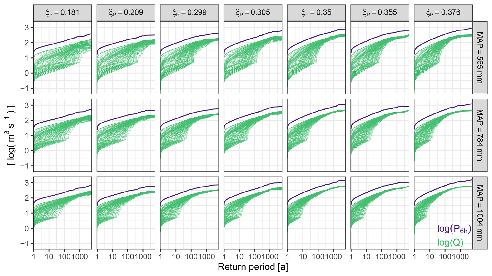
Figure 5 Logarithmic values of the annual maxima of 6-hourly rainfall P_6 h and discharge Q against their return periods. Time series of Q were simulated with a rainfall–runoff model which uses the P series as input. Different subplots vary in the mean annual precipitation (MAP) level and the tail behaviour (characterized with the GEV shape parameter ξ) of P. Differences in the curves of Q within each subplot are related to different parameterizations of the rainfall–runoff model.

The curves of all P_6 h series along with the respective simulated Q series are displayed on log–log plots in Fig. 5. The shapes of the Q distributions simulated with one and the same P distribution show a large variability. Some AMS of Q show distinct step changes similar to the one visualized in Fig. 3a, while others seem to run in parallel to P_6 h across all return periods. For most model set-ups, Q appears to run in parallel to P_6 h eventually. This is analysed quantitatively further down. Figure 5 also demonstrates that P_6 h and Q are not superimposed for any of the set-ups. As stated in Sect. 2.2, the distance between the curves of P_6 h and Q is related to the actual evapotranspiration which can occur even during extreme rainfall events in the TUWmodel.

The threshold return period (RP) beyond which the frequency curves of P_6 h and Q run in parallel varies between model runs, i.e. between catchments with different characteristics (Fig. 6). The characteristics considered here are both precipitation characteristics and runoff generation characteristics. In some catchments, the threshold RP is around 2 years – in these catchments, the maximum soil moisture FC and the threshold of the upper subsurface storage L_UZ were set to 1 mm each. These catchments are basically impervious, and even small floods are governed entirely by precipitation. For the highest number of catchments, the threshold RP is between 100 and 500 years. In these catchments, the rainfall distribution governs the flood peak distribution beyond a RP of 100 to 500 years.

When grouping the results based on the mean annual precipitation (MAP) level of the P time series used as model input, we see a shift to lower threshold return periods with increasing MAP (Fig. 6). MAP should be interpreted here as a measure of overall catchment wetness which controls the mean event rainfall depth. For the two highest MAP levels, the largest share of catchments exhibits a threshold RP around 150 years. For the highest MAP of 1004 mm there is also a substantial share of catchments with threshold RPs below this, while for the medium high MAP of 784 mm many catchments exhibit threshold RPs beyond 200 years. For the lowest level of MAP, the highest density of threshold RPs is found around 450 years.

For some catchments, no threshold RP was found within 6000 years of annual maxima. In these cases, either no threshold RP exists or the threshold RP is beyond 6000 years. The first alternative would mean that the rainfall distribution never governs the flood peak distribution entirely, which is deemed unlikely based on the literature presented in Sect. 1 and also from physical considerations: for all catchments a point is reached eventually where rainfall is so extreme that saturation occurs and rainfall translates directly to runoff. The number of catchments with no threshold RP within 6000 years varies between the different levels of MAP. While no threshold RP within the considered time series was found in 22 % of the model runs with a MAP of 565 mm, this was only the case for 2 % of models runs with a MAP of 1004 mm.

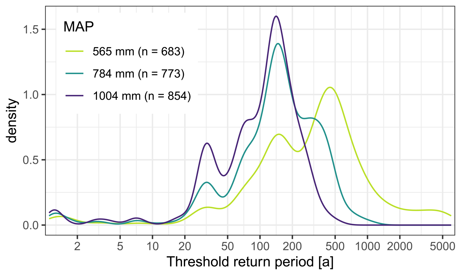
Figure 6 Density plot of the threshold return periods derived in 875 model runs per mean annual precipitation (MAP) level. The number in brackets indicates for how many model runs a threshold RP was found within 6000 years. The threshold return period describes beyond which return period the frequency curves of discharge and precipitation run in parallel on a log–log plot, i.e. beyond which return period the flood peak distribution is governed by the rainfall distribution. For some catchments no threshold RP was found within 6000 years of annual maxima.

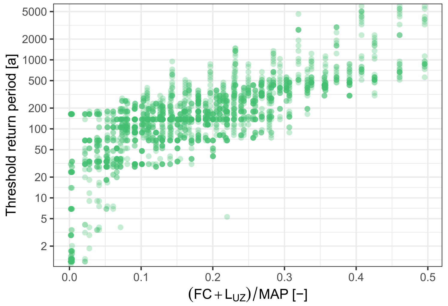
Figure 7 The relation of threshold return periods and the ratios of catchment storages to the mean annual precipitation (MAP). Catchment storages are characterized by the sum of the maximum soil moisture storage FC and the limit of the upper subsurface storage L_UZ. Results are based on 2310 model runs in which a threshold return period within 6000 years was estimated. The threshold return period describes beyond which return period the frequency curves of discharge and precipitation run in parallel on a log–log plot, i.e. beyond which return period the flood peak distribution is governed by the rainfall distribution. Different shades of green arise through different densities of points.

To see if the threshold return period is related to catchment characteristics, it was analysed against the three model parameters that were varied between model runs. The percolation rate to the lower groundwater storage (C_PERC) does not show an influence on the threshold RP (Fig. B2). The other two characteristics, i.e. the maximum soil moisture storage (FC) and the limit of the upper subsurface storage (L_UZ), both quantify water storages in the catchment. The ratio of the combined storages to the MAP is related to the threshold RP: larger ratios of storage to MAP tend to lead to larger threshold RPs (Fig. 7). Threshold RPs below 30 years are only estimated for catchments where the combined volume of the storages is less than 7.1 % of the MAP, with one single exception. In contrast, high threshold RPs beyond 1500 years are only estimated for catchments with storage–MAP ratios greater than 30 %.

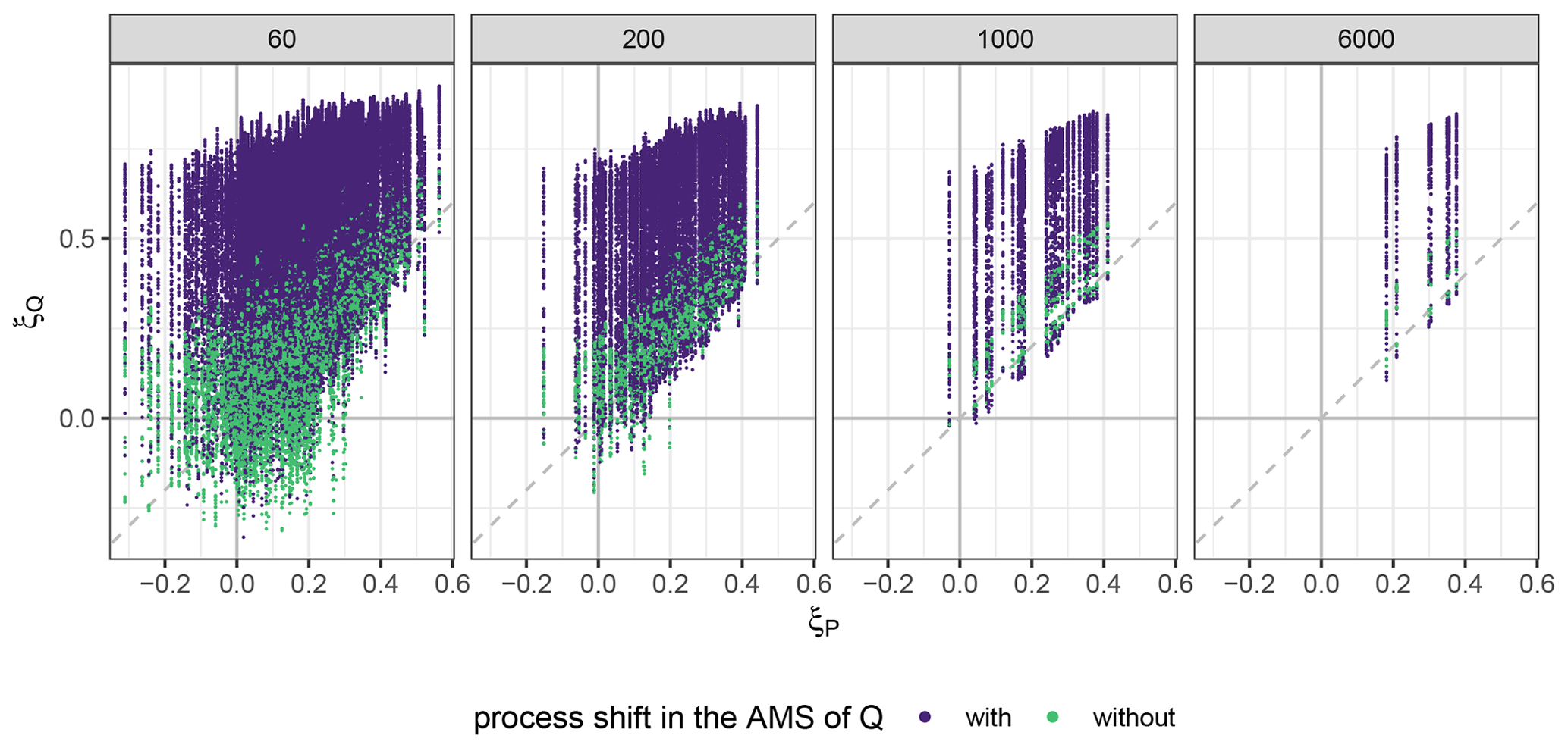
Figure 8 Shape parameters of generalized extreme value (GEV) distributions fitted to discharge series (ξ_Q) against GEV shape parameters of the precipitation series (ξ_P) that were used to simulate the discharge. Q is considered on an hourly scale, while P is considered on a 6-hourly scale. GEV distributions were fitted to annual maximum series (AMS) of 60, 200, 1000, and 6000 years. Results are based on 875 model runs of 6000 years – 7 P series with different tail behaviour but same MAP and 5³ different parameter sets in the rainfall–runoff model. An AMS of Q was classified as containing a process shift when for some but not all of the flood peak events a storage threshold was exceeded and an additional and faster runoff component was triggered.

The estimation of the threshold RP is based on the somewhat arbitrary definition of the buffer around zero within which slope differences need to lie to classify curves as parallel. To evaluate different buffer choices and their effect on the resulting threshold RPs, we considered the 95th, 99th, and 100th percentile of the slope differences estimated for close-to-impervious model runs as buffer values. As expected, a wider buffer around zero results in overall smaller threshold RPs. Similarly, the number of catchments without threshold RP within 6000 years increases as the buffer around zero gets narrower. Plots such as the ones in Figs. 6 and 7 were considered for all three buffer levels along with visual inspections of selected model runs (not shown). When using the 95th percentile, many model runs with close-to-impervious conditions showed threshold RPs beyond 5 or even 10 years. This is not in line with the assumption that for impervious catchments the frequency curves of P_6 h and Q should run in parallel for all return periods. On the other hand, using the 100th percentile led to many very low threshold RPs for curves of P_6 h and Q which would not be considered parallel in a visual inspection. Therefore, the 99th percentile is considered the most appropriate.

GEV distributions are fitted to AMS of different lengths of Q and P_6 h and their shape parameters compared. In the following, only the results based on model runs with the medium level of MAP, i.e. 784 mm, are presented. The results for low and high MAP are qualitatively similar and can be found in Fig. B3. For the entire time series length, i.e. 6000 years, the estimated GEV shape parameters of P_6 h vary between 0.18 and 0.38 (Fig. 8). The estimated GEV shape parameters of flood peak distributions vary between 0.11 and 0.85 for 6000-year-long series. Hence, one rainfall distribution can result in very different flood peak distributions – even for time series of 6000 years.

The annual maxima of Q are classified into two groups based on whether or not there is a process shift in the AMS. An AMS is considered to have a process shift when for some but not all of the flood peak events the capacity of the upper subsurface storage was exceeded and the very fast runoff component of the model was active. When comparing shape parameters of Q against those of P_6 h for 6000-year-long series, the estimated shape parameters of model runs where no process shift occurred in the runoff generation scatter closer around the 1:1 line than the ones with process shift. That means that without a process shift, a higher shape parameter of P_6 h tends to lead to a higher shape parameter of Q (Fig. 8). In contrast, the range of estimated shape parameters of Q in model runs with a process shift is much larger. Overall much higher values are found in these cases, which means that flood peak series with a process shift in the runoff generation tend to have stronger apparent heavy-tail behaviour than those without a process shift.

For time series of shorter length, the ranges of estimated GEV shape parameters are larger than for 6000-year-long series. This is expected due to the larger estimation uncertainties for shorter time series. For 60-year-long subsets of P, the estimated GEV shape parameters vary between −0.31 and 0.56 (Fig. 8). As described in Sect. 2.1, P series with a shape parameter greater than 0.37 were originally excluded. However, this was done for the hourly P data, while the results presented here are based on 6-hourly P. The estimated GEV shape parameters of flood peak distributions vary between −0.33 and 0.92 for 60-year-long subsets. As for the 6000-year-long series, one rainfall distribution can result in very different flood peak distributions, and the range of estimated shape parameters of Q per shape parameter of P gets even higher for shorter time series. With regards to the occurrence of a process shift, similar results are observed for the short subsets as for the long time series: higher GEV shape parameters are estimated for the cases where a process shift occurred as opposed to the ones without process shift in the AMS.

4 Discussion

Threshold return periods beyond which the rainfall distribution dominates the flood peak distribution were found to vary depending on catchment characteristics. In many cases the threshold RP is 100 years or larger. This estimate lies between the GRADEX method and findings from Gaume (2006). Gaume (2006) suggested to consider the “distribution of the maximum mean rainfall intensity over a duration of the order of the time of concentration of a watershed” for estimating floods with return periods beyond 500 years. In contrast, in the GRADEX approach, the rainfall distribution is assumed to govern the flood peak distribution beyond return periods of 10–20 years for impermeable and beyond 50 years for more permeable catchments (Naghettini et al., 2012). While for a few cases with small water storages we did find threshold RPs below 20 years, we estimated larger threshold RPs for the majority of cases. A similar range of threshold RPs was found by Brunner et al. (2021) in relating future changes in precipitation magnitudes with future changes of flood magnitudes for 78 catchments. They found that, above a certain threshold RP, future increases in rainfall translate to increased flood magnitudes, while for smaller events this is not the case. The threshold RPs that they estimated range between 10 and 200 years.

In some catchments, the rainfall distribution and flood peak distribution do not run in parallel at all within 6000 years. This means that either the threshold RP is beyond 6000 years or it does not exist. The latter is deemed unlikely based on the reviewed literature (e.g. Gaume, 2006; Merz et al., 2022) and hydrological process understanding. Every catchment should be saturated eventually if the precipitation is extreme enough, and the corresponding part of the flood peak distribution should then be governed entirely by the rainfall distribution. For some catchments, the return period of such saturating rainfall events might be extremely large. In addition, the share of catchments where no threshold RP was detected within 6000 years decreases with increasing MAP, i.e. with increasing overall catchment wetness. This suggests that, for very high MAP, all catchments would have a threshold RP within 6000 years. It also clearly supports the assumption that not detecting a threshold RP within 6000 years simply means that it occurs at an even larger RP.

Larger ratios of catchment storage to MAP are found to lead to higher threshold RPs. This is explained as follows: the smaller the storage, the more frequent it fills up and saturation excess runoff is triggered. This means that already for small rainfall events, i.e. with a low RP, saturation can be reached and therefore rainfall also starts to dominate the flood peak distribution for lower RPs. Similarly, Rogger et al. (2013) found that the RP of a step change in the flood frequency curve increases with increasing storage deficit in a catchment. The relation depicted in Fig. 7 allows the estimation of threshold RPs without the use of streamflow observations, simply by estimating the ratio of catchment storages to MAP. This assumes that the found relation between storage–MAP ratio and threshold RP can be transferred to the real world, which would still need to be verified. To test this, comparisons with real-world observations and further studies using, for example, other hydrological models would be required.

The percolation rate to the lower subsurface storage does not show an effect on the threshold RP. While it does affect the water level in the upper subsurface storage, it seems to do so on a longer timescale than is relevant for the generation of very fast runoff during heavy-rainfall events. In their study on future changes, Brunner et al. (2021) found that the threshold RP beyond which increases in precipitation translate to increases in flood magnitude is modulated by elevation, season, and event type. While we did not analyse those characteristics here, similar influences can be expected for the link between rainfall and flood peak distributions studied here as for the link between future changes. For example, Brunner et al. (2021) found a much lower threshold RP in high-elevation catchments compared to low-elevation catchments. This aligns with our finding of lower threshold RPs for lower catchment storages, assuming that high-elevation catchments usually exert lower subsurface storage capacities.

We found that the same rainfall distribution can result in flood peak distributions with very different apparent tail behaviour. This is in line with the findings from McCuen and Smith (2008) and Gottschalk and Weingartner (1998). It might seem counter-intuitive that even for 6000-year-long time series the GEV shape parameter of the flood peak distribution can vary strongly from the shape parameter of the rainfall distribution, even though we found that the frequency curves of P and Q run in parallel within 6000 years for most catchments. However, even when the tail of the rainfall distribution controls the tail of the flood peak distribution asymptotically, both distributions do not necessarily have the same shape parameter when estimated for a time series of limited length. In this case, the shape parameter quantifies the apparent tail behaviour of the distribution, and fitting the distribution takes all annual maxima into account. This means that also the smaller annual maxima – where frequencies of P and Q usually still vary – have an effect on the estimated GEV shape parameter.

Analysing time series of different lengths indicates the effect that sampling uncertainty has and helps relate the findings to the estimation of the apparent tail behaviour of observed time series of limited length. For all time series lengths, higher shape parameters of rainfall distributions tend to lead to higher shape parameters of flood peak distributions, but the variability is large. However, for time series longer than 200 years and shape parameters of P greater than 0.2, the shape parameter of P seems to be a kind of lower bound for the estimated shape parameter of Q (Fig. 8). A heavy-tailed rainfall distribution does not lead to a light-tailed flood peak distribution. This is different for time series of 60 years: a rainfall distribution with an estimated shape parameter of around 0.2 can also result in a flood peak distribution with an estimated shape parameter well below zero. This is due to the higher sampling uncertainty for short time series as we do not see this for the longer series. For long series of P with a heavy-tailed distribution, it is more likely that some extreme discharge events are generated which can make the tail of the flood peak distribution heavy. For shorter time series, such events are not always included in the series. When fitting a GEV distribution to observed flood peaks, it could therefore be useful to use the estimated shape parameter of the rainfall distribution as a lower bound for the shape parameter of the flood peak distribution – especially when the observed record of precipitation is longer than that of streamflow.

Some of the estimated shape parameters of flood peak distributions are higher than what has been previously estimated for observed data in Germany. At 480 gauges in Germany and Austria, the maximum shape parameter estimated for observed streamflow records of at least 60 years length is 0.471 (Macdonald et al., 2022). There are several reasons why we find even heavier tails in the simulated streamflow series. Firstly, not all model runs necessarily represent realistic central European catchment conditions. While each model parameter individually was varied over a plausible range, we considered all combinations of the parameter values without checking if the combinations are reasonable as well. For example, some combinations result in flood frequency curves with very sharp and large step changes, similar to the one depicted in Fig. 3. In addition, we use some P time series as input for which the distribution shows heavier tails than for observed P time series. As mentioned before, the maximum shape parameter for observed rainfall distributions in Germany is 0.33 (Vorogushyn et al., 2023) and we use values up to 0.37. Papalexiou and Koutsoyiannis (2013) argue based on 15 000 precipitation records worldwide that when correcting for the record length the “true” shape parameter is even expected to be in the range between 0 and 0.23 with 99 % confidence. Since we want to see the whole spectrum of what could potentially be possible, we decided against further narrowing the range of shape parameters of rainfall distributions used as input, against limiting the parameter combinations, and against filtering out frequency curves that look different to what has been observed so far.

When there is no process shift in the runoff generation, the estimated shape parameter of Q is more closely related to the estimated shape parameter of P compared to cases with a process shift. In the cases with a process shift in the runoff generation, the estimated shape parameter of Q can be lower than the estimated shape parameter of P – especially for short time series length – but for the majority of model runs it is much higher. In general, much higher shape parameters of Q are found when a threshold process is present in the runoff generation; i.e. this nonlinear behaviour of the runoff generation leads to flood peak distributions with apparent heavy-tail behaviour. Several studies have linked threshold processes in the runoff generation to step changes in flood frequency curves (e.g. Kusumastuti et al., 2007; Struthers and Sivapalan, 2007; Rogger et al., 2012), but now we showed that they also lead to flood peak distributions with higher estimated GEV shape parameters and apparent heavy-tail behaviour.

In this study, we fit one GEV distribution to the data even when we know that there is a process shift in the runoff generation. This might actually violate the assumption of independent and identically distributed (IID) values for distribution fitting, if the values below and above the threshold are not identically distributed. Having values from two different sub-distributions, i.e. below and above the threshold, would require a mixture distribution (e.g. Fischer, 2018). If we still fit one GEV distribution to the entire data, it does not represent the true underlying distribution and also not the true tail behaviour. However, in practice and for observed values we usually do not know if the values are from different sub-distributions and therefore simply fit one GEV distribution to the entire observed data. We did the same here to make the results more relatable and applicable to observed time series. Our results indicate though that this common practice can be problematic at times because a GEV distribution is not always a good fit, even when considering annual maxima. While the GEV distribution is the asymptotic distribution of independent block maxima (Fisher and Tippett, 1928), we usually consider time series of limited length and pre-asymptotic behaviour. A detailed discussion about such differences between the statistical and hydrological perspective on GEV distributions and their tail behaviour can be found in Merz et al. (2022).

For return periods mainly relevant to flood risk management, i.e. 30–200 years, runoff generation is a more pronounced control of flood peak tail behaviour than precipitation – at least for small homogeneous catchments in central Europe. Assuming that the rainfall distribution can be used to extrapolate the flood peak distribution from a return period of 20 or 50 years onwards, as for example in the GRADEX method (Naghettini et al., 2012), which should only be done with care – threshold processes in the runoff generation can strongly affect frequency curves. Approaches like the GRADEX method should only be used for high RPs or if it can be ruled out that process shifts in the catchment response might occur for larger events. If within a short, observed time series there are any indications that different processes act for the largest events than for the smaller ones, it makes sense to assume a heavy-tailed distribution even if the fit to the data is not heavy-tailed. Such indications could be for example when distinctively higher runoff coefficients or shorter event timescales are estimated for the largest observed events compared to smaller ones (Macdonald et al., 2022; Rogger et al., 2012).

The findings from this study are limited in the way that they do not include effects of spatial variability or different catchment sizes. Spatial variability in rainfall has been linked to heavy-tailed flood peak distributions, and it has been shown that this effect depends on the catchment size (Wang et al., 2023). Increasing spatial variability in soil moisture storage leads to a decrease in step changes in flood frequency curves as not all areas generate overland flow at the same time (Rogger et al., 2013). It is not clear if this would also affect the value of the threshold RP beyond which the rainfall distribution dominates the flood peak distribution. To address this, the simulations would have to be repeated with spatial variability of rainfall and runoff characteristics instead of using a spatially lumped model. Along with this, the catchment size could be increased and results evaluated for sub-basins of different spatial extent. However, in such a set-up, tail heaviness could be affected by a combination of catchment size, sub-basin response, spatial organization, and river routing characteristics, making it difficult to isolate the effects of precipitation and runoff generation. Based on this rationale, we decided for a simplified catchment representation without spatial variabilities. Expanding this set-up in future studies is however deemed very interesting and advisable.

Furthermore, our findings are based on synthetic catchments and simulation runs. While such an approach has major advantages like the generation of long time series, results are not always directly transferable to the real world. For example, in the adopted rainfall–runoff model only one nonlinearity in the runoff generation was considered, namely the activation of an additional very fast runoff component. However, in a real catchment multiple nonlinearities and process shifts might be present such as the onset of overland flow, the onset of subsurface stormflow, the activation of macropores, or the temporary expansion of the river network. The model does not include all these processes explicitly and is therefore, as all models, a simplified representation of reality. Hence, the simulated flood peak distributions are also only representative of this simplified reality. Nevertheless, they can help us explore results which can be valuable for real-world applications. In fact, Brunner et al. (2021) concluded that there is a “growing body of real-world evidence” suggesting that a precipitation-flood response threshold exists across a wide range of hydrologic and hydroclimatic regimes (e.g. Do et al., 2020; Wasko and Nathan, 2019; Bertola et al., 2020). This strongly supports the relevance of our findings for real-world catchments. In addition, the model components used have been shown to represent well real-world behaviour when calibrated with real-world data (e.g. Nguyen et al., 2021; Ceola et al., 2015; Parajka et al., 2007). Nevertheless, the simulation model chain and its parameterization has been set up for central European conditions, and so the findings should not be directly transferred to other regions of the world where conditions are very different.

5 Conclusions

Both runoff generation processes and rainfall characteristics are assumed to affect the tail behaviour of flood peak distributions. Rainfall distributions have been suggested to govern flood peak distributions beyond a certain return period. Here, we analysed where such a threshold return period lies and if this is linked to catchment characteristics. In addition, we were interested in processes that govern flood peak tail behaviour for return periods below this threshold return period. In particular, we analysed whether nonlinear runoff generation that is caused by threshold processes leads to heavy-tailed flood peak distributions. To address these questions, we used a simulation-based approach consisting of a weather generator and a rainfall–runoff model. Long time series of precipitation and streamflow were generated and their tail behaviour subsequently assessed.

We found that the threshold return period (RP) beyond which the rainfall tail dominates the flood peak distribution varies strongly between catchments. For the majority of the analysed synthetic catchments, the threshold RP lies between 100 and 500 years. Overall, threshold RPs from below 2 years to beyond 6000 years were estimated. We found that the threshold RP increases with an increasing ratio of catchment storage to mean annual precipitation (MAP). MAP reflects here the overall catchment wetness and controls the mean event rainfall depth. The larger the storage–MAP ratio in a catchment, the higher is the threshold RP beyond which the rainfall tail dominates the tail of the flood peak distribution.

When comparing the shape parameters of generalized extreme value (GEV) distributions fitted to precipitation and discharge, we found a much larger variability for the latter than for the former. Independent of the time series length, the same rainfall distribution can result in flood peak distributions that differ strongly in their tail behaviour. For time series of 200 years and more, the shape parameter of the rainfall distribution appeared like a lower bound for the shape parameters of the resulting flood peak distributions. When fitting a GEV distribution to observed flood peaks, it could therefore be useful to assume the shape parameter of the rainfall distribution as the lowest possible value for the shape parameter of the flood peak distribution. This can be especially useful when the observed record of precipitation is longer than that of streamflow, so that for the rainfall tail more robust estimations can be achieved than for the flood peak tail.

Threshold processes in the runoff generation were found to lead to flood peak distributions with stronger apparent heavy-tail behaviour. Catchments where a process shift in the runoff generation occurred had generally flood peak distributions with higher estimated GEV shape parameters than the ones without process shift. The process shift considered here is caused by a threshold in the upper subsurface storage. When this threshold is exceeded, an additional and faster runoff component is triggered. Distributions with such a process shift tend to show a step change. While the step change itself does not characterize the tail of the distribution, it does result in a higher estimated value of the shape parameter of the fitted GEV distribution. The finding suggests that if within a short, observed time series there are any indications that different processes act for the largest events than for the smaller ones, it might be useful to assume a heavy-tailed distribution even if the distribution originally fitted to the data is not heavy-tailed.

Overall, both rainfall and runoff generation were found to be important controls of the tail behaviour of flood peak distributions. The runoff generation can strongly modulate tail behaviour, especially through threshold processes. Beyond a certain return period, the influence of catchment processes decreases and the tail of the rainfall distribution starts to dominate the tail of the flood peak distribution. Beyond which return period this is the case depends on catchment characteristics, in particular on catchment storage in relation to mean annual rainfall amount. In many catchments, the runoff generation is found to be a more pronounced control of flood heavy tails than precipitation for return periods which are mainly of interest to flood risk management. However, these findings are based on small, spatially homogeneous catchments. Future studies should address the effect that spatial variability and catchment size have on flood peak tail behaviour and its relation to runoff generation and rainfall characteristics.

Appendix A: Model parameters

Table A1 Parameter values and ranges of the TUWmodel as they are used in the sensitivity analysis (SA) and in the final model runs (MRs). Ranges are based on Parajka et al. (2007); fixed values are based on Merz et al. (2011). A schematic of the model structure with the model parameters can be found in Fig. 2.

Appendix B: Additional figures

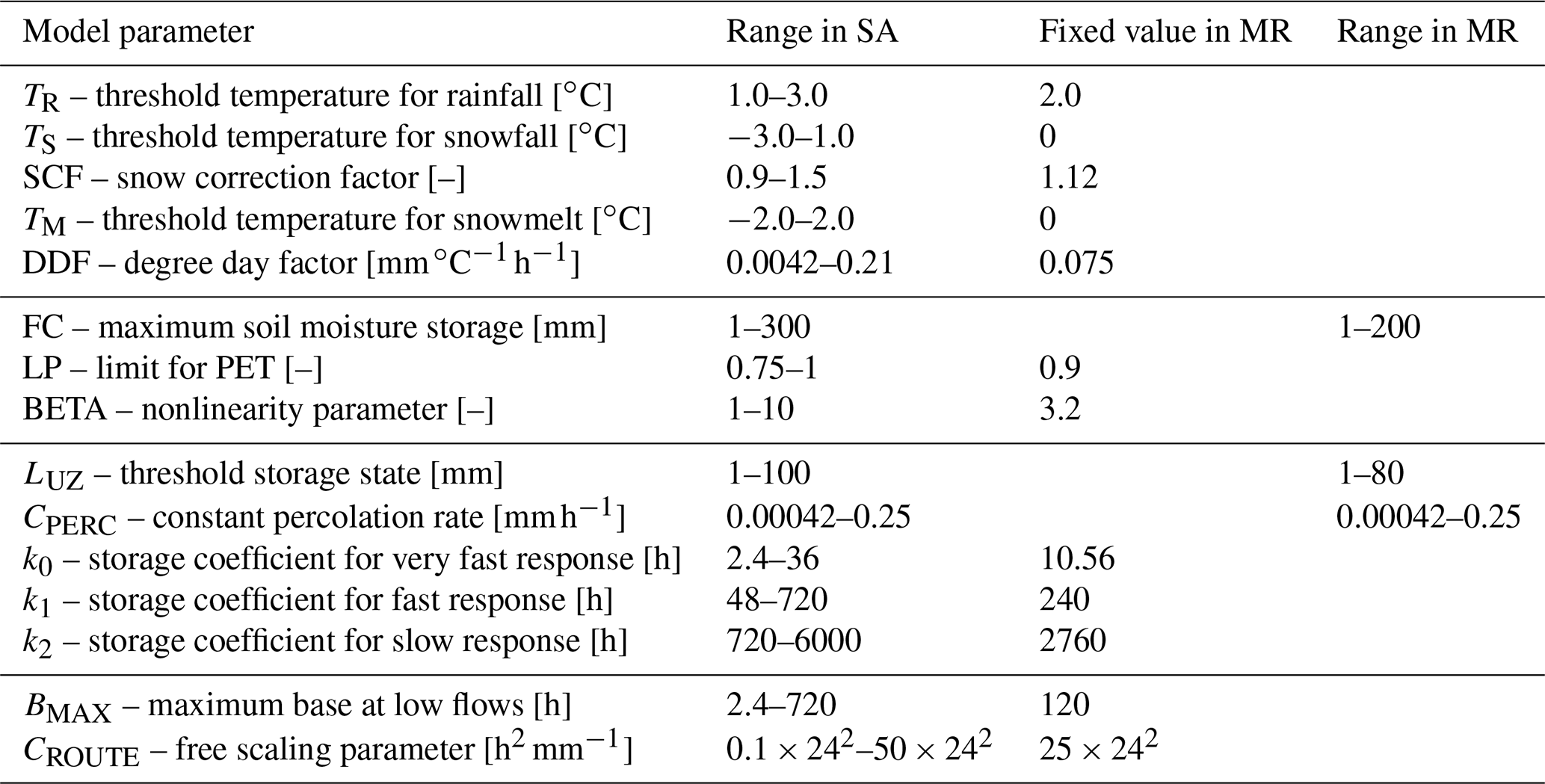
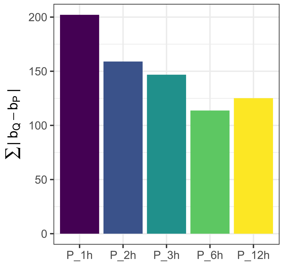
Figure B1 Sums of absolute differences between the slopes of discharge (Q) and precipitation (P) frequency curves for different durations of P. Local slopes of log (Q_AMS) and log (P_AMS) against their return period were estimated for 21 model runs on close-to-impervious catchments for each duration of P. The smaller the sum of absolute differences, the closer a duration of P is linked to Q.

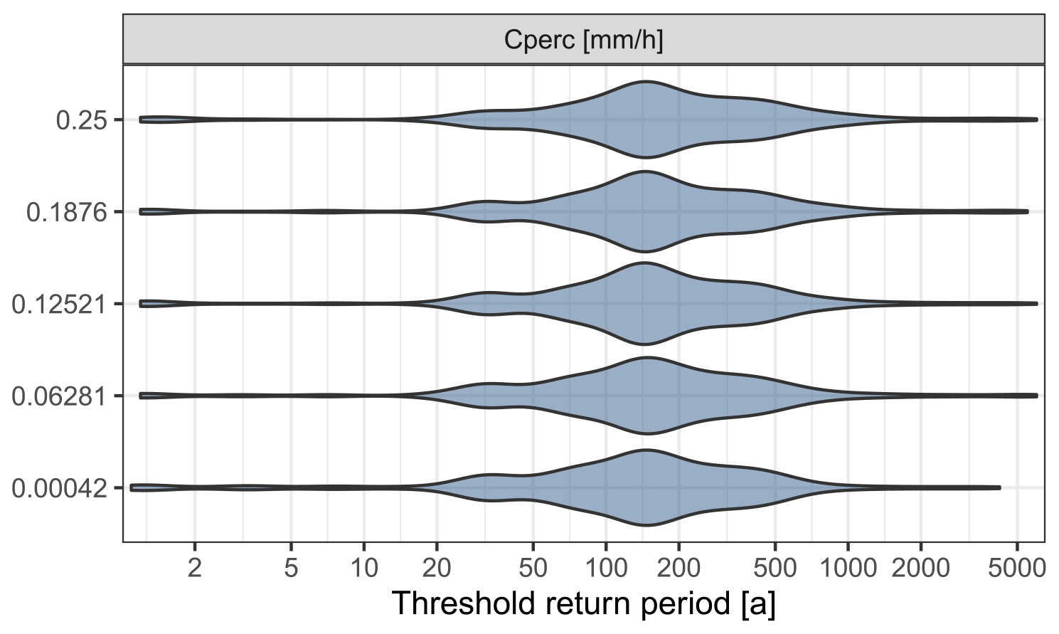
Figure B2 The relation of threshold return periods and the percolation rate from the upper to the lower subsurface storage (C_PERC). Results are based on 2310 model runs in which a threshold return period within 6000 years was estimated. The threshold return period describes beyond which return period the frequency curves of discharge and precipitation run in parallel on a log–log plot, i.e. beyond which return period the flood peak distribution is governed by the rainfall distribution.

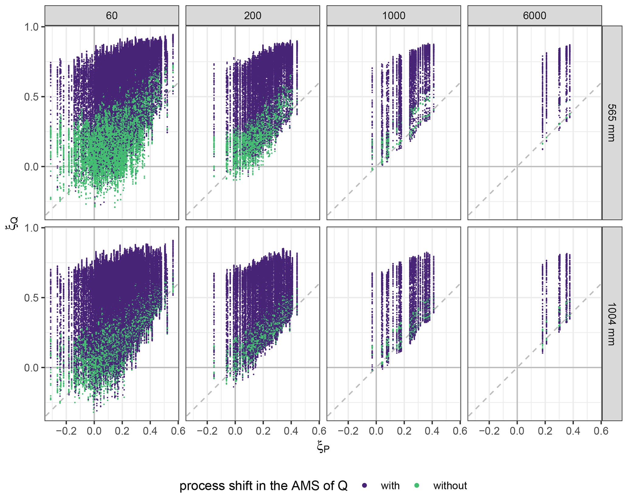
Figure B3 Shape parameters of generalized extreme value (GEV) distributions fitted to discharge series (ξ_Q) against GEV shape parameters of the precipitation series (ξ_P) that were used to simulate the discharge. Q is considered on an hourly scale, while P is considered on a 6-hourly scale. GEV distributions were fitted to annual maximum series (AMS) of 60, 200, 1000, and 6000 years. For each level of mean annual precipitation (565 and 1004 mm), results are based on 875 model runs of 6000 years – seven P series with different tail behaviour but the same MAP and 5³ different parameter sets in the rainfall–runoff model. An AMS of Q was classified as containing a process shift when for some but not all of the flood peak events a storage threshold was exceeded and an additional and faster runoff component was triggered.