A comprehensive uncertainty framework for historical flood frequency analysis: a 500-year-long case study

The value of historical data for flood frequency analysis has been acknowledged and studied for a long time. A specific statistical framework must be used to comply with the censored nature of historical data, for which only floods large enough to induce written records or to trigger flood marks are usually recorded. It is assumed that all floods which exceeded a given perception threshold were recorded as written testimonies or flood marks. Conversely, all years without a flood record in the historical period are assumed to have had a maximum discharge below the perception threshold. This paper proposes a binomial model that explicitly recognizes the uncertain nature of both the perception threshold and the starting date of the historical period. This model is applied to a case study for the Rhône River at Beaucaire, France, where a long (1816–2020) systematic series of annual maximum discharges is available along with a collection of 13 historical floods from documentary evidence over 3 centuries (1500–1815). Results indicate that the inclusion of historical floods reduces the uncertainty of 100- or 1000-year flood quantiles, even when only the number of perception threshold exceedances is known. However, ignoring the uncertainty around the perception threshold leads to a noticeable underestimation of flood quantile uncertainty. A qualitatively similar conclusion is found when ignoring the uncertainty around the historical period length. However, its impact on flood quantile uncertainty appears to be much smaller than that of the perception threshold.

1 Introduction

Flood frequency analysis (FFA) provides information on the magnitude and frequency of flood discharges. It is used to estimate the probability of flooding and manage the risk posed by floods to human health, the environment, the economy and cultural heritage (European Union, 2007). One of the main concerns in FFA is the difficulty of precisely estimating the parameters of the chosen distribution with discharge series of limited length (generally a few decades). This is particularly problematic when low-probability (e.g. an annual exceedance probability of 10⁻³ or 10⁻⁴) design floods are required to ensure the safety of people and hydraulic structures (Apel et al., 2004; Kjeldsen et al., 2014). Fortunately, sampling uncertainty can be reduced by providing additional information beyond the flood sample obtained from discharge monitoring stations during a systematic period. Such information can be temporal (e.g. historical data on ancient floods), regional (e.g. discharge data from similar catchments), causal (e.g. rainfall data) (Merz and Blöschl, 2008) or a combination of these (Macdonald and Sangster, 2017). This paper focuses on the treatment of historical data in FFA.

Historical data can take a variety of forms: they may be issued from testimonials (Pichard, 1995; Kjeldsen et al., 2014); flood marks (Parkes and Demeritt, 2016; Piotte et al., 2016; Engeland et al., 2020; METS, 2023; Renard, 2023); or palaeoflood reconstructions derived from various proxies, such as sedimentary deposits or riparian tree rings (Stedinger and Cohn, 1986; Benito et al., 2004; Dezileau et al., 2014; St. George et al., 2020; Engeland et al., 2020). Using historical data in FFA has a long history and is now a well-established practice. Benson (1950) and Hirsch (1987) first focused on plotting position formulas for historical floods. Various types of historical data can be incorporated in FFA by selecting an adequate likelihood function (Stedinger and Cohn, 1986; Kuczera, 1999). Parameter estimation is often performed in a Bayesian way using Markov chain Monte Carlo (MCMC) algorithms (Reis and Stedinger, 2005). Most recent studies emphasize the need to take full account of uncertainties (Neppel et al., 2010; Kjeldsen et al., 2014; Parkes and Demeritt, 2016; Shang et al., 2021; Sharma et al., 2022). Although discharges from the systematic period are generally better known than those from the historical period, they are still affected by uncertainties. However, those uncertainties are often neglected when using historical data. Only a few works propose taking them into account: Reis and Stedinger (2005) or Parkes and Demeritt (2016) consider discharge uncertainty during the systematic period via the use of a fixed percentage error, while Neppel et al. (2010) use unknown multiplicative errors.

Historical flood data are not systematic: only floods large enough to induce written records or to trigger flood marks are recorded. Such censored data can be analysed statistically thanks to the perception threshold concept (Gerard and Karpuk, 1979; Stedinger and Cohn, 1986). The assumption is that all floods exceeding this perception threshold were recorded, thus ensuring the completeness of the historical flood record above the threshold. As a corollary, the annual maximum flood discharge can be assumed to be smaller than the perception threshold for all years in the historical period with no recorded flood. It is possible, although not mandatory, to reconstruct the discharge of historical floods above the perception threshold via the use of hydraulic models (Lang et al., 2004; Neppel et al., 2010; Machado et al., 2015). In cases where such reconstruction is too complex, the sole knowledge of the number of floods that exceeded the perception threshold during the historical period can be exploited by means of a binomial distribution, as described by Stedinger and Cohn (1986) or Payrastre et al. (2011). This method highlights two key quantities in historical FFA that constitute the main focus of this paper: the perception threshold and the length of the historical period.

The perception threshold is an empirical concept that only takes a physical meaning in specific cases. The ideal situation corresponds to the availability of a cross-section that has not changed over time, with overflows always occurring above the same discharge and systematically leaving a trace in written records or on infrastructure (flood marks) as a result of the damage caused. In such a situation, expressing the perception threshold as a precisely estimated discharge value is feasible. However, its estimation can be undermined by several factors, such as a complex river geometry or a temporally varying perception of flood damage among the populations living adjacent to the river. In spite of such uncertainties, the perception threshold is assumed to be perfectly known in the vast majority of studies, although the sensitivity of results to the perception threshold is often explored (Stedinger and Cohn, 1986; Viglione et al., 2013; Macdonald et al., 2014; Payrastre et al., 2011; Parkes and Demeritt, 2016).

In the same way, the length of the historical period is generally considered to be perfectly known in the historical FFA methods in the literature. In principle, the historical period (or surveying period) should start on the date when the source of the historical information came into existence. However, it is generally assumed to start with the first known flood and to finish with the starting date of the systematic period. Prosdocimi (2018) showed that this leads to a systematic underestimation of the length of the historical period and, thus, proposed an unbiased estimator of the starting date of the historical period. However, this unbiased estimator is still treated as a known value in the subsequent FFA procedure, even though it is affected by considerable uncertainty.

This paper presents an FFA probabilistic model that (1) uses the number of times a perception threshold is exceeded over a historical period and (2) accounts for the uncertainty in discharges during the systematic period. The key originality of this model is to recognize the imperfectly known nature of both the perception threshold and the length of the historical period by making them parameters of the probabilistic model. The aim is to correctly assess the uncertainties in flood quantiles, based on historical information.

This FFA model and several variants are applied to a case study based on the Rhône River at Beaucaire, France, offering a very long systematic record (1816–2020, 205 years) with carefully determined discharge uncertainties. An uncertainty propagation chain developed by Lucas et al. (2023) accounts for errors on stage and gauging measurements as well as rating curve estimation. In a first step, the 205-year systematic record is artificially subsampled in order to mimic a typical mixed dataset containing about 50 years of systematic data and about 150 years of censored historical data. This allows for the testing of the FFA models on a real-world dataset, with the full 205-year systematic dataset providing a precise baseline against which comparisons can be made. The added value of precisely knowing the discharge of historical floods vs. only knowing the number of perception threshold exceedances is also explored. In a second step, the same FFA models are then applied to the 1816–2020 systematic record and a collection of historical floods during the 1500–1815 period (Pichard and Roucaute, 2014). The impact of the various sources of uncertainty in the quantile estimates is discussed.

This remainder of the paper is organized as follows: methods for historical FFA are introduced in Sect. 2; the available data are presented in Sect. 3, and their stationarity is verified; the FFA models are applied and compared using the artificially subsampled record on the 1816–2020 period in Sect. 4 and the entire dataset on the 1500–2020 period in Sect. 5; and, finally, Sect. 6 discusses some key results of this work, while Sect. 7 summarizes the study's main conclusions.

2 Probabilistic models

We first present how censored historical floods can be included into a probabilistic model (Sect. 2.1); following this, we move towards more specific models accounting for uncertainties (Sect. 2.2).

2.1 Standard treatment of censored data

2.1.1 Likelihood function

We assume that the annual maximum (AMAX) discharge Q during systematic and historical periods is an independent and identically distributed (i.i.d.) random variable that follows a generalized extreme value (GEV) distribution, with the respective location, scale and shape parameters θ= (μ, σ, ξ). When the shape parameter ξ is non-zero, the GEV cumulative distribution function (cdf) and the probability density function (pdf) are

$$\begin{array}{}\text{(1)}& \begin{array}{rl}& F\left(q;\mathit{\theta }\right)=\exp \left[-{\left(\mathrm{1}-\mathit{\xi }{\displaystyle \frac{q-\mathit{\mu }}{\mathit{\sigma }}}\right)}^{\mathrm{1}/\mathit{\xi }}\right]\\ & \text{and}\\ & f\left(q;\mathit{\theta }\right)={\displaystyle \frac{\partial F\left(q;\mathit{\theta }\right)}{\partial q}}={\displaystyle \frac{\mathrm{1}}{\mathit{\sigma }}}{\left(\mathrm{1}-\mathit{\xi }{\displaystyle \frac{q-\mathit{\mu }}{\mathit{\sigma }}}\right)}^{\mathrm{1}/\mathit{\xi }-\mathrm{1}}F\left(q;\mathit{\theta }\right).\end{array}\end{array}$$

Under this parameterization, a positive shape parameter (ξ > 0) corresponds to an upper-bounded distribution with quantiles lower than those of the corresponding Gumbel distribution. In the opposite case (ξ < 0), the distribution is heavy-tailed with above-Gumbel quantiles. The Gumbel case is obtained by continuity when ξ tends to zero.

The sample of AMAX discharges during the systematic period covering j years is noted $\mathit{q}={\left(q_t\right)}_{t=\mathrm{1},j}$. For the time being, discharges are supposed to be perfectly known and not affected by any uncertainty. The historical sample is made of k events that exceeded the perception threshold S over a period of n years. Therefore, the perception threshold was not exceeded over the remaining (n−k) years. The probability π of exceeding the threshold S can be written as follows:

$$\begin{array}{}\text{(2)}& \mathit{\pi }=\left(\mathrm{1}-F\left(S;\mathit{\theta }\right)\right)=\mathrm{1}-\exp \left[-{\left(\mathrm{1}-\mathit{\xi }{\displaystyle \frac{S-\mathit{\mu }}{\mathit{\sigma }}}\right)}^{\mathrm{1}/\mathit{\xi }}\right].\end{array}$$

It is assumed that k, the number of exceedances of the perception threshold, follows a binomial distribution ℬ(n,π). The likelihood function of a mixed sample of AMAX discharges q during the systematic period spanning j years and the number k of exceedances of the perception threshold S during the historical period spanning n years is as follows:

$$\begin{array}{}\text{(3)}& L\left(\mathit{\theta };\mathit{q},k\right)=\underset{\text{(a)}}{\underbrace{{\mathrm{\Pi }}_{t=\mathrm{1}}^{j}f(q_t;\mathit{\theta })}}\underset{\text{(b)}}{\underbrace{\left[\left(\begin{array}{c}n\\ k\end{array}\right)\left(F\right(S;\mathit{\theta }\left){)}^{n-k}\right(\mathrm{1}-F(S;\mathit{\theta }){)}^k\right]}}.\end{array}$$

Here, term (a) in Eq. (3) represents the likelihood for systematic data and term (b) in Eq. (3) represents the likelihood for historical data. By applying Bayes' formula, the posterior distribution $p\left(\mathit{\theta }\right|\mathit{q},k)$ of parameters θ given systematic and historical data is as follows:

$$\begin{array}{}\text{(4)}& p\left(\mathit{\theta }|\mathit{q},k\right)\propto L\left(\mathit{\theta };\mathit{q};k\right)p\left(\mathit{\theta }\right).\end{array}$$

The term p(θ) represents the prior distribution of the parameters and needs to be elicited before inference. The posterior distribution $p\left(\mathit{\theta }\right|\mathit{q},k)$ is explored using an MCMC sampling algorithm (Renard et al., 2006), leading to a representation of sampling uncertainty by means of r parameter vectors Θ= (θ₁, …, θ_r). The parameter vector $\widehat{\mathit{\theta }}$ that maximizes the posterior distribution is called “maxpost”. Thereafter, the prior distribution p(θ) of the GEV parameters will be as follows: a positive uniform distribution for μ and σ and a Gaussian distribution with a mean of zero and a standard deviation of 0.2 for ξ, as proposed by Martins and Stedinger (2000).

2.1.2 Starting date of the historical period

The starting date t^* of the historical period can be assessed by two methods. A first method proposed by Prosdocimi (2018) is based on the total number of exceedances of the perception threshold.

Let NE = NE_H (historical period) + NE_C (continuous period) denote the total number of exceedances of the perception threshold S recorded during NY years, with NY = NY_H (historical period) + NY_C (continuous period). Considering the date t₁ of the first known flood, which occurred (NY − 1) years before the end of the systematic period, Prosdocimi (2018) proposed choosing the starting date as follows:

$$\begin{array}{}\text{(5)}& t_{\left(\mathrm{Prosdocimi}\right)}^{*}=t_{\mathrm{1}}-\left(\mathrm{NY}-\mathrm{1}\right)/\mathrm{NE}.\end{array}$$

The idea behind this estimate is to start the historical period T_S years before the first known flood, where T_S is the return period of the perception threshold, estimated here as (NY − 1)/NE.

The second method is based on the Poisson process paradox (Feller 1971). It takes advantage of the fact that the expected duration between the last T-year event and current time is equal to the expected duration between current time and the next T-year event. In some cases, the historical period (including flood and no-flood information) starts before the date t₁ of the first known flood (e.g. at the creation of the service in charge of surveying floods or at the date of bridge construction where historical data are available). We denote this date using t_start and consider the difference (t₁−t_start) between these two dates. Without any knowledge of the return period T_S of the threshold but using the difference (t₁−t_start), we obtain the following:

$$\begin{array}{}\text{(6)}& t_{\left(\mathrm{Poisson}\right)}^{*}=t_{\mathrm{start}}-\left(t_{\mathrm{1}}-t_{\mathrm{start}}\right)=\mathrm{2}{t}_{\mathrm{start}}-t_{\mathrm{1}}.\end{array}$$

2.2 Models accounting for uncertainties

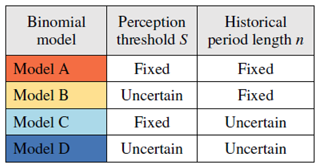
We first present a binomial model for the treatment of historical floods (a collection of historical floods larger than a perception threshold S) and systematic floods (AMAX discharges from a gauging station). This first model includes a propagation procedure of hydrometric uncertainties from the systematic period (Model A). We then extend this model to take into account the perception threshold uncertainty (Model B), the historical period length uncertainty (Model C), or both (Model D) (Table 1). A fifth model (Model E) considers the case in which historical flood discharges are known within an interval.

Table 1 Characteristics of the four binomial models.

2.2.1 Model A: binomial model for historical floods and propagation of systematic discharges uncertainties

In Eq. (3), the uncertainty of AMAX discharges for the systematic period is assumed to be negligible. As this uncertainty can reach 30 % at Beaucaire during the 19th century (see Sect. 3.1), it seems necessary to consider it. We use the propagation procedure accounting for both stage and rating curve uncertainties described by Lucas et al. (2023); this leads to s= 500 realizations of AMAX discharges: ${\left(q_t^{\left(i\right)}\right)}_{t=\mathrm{1},j;i=\mathrm{1},s}$. Each realization can be used to compute a posterior distribution with Eq. (4), and each posterior distribution can be explored with the MCMC sampler, with r= 500 MCMC simulations. This leads to a total of r×s parameter vectors ${\left({\mathit{\theta }}_p^{\left(i\right)}\right)}_{p=\mathrm{1},r;i=\mathrm{1},s}$, representing the combined effect of sampling uncertainty and hydrometric uncertainty from systematic data. The maxpost parameter vector is calculated using the maxpost sample of AMAX discharges. The model described above will be referred to as Model A. The propagation of hydrometric uncertainties from the systematic period described here will be carried out identically for all models defined in the following sections.

2.2.2 Model B: binomial model for historical floods, accounting for perception threshold uncertainty

A single perception threshold S for the entire sample is considered here. In order to take the imperfect knowledge of S into account, it is possible to consider it as an unknown parameter of the model and to represent this imperfect knowledge through a prior distribution. In the previous section, the perception threshold was already part of the model, but its value was assumed to be known, which is no longer the case here. Therefore, the left-hand side of Eq. (3) becomes $L\left(\mathit{\theta },S;\mathit{q},k\right)$ instead of $L\left(\mathit{\theta };\mathit{q},k\right)$, while the right-hand side remains unchanged. The posterior distribution of the parameters θ and S given the data is as follows:

$$\begin{array}{}\text{(7)}& p\left(\mathit{\theta },S|\mathit{q},k\right)\propto L\left(\mathit{\theta },S;\mathit{q},k\right)p\left(\mathit{\theta },S\right).\end{array}$$

This posterior distribution takes the hydrometric uncertainty from the systematic period, the sampling uncertainty and the perception threshold's uncertainty into account. This model will be referred to as Model B in the following sections. Note that it is necessary to specify a prior distribution for the perception threshold S that reflects the knowledge on this parameter, which is highly case-specific and can range from very imprecise to nearly known.

2.2.3 Model C: binomial model for historical floods, accounting for the uncertainty in the historical period length

The uncertainty in the number n of years constituting the historical period can be treated in the same way as described in the previous section for the threshold S. Generally, the ending date of the historical period is perfectly known, as it also corresponds to the start of the systematic recordings. However, the starting date t^* of the historical sample, from which all floods above the perception threshold are supposed to be recorded, is generally poorly known. The number n of years constituting the historical period can hence be treated as an unknown parameter of the probabilistic model. The perception threshold S is assumed to be perfectly known in this case. Therefore, the left-hand side of Eq. (3) becomes $L\left(\mathit{\theta },n;\mathit{q},k\right)$. The posterior distribution of the parameters θ and n given the data is as follows:

$$\begin{array}{}\text{(8)}& p\left(\mathit{\theta },n|\mathit{q},k\right)\propto L\left(\mathit{\theta },n;\mathit{q},k\right)p\left(\mathit{\theta },n\right).\end{array}$$

As previously stated, a prior distribution reflecting the partial knowledge of the length of the historical period has to be specified. The lack of knowledge on the length of the historical period is therefore taken into account in the model and has an impact on flood quantile uncertainty. This model will be referred to as Model C in the following sections.

2.2.4 Model D: binomial model for historical floods, accounting for both perception threshold and historical period length uncertainties

As the perception threshold S and the number n of years of the historical period are linked by definition (with a perception threshold being valid over a given duration), we finally consider a model that represents the lack of knowledge about both parameters. The left part of Eq. (3) becomes $L\left(\mathit{\theta },S;n;\mathit{q},k\right)$. The posterior distribution of the parameters θ, S and n given the data is as follows:

$$\begin{array}{}\text{(9)}& p\left(\mathit{\theta },S,n|\mathit{q},k\right)\propto L\left(\mathit{\theta },S,n;\mathit{q},k\right)p\left(\mathit{\theta },S,n\right).\end{array}$$

This model, for which S and n are uncertain, will be called Model D in the following sections.

2.2.5 Model E: considering historical flood discharges within intervals

In some cases, the discharge of historical floods above the perception threshold can be reconstructed and taken into account in the probabilistic model (e.g. Stedinger and Cohn, 1986). As such reconstructions are typically obtained by means of hydraulic models affected by large uncertainties, it is also useful to consider that the reconstructed discharges are not perfectly known but lie within intervals. Several examples of such models exist in the literature (e.g. Payrastre et al., 2011, or Parkes and Demeritt, 2016). The corresponding likelihood can be written as follows:

$$\begin{array}{}\text{(10)}& \begin{array}{rl}L(\mathit{\theta };\mathit{q},\mathit{y},k)& ={\prod }_{t=\mathrm{1}}^{j}f(q_t;\mathit{\theta }){\prod }_{i=\mathrm{1}}^k\left[F\right(y_i^{\sup };\mathit{\theta })\\ & -F(y_i^{\inf };\mathit{\theta })\left]\right(F(S;\mathit{\theta }){)}^{n-k},\end{array}\end{array}$$

where q_t corresponds to the j floods of the systematic period and y_i corresponds to the k floods of the historical period whose discharge values lie within the interval $\left[y_i^{\inf },y_i^{\sup }\right]$. The posterior distribution of the model is as follows:

$$\begin{array}{}\text{(11)}& p\left(\mathit{\theta }|\mathit{q},\mathit{y},k\right)\propto L\left(\mathit{\theta };\mathit{q},\mathit{y},k\right)p\left(\mathit{\theta }\right).\end{array}$$

Here, the perception threshold and the length of the historical period are assumed to be perfectly known. This model will be referred to as Model E in the following sections. The quantiles can be compared with the results of the binomial models, for which only the number k of perception threshold exceedance S is known.

3 Case study: the Rhône River at Beaucaire

3.1 Discharge data over 5 centuries

We first consider the 205-year-long daily discharge series of the Rhône River at Beaucaire, France, from 1816 to 2020 (catchment area of 95 590 km²). Daily stage measurements started in 1816. The gauging station was used until the construction of the Vallabrègues hydroelectric scheme in 1967, which led to the derivation of a part of the discharge. Consequently, the gauging station was relocated 2 km downstream, in order to measure the total discharge (i.e. downstream from the restitution of the diverted discharge). The Vallabrègues Dam has no impact on the discharge at the station, as it has a very limited storage capacity and is opened during floods to cancel the backwater effect that it creates for low flows. A set of 500 realizations of AMAX floods from 1816 to 2020 is available from Lucas et al. (2023), accounting for several sources of hydrometric uncertainty. The estimated 95 % discharge uncertainty varies from 30 % (19th century) to 5 % (1967–2020).

Secondly, a collection of historical flood testimonies from 1500 to 1815 is available from the HISTRHÔNE database (Pichard and Roucaute, 2014). We focus on the 13 extreme floods (in 1529, 1548, 1570, 1573, 1674, 1694, 1705, 1706, 1711, 1745, 1755, 1801 and 1810), referenced as C4-class events: “extreme flood and inundation”. This ensemble is considered to be a comprehensive survey of the most damaging floods of the historical period. The perception threshold S is about 9000 m³ s⁻¹ according to Pichard et al. (2017). Figure 1a shows the available flood discharge sample with the corresponding uncertainties. Note that we used a very uncertain prior for the perception threshold in order to more clearly highlight its impact.

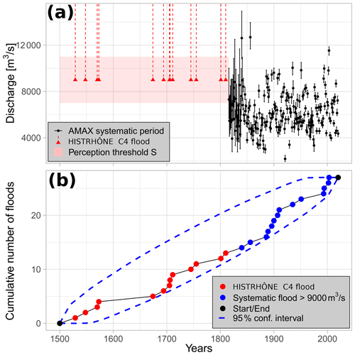
Figure 1 (a) The Rhône River at Beaucaire, AMAX flood discharges with their 95 % uncertainty intervals (1816–2020, systematic period; Lucas et al., 2023) and C4-class floods from 1500 to 1815 (HISTRHÔNE database). (b) The cumulative number of C4-class floods and peak-over-threshold floods (systematic period) with the 95 % Poisson process confidence interval.

3.2 Stationarity tests

As the probabilistic models described in Sect. 2 assume that AMAX values are independent and identically distributed (i.i.d.), statistical tests should be applied to check the stationarity of both systematic and historical periods.

3.2.1 Systematic data

The Pettitt step-change test (Pettitt, 1979) and Mann–Kendall trend test (Mann, 1945; Kendall, 1948) were applied to the maxpost series of AMAX discharges during the 1816–2010 period. The respective p values of 0.15 and 0.4 indicate no significant change. The segmentation procedure proposed by Darienzo et al. (2021) was also applied, as it allows one to account for the uncertainty around AMAX discharges. This procedure indicates that the optimum number of segments is equal to 1, confirming the absence of significant change.

3.2.2 Historical data

The historical data used here (13 extreme C4-class floods) can be interpreted as peak-over-threshold (POT) values, as they correspond to all floods that exceeded the perception threshold S. Moreover, there is no year with more than one C4-class flood during the 1500–1815 period. AMAX values from the continuous period larger than 9000 m³ s⁻¹ can also be viewed as POT values, as the 14 largest values from the daily record (in 1840, 1856, 1886, 1889, 1896, 1900, 1907, 1910, 1935, 1951, 1993, 1994, 2002 and 2003) are from different years. Assuming that the number of occurrences of POT discharges follows a Poisson process, it is possible to compute a confidence interval for the cumulative number N_t of POT values during a period 0–t (Lang et al., 1999) and to verify that the experimental curve is inside the limits of the interval. The Poisson test is applied to the whole period 1500–2020, using POT values from both historical and systematic periods (1500–1815 and 1816–2020). Figure 1b shows that the experimental curve is within the 95 % confidence interval. Hence, the whole sample can be considered to be stationary.

4 Flood frequency analysis on the 1816–2020 period

4.1 Subsampled datasets

In this section, the GEV distribution fitted with AMAX discharges from the 1816–2020 period (including the propagation of hydrometric uncertainty described in Sect. 2.2, Model A) is used as a reference and is referred to as “AMAX long”. It can be compared with GEV distributions estimated with subsampled data, where only part of the available information is used:

• The first subsample contains a short sample of AMAX discharges during the 1970–2020 period, referred to as “AMAX short”. It corresponds to the typical length of hydrometric series in France, about 50 years of record, leading to a large extrapolation of the estimated distribution towards large quantiles (100-year or 1000-year return period).

• The second subsample is a mixed sample, with AMAX discharges for the 1970–2020 period and a collection of historical values for the 1816–1969 period, referred to as “Mixed A”–“Mixed E”, according to the model used. A perception threshold S= 9000 m³ s⁻¹ leads to a collection of 10 historical floods. When using Model B (or Model D), we consider a vague normal prior distribution on the perception threshold: N(9000;2000), with 2000 being the standard deviation. When using Model C (or Model D), we consider a uniform prior distribution on the starting date of the historical period: U[1316;1816], corresponding to a large uncertainty (500 years).

Results with systematic data only (AMAX long and AMAX short) or with a mixed sample (AMAX short + 10 historical floods) are presented for the estimation of Q₁₀₀ and Q₁₀₀₀ floods (Fig. 2b), parameters (ξ, S and t^*) (Table 2) and GEV distributions (Fig. 2a). The plotting position formula proposed by Hirsch (1987) for a mixed sample with AMAX values from a continuous period and historical discharges larger than a perception threshold is applied. The Appendix provides a procedure for a case in which historical flood discharges are unknown, using only exceedances of the threshold.

Table 2 Maxpost estimation ± the posterior standard deviation (expressed as a percentage) for Q₁₀₀ and Q₁₀₀₀ floods and the ξ, S and t^* parameters (1816–2020 period).

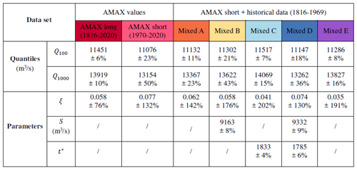
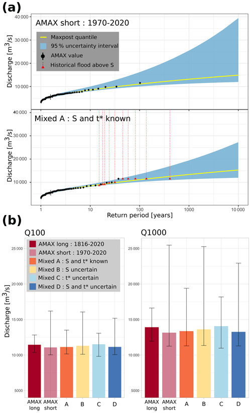
Figure 2 (a) GEV quantiles with their 95 % credibility intervals, displaying an example of two different models and datasets: the GEV model on AMAX values (AMAX short 1970–2020) and the binomial Model A on a mixed sample (1816–2020). (b) The Q₁₀₀ and Q₁₀₀₀ floods with their 95 % credibility intervals displayed as error bars. AMAX long refers to the sample for the 1816–2020 period; AMAX short refers to the sample for the 1970–2020 period; and Mixed A, B, C and D refer to a mixed sample (“historical” floods in the 1816–1969 period and AMAX 1970–2020) for various statistical models.

4.2 Value of adding historical information from the 1816–1969 period

Unsurprisingly, when the length of the systematic record (∼ 50 years) is too short compared with the target return period (∼ 100 or 1000 years), the results are highly uncertain (AMAX short in Fig. 2). A binomial model exploiting historical flood events notably reduces uncertainty when the perception threshold S is known (Mixed A and Mixed C in Fig. 2b), although not achieving the precision obtained with 205 years of systematic records (AMAX long in Fig. 2b). Accounting for the uncertainty in the threshold S (Mixed B and Mixed D in Fig. 2b) increases the uncertainty in flood quantiles and nearly annihilates the interest of historical flood occurrences.

The main part of the uncertainty comes from the estimation of the shape parameter ξ, which governs the behaviour of the tail of the distribution. Note that all of the estimates are close to zero and slightly positive (Table 2), corresponding to an upper-bounded distribution. As might be expected, the estimate of parameter ξ is much more precise with a long series (AMAX long) of 2 centuries than with a short series (AMAX short) of 5 decades. The use of historical data through a binomial model is not very efficient with respect to reducing uncertainty in the shape parameter ξ (Table 2). Overall, the maxpost estimate of the Q₁₀₀ and Q₁₀₀₀ quantiles are very close for all models (Fig. 2b). In the next sections, the impact of accounting for the uncertainties in the perception threshold S and the starting date t^* of the historical period is assessed in more detail.

4.3 Impact of considering that the perception threshold is uncertain

The use of Model B reflects a lack of knowledge on the perception threshold, which becomes a parameter of the model. Figure 2b shows that the quantile uncertainty estimated with Model B is much greater than with Model A and that it is close to the one obtained with systematic data only (AMAX short). Therefore, poor knowledge of the perception threshold has major consequences for the quantile estimates, as it greatly reduces the value of using historical occurrences. The true value of the perception threshold is S= 9000 m³ s⁻¹. The prior and posterior distributions of the threshold S are shown in Fig. 3a. It can be seen that the posterior estimate for Model B (9163 m³ s⁻¹) is close to the true value (9000 m³ s⁻¹) and that the model has effectively improved the knowledge of the threshold compared with the prior distribution N(9000;2000). The posterior uncertainty in the shape parameter ξ for Model B is greater than that of Model A and, thus, becomes almost identical to that of AMAX short (Table 2). In real-world case studies, specifying a more precise prior should limit this impact and should, hence, be considered to be a priority objective for historical FFA.

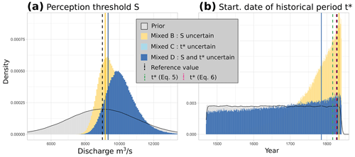
Figure 3 Prior and posterior distributions of (a) the perception threshold S and (b) the starting date t^* of the historical period (1816–2020 period). The solid vertical lines represent the maxpost estimate of the parameter for each of the models, whereas the dashed black lines represent the reference values (S= 9000 m³ s⁻¹ and $t^{*}=$ 1816). The dashed vertical green and pink lines in panel (b) represent the estimates of t^* from Eqs. (5) and (6), respectively.

4.4 Impact of considering that the historical period length is uncertain

Model C is used to represent the lack of knowledge on the length of the historical period. In Fig. 2b, the maxpost quantile estimates for Model C have slightly higher values than the estimates for Model A. This may be due to the underestimation of the length of the historical period, as can be seen in Fig. 3b. The maxpost date is 1833, whereas the series actually begins in 1816. This 17-year underestimation can be explained by a greater frequency of floods above the threshold S during the systematic period (4 floods during 50 years, i.e one exceedance every 12.5 years) than during the historical period (10 floods during 153 years, i.e one exceedance every 15 years). This imbalance is probably due to sampling variability, as no break or trend was detected by the stationarity tests in Sect. 3.2. The posterior distribution of the starting date t^* for Model C (Fig. 3b) is much more precise than the prior distribution and is strongly asymmetric. The uncertainty around the quantiles estimated by Model C is very similar to that estimated by Model A (Fig. 2b), as is the distribution of the shape parameter (Table 2). Overall, these results indicate that a poor knowledge of the length of the historical period has less impact on the precision of quantile estimates than poor knowledge of the perception threshold.

4.5 Impact of considering that both the perception threshold and the historical period length are uncertain

Model D assumes that both S and n are uncertain in the probabilistic model. The maxpost quantiles estimated in Fig. 2b are close to the reference values. In contrast, the width of the credibility interval is large and lies between that of Model B and Model C. Although the estimate is more accurate than with a short series (AMAX short), it remains very imprecise for the 1000-year flood. Figure 3 helps to understand the origin of this large uncertainty. The posterior distribution of the perception threshold S, although with a maxpost value (9332 m³ s⁻¹) close to the true value (9000 m³ s⁻¹), is very imprecise with a large standard deviation (883 m³ s⁻¹). The perception threshold S appears to be slightly less precisely estimated than with Model B (Table 2), with a posterior standard deviation of 9 % and 8 %, respectively. The starting date of the historical period is even more difficult to estimate, particularly in comparison with the estimate from Model C. It can be seen that the posterior distribution t^* of Model D is very similar to the prior uniform distribution (Fig. 3b), although it is slightly asymmetrical and shows a maximum not far from the true value (the year 1816). However, the flood discharge quantiles are less uncertain for Model D than for Model B. The precise reasons for this are unclear at this stage but might be due to some correlations between parameters. In particular, the Pearson correlation coefficient ρ is equal to 0.44 and 0.42 between the length of the historical period n and the perception threshold S and between the perception threshold S and the shape parameter ξ, respectively.

4.6 Value of estimating the peak discharge of the historical flood

Binomial models A, B, C and D only use information on the number of times k that a perception threshold S is exceeded over a period of n years. The discharge of historical floods that have exceeded the threshold is therefore ignored. Model E allows peak discharge estimates (with uncertainty) to be taken into account. The results are shown in Fig. 4. There is a reduction in uncertainty of around 25 % for Q₁₀₀₀ with Model E compared with binomial Model A (posterior standard deviations of 2255 and 3019 m³ s⁻¹, respectively). However, the uncertainty in Model E remains around 65 % greater than that of the GEV 1816–2020 model for Q₁₀₀₀. Although it is not a necessary condition for using historical data, knowledge of the discharge of historical floods does reduce the uncertainty around extreme quantiles. However, these results are only valid for the perception threshold S used here, which has a return period of about 15 years (with 14 exceedances during 205 years). Stedinger and Cohn (1986) and Payrastre et al. (2011) showed that the difference in uncertainty between the results of these two types of models tends to decrease as the return period of the perception threshold increases towards 50 years or so, until it becomes negligible above this magnitude. This encourages the use of the number of exceedances of a perception threshold when it is not possible to obtain better information on historical floods.

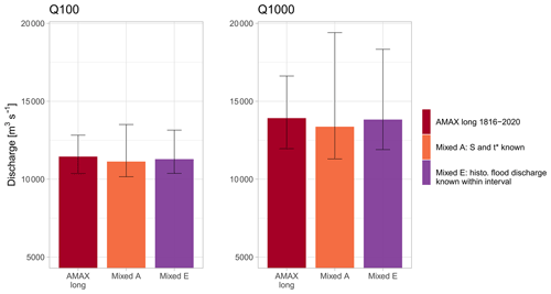
Figure 4 The Q₁₀₀ and Q₁₀₀₀ floods with their 95 % credibility intervals displayed as error bars. AMAX long refers to an annual maximum sample for the 1816–2020 period; Mixed refers to a mixed sample (“historical” floods in the 1816–1969 period and AMAX 1970–2020). Model A uses only the number of times that the perception threshold has been exceeded, whereas Model E considers the peak discharge (and its uncertainty) of each historical flood that exceeded threshold S. Perception threshold S and the start date of historical period t^* are considered perfectly known (models A and E).

5 Flood frequency analysis on the 1500–2020 period

In the previous section, we used a synthetic case study from a 205-year systematic record (1816–2020), which gives a baseline to compare the performance of five proposed models (A, B, C, D and E) with known parameters (S and n). The systematic record has been artificially subsampled into a mixed dataset that contains 51 years of systematic data (1970–2020) and 154 years of censored historical data larger than a known perception threshold (1816–1969). In this section, binomial models (A, B, C and D) are applied to a 500-year-long case study, using the 205-year systematic record (1816–2020) and a collection of historical floods from HISTRHÔNE database (1500–1815). This time, S and n are not perfectly known.

5.1 Prior on the perception threshold S and the starting t^* of the historical period

Binomial models A, B, C and D are now applied to a mixed sample over the period from 1500 to 2020, with AMAX values for the systematic period from 1816 to 2020 and occurrences of flood above the perception threshold for the historical 1500–1815 period. The perception threshold and the starting date of the historical period are not known precisely, and a first analysis is carried out with vague priors, with $S\sim N\left(\mathrm{9000};\mathrm{2000}\right)$ and $t^{*}\sim U\left[\mathrm{1129};\mathrm{1529}\right]$. By definition, the historical period begins, at the latest, on the date of the first known historical flood in 1529. The lower limit of the uniform distribution is arbitrarily set 400 years before the date of the first historical flood in order to represent the lack of knowledge on t^*.

A second analysis will refine the results of Model D, with more accurate prior estimates of S and t^* used for the historical 1500–1815 period, based on information of the systematic 1816–2020 period. The application of Model D with these more informative priors will be referred to as Model D^*. Figure 5 cross-references C4-class (extreme) floods occurring between 1816 and 2000 according to the HISTRHÔNE database (Pichard et al., 2017) and the estimated AMAX discharge values on the same period (Lucas et al., 2023). A total of 5 amongst 14 C4-class floods are below the threshold S= 9000 m³ s⁻¹. Even accounting for discharge uncertainty, three C4-class floods are still fully below the threshold S. As the flood ranking of the HISTRHÔNE database is based on physical impacts (e.g. morphologic river changes and city submersions), it is not possible to have a direct match between C4-class floods and an exact discharge threshold. We refine the prior distribution N(9000;500), with a standard deviation of 500 m³ s⁻¹ (instead of 2000 m³ s⁻¹ with Model D). No C4-class flood is fully below the 95 % prior 8000–10 000 interval.

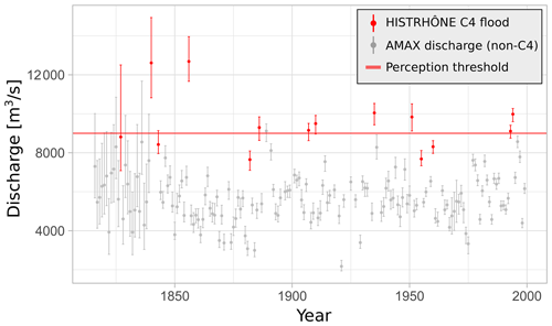
Figure 5 AMAX flood discharges (1816–2000) from Lucas et al. (2023) (in grey) cross-referenced with C4-class floods from the HISTRHÔNE database (in red). The horizontal line corresponds to the estimated perception threshold S= 9000 m³ s⁻¹.

Considering the 13 C4 floods in the HISTRHÔNE database (1500–1815) and the 14 floods higher than a threshold S= 9000 m³ s⁻¹ during the 1816–2020 period, we have two possible estimates of the starting date t^* of the historical period:

• $t_{\left(\mathrm{Prosdocimi}\right)}^{*}=$ 1511 (from Eq. 5), with knowledge of the date of the first known flood (t₁= 1529), the total number of threshold exceedances (NE = 13 (C4 floods) + 14 (AMAX > S) = 27) and the total number of years (NY = 2020–1529 = 491 years);

• $t_{\left(\mathrm{Poisson}\right)}^{*}=$ 1471 (from Eq. 6), with knowledge of the starting date of the surveying period (t_start= 1500).

We refine the prior distribution of t^* as U[1471;1529], with a width of 58 years (instead of 400 years with Model D).

5.2 Results with a vague prior on the perception threshold and the historical period length

Results with systematic data only (AMAX) on the 1816–2020 period or with a mixed sample (AMAX + 13 historical floods) on the 1500–2020 period are presented for the estimation of Q₁₀₀ and Q₁₀₀₀ floods (Fig. 6) and parameters (ξ, S and t^*) (Table 3).

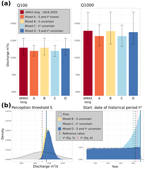
Figure 6 (a) The Q₁₀₀ and Q₁₀₀₀ floods with their 95 % credibility intervals displayed as error bars. AMAX long refers to the annual maximum sample for the 1816–2020 period; Mixed A, B, C and D refer to a mixed sample (“historical” floods in the 1500–1815 period and AMAX for 1816–2020) for various statistical models. (b) Posterior distribution of (left) the perception threshold S and (right) the starting date t^* of the historical period (1500–2020 period). The solid vertical lines represent the parameter maxpost estimates for each model, whereas the dashed black lines represent the reference values (S= 9000 m³ s⁻¹ and $t^{*}=$ 1500). The dashed vertical green and pink lines (right) represent the estimates of t^* by Eqs. (5) and (6), respectively.

Table 3 Maxpost estimation ± the posterior standard deviation (expressed as a percentage) for Q₁₀₀ and Q₁₀₀₀ floods and the ξ, S and t^* parameters (1816–2020 and 1500–2020 periods).

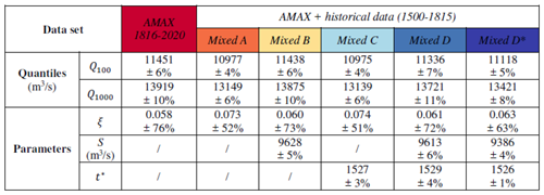
The results with a mixed sample for the 1500–2020 period show that the uncertainty in Q₁₀₀ and Q₁₀₀₀ floods (Fig. 6a) is lower than with AMAX values for the 1816–2020 period for models assuming a known perception threshold (models A and C). For these two models (Model A and Model C), the maxpost quantiles are also slightly lower (by around 5 %) than with AMAX values for the 1816–2020 period (Fig. 6a). As for the subsamples in Sect. 4, this suggests that poor knowledge of the perception threshold (models B and D) is more detrimental to the precision of estimated quantiles than poor knowledge of the historical period length (models C and D). In particular, these differences can be explained by looking at the posterior distributions of the parameters S and t^* (Fig. 6b).

The posterior standard deviations for the perception threshold (models B and D) are relatively small (around 500 m³ s⁻¹ for both models) and the distributions mostly lie above the prior value of 9000 m³ s⁻¹ (maxpost values around 9600 m³ s⁻¹; Table 3). The starting date t^* of the historical period is more precisely estimated with Model C than with Model D, whose posterior distribution is very close to the prior distribution. For both models, the maxpost estimates of t^* are almost 30 years higher than the assumed value of 1500. In particular, the posterior distribution for Model C shows a maximum for the year 1529, which corresponds to the date of the first flood in the sample.

This trend towards a higher threshold and a shorter historical period could be a symptom of the non-exhaustiveness of the extreme floods (C4 category) in the HISTRHÔNE database, despite the fact that the stationarity hypothesis of the Poisson test over the 1500–2020 period was not rejected (Fig. 1b). Once again, we can compare the rate of occurrence of floods above the threshold S= 9000 m³ s⁻¹ for each of the two samples. For the historical sample, 13 floods were observed over 316 years, i.e. one exceedance every 24 years. For the systematic sample, there were 14 floods over a period of 205 years, i.e. one exceedance every 15 years. This larger frequency of S exceedances of the systematic period, whether due to sampling variability, climatic variability or the non-exhaustiveness of the historical data, leads to the estimation of a higher perception threshold and/or a shorter historical period length.

5.3 Refining prior distributions of the perception threshold and the historical period length

The previous analysis is refined using narrower prior distributions of the perception threshold S and the starting date t^* of the historical period. A comparison of the binomial models D and D^* and the AMAX GEV 1816–2020 model is presented in Fig. 7a. It can be seen that the uncertainty in the quantiles is about 15 % lower than the reference for Q₁₀₀ and Q₁₀₀₀. Maxpost estimates are also reduced by approximately 3 % for both return periods. Therefore, the use of historical floods appears relevant to reduce the uncertainty in the quantiles, even in the case where S and n are uncertain. It can also be noted that the elicitation of more informative priors (see Falconer et al., 2022, for a methodological review) reduced the standard deviation of the posterior distribution for Q₁₀₀₀ by about 25 % (comparison of Model D with vague priors for S and t^* and Model D^* with refined priors).

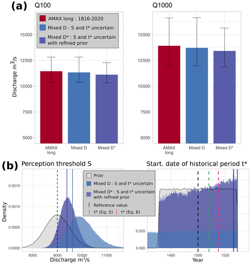
Figure 7 (a) The Q₁₀₀ and Q₁₀₀₀ floods with their 95 % credibility intervals displayed as error bars. AMAX long refers to an annual maximum sample for the 1816–2020 period; Mixed D^* refers to a mixed sample (“historical” floods in the 1500–1815 period and AMAX for 1816–2020), with refined priors for S and t^*. (b) Posterior distributions of (left) the perception threshold S and (right) the starting date t^* of the historical period for the two mixed models, Mixed D and Mixed D^*. The solid vertical lines represent the maxpost estimate of the parameter for each of the models, whereas the dashed black lines represent the reference values (S= 9000 m³ s⁻¹ and $t^{*}=$ 1500).

The posterior distributions of S and t^* are shown in Fig. 7b. Once again, the posterior distribution of the perception threshold is shifted towards values higher than the assumed value of 9000 m³ s⁻¹, with a maxpost threshold at 9386 m³ s⁻¹. The posterior distribution of t^* is again very close to the prior distribution, with a slightly higher density for the years close to the date of the first flood. Here, the maxpost estimate of t^* is 1526, i.e. a historical period length that is 26 years shorter than expected. Therefore, doubt remains as to the completeness of the historical sample or the inter-sample stationarity as described in the previous section.

6 Discussion

6.1 Main findings for the 1816–2020 period

By using the probabilistic models described in Sect. 2 on an artificially degraded sample whose characteristics are well known, it is possible to assess the impact of limited knowledge of the perception threshold S and the length n of the historical period on the estimation of extreme quantiles. The results show that poor knowledge of the perception threshold has a greater impact than poor knowledge of the historical period length. Even if the maxpost estimates of the perception threshold for models B and D are close to the true value (9000 m³ s⁻¹), the uncertainty resulting from determining the threshold has a strong impact on quantile uncertainty. Furthermore, the estimation of the historical period length in the case of Model C is also quite imprecise, but this has little impact on the uncertainty in the results when compared with those of Model A. The comparison of Model A, for which only the number of exceedances of the perception threshold is known, with Model E, for which the discharge of historical floods is known within an uncertainty interval, demonstrated the value of reconstructing the discharge of each historical flood.

Finally, the results for the 1816–2020 period suggest that the quantile uncertainty may be underestimated when the perception threshold and the historical period length are unduly considered to be perfectly known. The models proposed in this paper allow us to account for imperfect knowledge when estimating extreme quantiles.

6.2 Main findings for the 1500–2020 period

Application of the binomial Model D to a mixed sample with the discharge estimate of AMAX values for the systematic 1816–2020 period and a collection of 13 historical floods from 1500 to 1815 allows the uncertainty around the perception threshold S and the historical period length to be considered. Priors of Model D were refined, in order to have a more realistic assessment of threshold S and the starting date t^* of the historical period. This refined model, called Model D^*, gives the following results:

• Despite the fact that the available AMAX flood series for the 1816–2020 period is really long (205 years), it is possible to reduce the uncertainty in the flood quantiles (Fig. 7a) by adding information on 13 exceedances of a threshold S= 9000 m³ s⁻¹ during 3 prior centuries (period 1500–1815) and prior knowledge about S and t^*.

• The refinement of the prior distributions for the threshold S and the starting date t^* with Model D^* gives a more precise assessment of flood quantiles than with Model D (Fig. 7a). The posterior standard deviation (expressed as a percentage) of the Q₁₀₀₀ quantile decreases from 11 % to 8 % (Table 3). In both cases, considering the perception threshold S to be uncertain has much more of an impact on the uncertainty in the results than considering a lack of knowledge about the length of the historical period.

• The combination of an increased perception threshold (S_maxpost= 9386 m³ s⁻¹ vs. S_prior= 9000 m³ s⁻¹) and a reduced span of the historical period ($t_{\mathrm{maxpost}}^{*}=$ 1526 vs. $t_{\mathrm{prior}}^{*}=$ 1500) may be a symptom of the non-exhaustiveness of floods in the historical samples in the HISTRHÔNE database, even though no non-stationarity of the frequency of floods was detected (Fig. 1b). As the historical flood inventory is based on physical impacts, it may be sensitive to some changes in land settlement and flood protection.

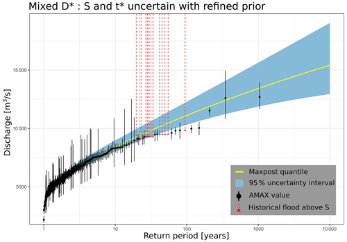
• The flood distribution and 95 % credibility interval of Model D^* are represented in Fig. 8. AMAX values are reported with their uncertainty (from 5 % to 30 %), and historical floods are reported as exceedances. Information on floods during 3 prior centuries (1500–1815) reduces the level of extrapolation towards extreme floods (flood of record has a plotting position around the 1000-year return period in Fig. 8, rather than a 400-year return period, as shown in Fig. 2a, for the 1816–2020 period).

Figure 8 Flood distribution and the 95 % confidence interval of Model D^* (mixed sample: systematic period 1816–2020 + 13 historical exceedances on 1500–1815, refined prior on S and t^*). The experimental distribution is shown in black (AMAX values) or red (exceedances of the perception threshold).

7 Conclusion

This paper proposes binomial models for the inclusion of historical data into FFA; these models explicitly recognize the uncertain nature of both the perception threshold and the starting date of the historical period.

The models are first tested with a 205-year-long series of AMAX values for the outlet of the Rhône River at Beaucaire, France. The time series has been artificially subsampled in order to mimic a historical context, considering AMAX values for a 50-year period (1970–2020) and a collection of 10 “historical” floods during the 1816–1969 period. The estimated quantiles were compared with estimates from a GEV model with AMAX values for the entire period (1816–2020). Considering that the perception threshold is perfectly known when this is not the case can lead to a significant underestimation of the uncertainty in flood quantiles. This also holds for the length of the historical period, although to a much lesser extent. In the case of this subsample, the use of historical data makes it possible to reduce the uncertainty in the quantiles compared with the sole use of the short systematic sample (1970–2020), considering uncertainties in the threshold S and the starting date t^* of the historical period. The binomial model estimate with known S and t^* (Model A) was then compared to an estimate for which historical flood discharges are known within an interval (Model E). In Beaucaire, the use of the historical flood discharges turned out to be slightly more informative than the use of the sole number of exceedances of the perception threshold.

The paper also presents the results of the binomial model with a mixed sample of 205 AMAX values (1816–2020 period) and 13 occurrences of historical floods (1500–1815 period). The addition of historical information for 3 centuries reduces the uncertainty in the Q₁₀₀ and Q₁₀₀₀ flood quantiles (about 15 %), despite only the number of exceedances being known. However, some doubts remain about the completeness of the historical sample, as the posterior estimation of S and t^* are larger than the prior.

The stationarity hypothesis may be challenged by climatic variability at Beaucaire, as trends in flood magnitudes have been identified in several regions of Europe (Hall et al., 2014; Blöschl et al., 2020) and France (Giuntoli et al., 2019). To date, there are no rules in France for accounting for the impact of climate change on flood risk estimates. However, it is still possible to integrate temporal changes in climate processes or watershed characteristics into the probabilistic model itself, as increasingly described in the literature (see Salas et al., 2018, for an overview). It is also important to note that, although outside of the FFA scope, such long series remain interesting for the study of the long-term variability in floods over several centuries and of their value for risk awareness and memory.

Appendix A: Plotting position for unknown historical floods

The exceedance probability of the ith value q(i) of a sample (q(1) ≥ … ≥q(N)), sorted by decreasing value, is as follows:

$$\begin{array}{}\text{(A1)}& {p^{\prime }}_i=\mathrm{Prob}\left[Q>q\left(i\right)\right]={\displaystyle \frac{i-a}{N+\mathrm{1}-\mathrm{2}a}},\end{array}$$

using, for example, a=  0.44, the optimum value for a Gumbel distribution (Cunnane, 1978).

Hirsch (1987) proposed splitting a mixed sample, formed by $\left(q_{\mathrm{1}},\mathrm{\dots },q_{{\mathrm{NY}}_{\mathrm{C}}}\right)$ AMAX values during NY_C years (continuous period) and NE_H historical values larger than a perception threshold S during NY_H years (historical period), into two subsamples:

• NE exceedances of the threshold S for the whole period (divided into NE_H and NE_C exceedances for the historical and continuous periods, respectively), during NY years, with NY = NY_H+ NY_C years,

  $$\begin{array}{}\text{(A2)}& \begin{array}{rl}\mathrm{Prob}\left[Q>q\left(i\right)\right]& =\left({\displaystyle \frac{\mathrm{NE}}{\mathrm{NY}}}\right){p^{\prime }}_i=\left({\displaystyle \frac{\mathrm{NE}}{\mathrm{NY}}}\right){\displaystyle \frac{i-\mathrm{0.44}}{\mathrm{NE}+\mathrm{0.12}}}\\ & i=\mathrm{1},\mathrm{NE};\end{array}\end{array}$$

• floods lower than S for the continuous period,

  $$\begin{array}{}\text{(A3)}& \begin{array}{rl}\mathrm{Prob}\left[Q>q\left(i\right)\right]& =\left({\displaystyle \frac{\mathrm{NE}}{\mathrm{NY}}}\right)\\ & +\left(\mathrm{1}-{\displaystyle \frac{\mathrm{NE}}{\mathrm{NY}}}\right){\displaystyle \frac{(i-\mathrm{NE})-\mathrm{0.44}}{{\mathrm{NY}}_{\mathrm{C}}-{\mathrm{NE}}_{\mathrm{C}}+\mathrm{0.12}}}\\ & i=\mathrm{NE}+\mathrm{1},{\mathrm{NY}}_{\mathrm{C}}+{\mathrm{NE}}_{\mathrm{H}}.\end{array}\end{array}$$

In the current case study, as the discharge of historical floods is not known (only threshold exceedance), it is not possible to rank all values of the mixed sample. A way to circumvent this problem is to randomly rank the historical unknown floods amongst the NE_C floods larger than S during the continuous period. This is done using the following steps:

• Step 1. Randomly sample (without replacement) the rank of the NE_C floods of the continuous period within the whole period using sample (x= 1: NE, size = NE_C, replace = FALSE) (R code).

• Step 2. As we know the values of the NE_C floods larger than S during the continuous period, apply the ranks just sampled to them (i.e. the smallest sample rank is assigned to the largest flood, etc.).

• Step 3. Assign the remaining ranks to the NE_H floods larger than S during the historical period.

As we assigned ranks to all exceedances of the threshold S for the whole period, we are able to compute their plotting position with Eq. (A2). Let $q_{\mathrm{1}}\ge \mathrm{\dots }\ge q_{{\mathrm{NE}}_{\mathrm{C}}}\ge S$ denote the known discharges of the continuous period larger than the threshold S, with their corresponding ranks $r_{\mathrm{1}}<\mathrm{\dots }<r_{N{E}_{\mathrm{C}}}$. We now assign an interval to the unknown historical discharges (see Fig. 8):

• If r₁ > 1, we have (r₁−1) historical flood discharges larger than q₁. They will be plotted with vertical dashed lines larger than q₁.

• If $(r_{i+\mathrm{1}}-r_i)\mathit{>}\mathrm{1}$, we have ($r_{i+\mathrm{1}}-r_i)$ historical flood discharges within the interval [q_i+1, q_i]. They will be plotted with vertical dashed lines larger than $\mathrm{1}/\mathrm{2}$ ($q_i+q_{i+\mathrm{1}}$).

• If $r_{{\mathrm{NE}}_{\mathrm{C}}}<\mathrm{NE}$, we have (NE - $r_{{\mathrm{NE}}_{\mathrm{C}}})$ historical flood discharges within the interval [S, $q_{{\mathrm{NE}}_{\mathrm{C}}}$]. They will be plotted with vertical dashed lines larger than $\mathrm{1}/\mathrm{2}$ ($S+q_{{\mathrm{NE}}_{\mathrm{C}}})$.

This order is random, but it makes it possible to draw the empirical distribution of floods and to compare it with the estimated GEV distributions.