Deep learning for monthly rainfall–runoff modelling: a large-sample comparison with conceptual models across Australia

A deep learning model designed for time series predictions, the long short-term memory (LSTM) architecture, is regularly producing reliable results in local and regional rainfall–runoff applications around the world. Recent large-sample hydrology studies in North America and Europe have shown the LSTM model to successfully match conceptual model performance at a daily time step over hundreds of catchments. Here we investigate how these models perform in producing monthly runoff predictions in the relatively dry and variable conditions of the Australian continent. The monthly time step matches historic data availability and is also important for future water resources planning; however, it provides significantly smaller training datasets than daily time series. In this study, a continental-scale comparison of monthly deep learning (LSTM) predictions to conceptual rainfall–runoff (WAPABA model) predictions is performed on almost 500 catchments across Australia with performance results aggregated over a variety of catchment sizes, flow conditions, and hydrological record lengths. The study period covers a wet phase followed by a prolonged drought, introducing challenges for making predictions outside of known conditions – challenges that will intensify as climate change progresses. The results show that LSTM models matched or exceeded WAPABA prediction performance for more than two-thirds of the study catchments, the largest performance gains of LSTM versus WAPABA occurred in large catchments, the LSTMs struggled less to generalise than the WAPABA models (e.g. making predictions under new conditions), and catchments with few training observations due to the monthly time step did not demonstrate a clear benefit with either WAPABA or LSTM.

1 Introduction

With progressively variable climate conditions and the ever-increasing accessibility of hydrologic data, there comes the opportunity to reconsider how available data are being used to efficiently predict streamflow runoff on a large scale. Hydrological researchers are increasingly turning to emerging machine learning techniques such as deep learning to analyse this increasing volume of data, due to the relative ease of extracting useful information from large datasets and producing accurate predictions about future conditions without the need for detailed knowledge about the underlying physical systems. Machine learning models have been shown to be capable of obtaining more information from hydrological datasets than is abstracted with traditional models, due to their automatic feature engineering and ability to effectively capture high-dimensional and long-term relationships (Nearing et al., 2021; Frame et al., 2021). The continually evolving machine learning field will continue to offer novel opportunities that can be harnessed for hydrological data analyses, and it is important to understand how these methods relate to classical models. Here, a basic machine learning model is benchmarked against a traditional conceptual model over a large sample of catchments as a step towards a general understanding of the use of deep learning models as a tool for the task of monthly rainfall–runoff modelling in Australian catchments.

Deep learning models have been shown in many applications to provide accurate hydrological predictions and classifications (Shen et al., 2021; Reichstein et al., 2019; Frame et al., 2022). These models are particularly useful to hydrological studies as they provide the potential to quickly add and remove predictors (Shen, 2018), scale to multiple catchments (Kratzert et al., 2018; Lees et al., 2021), automatically extract useful and abstract information from large datasets (Reichstein et al., 2019; Shen, 2018), make predictions in areas with little or no data (Kratzert et al., 2019; Majeske et al., 2022; Ouma et al., 2022; Choi et al., 2022), and extrapolate proficiently to larger hydrologic events than are seen in the training dataset (Li et al., 2021; Song et al., 2022).

The long short-term memory network (LSTM; Hochreiter and Schmidhuber, 1997) is a deep learning model that is gaining popularity in hydrology for daily time series predictions at individual basins or groups of basins due to its ability to efficiently and accurately produce predictions without requiring assumptions about the physical processes generating the data. The LSTM is a type of recurrent neural network (RNN), an extension of the multilayer perceptron that is specifically designed for use with time series data through its sequential consideration of input data. The LSTM further extends the RNN to incorporate gates and memory cells, allowing for input data to be remembered over much longer time periods and for unimportant data to be forgotten from the network. LSTMs make predictions by taking into account both the short and long temporal patterns in a time series as well as incorporating information from exogenous predictors. The data-driven detection of intercomponent, spatial, and temporal relationships by these deep learning models can be of particular benefit when attempting to represent systems in which the physical characteristics are not well defined and the intervariable relationships are complex.

The increasing popularity of the LSTM network in hydrology is due to its ability to capture the short-term interactions between rainfall and runoff, as well as the long-term patterns and interactions arising from longer-frequency drivers such as climate, catchment characteristics, land use, and changing anthropogenic activity. A growing number of publications are applying LSTMs to hydrological simulations and comparing results to process-based or conceptual modelling results.

A gap exists in the literature concerning a comparison of LSTMs and conceptual models at a monthly time step over a large sample of catchments. The conditions in which LSTMs or conceptual models may have an advantage for monthly rainfall–runoff modelling, in a general sense, are not yet understood as most machine learning applications in hydrology are individual-basin case studies (Papacharalampous et al., 2019) at a daily time step or higher frequency (e.g. Li et al., 2021; Yokoo et al., 2022). Though the LSTM has successfully matched conceptual model performance in some large-sample hydrology studies at daily time steps (e.g. in the USA, Kratzert et al., 2019, and the UK, Lees et al., 2021), it is yet unknown how these models compare to conceptual models for monthly runoff predictions in relatively dry conditions such as those characterised by Australian catchments.

Monthly hydrological models are important tools for water resources assessments as hydrologic data have historically been recorded at a monthly or longer frequency based on the schedule of manually collected measurements. Furthermore, the monthly time step is often the most practical for water resources planning with many decisions requiring only monthly streamflow predictions. With their simpler structure, fewer parameters and lower data requirements compared to daily models (Hughes, 1995; Mouelhi et al., 2006), monthly models are also useful tools to investigate uncertainty in rainfall–runoff model structure (Huard and Mailhot, 2008) and to support probabilistic seasonal streamflow forecasting systems (Bennett et al., 2017). Due to data availability, models designed to run on monthly time steps can be used across much larger areas, informing important large-scale water resources decision-making. For these reasons, generalisable models at monthly time steps are vital. However, the monthly time step is traditionally a difficult one to model as it requires extracting both short- and long-term hydrologic processes (Machado et al., 2011). In a machine learning context, the monthly time step differs significantly from the daily time step as it drastically reduces the size of the dataset available for model training (by a factor of 30). As the convergence of machine learning algorithms typically improves with larger datasets, a central research question of this paper is to explore the capacity of the LSTM algorithm to cope with the reduced amount of input data imposed by the monthly time step.

LSTMs have been used to model the rainfall–runoff relationship at a monthly time step in a limited number of localised studies, showing potential for this application on a broader scale. Ouma et al. (2022) used monthly aggregated data due to low data availability in three scarcely gauged basins in the Nzoia River basin, Kenya. Majeske et al. (2022) trained LSTMs with spatially and temporally limited data for three sub-basins of the Ohio River basin, claiming the daily time step was superfluous and cumbersome in some conditions. Lee et al. (2020) found the LSTM network to be adept at preserving long-term memory in monthly streamflow at a single station on the Colorado River over a 97-year study without any weakening of the short-term memory structure. Yuan et al. (2018) used a novel method for parameter calibration in an LSTM for monthly rainfall–runoff estimation at a single station on the Astor River basin in northern Pakistan. Song et al. (2022) found that the LSTM network better reproduced observed monthly runoff and simulated extreme runoff events than a physically based model at five discharge stations in the Yeongsan River basin in South Korea.

Large-sample hydrologic studies that assess methods on a large number of catchments are being increasingly called for in the field of hydrology (Papacharalampous et al., 2019; Mathevet et al., 2020; Gupta et al., 2014). Papacharalampous et al. (2019) compared the performance of a number of statistical and machine learning methods (no LSTM) on 2000 generated time series and over 400 real-world river discharge time series and determined that the machine learning and stochastic methods provided similar forecasting results. Mathevet et al. (2020) compared daily conceptual model performance (no machine learning) for runoff prediction in over 2000 watersheds, determining that performance depended more on catchment and climate characteristics than on model structure. Kratzert et al. (2018) found that individual daily-scale LSTMs were able to predict runoff with accuracies comparable to a baseline hydrological model for over 200 differently complex catchments. Kratzert et al. (2019) found a global LSTM trained on over 500 basins in the United States with daily data produced better individual catchment runoff predictions than conceptual and physically based models calibrated on each catchment individually. Lees et al. (2021) produced a global LSTM to model almost 700 catchments in Great Britain, finding that this model outperformed a suite of benchmark conceptual models, showing particular robustness in arid catchments and catchments where the water balance does not close. Jin et al. (2022) compared machine learning daily rainfall–runoff models to process-based models for over 50 catchments in the Yellow River basin in China. Frame et al. (2021) found that a global LSTM with climate forcing data performed similarly or outperformed a process-based model on over 500 US catchments, and that in catchments where hydrologic conditions are not well understood the LSTM was a better choice.

This study aims to determine the ability of a simple machine learning model (a single-layer LSTM) to match or exceed the performance of a conceptual monthly rainfall–runoff model (the WAPABA model; Wang et al., 2011) for predicting runoff, using inputs derived from easily accessible climate variables. The goal here is not to maximise LSTM performance to cutting-edge machine learning standards but rather to ascertain the minimum performance level that a non-expert user might expect to obtain from basic usage of an LSTM with the input data regularly used in a conceptual model. A frequently heard reason for hydrological researchers not engaging with machine learning approaches is the small data size associated with individual catchment time series, and it is of interest to examine the lower limits of data availability required to fit an LSTM with individual catchment monthly datasets.

A comparison is made on almost 500 basins across Australia, representing a wide variety of catchment types and hydro-climate conditions and with differing amounts of historical data. The prediction performance of the LSTM machine learning models is compared to the WAPABA conceptual models for each individual catchment. The proportion of catchments in which the runoff prediction performance of the conceptual model is met or exceeded by the machine learning model is determined. Conditions under which the machine learning models or the conceptual models may have an advantage are investigated, such as catchment size, flow level, and length of historical record. The central questions of this study are the following:

1. In general, do LSTMs match conceptual model prediction performance on Australian catchments?

2. Is the reduced number of data points due to the monthly time step an issue for training an LSTM?

3. Under what conditions is the LSTM of particular benefit or drawback (catchment size, flow level, amount of training data, etc.)?

The results of this large-sample analysis of LSTM performance over the Australian continent will assist in understanding whether LSTMs are a justifiable alternative to conceptual models for monthly rainfall–runoff prediction in Australia and similar environments, including if monthly datasets are sufficient to produce accurate predictions with the LSTM. Building on the results of this study, further benefits of deep learning could be harnessed through the creation of larger-scale models that encompass climatic, hydrologic, and anthropogenic patterns spanning multiple catchments, allowing for the sharing of information under similar conditions and the potential transfer of knowledge between data-rich and data-scarce regions or models that blend conceptual models into the machine learning network structure.

2 Data and methods

2.1 Data

The catchment and climate data used in this study are from a dataset curated by Lerat et al. (2020), comprising a selection of basins across Australia. The dataset spans all main climate regions of the continent, providing data from a variety of rainfall, aridity, and runoff regimes, as described in Table 1. Catchments where some data were marked as suspicious (e.g. high-flow data with large uncertainties, inconsistencies, suspected errors) or with more than 30 % missing data were excluded. This left 496 catchments in the study, with locations as shown in Fig. 1. The area of the individual catchments ranges from approximately 5 to 120 000 km².

Table 1 Characteristics of the study catchments, over the period 1950–2020. PET refers to potential evapotranspiration.

Figure 1 Locations of the 496 study catchments, coloured by mean annual rainfall. The three labelled catchments, which will be used as examples in the study, represent a wet catchment (111005 in Northern Queensland), a temperate catchment (204014 in New South Wales), and a dry catchment (609012 in Western Australia).

Observed runoff data were collected from the Bureau of Meteorology's Water Data online portal (http://www.bom.gov.au/waterdata, last access: February 2022), rainfall and temperature data are from the Bureau of Meteorology's AWAP archive (Jones et al., 2009), and potential evapotranspiration data were computed by the Penman equation as part of the AWRA-L landscape model developed jointly by CSIRO and the Bureau of Meteorology (Frost et al., 2018). Rainfall, temperature, and evapotranspiration are averaged from daily grids (5 km×5 km) over each of the catchments.

The runoff records begin between January 1950 and September 1982 and end between October 2016 and June 2020. The number of runoff observations per catchment ranges from 425 to 846 with a median dataset size of 613 observations. The rainfall and potential evapotranspiration data cover the period from 1911 to 2020 continuously. The resulting dataset consists of a set of 496 time series ranging from 37 to 70 years in length, with a median record length of 51 years.

Training and testing data split

The dataset for each catchment is split into two portions for modelling – in machine learning these are referred to as “training” and “testing” sets, corresponding to the traditional “calibration” and “validation” sets used in hydrologic modelling. The training dataset runs from January 1950 (or the start of the station's record if later) to December 1995 for all catchments. The testing dataset begins in January 1996 for all catchments and ends in July 2020 (or at the end of the station's record if sooner). This split is chosen to divide the streamflow records into two relatively even periods but also to distinguish an early wet period from a testing period characterised by the Millennium Drought over south-eastern and eastern Australia (Van Dijk et al., 2013). WAPABA and LSTMs were trained and evaluated using the same data splits, giving identical durations and dataset sizes.

When split into training and testing sets at the beginning of January 1996, between 38 % and 72 % of the data from each catchment becomes the training set. The length of the training data record for individual catchments ranges from 14 to 47 years, with the smallest dataset used for training containing 172 observations. Typically in machine learning, a portion of the training data are held back to be used during the model fitting process to monitor for overfitting and to signal early stopping of training if necessary. Since the training datasets in this study are already small by machine learning standards, this has not been done as it would reduce the number of training observations significantly, as well as lead to a smaller training dataset than used in the WAPABA models. A sensitivity test has been performed to justify this choice, and it was found that training the LSTMs with 20 % of the training data reserved for this task (i.e. with the data split into training (64 %), validation (16 %), testing (20 %)) produced no apparent benefit in prediction performance.

2.2 Models

2.2.1 Deep learning time series models (LSTM)

The long short-term memory network, LSTM (Hochreiter and Schmidhuber, 1997), is an updated recurrent neural network (RNN) specifically designed for deep learning with time series data. The inclusion of gates and memory cells increases the length of time series the LSTM is able to process; three gates (input, output, and forget gates) regulate the flow of information into and out of the memory cell, determining which information from the past is to be retained and which can be forgotten. In this way, each member of the LSTM output becomes a function of the relevant input at previous time steps.

The LSTM network consists of an input layer, one or more hidden layers, and an output layer. The layers are connected by a set of updatable weights, with the same weights applying to all time steps of the data. Memory cells shadow each node on the hidden layer, retaining important information over long time periods. Each node of the input layer represents a variable of the input dataset. Observations are fed into the network along with a pre-specified number of predictor values from previous time steps (known as the lookback length or lag) which are cycled sequentially through the network. Network weights are updated by back-propagating the gradient of the error between the modelled and observed outputs. For detailed information on the mathematical functioning of the LSTM, see Goodfellow et al. (2016) and Kratzert et al. (2018).

In this study, a separate LSTM is trained for each catchment. Input to the LSTMs are monthly averaged measurements of rainfall depth (P), potential evapotranspiration (E), average maximum daily temperature over the month, and net monthly (effective) rainfall (P^∗) computed for month t by summing daily effective rainfall, as shown here:

$$\begin{array}{}\text{(1)}& P_t^{\ast }=\sum _{d=\mathrm{0}}^{d=\text{days}\left(t\right)}max(\mathrm{0},P_d-E_d).\end{array}$$

Standard scaling of the input data is performed per catchment as follows:

$$\begin{array}{}\text{(2)}& {\stackrel{\mathrm{̃}}{X}}_t={\displaystyle \frac{X_t-{\mathit{\mu }}_x}{{\mathit{\sigma }}_x}},\end{array}$$

where X_t is an input variable for month t, μ_x is its mean, and σ_x is its standard deviation over the training period. The target variable for LSTM training is monthly average runoff. Observed runoff values are scaled by taking the square root and then transforming to the range $[-\mathrm{1},\mathrm{1}]$ per catchment, as follows:

$$\begin{array}{}\text{(3)}& Y_t=\mathrm{2}{\displaystyle \frac{\sqrt{Q_t}-Y_{\mathrm{0}}}{Y_{\mathrm{1}}-Y_{\mathrm{0}}}}-\mathrm{1},\end{array}$$

where Q_t is the observed runoff for month t, and Y₀ and Y₁ are the minimum and maximum square-root-transformed flows over the training period, respectively. The square root transform is chosen to be conceptually consistent with the objective function of the WAPABA model calibration (as described below, mean absolute error of the square roots of flows). Note that the same scaling constants (${\mathit{\mu }}_x,{\mathit{\sigma }}_x,Y_{\mathrm{0}},Y_{\mathrm{1}}$) used during LSTM training are also applied to LSTM inputs and targets for the testing period. Using scaling constants only derived from the training data ensures that the training process is not incorporating any information from the testing dataset.

The loss function used for training the LSTM is the mean absolute error (MAE) performed on the transformed runoff, as follows:

$$\begin{array}{}\text{(4)}& L=\sum _t|Y_t-{\widehat{Y}}_t|,\end{array}$$

where ${\widehat{Y}}_t$ is the output of the network for month t, and Y_t is the transformed runoff for the same month.

Hyperparameters or parameters controlling the LSTM training algorithm were selected after a grid search (over 1016 separate runs) on a randomly selected catchment (14207) with a good length data record and tested on a small additional subset of catchments. As the purpose of this study was not to optimise catchment-specific predictions results, a more comprehensive hyperparameter search by catchment was deemed unnecessary. The hyperparameter space searched was the following: initial learning rate δ₀ ($\mathrm{1}\times {\mathrm{10}}^{-\mathrm{3}}$ to $\mathrm{1}\times {\mathrm{10}}^{-\mathrm{4}}$), sequence (lookback or lag) length (6, 9, 12, 15, 18, 21, 24 months), and number of hidden nodes (10, 20, 30, 40, 50, 60). The hyperparameter set that performed the best predictions over the training period was selected for use in all LSTMs: 10 nodes on a single hidden layer, run with a sequence length of 6 months, and an initial learning rate δ₀ of 0.0001. Subsequent to this hyperparameter search, the effect of raising the initial learning rate for faster convergence while using input and recurrent dropout to prevent overfitting was investigated on all catchments. Empirically, and counter to our intuition, this never improved training performance, and so the initial learning rate δ₀ of 0.0001 was retained. The learning rate was allowed to vary during training with a patience of three epochs without improvement before multiplying by a factor of 0.2 to obtain a new learning rate. The dataset was divided into 400 steps per epoch for training; data were sent through the model in batches with a weight update after each (an epoch, or iteration, is concluded when the entire dataset has been run through the model once). The LSTM training was implemented using a gradient descent algorithm run for a maximum of 100 epochs. Training was set to stop early if the training error failed to decrease over five consecutive epochs. The LSTMs were implemented with TensorFlow in Python, using numeric seeds to ensure reproducible outcomes.

2.2.2 WAPABA rainfall–runoff models

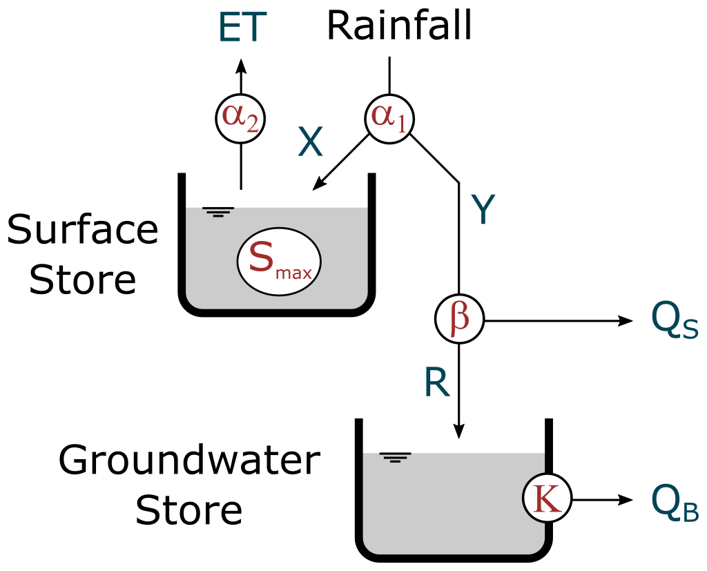
The WAPABA model is a conceptual monthly rainfall–runoff model introduced by Wang et al. (2011). The model is an evolution of the Budyko framework proposed by Zhang et al. (2008) where water fluxes are partitioned using parameterised curves. The model uses two inputs, mean monthly rainfall and potential evapotranspiration, and operates in five stages. First, input rainfall is split between effective rainfall that will eventually leave the catchment and catchment consumption that replenishes soil moisture and evaporates. Second, catchment consumption is portioned between soil moisture replenishment and actual evapotranspiration. Third, effective rainfall is partitioned between surface water (fast) and groundwater (slow) stores. Fourth, the groundwater store is drained to provide a baseflow contribution. Fifth, the surface water and baseflow are added to obtain the final simulated runoff for the month. The model has five parameters described in Table 2 which interact as depicted in Fig. 2.

Table 2 WAPABA model parameters.

Figure 2 WAPABA conceptual model schematic.

A separate WAPABA model is run for each study catchment. The WAPABA models were trained (calibrated) and tested (validated) over the same periods as the LSTMs: 1950 to 1995 inclusive for training and 1996 to June 2020 for testing. The model was calibrated with a warm-up period of 2 years to avoid possible bias associated with initial values. WAPABA parameters were optimised over the training period using the “shuffle complex evolution” algorithm (Duan et al., 1993) with the Swift software package (Perraud et al., 2015). The objective function used for the WAPABA models is the same as the one used for LSTM, i.e. the mean absolute error (MAE) on the square root of runoff (see Eq. 4).

2.3 Performance evaluation

Predictions from the conceptual (WAPABA) and machine learning (LSTM) models for all catchments are compared to observed runoff, assessing each model's predictive capabilities on the set of catchments. Runoff prediction performance is reported here using the following metrics.

The Nash–Sutcliffe efficiency (NSE; Nash and Sutcliffe, 1970) is the most often used performance metric in hydrology. It can be considered a normalised form of mean squared error (MSE) and is defined as

$$\begin{array}{}\text{(5)}& \text{NSE}=\mathrm{1}-{\displaystyle \frac{{\sum }_t(Q_{\text{obs}}^t-Q_{\text{mod}}^t{)}^{\mathrm{2}}}{{\sum }_t(Q_{\text{obs}}^t-{\mathit{\mu }}_{\text{obs}}{)}^{\mathrm{2}}}}=\mathrm{1}-{\displaystyle \frac{E}{V}},\end{array}$$

where $Q_{\text{obs}}^t$ and $Q_{\text{mod}}^t$ are the observed and modelled discharges for month t, respectively, and μ_obs is the average observed discharge over the training or testing period. The ratio of the sum of squared errors, $E={\sum }_t(Q_{\text{obs}}^t-Q_{\text{mod}}^t{)}^{\mathrm{2}}$, to the variance, $V={\sum }_t(Q_{\text{obs}}^t-{\mathit{\mu }}_{\text{obs}}{)}^{\mathrm{2}}$, is subtracted from a maximum score of 1. An NSE closer to 1 indicates better predictive capability of the model, and an NSE less than 0 indicates the model mean squared error is larger than the observation variance.

The NSE metric alone cannot provide an accurate description of model performance due to its focus on the high-flow regime (Schaefli and Gupta, 2007). The reciprocal NSE focuses the error metric on low flows (Pushpalatha et al., 2012) by comparing the reciprocals of the observed and modelled flows. It is calculated as

$$\begin{array}{}\text{(6)}& \text{RecipNSE}=\mathrm{1}-{\displaystyle \frac{{\sum }_t{\left({\displaystyle \frac{\mathrm{1}}{(Q_{\text{obs}}^t+\mathrm{1})}}-{\displaystyle \frac{\mathrm{1}}{(Q_{\text{mod}}^t+\mathrm{1})}}\right)}^{\mathrm{2}}}{{\sum }_t{\left({\displaystyle \frac{\mathrm{1}}{(Q_{\text{obs}}^t+\mathrm{1})}}-{\displaystyle \frac{\mathrm{1}}{({\mathit{\mu }}_{\text{obs}}+\mathrm{1})}}\right)}^{\mathrm{2}}}}.\end{array}$$

The Kling–Gupta efficiency (KGE; Gupta et al., 2009) provides an alternative to metrics based on sum of squared error, such as the two previous ones, by equally weighting measures of bias of the mean, variability, and correlation into a single metric as follows:

$$\begin{array}{}\text{(7)}& \text{KGE}=\mathrm{1}-\sqrt{{\left(\mathrm{1}-{\displaystyle \frac{{\mathit{\mu }}_{\text{sim}}}{{\mathit{\mu }}_{\text{obs}}}}\right)}^{\mathrm{2}}+{\left(\mathrm{1}-{\displaystyle \frac{{\mathit{\sigma }}_{\text{sim}}}{{\mathit{\sigma }}_{\text{obs}}}}\right)}^{\mathrm{2}}+(\mathrm{1}-\mathit{\rho }{)}^{\mathrm{2}}},\end{array}$$

where μ_X and σ_X are the mean and the standard deviation, respectively, and ρ is the Pearson correlation coefficient between the simulated and observed data.

Finally, “Bias” is a measure of consistent under-forecasting or over-forecasting of the mean, defined as

$$\begin{array}{}\text{(8)}& \text{Bias}={\displaystyle \frac{{\mathit{\mu }}_{\text{sim}}-{\mathit{\mu }}_{\text{obs}}}{{\mathit{\mu }}_{\text{obs}}}}.\end{array}$$

Comparison of performance metrics between catchments using normalised indexes

When comparing metrics across model types and catchments, a normalised difference in NSE values is used. The NSE metric can reach into large negative values in dry catchments when the variance of the observations is very small compared to the model errors (Mathevet et al., 2006), as can be seen from Eq. (5). Differences between large negative values of NSE have a much smaller implication than the same absolute difference between values of NSE closer to 1. To allow for a comparison between the WAPABA and LSTMs at catchments of various aridities, the normalised difference in NSE is calculated following Lerat et al. (2012):

$$\begin{array}{}\text{(9)}& \begin{array}{rl}{\text{Diff\_NSE}}_{\text{norm}}& ={\displaystyle \frac{{\text{NSE}}_{\mathrm{2}}-{\text{NSE}}_{\mathrm{1}}}{(\mathrm{1}-{\text{NSE}}_{\mathrm{1}})+(\mathrm{1}-{\text{NSE}}_{\mathrm{2}})}}\\ & ={\displaystyle \frac{{\text{NSE}}_{\mathrm{2}}-{\text{NSE}}_{\mathrm{1}}}{\mathrm{2}-({\text{NSE}}_{\mathrm{1}}+{\text{NSE}}_{\mathrm{2}})}},\end{array}\end{array}$$

where NSE₁ and NSE₂ are the NSE values corresponding to the two models to be compared. Substituting in $\text{NSE}=\mathrm{1}-\frac{E}{V}$ from Eq. (5) into Eq. (9), the normalised difference in NSE can be seen to represent a percentage difference in the sum of squared errors between the two models being compared:

$$\begin{array}{}\text{(10)}& {\text{Diff\_NSE}}_{\text{norm}}={\displaystyle \frac{{\text{NSE}}_{\mathrm{2}}-{\text{NSE}}_{\mathrm{1}}}{\mathrm{2}-({\text{NSE}}_{\mathrm{1}}+{\text{NSE}}_{\mathrm{2}})}}={\displaystyle \frac{E_{\mathrm{1}}-E_{\mathrm{2}}}{E_{\mathrm{1}}+E_{\mathrm{2}}}}.\end{array}$$

A similar formula is applied to reciprocal NSE and KGE. The normalised difference between the bias for two models is calculated as

$$\begin{array}{}\text{(11)}& {\text{Diff\_Bias}}_{\text{norm}}={\displaystyle \frac{\left|{\text{Bias}}_{\mathrm{1}}\right|-\left|{\text{Bias}}_{\mathrm{2}}\right|}{\left|{\text{Bias}}_{\mathrm{1}}\right|+\left|{\text{Bias}}_{\mathrm{2}}\right|}}.\end{array}$$

To simplify the comparison of model results across the large number of catchments, model performances at each catchment are classified as similar if the normalised difference between WAPABA and LSTM metrics lies within ±0.05 at that catchment, following Lerat et al. (2020). Therefore in this paper, a “similar” NSE denotes that the sum of squared errors of the WAPABA and LSTMs at an individual catchment differ by no more than 5 %. For differences greater than this, the catchments are classified by the model type producing the higher metric. The selection of the threshold of 0.05 was based on the recommendations of Lerat et al. (2020) and the authors' experience relative to the use of the NSE, KGE, and Bias metrics.

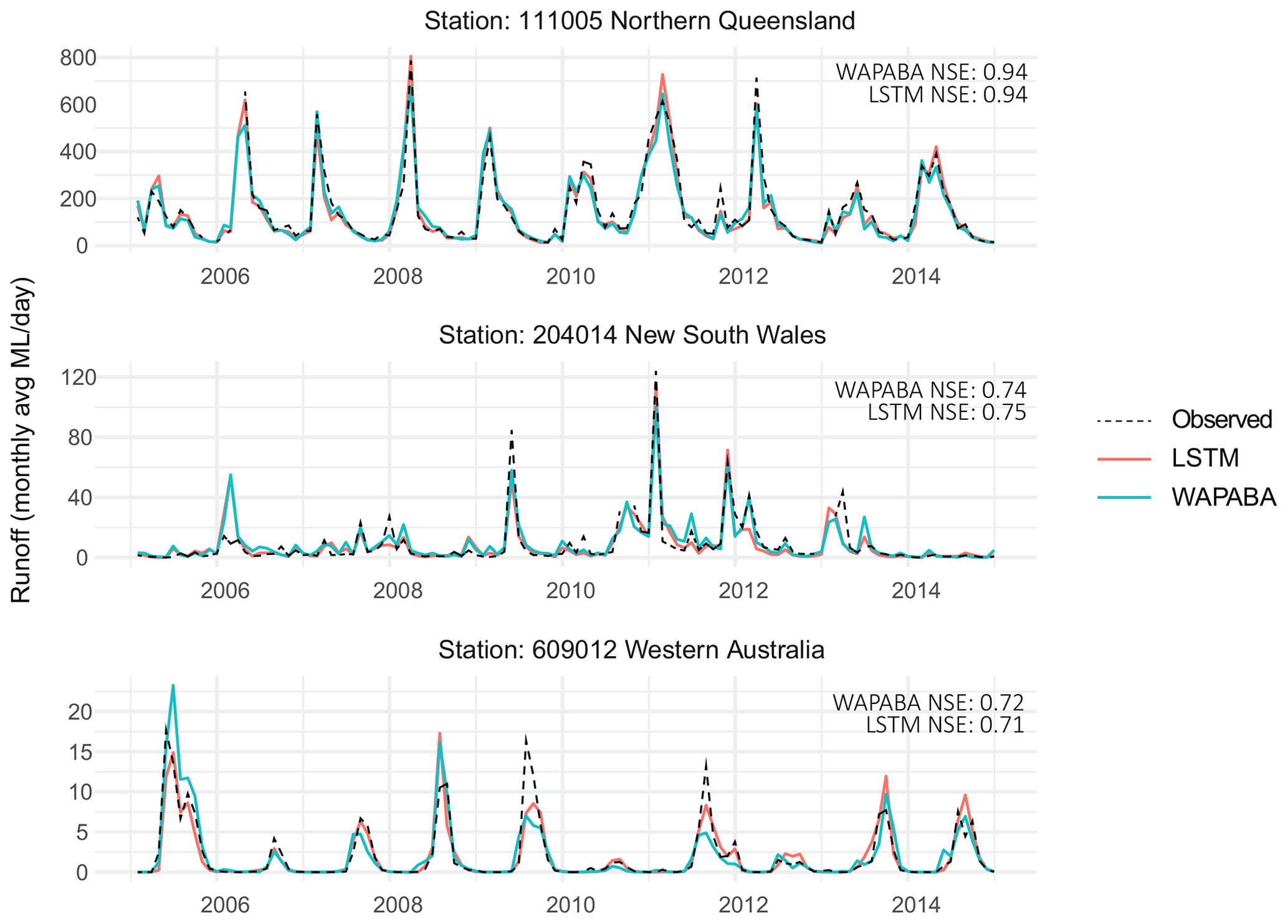
Figure 3 Observed data (black dashed line) and predicted runoff (by WAPABA and LSTMs) over the testing period for the Mulgrave River at The Fisheries (111005), Mann River at Mitchell (204014), and the Blackwood River at Winnejup (609012). Catchment locations are shown in Fig. 1.

3 Results

For each of the study catchments, a WAPABA model and an LSTM model have been trained using monthly data over the training period, and the prediction performance of the models are evaluated here on monthly data from the testing period (data unseen by the model during training) using the metrics described above. A general comparison of WAPABA and LSTM prediction performance is first made over all catchments with a continental-scale analysis of the performance metrics to determine

1. the proportion of overall catchments for which the WAPABA or the LSTMs produced better predictions and

2. differences at individual catchments in WAPABA versus LSTM prediction performance.

A comparison of model performance is then made in relation to various catchment and time series characteristics (e.g. catchment size, flow level, record length) to determine if an association exists between these properties and the relative performance of the conceptual and machine learning models.

3.1 Example prediction results

As a sample of the modelling output, Fig. 3 shows the WAPABA and LSTM runoff predictions along with the corresponding observed runoff for the three stations highlighted in Fig. 1 (over the testing period). These hydrographs are representative of a wet catchment in Northern Queensland (Mulgrave River at The Fisheries, 111005), a temperate catchment in New South Wales (Mann River at Mitchell, 204014), and a dry intermittent catchment in Western Australia (Blackwood River at Winnejup, 609012). NSE values of each of the predictions are noted. The WAPABA and LSTM predictions both match the observed data reasonably well in the three catchments. The performance of the models, in particular for the Blackwood River at Winnejup is remarkable because of the difficulty in modelling dry intermittent catchments (Wang et al., 2020). The next sections provide a more detailed assessment of the performance over all catchments using quantitative metrics.

3.2 Large-sample performance summary

The general runoff prediction performance of WAPABA and LSTMs on a continent-wide basis is summarised in Fig. 4. From the models run for each catchment, metrics are determined on the training portion (calibration) and testing portion (validation) separately and gathered here in boxplots. Median and quartiles of NSE, reciprocal NSE, KGE, and Bias over all catchments are shown for each model type, with each data point representing an individual catchment. All data are shown on the top panel, and due to a few large (negative) outliers the same figure is shown with a restricted y axis for visualisation purposes on the lower panel. Higher values of the first three metrics (NSE, reciprocal NSE, and KGE) indicate a better match of predicted runoff with observed runoff, whereas lower values of Bias indicate better prediction results.

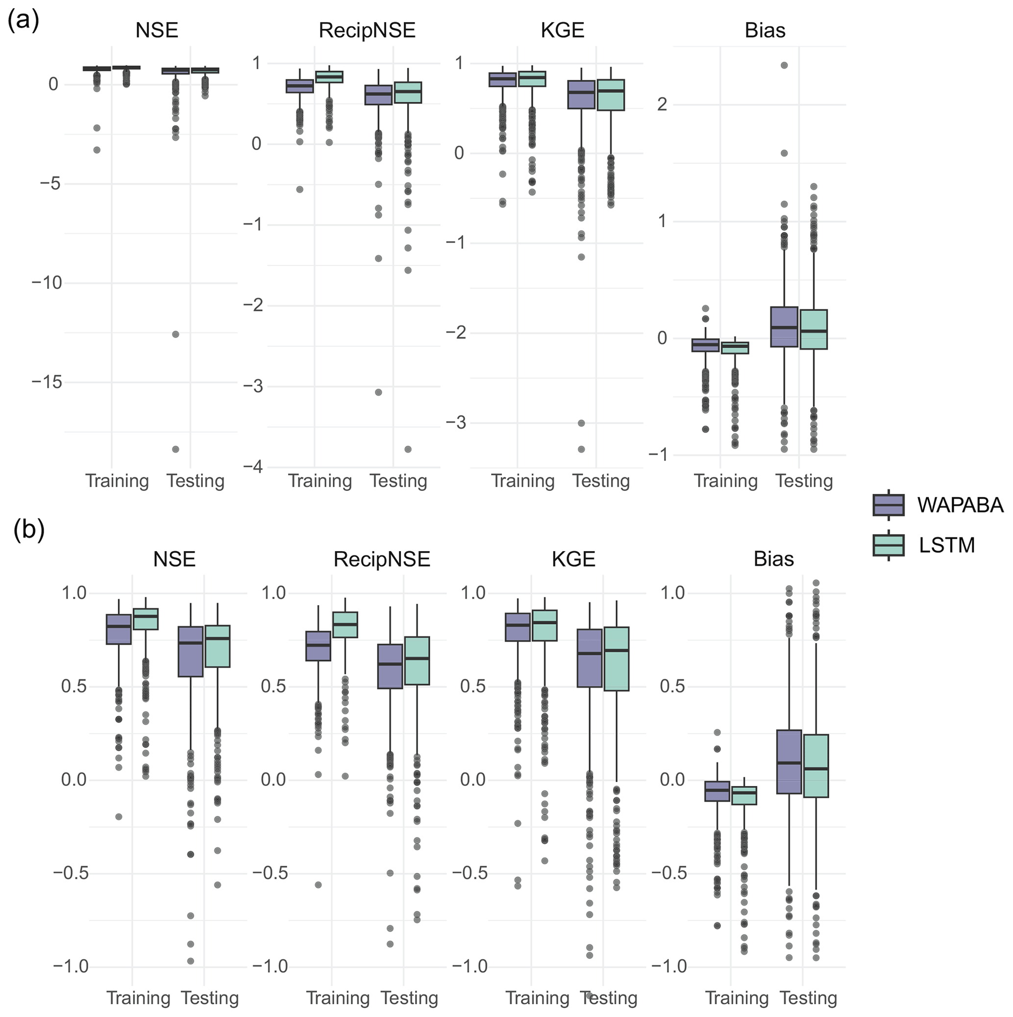
Figure 4 Performance metrics summary for the set of 496 catchments (zoomed-in view in panel b, excluding outliers $<-\mathrm{1}$). Median values of LSTM performance metrics are slightly higher than WAPABA for NSE, reciprocal NSE, and KGE (higher indicates better performance) and slightly lower for Bias (lower Bias is preferable). For all four metrics on both models, the longer testing boxes indicate more spread in performance results when predicting on new data.

Figure 4 shows that across the set of study catchments the median values of NSE, reciprocal NSE, and KGE are slightly higher for LSTM than for WAPABA during both the training and testing phases. Bias has a slightly lower median for the LSTM. As expected, both model types perform better during the training phase than the testing phase for all metrics. The difference between WAPABA and LSTM performance is relatively large during the training period but similar during testing, indicating perhaps a higher tendency towards overfitting by the machine learning models than traditional modellers would be expecting. The interquartile ranges increase from training to testing (longer boxes during testing), indicating a greater spread of performance results when the models are run on data not seen during the training phase. Over all catchments, the median NSE is 0.74 with the WAPABA models and 0.76 with the LSTMs (on testing data). See Table 3 for median values of these metrics.

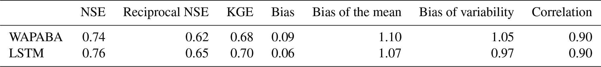
Table 3 Median values of metrics over the set of catchments (n=496).

Aggregated performance metrics may mask performance variability within certain aspects of the time series (Mathevet et al., 2020). The KGE has the benefit of being easily decomposed into three components for further error analysis: bias of the mean (ratio of mean of simulations to mean of observations), bias of variability (ratio of standard deviation of simulations to standard deviation of the observations), and correlation (matching of the timing and shape of the time series to the observations).

In Fig. 5 and Table 3, model performance is assessed with respect to each component of the KGE metric. Boxplots of the decomposed KGE components are shown by model type and training/testing period. During testing, the medians of bias of the mean and standard deviation are above zero for WAPABA and greater for WAPABA than LSTM. This indicates that mean streamflow and streamflow variability tend to be overestimated more by the WAPABA models compared to the LSTMs. The LSTM median bias of variability is below zero; therefore, streamflow variability is more prone to underestimation. For bias of the mean and standard deviation, the depth of the boxplots increases from training to testing, indicating the bias values from individual catchments are more diverse during the testing period.

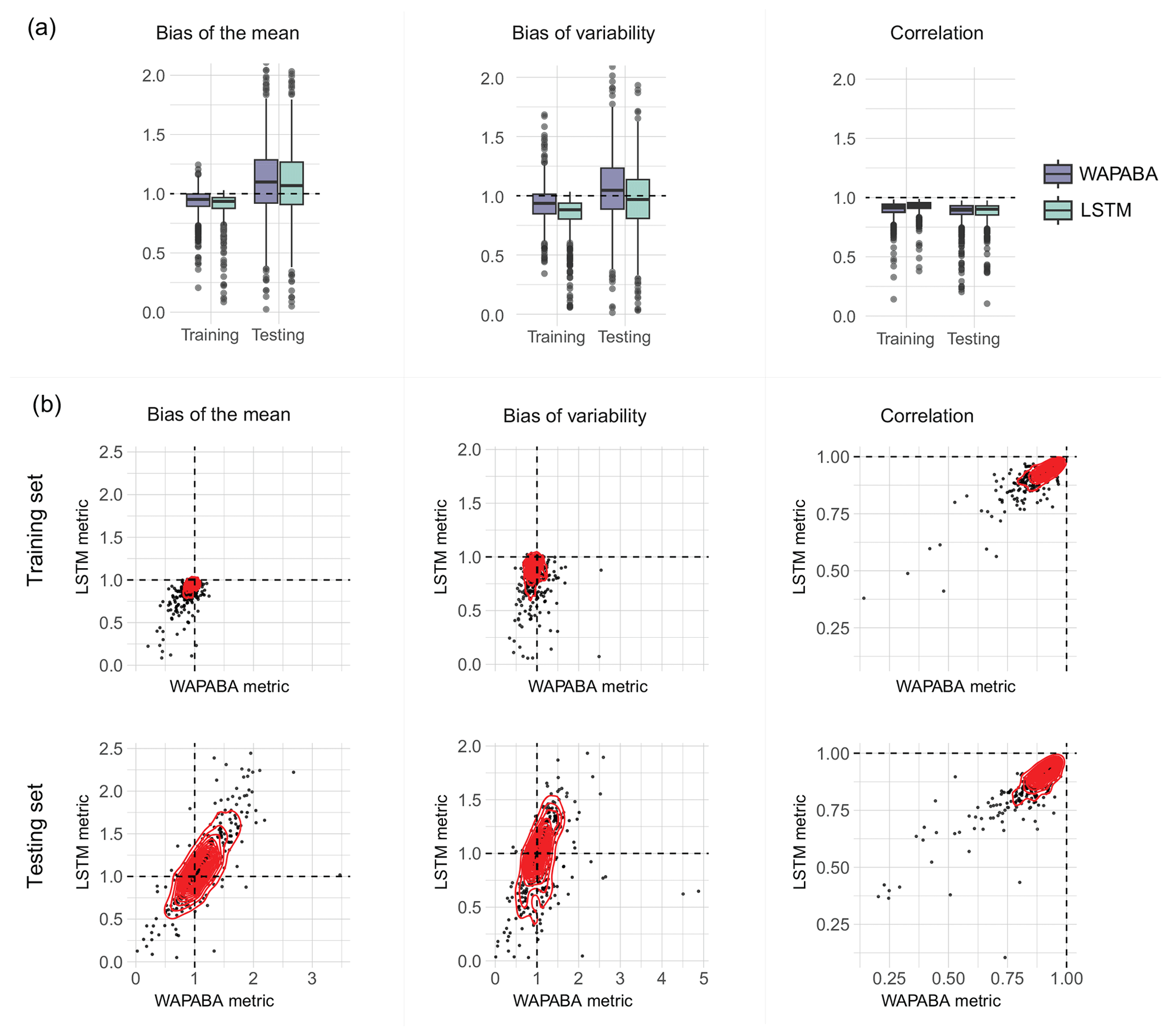
Figure 5 KGE decomposition into three components: bias of the mean, bias of variability, and correlation. Each dot represents an individual catchment (large outliers have been omitted for visualisation purposes). In panel (a), boxplots show the median and interquartile range of each category; in panel (b) scatterplots compare the distributions. The mean flow and variability (left and middle columns) tend to be underestimated during training and both underestimated and overestimated during testing by both model types. The correlation (right column) remains similar during training and testing.

The scatterplots in the lower part of Fig. 5 compare the KGE components at individual catchments for the WAPABA and LSTMs (each dot represents a catchment), separately for training and testing portions of the data. Most values of bias of the mean (left column) are between 0 and 1 during training (underestimating) yet during testing values extend beyond 2, indicating that the mean flow in many catchments is overestimated by both model types on the testing data. The observable correlation in testing period bias of the mean between WAPABA and LSTM indicates that this error is not specific to model type. The correlation between simulations and observed data is similar for both model types and remains relatively constant between training and testing periods (right column).

3.3 Performance differences at individual catchments

The differences between WAPABA and LSTM performance at each catchment (e.g. ${\text{NSE}}_i={\text{NSE}}_{i,\text{WAPABA}}-{\text{NSE}}_{i,\text{LSTM}}$ for catchment i) are summarised in Fig. 6. Values above zero indicate higher metrics obtained by WAPABA, and values below zero indicate higher metrics obtained by the LSTM model at a specific catchment.

Figure 6 Difference in the metrics (WAPABA−LSTM) for each catchment. A positive value indicates WAPABA has a higher metric for that catchment, and a negative value indicates LSTM has a higher metric. The median difference in each metric lies close to zero for the testing portion of the dataset, signifying overall similarity in catchment-specific metrics between model types. Large negative outliers have been excluded from this figure for visualisation purposes but are provided in Fig. A1 in Appendix A.

The boxplots indicate that median differences in WAPABA and LSTM prediction performance at each catchment (measured by NSE, reciprocal NSE, KGE, and Bias on the testing data) are very close to zero. However, there are outliers (black dots) representing large performance differences between WAPABA and LSTMs, both positive and negative. These indicate that each model provides advantages for predicting runoff in certain catchments. In this figure the boxplots are restricted to the range $[-\mathrm{1},\mathrm{1}]$ for visualisation purposes. A version of this figure including the large outliers is provided in Fig. A1 of Appendix A.

This dataset represents a range of catchments across Australia, with some being characterised by highly arid conditions. To enable comparisons between these diverse catchments, the impact of large negative NSE values which can occur at very dry catchments is minimised by calculating the normalised differences in NSE between the WAPABA and LSTM predictions at each catchment, as per Eq. (9). The normalised differences fall into the range $[-\mathrm{1},\mathrm{1}]$, facilitating comparison. This distribution is shown in Fig. 7 for the 496 catchments. The portion of the distribution lying to the right of the vertical dashed line corresponds to catchments with better prediction by WAPABA and catchments to the left have better prediction by LSTM. The x axis corresponds to percentage differences between the sum of squared errors of the two model types (i.e. −0.5 indicates a 50 % performance gain by LSTM, and 0.5 indicates a 50 % performance gain by WAPABA).

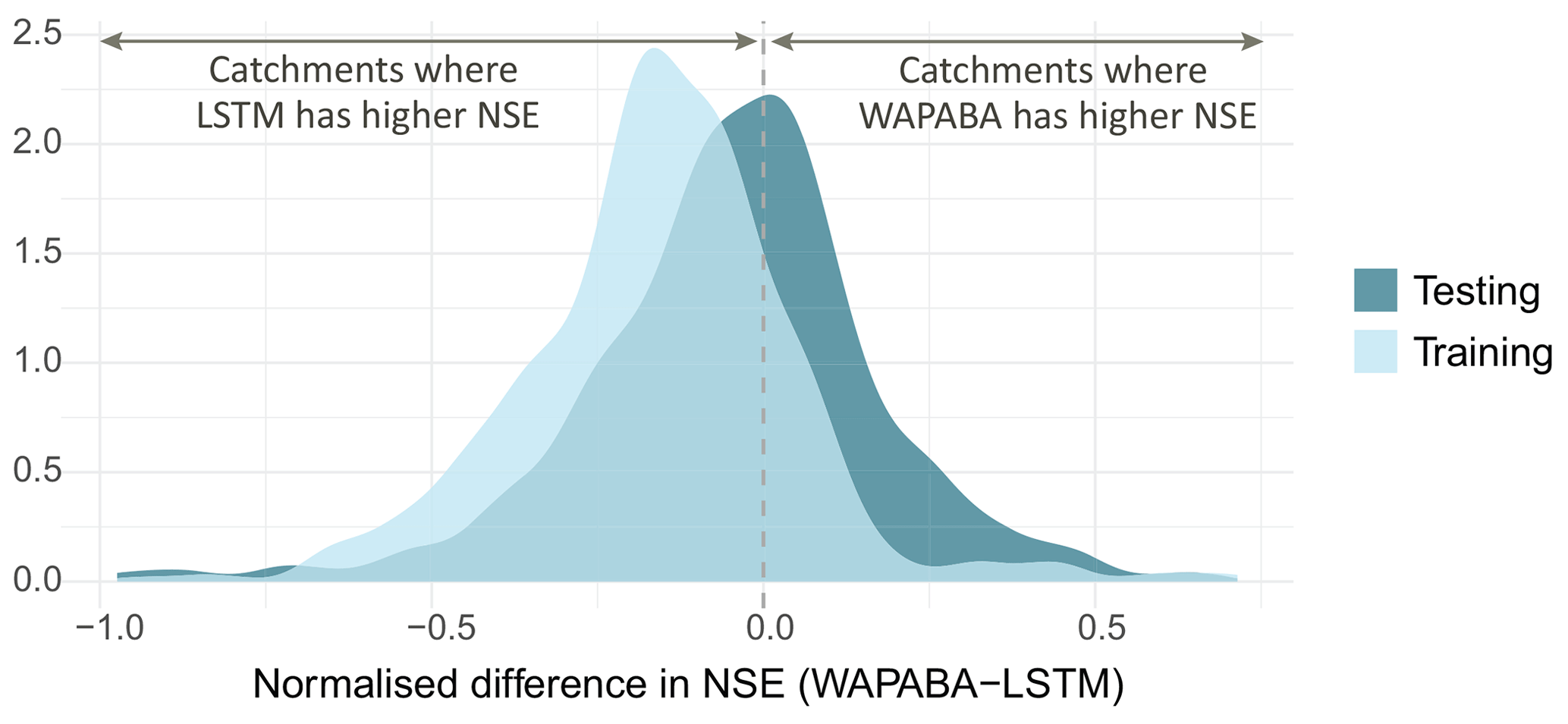
Figure 7 Distribution of normalised differences between WAPABA and LSTM prediction performance at individual catchments (measured by NSE). The values on the x axis represent percentage$/$100 difference in sum of squared errors between WAPABA and LSTM at the same catchment (i.e. 0.5→50 % difference in sum of squared errors). The catchments under the curve on the right of the dashed line have better predictions by the WAPABA model and on the left by the LSTM model.

In Fig. 7, it can be seen that during the training period the majority of catchments are to the left of the line, indicating better prediction by LSTM, and in the testing period there is a more even split. The median normalised difference in NSE across the 496 catchments over the training period is −0.15 (mean −0.16) and −0.04 (mean −0.05) during the testing period. This equates to a median 15 % performance advantage by LSTM versus WAPABA during training and 4 % during testing based on sum of squared errors.

This figure suggests that in general there is little overall advantage of either the WAPABA or LSTMs when predicting on unseen data across the whole sample of catchments. However, the width of the distribution indicates that both the WAPABA and LSTMs have advantages at certain individual catchments, which will be explored in the next section.

Figure 8 quantifies the proportion of catchments with similar or better prediction performance by either WAPABA or LSTM (on the testing data). “Similarity” is defined here as an absolute normalised difference in NSE of less than 0.05 between WAPABA and LSTM predictions, meaning the sum of squared errors of the WAPABA and LSTMs at an individual catchment differ by no more than 5 %.

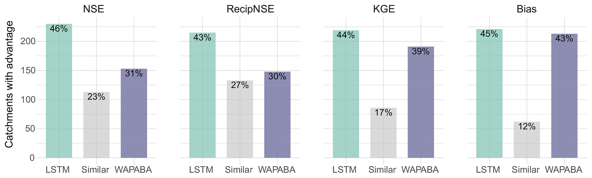
Figure 8 Percentage of catchments with similar or better performance metrics on the testing portion of the data (note lower values of Bias are better, for all other metrics higher is preferable). For catchments in the “similar” category, the sum of squared errors of the WAPABA and LSTM predictions differ by less than 5 %. The LSTM model produces predictions with similar or higher NSE values compared to the WAPABA predictions for 69 % of the catchments.

The LSTMs produce similar or higher NSE values for 69 % of the catchments when tested on data not seen during the training process (and 89 % of the catchments during training, not shown). It can also be seen that 70 % of catchments have similar or higher reciprocal NSE (focusing on low flow predictions) with the LSTM, 61 % have similar or higher KGE with the LSTM (higher being preferable), and 57 % have similar or lower Bias (lower being preferable) with the LSTM model compared to WAPABA on the same catchment.

3.4 Prediction performance comparison by catchment or time series characteristics

In this section, it is investigated if the abilities of WAPABA and LSTM to accurately predict runoff at individual catchments vary based on attributes such as catchment area, flow level, and length of historical record.

3.4.1 Catchment size

Figure 9 shows the association of prediction performance with catchment area. The left panel shows the catchment area compared to the normalised difference in NSE between LSTM and WAPABA prediction performance for each catchment. Data points are coloured according to the model that produced the better prediction for that catchment. This figure indicates the largest performance gains of LSTM versus WAPABA occurred in large catchments (points furthest to the left are found in the upper portion of the plot). Splitting the catchments into quintiles by area, the results can be analysed for the largest 20 % of catchments. Of these catchments, over three-quarters (78 %) had similar or better runoff predictions with the LSTM (with similarity defined as less than 5 % difference in sum of squared errors compared to WAPABA predictions). In this top quintile of catchments by area, those with higher NSE values from the LSTM show a greater average advantage (average 24 % lower sum of squared errors, maximum 97 % lower), than those with better WAPABA predictions (average 15 % lower sum of squared errors, maximum 65 % lower).

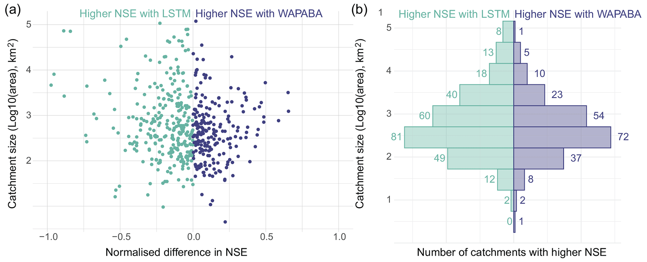
Figure 9 Model performance by catchment size. (a) Each data point represents the normalised difference in prediction performance at an individual catchment, arranged by catchment size. The spread of data points in the top left quadrant indicates that in large catchments the performance gain of LSTM over WAPABA can exceed 90 % in terms of sum of squared errors. (b) Count of catchments in each size category that have better performance with each model.

The mirrored histogram in the right panel of Fig. 8 shows catchments stratified into bins by area (log base 10), coloured and counted by the model type that produced the better runoff prediction at each catchment. The LSTMs produced higher NSEs for a greater number of catchments than the WAPABA models in all of the bins, except the lowest bin (where n=1).

3.4.2 Flow level

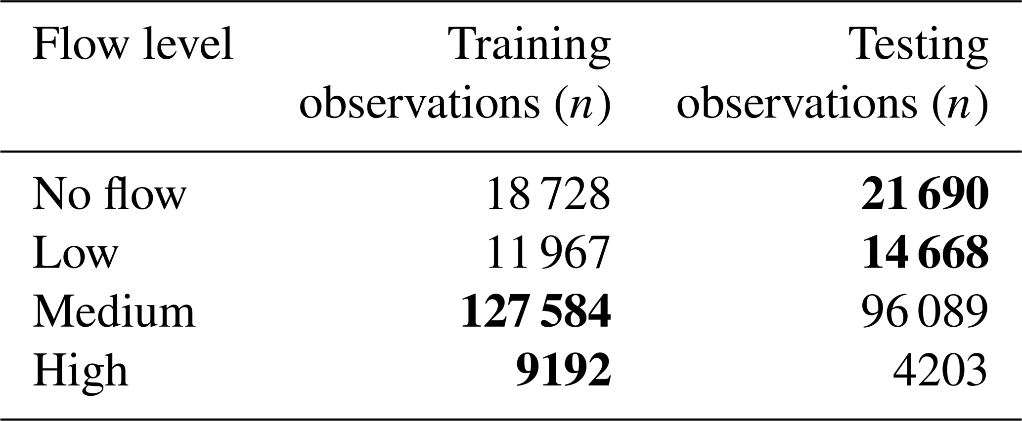
Model performance is compared for high-, medium-, and low-flow portions of the time series. For each station, each observation is categorised based on its flow level. High flows are defined here as the top 5 % of flow values and low flows as the lower 10 % of flows at each station (calculated excluding zeros) over all observed data during the study period. The training and testing portions of the time series over all the catchments have different distributions of flow levels, as listed in Table 4. During the testing portion of the study period, conditions are dryer with more no-flow and low-flow observations and fewer medium- and high-flow observations than during training.

Table 4 Distribution of flow levels during training and testing periods. Bold entries indicate the maximum in each flow level.

For comparison purposes in this section, the raw observed and modelled flow data are standardised by station based on the mean and standard deviation of all observations at that station during the study period. The observed mean is subtracted from each value before dividing by the standard deviation of the observations, allowing for basins with a range of flow volumes to be compared.

Figure 10 shows that when NSE is calculated separately for the low-, medium- and high-flow measurements at each catchment, both model types have similar NSE distributions. Medium flows are better predicted (NSE peak closer to 1) than high flows, and low flows appear to be poorly represented by both WAPABA and the LSTM.

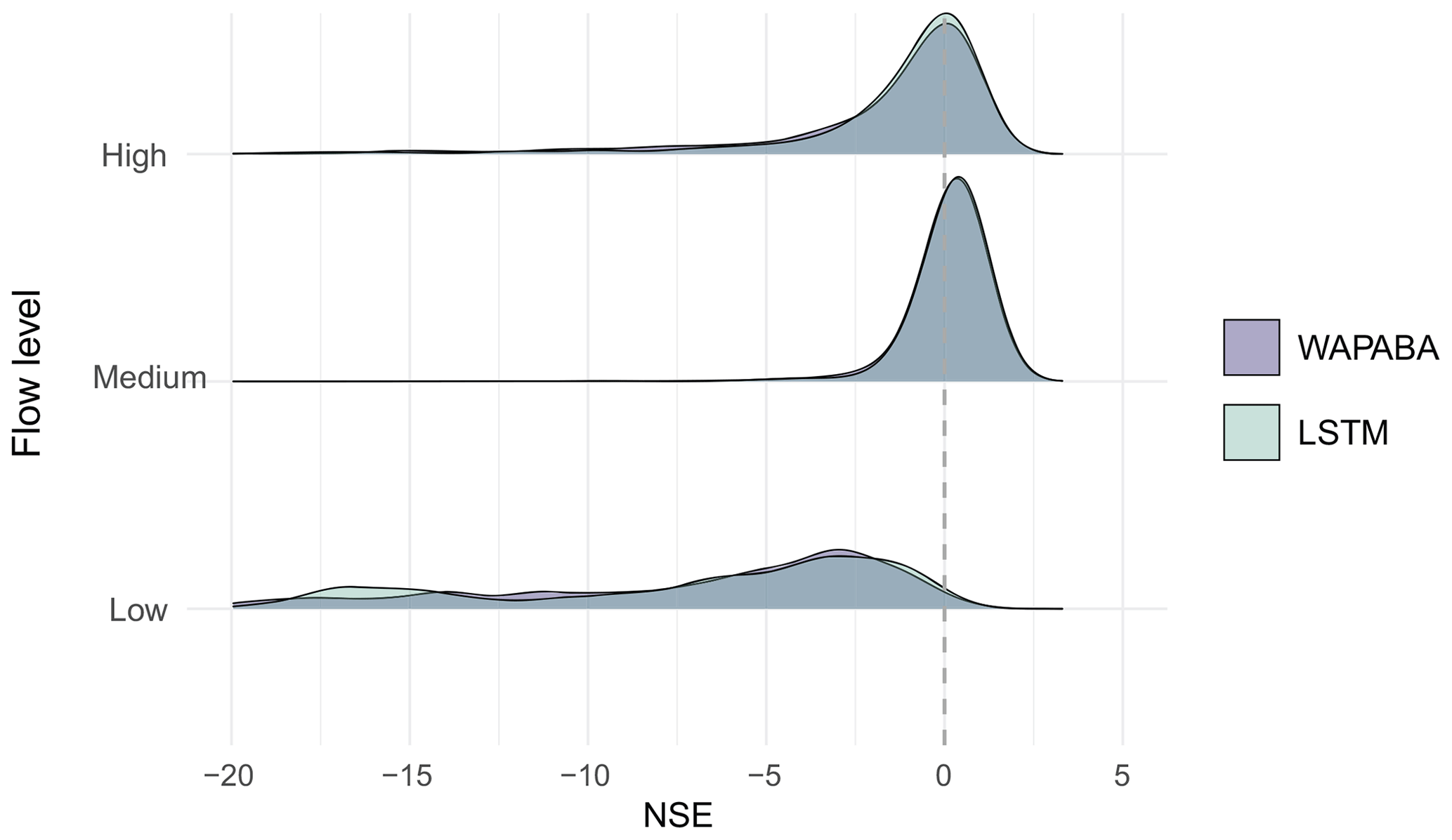
Figure 10 NSE distributions calculated separately by flow level over all catchments. Both model types have similar distributions of NSE by flow. Medium flows are best represented, followed by high and then low flows.

Figure 11 compares the standardised modelled flow to the standardised observations for all testing observations at all stations. Kernel density contours split the data into 10 density regions on each plot, and a 1:1 line is added to aid interpretation. The lower panel focuses on the regions of highest density for each subset of flows. Note that the standardisation procedure used in this section leads to standardised “no-flow” data points that do not fall exactly on zero in the plot even though the raw flow values at these points are zero. For no flows and low flows (left two panels), the densest portions of the observation/prediction clouds are closely aligned along the 1:1 line, indicating similar predictions obtained with both models. The magnitude of the outliers (beyond the outermost contour) is greatest above the 1:1 line indicating that prediction errors for no flows and low flows are dominated by overestimations. For medium-flow levels, the contours again follow the 1:1 line. The contours tend to expand upwards as flow size increases, indicating a tendency towards more overestimation with higher flows. The shape of the contours is similar for both models. On the upper panel, it can be seen that the edges of the data cloud expand upwards and outwards as the flows increase. The medium-flow prediction errors with largest magnitude tend to be overestimations, with the WAPABA models producing greater overestimations than the LSTMs on the higher flows (still in this medium-flow subset). For high flows (on the far right panel), the majority tend to be underestimated by both LSTM and WAPABA (central density located below the 1:1 line), though there is a difference in the outliers – most of the larger errors in LSTM high-flow predictions are underestimations, whereas the high-magnitude WAPABA errors are both overestimations and underestimations of high flows.

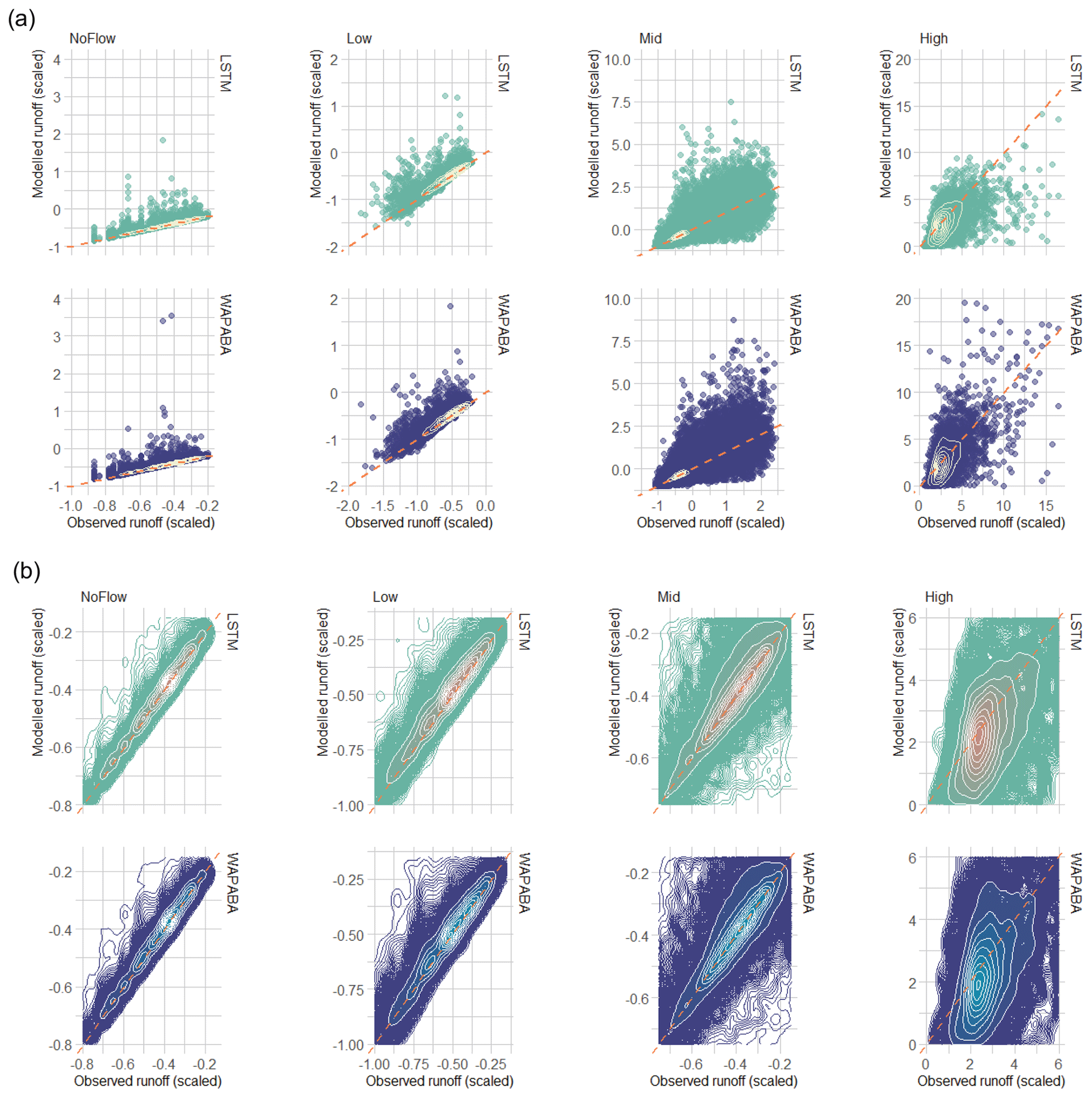
Figure 11 Prediction performance related to flow level. (a) Observed vs. modelled flow pairs (normalised data) at all stations, separated into no-flow, low, medium and high flows (testing data only). The densest portion of the data cloud is identified with density contours. Note that the data have been standardised based on observed mean and standard deviation leading to non-zero values in the “no-flow” category. (b) Comparison of density distributions of the data, zoomed in on the kernel density contours. In general, the largest errors on medium flows tend to be overestimations (by both models) and on high flows tend to be underestimations (by both models) or overestimations (by WAPABA).

3.4.3 Poorly predicted catchments

Figure 12 compares the NSEs for WAPABA and LSTM runoff predictions by catchment. Each dot represents an individual catchment, coloured according to the model with higher NSE at that catchment. The top left quadrant contains catchments where NSE_WAPABA<0 and NSE_LSTM>0 (n=19), and the lower right quadrant contains catchments where NSE_LSTM<0 and NSE_WAPABA>0 (n=5).

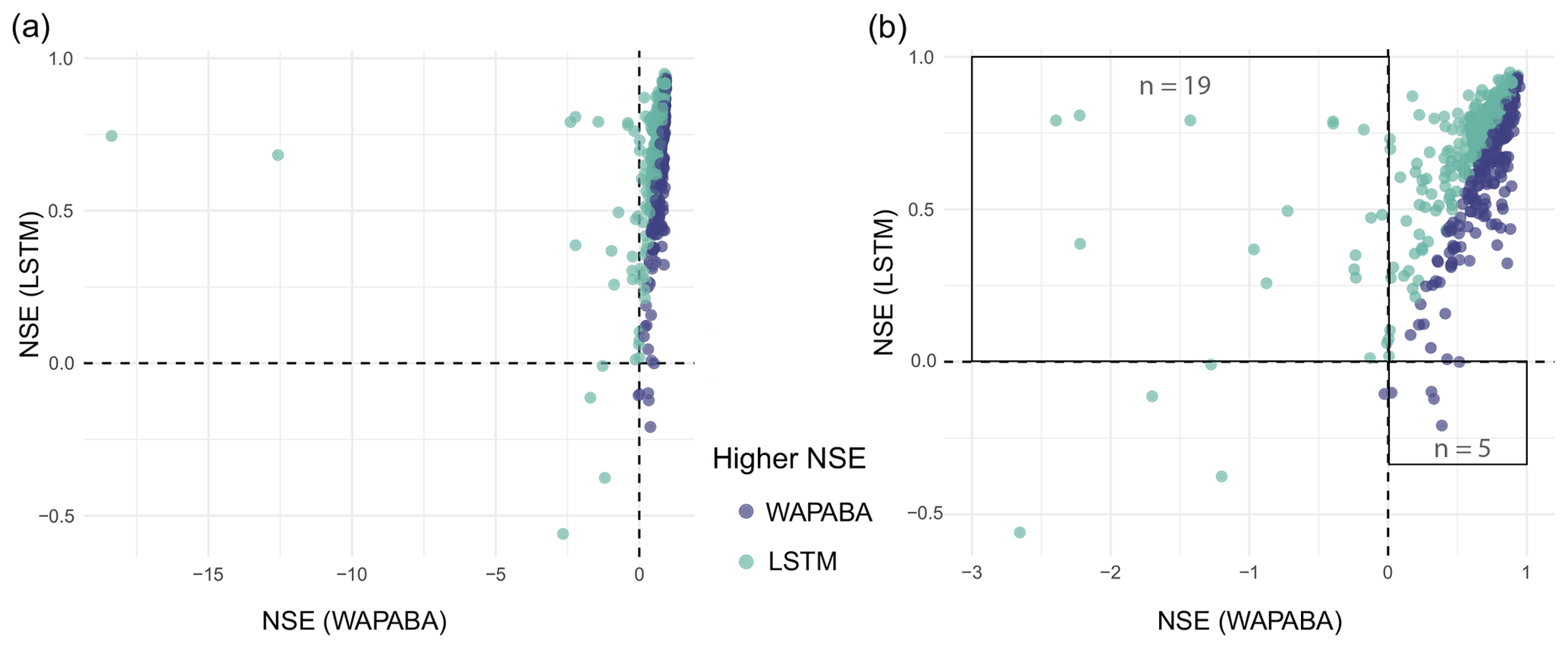
Figure 12 (a) Comparison of NSEs on testing data – each data point represents the WAPABA and LSTM values of NSE for a single catchment, coloured by the model which provides the best prediction at that catchment. In panel (b), two far-left outliers have been removed to enable better viewing of the other data points. Catchments in the upper left quadrant are those in which runoff is poorly predicted by WAPABA (NSE<0) and better predictions (NSE>0) are obtained with LSTM. The lower right quadrant correspondingly shows catchments in which the NSE values from LSTM are below 0 and WAPABA has better predictions (NSE>0).

WAPABA and LSTM predictions at each catchment are classified into poor (NSE<0), fair ($\mathrm{0}\le \text{NSE}\le \mathrm{0.5}$), or good (NSE>0.5) categories. In this set of catchments, the runoff at 5 catchments is poorly predicted (NSE<0) by both model types (lower left quadrant of Fig. 12). All other catchments are better represented by one model or the other, with either WAPABA or LSTM producing predictions with NSEs above 0.

For the 5 % (n=24) of overall catchments that are poorly represented by WAPABA (NSE<0), runoff predictions at 23 of these catchments (96 %) are improved with use of the LSTM. In fact, one-third (n=8) of these have good predictions by the LSTM (NSE>0.5). Conversely, for the 2 % of catchments (n=10) that are poorly represented by the LSTM, 60 % are improved with use of WAPABA, and one-tenth (n=1) have good predictions by WAPABA (in this catchment the LSTM prediction is on the border of poor and fair (NSE=0.001)). Figure 13 depicts the number of catchments poorly represented by each model and how these specific catchments are represented by the alternate model. For half of the catchments with poor LSTM predictions, WAPABA does poorly as well, whereas in 79 % of the catchments with poor WAPABA predictions fair or good predictions were obtained with the LSTM.

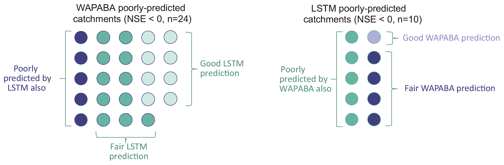
Figure 13 Number of catchments with poor runoff predictions by each model type. Colouring indicates the prediction results from the alternate model type. One-third of WAPABA poorly predicted catchments have good predictions with the LSTM. One-tenth of LSTM poorly predicted catchments have good predictions with WAPABA. Results are denoted as poor (NSE<0), fair ($\mathrm{0}\le \text{NSE}\le \mathrm{0.5}$), or good (NSE>0.5).

3.4.4 Generalising to changing conditions

The ability of a model to generalise outside of the conditions encountered during training is important, especially in the context of a changing climate. A model that is able to make predictions on unseen (testing) data to a comparable performance level as on the training data will provide confidence in making predictions into the future when external conditions are not expected to remain constant. In this dataset, it is known that conditions differ between the training and testing data, with wetter climate conditions during the training period and a dryer testing period.

It was found that 2 % (n=11) of WAPABA models struggled with generalising outside of the training period, with good (NSE>0.5) runoff predictions during training but very poor predictions ($\text{NSE}<-\mathrm{0.5}$) during the testing period. The testing predictions for all of these catchments were improved by use of the LSTM, and at four of these catchments good predictions (NSE>0.5) were obtained with the LSTMs. Conversely, one LSTM model produced good training runoff predictions and very poor testing predictions. This catchment was 1 of the 11 that also had poor generalisation (and very poor predictions) with WAPABA.

3.4.5 Historical record length and dataset size

The performance of each model type is compared to the length of historical records available at each station. Training data length has been categorised here as 14–25 years (38 % of stations), 25–35 years (40 %), and 35–47 years (23 %).

Figure 14 (top panel) shows prediction performance varying slightly with record length (for visualisation purposes, this figure is shown without large negative outliers – the figure including outliers is provided in Fig. A2 of Appendix A). Stations with medium record length tend to have slightly better predictions according to the four metrics than those with shorter records. The performance levels tend to even out as record lengths increase beyond 35 years, and there is even a slight decline in the WAPABA reciprocal NSE.

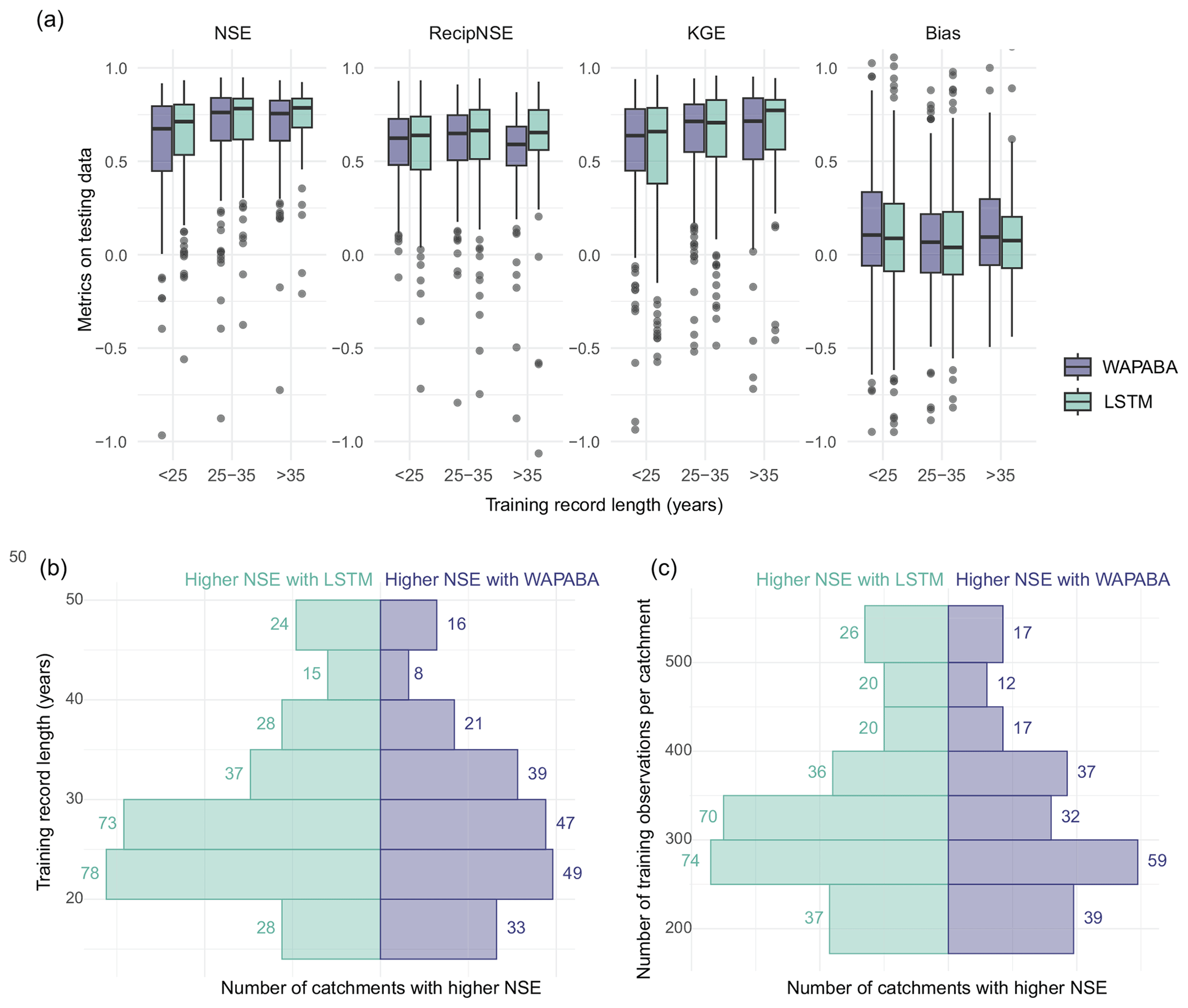
Figure 14 Effect of record length and training data size on prediction performance for each model type. (a) Medians of the NSE and KGE on testing data increase with record length for both WAPABA and LSTM predictions (large negative outliers have been excluded for visualisation purposes but are included in the corresponding figure in Appendix A). (b) Advantage of each model in 5-year increments of record length based on NSE values. (c) Advantage of each model based on number of training observations.

Considering catchments individually, the median normalised difference in NSE between WAPABA and LSTM predictions (on testing data) is just slightly below zero for all record lengths: −0.03 (<25 years of record), −0.04 (25–35 years), and −0.04 (>35 years). This indicates that, in each of the short, medium, and long record length categories, at least half of the individual catchments have higher NSEs with the LSTMs.

The mirrored histogram in the lower left panel of Fig. 14 quantifies the number of catchments within 5-year bins of record length in which runoff is better predicted by the LSTM or by the WAPABA. In six of the eight bins, the majority of catchments are better represented by the LSTM.

Comparing performance based on the number of years of record does not take into account the actual size of the datasets, since measurement frequency differs at each station. Catchments in this study have between 172 and 564 training data observations (425–846 including testing data). The lower right panel of Fig. 14 shows the number of catchments best modelled by the WAPABA or LSTM model (determined by higher NSE on the testing data) in relation to the number of training observations. Median NSE values of both the WAPABA and LSTM predictions increased with increasing number of training data points (not shown). Of particular note is that runoff at catchments with the smallest datasets (less than 250 training data points) were similarly well predicted by both LSTM (median NSE=0.67) and WAPABA (median NSE=0.66).

4 Discussion

When considered over the entire study set of catchments, machine learning models were found to match conceptual model performance for the majority of catchments. The median NSE of runoff predictions was 0.74 with the WAPABA models and 0.76 with the LSTMs, and the medians of other metrics were similarly aligned. At individual catchments, LSTM runoff prediction performance was similar to or exceeded WAPABA performance in 69 % of the catchments in this study (based on the NSE metric). The median differences in metrics (NSE, reciprocal NSE, KGE, and Bias) between the model types at individual catchments were close to zero, though the range of differences was wide in both directions, suggesting many catchments had noticeable prediction advantages with either the WAPABA or LSTMs.

Medium flows were similarly well represented by both model types, with less accurate predictions for high flows and worse again for low flows. Both WAPABA and LSTM models tend to overestimate low flows, while high flows are noticeably underestimated by LSTM and both overestimated and underestimated by WAPABA. Across all flow levels, the mean flow is prevalently overestimated during testing for both model types, though slightly more so by WAPABA (higher bias of the mean). This overestimation is expected as the testing period in this study is drier than the training period and it is common to have an overestimation of mean during dry periods (Vaze et al., 2010). Variability of streamflow tends towards overestimation by WAPABA and underestimation by LSTM.

Larger catchments were found to have the potential for greater prediction improvements with the LSTM. This finding supports the work of Fluet-Chouinard et al. (2022), who found that deep learning methods compete especially well with traditional models in larger non-regulated rivers where the influence of time lags is significant.

Though it is known that, in general, machine learning models benefit from large amounts of training data, it is often not possible to provide large hydrological datasets. In this comparison, shorter training record lengths were not found to affect one model type more than the other; the catchments with the smallest training datasets (less than 250 observations) did not show a distinct prediction advantage with either WAPABA or LSTM (median NSEs of 0.66 and 0.67 respectively).

In past studies, traditional models have been found to struggle to make accurate runoff predictions under shifting meteorologic data (Saft et al., 2016). Researchers have noted that deep learning models may have the potential to overcome this issue (Li et al., 2021; Wi and Steinschneider, 2022). In this study, the variation in differences in prediction performance at individual catchments is more evident during the testing portion than the training portion of the time series, implying that the WAPABA and LSTMs may each have advantages or drawbacks for generalising to unseen data on various catchments. It was found that in catchments where the WAPABA models provide good runoff predictions during training but struggle to make accurate predictions on new data, the LSTM provides improved predictions in all cases (i.e. for those with testing NSE<0 with WAPABA, all bar one had NSE>0 with the LSTM). In the opposite case, where the LSTM produced substantially poorer predictions on testing data than training data, these predictions were not outdone by WAPABA. This improvement by the LSTM in predicting beyond conditions experienced during training will become progressively important as climate change continues.

Aside from scientific considerations, another important advantage of developing rainfall–runoff models using a machine learning software framework is to easily share them among users and to benefit from software optimisation provided by well-established frameworks such as TensorFlow, Keras, or PyTorch. Better benchmark datasets and centralised repositories will be the key to advancement of machine learning in hydrology (Nearing et al., 2021; Shen et al., 2021). Initiatives are being made to grow reusable software for applying machine learning in hydrology and to benchmark these against other approaches (Abbas et al., 2022; Kratzert et al., 2022).

Metrics and models

Certain caveats are acknowledged regarding the metrics and models used here. It is possible that the use of individual metrics to compare predictions along the entire length of the time series may mask any variability in model performance that occurs in subperiods of the time series (Clark et al., 2021; Mathevet et al., 2020). These limitations were partially addressed by comparing high-, medium-, and low-flow periods separately, though there are many other subdivisions of the time series that have not been included in the scope of this study.

WAPABA is only one example of a conceptual rainfall–runoff model. There are others that could have been chosen for this analysis, though fewer are suitable for comparisons at a monthly time step than would be the case at the daily time step. Model comparisons in Wang et al. (2011), Bennett et al. (2017), and the subsequent body of work with WAPABA in Australia have established WAPABA as a reasonable benchmark against which to assess the machine learning model performance.

Though this study has focused on comparing the LSTM model to the WAPABA, readers may wonder if the more traditional feed-forward neural network (FFNN) may suffice in producing as good results. The FFNN has been used in hydrology for many years to model the relationship between climatic predictors and hydrological responses and many researchers are familiar with this basic neural network structure. However, the FFNN is a static network and does not consider the sequential nature of the input data. Though the 6 months of lagged predictor variables could be input as separate variables, this requires an increase in the complexity of the training space and is not likely to be the optimal choice for time series data as the cumulative impact of the predictor sequences may not be captured. Many studies have already considered the comparison of FFNNs to LSTMs for rainfall–runoff modelling and have determined the LSTM to provide superior runoff predictions (e.g. Rahimzad et al., 2021). As an experiment, the FFNN has been run on this set of 496 catchments and added to the comparison of overall model performance, shown in Fig. A3 of Appendix A. It can be seen that the FFNN leads to lower NSE, KGE, reciprocal NSE, bias of the mean, bias of variability, and correlation values, and it therefore provides less accurate estimations of runoff than both the WAPABA and the LSTM. For this reason, the FFNN has not been included in the bulk of this study.

Future research directions

Future work may entail an expansion of the architecture and complexity of the LSTMs used here to determine what advantages could be gained from the use of more sophisticated model setups. This may involve the development of hybrid models blending existing conceptual models with LSTMs, the production of a global LSTM incorporating all of the time series, or a type of transfer learning where a model trained on data from all catchments is fine-tuned on a catchment-by-catchment basis, as in Kratzert et al. (2019).

A simple LSTM has been used in this study, with a single layer and no catchment-specific hyperparameter tuning. Through appropriate tuning of the models' architecture and hyperparameters for each catchment, more accurate results could be expected. For example, it is known that the performance of data-driven runoff models is heavily dependent on the amount of lagged data that are used as input (Jin et al., 2022). In this study, a lag of 6 months has been used for all of the catchments, and as such, only temporal patterns of up to 6 months are captured by the LSTMs used in this paper. Varying the length of lag on a catchment-specific basis may lead to better performance.

Opportunities also exist for multiple time series analyses on this set of basins to capture patterns in hydrologic behaviour that surpass the catchment scale. With multiple time series analysis one might expect to see greater benefits in the use of machine learning over traditional hydrologic models, since these large-scale studies present obstacles to traditional modelling due to their greater input data and parameter requirements to accurately describe the physical properties of the catchments (Nearing et al., 2021). Deep learning models have been found to produce better predictions when trained on multiple rather than individual basins (Nearing et al., 2021), and it has been noted that the training of LSTMs on large diverse sets of watersheds may help improve the realism of hydrologic projections under climate change (Wi and Steinschneider, 2022).

Another consideration may be hybrid modelling frameworks, which combine aspects of conceptual models with machine learning models. These have the potential to draw benefits from both types of models to produce more interpretable and possibly more physically realistic predictions. By leveraging the particular strengths of each model type, the limitations inherent in each may be reduced. For example, Okkan et al. (2021) embedded machine learning models into the internal structure of a conceptual model, calibrating both the host and source models simultaneously, and found the product outperformed each model individually. Li et al. (2023) replaced a set of internal modules of a physical model with embedded neural networks, leading to improved interpretability as well as predictions that are comparable to pure deep learning (LSTM) predictions. The authors found that replacing any of the internal modules improved performance of the process-based model. In the Australian context, Kapoor et al. (2023) studied the use of deep learning components in the form of LSTMs and convolutional neural networks to represent subprocesses in the GR4J rainfall–runoff conceptual model for a set of over 200 basins. It was found the hybrid models outperformed the conceptual model as well as the deep learning models when used separately, and provided improved interpretability, better generalisation, and an improvement in prediction performance in arid catchments. In this case of this study, the soil moisture and groundwater recharge outputs derived from the WAPABA model would likely be useful as additional predictors for the LSTM model.

The question of catchment-specific circumstances under which the LSTM may provide an advantage to monthly rainfall–runoff modelling has been broached in an elementary fashion here, and a more sophisticated investigation would be warranted in further studies. Investigation of multi-dimensional patterns of catchment or climate characteristics that may be associated with differences in predictive performance between the model types could lead to a greater understanding of the value that LSTMs could add to hydrologic modelling.

5 Conclusion

A continental-scale comparison of conceptual (WAPABA) and machine learning (LSTM) model predictions has been made for monthly rainfall–runoff modelling on 496 diverse catchments across Australia. This large-sample analysis of monthly-timescale models aggregates performance results over a variety of catchment types, flow conditions, and hydrological record lengths.

The following conclusions have been found:

1. The LSTMs match or exceed WAPABA prediction performance at a monthly scale for the majority of catchments (69 %) in this study.

2. Both the WAPABA and LSTMs have advantages at certain individual catchments. Whilst the median difference in prediction performance is near zero, the distribution spreads in both directions.

3. Larger catchments were found to have the potential for greater prediction improvements with the LSTM.

4. Mean streamflow and streamflow variability tend to be overestimated more by the WAPABA models than the LSTMs.

5. Both model types predict medium flows better than high or low flows. The majority of high flows were underestimated by both models; however, WAPABA also had some tendency towards large overestimations of high flows that was not seen with the LSTMs.

6. Generalisation to new conditions is found to improve with use of the LSTM. In this dataset the testing period was significantly drier than the training period, with implications for making predictions in the context of climate change. At catchments in which WAPABA produced good predictions on the training data but very poor predictions on the testing data, the testing predictions were universally improved with use of the LSTM; the opposite case was not observed (i.e. in the one catchment with poor generalisation by the LSTM, this was not improved upon by the WAPABA).

7. Catchments with the smallest training datasets (<250 observations) were similarly well predicted by both model types.

It has been shown that similar performance to traditional models is able to be reached despite the LSTM being fit using limited data on single catchments and a basic model setup. With refinement of the LSTM model architecture and hyperparameter tuning specific to each catchment, it may be possible to increase the proportion of catchments for which the LSTM provides good prediction performance. Other benefits may be realised by combining multiple catchments within a global model to capture patterns that transcend catchment boundaries, incorporating hybrid modelling techniques or transferring knowledge from data-rich catchments to data-poor catchments within Australia or from international source catchments.

Appendix A

Figures A1 and A2 are reproductions of figures in the article in which large outliers detract from a decent visualisation of the bulk of the data points. Here the entire dataset is included, whereas the corresponding figures in the report are shown without the large outliers.

Figure A1 Difference in the metrics (WAPABA−LSTM) for each catchment. A reproduction of Fig. 6 that includes outliers.

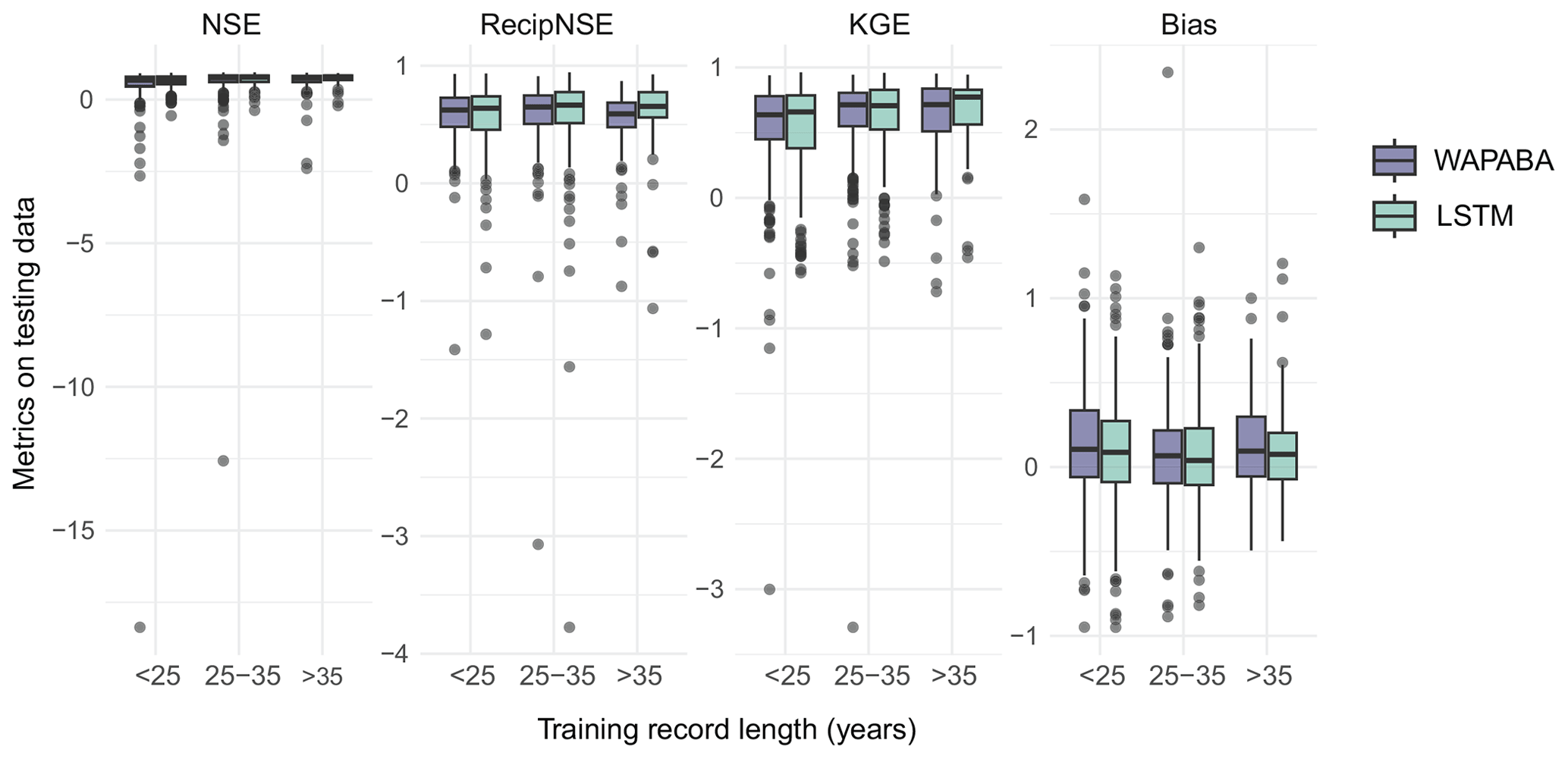
Figure A2 Effect of record length and training data size on prediction performance for each model type. A reproduction of Fig. 14 that includes outliers.

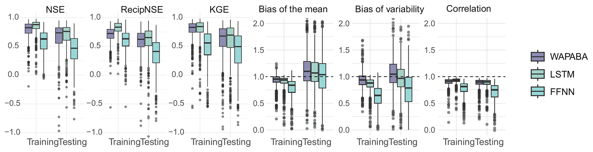
Figure A3 FFNN metrics compared with WAPABA and LSTM metrics, corresponding to Figs. 4 and 5.

Feed-forward neural network

To investigate the use of a very simple neural network, the FFNN was run for the 496 catchments. Input variables were the same as for the LSTM and WAPABA; however, 6 months of historical values were included with each training observation. A grid search on five random catchments was conducted to select learning rate and batch size. Out of a search space of $[\mathrm{8},\mathrm{16},\mathrm{32}]$ for batch size and $[\mathrm{0.1},\mathrm{0.01},\mathrm{0.001},\mathrm{0.0001}]$ for learning rate, a batch size of 16 and learning rate of 0.01 were chosen.

Figure A3 includes the FFNN model results in the comparison with LSTM and WAPABA results. The FFNN values are lower than WAPABA and LSTM indicating poorer runoff predictions over this set of catchments.