the Creative Commons Attribution 4.0 License.
the Creative Commons Attribution 4.0 License.
 | 20 Jan 2023
A snow and glacier hydrological model for large catchments – case study for the Naryn River, central Asia
Sarah Shannon
Anthony Payne
Jim Freer
Gemma Coxon
Martina Kauzlaric
David Kriegel
Stephan Harrison
In this paper we implement a degree day snowmelt and glacier melt model in the Dynamic fluxEs and ConnectIvity for Predictions of HydRology (DECIPHeR) model. The purpose is to develop a hydrological model that can be applied to large glaciated and snow-fed catchments yet is computationally efficient enough to include model uncertainty in streamflow predictions. The model is evaluated by simulating monthly discharge at six gauging stations in the Naryn River catchment (57 833 km2) in central Asia over the period 1951 to a variable end date between 1980 and 1995 depending on the availability of discharge observations. The spatial distribution of simulated snow cover is validated against MODIS weekly snow extent for the years 2001–2007. Discharge is calibrated by selecting parameter sets using Latin hypercube sampling and assessing the model performance using six evaluation metrics.
The model shows good performance in simulating monthly discharge for the calibration period (NSE is ) and validation period (), where the range of NSE values represents the 5th–95th percentile prediction limits across the gauging stations. The exception is the Uch-Kurgan station, which exhibits a reduction in model performance during the validation period attributed to commissioning of the Toktogul reservoir in 1975 which impacted the observations. The model reproduces the spatial extent in seasonal snow cover well when evaluated against MODIS snow extent; 86 % of the snow extent is captured (mean 2001–2007) for the median ensemble member of the best 0.5 % calibration simulations.
We establish the present-day contributions of glacier melt, snowmelt and rainfall to the total annual runoff and the timing of when these components dominate river flow. The model predicts well the observed increase in discharge during the spring (April–May) associated with the onset of snow melting and peak discharge during the summer (June, July and August) associated with glacier melting. Snow melting is the largest component of the annual runoff (89 %), followed by the rainfall (9 %) and the glacier melt component (2 %), where the values refer to the 50th percentile estimates at the catchment outlet gauging station Uch-Kurgan. In August, glacier melting can contribute up to 66 % of the total runoff at the highly glacierized Naryn headwater sub-catchment. The glaciated area predicted by the best 0.5 % calibration simulations overlaps the Landsat observations for the late 1990s and mid-2000s. Despite good predictions for discharge, the model produces a large range of estimates for the glaciated area (680–1196 km2) (5th–95th percentile limits) at the end of the simulation period. To constrain these estimates further, additional observations such as glacier mass balance, snow depth or snow extent should be used directly to constrain model simulations.
- Article
(14881 KB) - Full-text XML
-
Supplement
(21339 KB) - BibTeX
- EndNote


In High Mountain Asia, large populations rely on glacier and snow-fed river systems for their freshwater supply (Lutz et al., 2014; Armstrong et al., 2019). These “water towers”, which provide essential streamflow during the summer and a buffer against drought, are under threat as glaciers melt in response to warming temperatures (Kraaijenbrink et al., 2017; Immerzeel et al., 2013, 2010, 2020). The Aral Sea basin in central Asia has been identified as the region with the greatest human dependence on glacier meltwater (Kaser et al., 2010). Streamflow in the Syr Darya River, the second-largest river in central Asia, is supplied by snowmelt and glacier melt from the Tien Shan mountains during the spring and summer (Sorg et al., 2012). This water is crucial for hydro-production in upstream Kyrgyzstan and for irrigation downstream in the semi-arid lowlands of Kazakhstan and Uzbekistan.
Glaciers in the Tien Shan mountains have reduced in mass by approximately 27 % during the past 50 years (Pieczonka and Bolch, 2015). In the Naryn basin, the upstream tributary of the Syr Darya, satellite observations show a 23 % reduction in glacier area since the mid-1970s (Kriegel et al., 2013) and a similar reduction in the upper Naryn basin since the 1940s (Hagg et al., 2013). The shrinkage in glacier area has coincided with an increase in discharge in the upper reaches of the Syr Darya River caused by accelerated glacier melting (Zou et al., 2019). There has also been a shift in the precipitation regime, with more precipitation falling as rain and less falling as snow, leading to enhanced melting and less snow accumulation. Chen et al. (2016) showed that in the Tien Shan mountains the snowfall fraction decreased every decade, from 27 % in 1960–1969 to 25 % in 2005–2014.
As glaciers retreat, river runoff is expected to temporally increase, reaching a maximum known as “peak water”, after which flow is reduced as glaciers recede and disappear completely. There is a compelling need to predict the timing of “peak water” in order to understand when to implement adaption strategies in reduced river flow. Projections of future streamflow in the upper reaches of the Syr Darya River show a decrease during the summer and an increase in the spring as the hydrological regime shifts from one of glacier melting to seasonal snow melting (Radchenko et al., 2017). The reduction in summer streamflow will have direct impacts on water availability in the Ferghana Valley (Kyrgyzstan, Tajikistan) and further downstream in the Syr Darya River in Uzbekistan.
To estimate the timing of “peak water”, models which couple a representation of glacier processes to catchment hydrology are required. van Tiel et al. (2020) reviewed the many glacio-hydrological models in the literature and highlighted that one of the major challenges is uncertainty in the input data. Observations are generally sparse in mountainous regions. For example, meteorological stations are generally clustered at low altitudes, meaning that the derivation of the precipitation and temperature lapse rates can be very uncertain. Furthermore, observations of solid precipitation can be underestimated by 20 %–50 % due to windiness at high elevations (Rasmussen et al., 2012) which redistributes snow. The accuracy of streamflow predictions will also be affected by model structural uncertainty and uncertainty in model parameters that cannot be directly observed. Furthermore, the quality of discharge observations used to evaluate models is often difficult to determine. Incorporating uncertainty analysis into streamflow predictions means that the models we use need to be computationally efficient.
The treatment of snow and glacier melting in glacio-hydrological models can vary in complexity, from simple temperature index models (Neitsch et al., 2005; Zhang et al., 2013; Lindstrom et al., 1997), enhanced temperature index models (Ragettli and Pellicciotti, 2012; Mayr et al., 2013), to full energy balance models (Ren et al., 2018). A benefit of using a simple temperature index model is that only temperature is used to calculate melting, whilst energy balance models require observations of the radiation components, temperature, wind speed and humidity. This makes temperature index models a pragmatic choice for data-sparse regions, although it does mean that processes such as sublimation (important on glacier surfaces in areas of low humidity) might be overlooked. Furthermore, Magnusson et al. (2015) showed that for hydrological applications a temperature index model can predict daily snowpack mass and runoff as well as a more complex energy balance model.
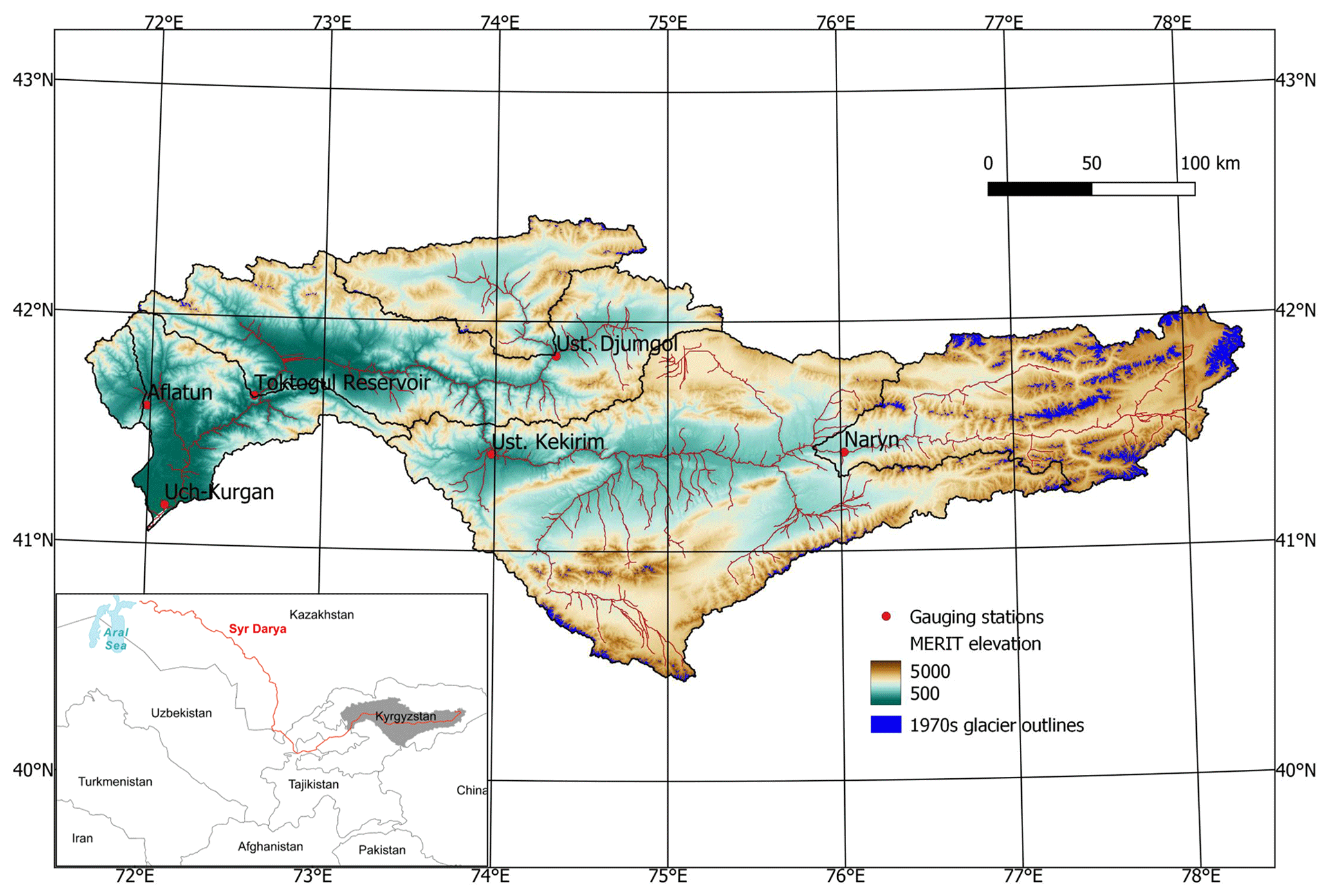
Figure 1The location of Naryn catchment and gauging stations. The MERIT DEM elevation and 1970s Landsat-derived glacier outlines used in this study are also displayed. The sub-catchment boundaries (black) and river path (red) calculated using DECIPHeR are shown. The Naryn River is a tributary of the Syr Darya River which flows across central Asia from the Tien Shan mountains to the remains of the Aral Sea (bottom left inset figure).
In this study, a degree day snowmelt and glacier melt scheme is incorporated into the Dynamic fluxEs and ConnectIvity for Predictions of HydRology (DECIPHeR) (Coxon et al., 2019) model. The aim is to develop a glacio-hydrological model that can be applied to very large glaciated catchments yet that still retains computational efficiency. This means that parametric uncertainty in streamflow predictions can be explored whilst retaining a high spatial resolution to allow orographic variability in the climate to be represented. Many glacio-hydrological models already exist in the literature (van Tiel et al., 2020; Horton et al., 2022); however, we integrate a snowmelt and glacier melt model into DECIPHeR for the following three reasons. Firstly, DECIPHeR uses hydrological response units (HRUs) to model water flow in hydrologically similar parts of the catchment and has a flexible model structure which allows the model to be run as a fully distributed (HRU for every single grid point), semi-distributed (multiple HRUs) or lumped model (1 HRU). Depending on user requirements and the corresponding degree of complexity, topographic, land use, geology, soil, anthropogenic and climate attributes as well as points of interest (any gauged or ungauged point on the river network) can be supplied to define the spatially connected topology and thus differences in model inputs, structure and parameterization (Coxon et al., 2019). Other HRU-based glacio-hydrological models exist, for instance, SWAT (Omani et al., 2017), PREVAH (Koboltschnig et al., 2008) and HBV (Finger et al., 2015), but they do not offer this level of flexibility within a single modelling framework. Secondly, DECIPHeR is computationally efficient, which makes it suitable for modelling very large catchments. Many of the glacio-hydrological models in the literature are distributed (grid point based), for example, TOPKAPI (Pellicciotti et al., 2012), DHSVM (Frans et al., 2018), VIC (Schaner et al., 2012) and GERM (Farinotti et al., 2012). The computational expense of modelling processes with adjacent grid points makes distributed models more suited to studying small catchments. Furthermore, computational efficiency makes it possible to quantify uncertainties and run large ensembles, which is important for understanding the uncertainties in future predictions. Thirdly, the DECIPHeR code is open source, which allows opportunities for further community development. In contrast, the glacier-enhanced version of SWAT (Omani et al., 2017; Luo et al., 2013b) is not open source.
The model performance is assessed by simulating discharge in the Naryn River catchment in central Asia for the period 1951–2007. Simulated snow cover is evaluated against MODIS remote sensing snow extent for the period 2001–2007. Simulated catchment-wide glaciated area is compared to glaciated areas derived from Landsat observations for time periods during the 1970s, 1990s and mid-2000s. This evaluation is used to establish the extent to which the model can reproduce past changes in river discharge, snow extent and catchment-wide glaciated area in order to have confidence in the model's predictive ability when applied to future scenarios. The model is used to quantify the present-day relative contributions of rain, snow and glacier melting to the total discharge and to determine the timing of when these components dominate river flow. Determining these baseline conditions for the present day is important because these will change in the future as the seasonal snowpack reduces and glaciers retreat. The paper is structured as follows. Sect. 2 gives an overview of the DECIPHeR model and describes the changes made to include the snow and glacier model. Section 3 describes the calibration and validation of discharge. Section 3.9 describes the validation of snow extent against MODIS observations. Section 4 describes the model limitations and proposes several avenues for further development.
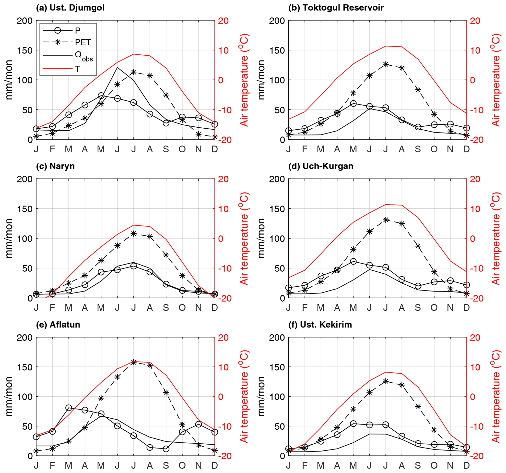
Figure 2Climatology of monthly mean temperature (T), potential evaporation (PET), precipitation (P) and observed discharge (Qobs) averaged for each sub-catchment for the calibration period 1951–1970. Temperature and PET are from the ERA5 and ERA5 back extension dataset, precipitation is from the APHRODITE dataset and observed discharge is from the Global Runoff Data Centre.
2.1 Study region
The Naryn River (Fig. 1) originates in the Tien Shan mountains in Kyrgyzstan and flows west through the Ferghana Valley into Uzbekistan, where it merges with the Kara Darya River to form the Syr Darya. The river is an important source of freshwater for agriculture downstream in the heavily irrigated Ferghana Valley (Radchenko et al., 2017). According to the Randolph Glacier Inventory Version 6 (RGI, 2017), there are currently 1784 glaciers in the catchment. Glaciers are found at elevations ranging between 2815 and 5125 m and are predominantly located in the east of the catchment and to a lesser extent in the north-west. Rock glaciers are also common above around 3000 m, especially downslope of contemporary glacier termini, and these represent considerable (if unquantified) ice and future water resources. The catchment has an area of 57 833 km2, of which 1060 km2 or 1.8 % is glaciated. The monthly temperature climatology (1951–1970) averaged over the catchment varies between −13 ∘C in January and +11 ∘C in August, and the majority of the annual precipitation falls in spring and early summer (April–July) (see Fig. 2d). There are six gauging stations with long-term monthly observations commencing in 1951 and terminating between 1980 and 1995 (see Sect. 3.1). Discharge at the six stations peaks in summer (June–August) due to glacier melting, with the exception of Aflatun, which is unglaciated and peaks sooner in spring (May) due to snow melting (Fig. 2).
For the purposes of this study, we assume that streamflow at the gauging stations has a natural signal. The exception is the Uch-Kurgan station, where streamflow after 1975 is impacted by the management of the Toktogul reservoir (Bernauer and Siegfried, 2012). A high-resolution irrigation map of the catchment derived from the normalized difference vegetation index (NDVI) (Meier et al., 2018) shows that the irrigated area is low (3 % area is irrigated), in contrast to the Ferghana Valley downstream (Fig. S1 in the Supplement). Irrigation is predominately clustered in the south-eastern part of the Naryn catchment.
2.2 DECIPHeR model
DECIPHeR is a flexible hydrological modelling framework (Coxon et al., 2019) which is based on the dynamic TOPMODEL (Beven and Freer, 2001; Metcalfe et al., 2015; Freer et al., 2004; Peters et al., 2003). The model can be spatially configured in any form, providing a distributed mosaic of interacting and spatially connected HRUs that allow different representations of water fluxes due to local conditions (i.e. geology, soils, slopes, vegetation) via different inputs (i.e. precipitation/evaporation), model structures and parameterizations. HRUs group together similar parts of the landscape to minimize run times of the model. This enables the user to run large ensembles of event data and climate simulations and provide probabilistic flow simulations essential for risk analysis. The user can use DECIPHeR to test different spatial configurations, from a fully gridded model to a lumped model set-up. Each HRU can be assigned its own processes and parameters, which allows for a more complex representation of spatially variable processes across the catchment. The capability to include spatially varying processes is particularly useful for modelling glaciers because the equations used to describe water storage and release from glaciated locations in the catchment will be different to unglaciated regions.
DECIPHeR simulates water storage, hydrologic partitioning and surface/subsurface flow for steeper shallow soils and/or groundwater-dominated watersheds. The model structure (as implemented in Coxon et al., 2019) consists of three stores defining the soil profile (root zone, unsaturated and saturated storage), which are implemented as lumped stores for each HRU. Moisture is added to the soil root zone by rainfall input and removed only by evapotranspiration. Any excess precipitation is added to the unsaturated zone, where it is either routed directly as overland flow or added to the saturated zone. Changes to storage deficits in the saturated zone are dependent on this recharge from the unsaturated zone, fluxes from upslope HRUs and downslope flow out of each HRU. Subsurface flows for each HRU are distributed according to a flux distribution matrix based on accumulated area and slope. Channel flow routing is modelled using a set of time delay histograms. For a more detailed discussion of the original DECIPHeR model structure, please see Coxon et al. (2019).
While DECIPHeR has been applied to catchments in the UK (Coxon et al., 2019; Lane et al., 2021), it has not been used for glacier or snow-fed rivers because cryospheric processes have not yet been included in the model. TOPMODEL, the forerunner of the dynamic TOPMODEL, did have a snowmelt scheme; however, seasonal variations in the degree day melt factor and snow sublimation were not included (Ambroise et al., 1996). DECIPHeR is implemented in two steps: (1) a digital terrain analysis (DTA) to set up and define the spatial complexity of the model domain and (2) ensemble simulation of that domain. The DTA is critical for defining the model complexity and landscape features that will separate HRUs, their equations, function types and parameterization. The DTA procedures also calculate the river network, routing path, catchment areas for each gauge and connectivity between the HRUs and HRUs to the stream network. More details on the DTA can be found in Coxon et al. (2019).
2.3 Modifications to the DECIPHeR model
The following sections describe the modifications made to the DECIPHeR model to include snow and glacier processes (for a full description of the hydrology included in DECIPHeR, see Coxon et al., 2019). We have altered the model to include a simple degree day snowmelt and glacier melt scheme. The degree day approach is a well-established method to calculate glacier and snow melting (Marzeion et al., 2020) and only requires air temperature as an input. The equations implemented in DECIPHeR for snowmelt and ice melt are similar to those in the SWAT model (Luo et al., 2013a). SWAT is one of the most widely used community hydrological models which have been applied to many snow-fed catchments (van Tiel et al., 2020). The evolutions of the snow and glacier depths are calculated every time step using the snow accumulation, melt and sublimation components. Temperature and precipitation are calculated at the HRU level by adjusting the gridded surface climate for elevation using a temperature lapse rate and a precipitation gradient. Glacier melt and snowmelt are added to the precipitation fields every time step and are then routed through the catchment. Figure 3 shows a conceptual diagram of the snow and glacier scheme added to the DECIPHeR model. All model parameters are sampled using Latin hypercube sampling.
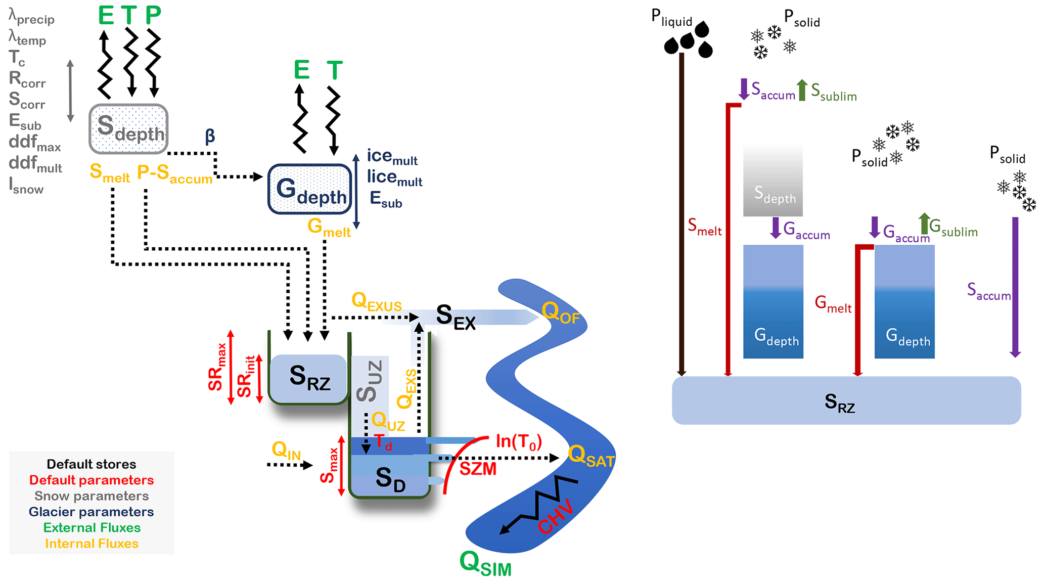
Figure 3Conceptual diagram of the model adapted from Coxon et al. (2019) to show snow and glacier stores and model parameters (left). Glacier ice is situated beneath the snowpack or can be exposed if no snowpack exits (right). The snowpack accumulates when precipitation falls in solid form. Liquid precipitation, snowmelt and glacier melt are transported to the root zone.
2.4 Modifications to the digital terrain analysis
The code is modified to read in two additional inputs: (1) air temperature, which is used for the degree day melting of ice and snow and to estimate the fraction of precipitation falling as rain or snow, and (2) the elevation of the forcing data which is used to apply a lapse rate correction to the surface temperature and precipitation fields. To reduce the number of HRUs, we do not classify glaciated regions as a function of accumulated area or slope, unlike in other parts of the catchment. HRUs located inside glaciers are only classified as a function of elevation, spatially varying climate and a unique ID that identifies the glacier. The spatial distribution of HRUs in the upper part of the catchment is shown in Fig. S2.
2.5 Modifications to the hydrological model
2.5.1 Snowpack model
The daily snowpack depth is calculated as
where Saccum, Smelt and Ssublim are the snow accumulation, melt and sublimation components at time step t and is the snow depth at the previous time step. The snowpack components are described below.
2.5.2 Snowpack melting
Melting is related to the snowpack temperature using a degree day factor for snow. The degree day factor accounts for a variety of different processes that control melting, such as the presence of debris cover or the darkening of snow through the snow aging process. The potential snowmelt Smelt (m w.e. d−1) is
where Tsnow is the snowpack temperature (∘C), ddfsnow is the degree day factor for snow melting (m w.e. ∘C−1 d−1) and Tmelt is the melt temperature. To reduce the number of parameters required to calibrate the model, we assume that Tmelt=0 ∘C. A criterion is enforced such that the melting depth cannot exceed the depth of snow that exists.
A seasonally varying degree day factor is calculated which has a maximum snowmelt on 21 June (ddfmax) and a minimum snowmelt on 21 December (ddfmin). The reason to use a seasonally varying degree day factor rather than a constant one is because the degree day factor is a simplification of processes that can be more correctly described by the energy balance, i.e. inward and outward longwave and shortwave radiation, albedo, and latent and sensible heat, which vary throughout the year and are not solely a function of temperature. The degree day factor is represented as a sinusoidal curve,
where j is the day of the year.
The ddfmin is calculated by multiplying the maximum value by a scale factor ddfmult.
The scale factor can vary between 0 and 1 and ensures melt rates are lower in the winter than in the summer.
The temperature of the snowpack Tsnow is calculated from the air temperature using a lag factor lsnow. The lag factor can vary from 0 to 1, where a value of 1 sets the snowpack temperature equal to the air temperature. A value less than 1 sets the snowpack temperature lower than the air temperature. Using a temperature lag factor is a simple way of approximating the snowpack temperature without doing more complex heat transfer modelling of the temperature flux from the air into the snowpack. The lag factor accounts for affects of snow depth and density on the snowpack temperature.
where is the snowpack temperature at the previous time step.
The daily HRU temperature Thru (∘C) is calculated by adjusting the forcing temperature T0 (∘C) using a lapse rate λtemp (∘C m−1).
where Ehru is the elevation of the HRU (m) derived from a digital elevation model (DEM) and Eclimate is the elevation of the forcing data (m). Calculating temperature at the HRU level allows us to downscale the gridded climate data, allowing for high-resolution spatial variability in temperature as a function of elevation.
2.5.3 Snowpack accumulation
Snow accumulates in the snowpack when precipitation falls in the form of snow.
where Saccum is the snow accumulation (m w.e. d−1), Psolid is the solid precipitation falling on the HRU (m w.e. d−1) and Tc is the threshold temperature for the conversion of rain to snow (∘C).
A spatially uniform rainfall and snowfall correction factor is applied to the precipitation based on the equations used in the HBV-ETH model (Mayr et al., 2013). The correction is applied because gridded datasets often underestimate precipitation in mountainous regions due to the lack of meteorological stations at high elevations and the fact that observations of solid precipitation are susceptible to undercatch due to windy conditions (Rasmussen et al., 2012). Wortmann et al. (2019) demonstrated using the Soil and Water Integrated Model–Glacier Dynamics (SWIM-G) model that the APHRODITE precipitation (used in this study) needed to be increased by a factor of 1.5–4.3 to maintain observed glacier area and mass balances. Solid and liquid precipitation are scaled separately:
where Ps and Pl is the scaled solid and liquid precipitation (m d−1), P0 is the forcing precipitation (m d−1), Sc and Rc are dimensionless snowfall and rainfall correction factors. Solid and liquid precipitation are lapse rate corrected for elevation using a linear precipitation gradient. The solid precipitation Psolid falling on the HRU (m d−1) is
where λprecip is the precipitation lapse rate (% m−1). The liquid precipitation falling on the HRU Pliquid (m d−1)
Rain falling on a snow- or ice-covered HRU is passed to the root zone.
2.5.4 Snowpack sublimation
The quantity of snow sublimated is calculated using the potential evapotranspiration which is provided as an input forcing dataset. The parameter Esub is used to reduce the potential evapotranspiration over snow surfaces. Sublimation is then set equal to the reduced PET, and no PEThru is passed to the root zone.
Ssublim is the snow sublimation (m w.e. d−1), PEThru is the forcing data potential evapotranspiration (m d−1) and Esub is a parameter to be calibrated that reduces the evapotranspiration over snow-covered HRUs. Using PET to approximate snow sublimation has also been implemented in the SWAT model (Fontaine et al., 2002).
2.5.5 Glacier model
The daily glacier depth is
where Gaccum, Gmelt, and Gsublim are the glacier accumulation, melt and sublimation components at time step t and is the glacier depth at the previous time step.
2.5.6 Glacier melting
When the snowpack has melted and the glacier ice is exposed, melting can occur. The amount of glacier ice melted Gmelt (m w.e. d−1) is
where ddfice is the degree day factor for ice melting (m w.e. ∘C−1 d−1), Tglacier is the temperature of the glacier ice (∘C), Tmelt is the melt temperature which is set to 0 ∘C.
The degree day factor for ice is calculated from the degree day factor for snow by multiplying by a scaling parameter icemult. The scaling parameter increases the degree day factor for ice relative to snow. Ice generally melts more per degree day than snow because it has a lower albedo.
Glacier temperature is related to the air temperature using a lag factor
where Tglacier is the glacier temperature (∘C), T0 is the glacier temperature at the previous time step (∘C), Thru is the lapse-rate-corrected temperature of the HRU (∘C), lglacier is the dimensionless lag factor for ice. The lag factor for glacier ice is found by multiplying the lag factor for snow by a scale factor . This reduces the temperature lag factor for ice relative to snow, because ice responds more slowly to the air temperature than snow.
2.5.7 Glacier accumulation
Glacier accumulation is calculated by transforming a fraction of the snowpack into glacier ice. This is a simple way of converting snow into ice without including more complex processes such as the densification and compaction of snow grains under the force of gravity. Glacier accumulation is
where (β) is the basal turnover coefficient (d−1). This represents the fraction of snow that is removed from the snowpack and converted into ice every time step. The minimum parameter range for β is 1 year ( d−1), which means that it takes 1 year for all of the snowpack to be converted into ice. The upper bound is 100 years ( d−1). The upper range is based on observations of the age of ice at the firn–ice transition depth for different glaciers (Paterson, 1994).
2.5.8 Glacier sublimation
Sublimation occurs when the snowpack has disappeared and the glacier ice is exposed. We assume that the reduction in PET over snow and ice surfaces is the same.
where Esub is used to reduce the potential evapotranspiration over ice and snow HRUs. Sublimation is set to the reduced potential evapotranspiration value.
2.5.9 Snowmelt and glacier melt contributions to streamflow
Water from snow and glacier melting is added to the precipitation field and routed through the model to simulate river discharge.
where Ptotal is the total water input to the catchment, Pliquid is the liquid precipitation on the HRU, Smelt is the snowmelt contribution and Gmelt, each with units (m w.e. d−1). See Table 3 for a list of the model parameters that are calibrated.
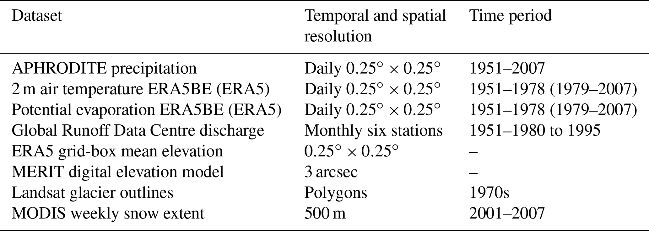
3.1 Input data for DECIPHeR
DECIPHeR requires a digital elevation model and information on the locations of gauging stations. Catchment elevation data are provided by the Multi-Error-Removed Improved-Terrain (MERIT) digital elevation model (Yamazaki et al., 2017). The DEM has a spatial resolution of 3 arcsec (∼90 m at the Equator) and is pre-processed to remove any sinks or flat areas. Therefore we assume that all of the catchment area flows to the gauging outlets.
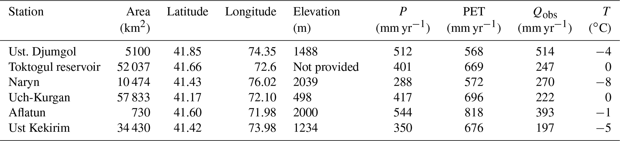
The location of the gauging stations and monthly discharge observations come from the Global Runoff Data Centre (GRDC). There are six gauging stations located the Naryn River catchment: Djumgol, Kekirim, Naryn, Toktogul reservoir, Aflatun, and Uch-Kurgan (Table 2). The Toktogul reservoir gauging station is located immediately upstream of the reservoir dam and so is not affected by water abstraction. Discharge at the Uch-Kurgan station after 1975 is impacted by the reservoir management. Table 1 contains a list of the input and evaluation datasets used in this study.
Table 2The location, catchment area and elevation of the gauging stations from the Global Runoff Data Centre. Also listed are the annual mean climatologies (1951–1970) for APHRODITE precipitation (P), ERA5 potential evapotranspiration (PET), ERA5 air temperature (T) and observed discharge (Qobs).
3.2 Glacier area and thickness
Glacier outlines are used in the model to identify glaciated/non-glaciated HRUs and initial glacier thicknesses for each HRU. These are calculated using glacier outlines derived from Landsat Multispectral Scanner imagery for the 1970s (Kriegel et al., 2013). According to the Landsat data, 1472 glaciers existed in the catchment during the 1970s. Determining glacier thicknesses at the start of the simulation is problematic due to the lack of long-term observations. Therefore, we infer glacier thickness using the Glacier bed Topography (GlabTop2) method (Frey et al., 2014), where the glacier outlines from the 1970s and the MERIT DEM are used as input. Freely available python code to implement the GlabTop2 method was obtained from https://pypi.org/project/GlabTop2-py (last access: 17 December 2020). Glacier thicknesses are converted to units of m w.e. using an ice density of 917 kg m−3.
GlabTop2 is a useful technique to infer glacier thicknesses in the absence of observations; however, the method has some limitations that should be acknowledged. Firstly, the method uses a simple parameterization for the basal shear stress based on the elevation difference within a glacier. This can introduce a source of uncertainty into the initial ice thicknesses. Secondly, the method can produce very high ice thicknesses for locations with low slopes. Low slopes can appear in the MERIT DEM if a glacier has retreated and a glacier lake is formed or an existing lake expands. Two glaciers in the upper part of the catchment have very low slopes (flat) at the terminus and large ice thicknesses. The larger of these is Petrov Glacier which drains into the Petrov glacial lake. Observations show that Petrov Glacier has experienced accelerated retreat since the 1970s (Engel et al., 2012), and the lake area has more than doubled since 1980 (Janský et al., 2010). To correct for this, we take the mean thickness of a 5×5 pixel buffer upstream of the terminus for each of the two glaciers and replace the large thickness values with the fill value. Ice thicknesses before and after the fill values have been applied can be seen in the Supplement (Figs. S3 and S4, respectively). A third limitation is that the thickness estimate uses 1970s outlines, but our model simulations commence in 1951. In situ mass balance observations show that glaciers in the Tien Shan were in a quasi-stable state between the 1950s and the 1970s but experienced accelerated mass loss in the years that followed (Barandun et al., 2020; Liu and Liu, 2016). The glaciers in the aforementioned studies were located outside of the Naryn catchment; however, we assume that the mass balance trends are representative of our study region.
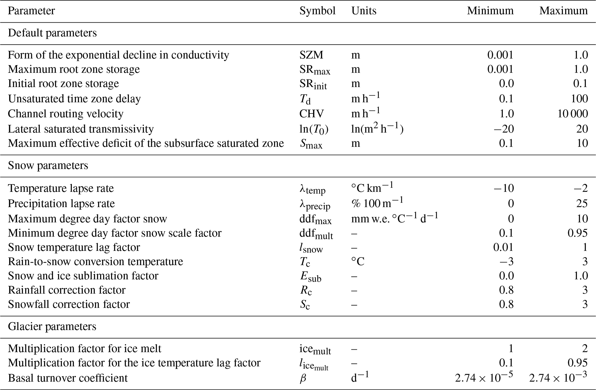
Table 3List of parameters and ranges. Default parameters are described in detail in Coxon et al. (2019). The glacier and snow parameters have been added to the model for this study.
3.3 Input climate
Daily precipitation data are provided by the Asian Precipitation Highly-Resolved Observational Data Integration Towards Evaluation of Water Resources (APHRODITE) Russia and Monsoon Asia V1101 daily precipitation (Yatagai et al., 2012). These data have been shown to outperform other gridded precipitation datasets for hydrological modelling applications in central Asia (Malsy et al., 2015). The APHRODITE data are constructed from a network of rain gauges across Asia which are interpolated onto a 0.25∘ grid. Daily air temperature, potential evaporation and elevation of the climate data come from the ERA5 back extension (ERA5 BE) 1950–1978 and ERA5 1979–2007 (Copernicus, 2017). These data have a spatial resolution of .
3.4 Calculation of hydrological response units
HRUs are calculated by categorizing the catchment according to the following.
-
81 elevation ranges consisting of 0–2000 m in increments of 100 and 2000–5200 m in increments of 50 m. These elevation bands are selected to downscale the temperature and precipitation which is used for snow and glacier model. The finer 50 m bands are used between elevations 2000 and 5200 m because glaciers are located within these elevation ranges in the catchment.
-
Dividing the non-glacierized parts of the catchment into three equally sized surface slope and accumulated area fractions. This results in HRUs that cascade down to the valley bottom.
-
Spatially varying precipitation, temperature and potential evapotranspiration. This provides the model with a regionally varying climate forcing.
-
Glacier mask which is used to determine if a HRU is initially glacierized or non-glacierized.
This categorization results in the following variable spatial resolution characteristics: a mean area of 0.94 km2, median 0.27 km2, minimum 0.0055 km2 and maximum 259.93 km2 per HRU. (See Fig. S5 for a histogram of the areal distribution of the HRUs.) The total number of HRUs in the catchment is 61 481.
3.5 Initialization and spin-up
The initial snowpack depth is set to 0 m w.e., and its temperature is set to 0 ∘C. The initial glacier temperature is set to −5 ∘C. The calculation of the initial glacier thicknesses using the GlabTop2 method is described in Sect. 3.2. The model is spun up by repeating the first simulation year 1951 for 10 years. The spin-up time period is found by performing an idealized experiment in which precipitation forcing is kept constant through time and the temperature forcing is set to less than 0 ∘C to ensure there is no snow or ice melting. Under these conditions, the discharge reaches an equilibrium in approximately 10 years.
3.6 Calibration and validation of discharge
The model is calibrated for the period 1951–1970 to determine behavioural parameter sets, and then these are validated for the period 1971 to a variable end date between 1980 and 1995 depending on the availability of discharge observations at each gauging station. The calibration period is prior to the commissioning of the Toktogul reservoir in 1976 which affected the discharge at Uch-Kurgan. The model is run on a daily time step and monthly simulated discharge is calculated from daily values. Twelve additional parameters are added to DECIPHeR for the snow and glacier scheme. The parameters and their minimum and maximum sampling ranges are listed in Table 3. In total, 150 100 simulations using parameter combinations selected using Latin hypercube sampling are run (McKay et al., 1979). This form of stratified sampling is a more efficient and structured approach to generating a “near-random” sample for large multi-dimensional problems such as this. Model performance is assessed using the six evaluation metrics described in Sect. 3.7 below. The best 0.5 % performing simulations (see the section below for the methods) in the calibration period are used in the validation.
3.7 Generalized likelihood uncertainty estimation (GLUE)
GLUE is a technique used to identify parameter sets which provide a good representation of the system (Beven and Binley, 1992; Freer et al., 1996; Beven, 2006). The approach assumes that there is no single optimum parameter that can be considered correct, but instead there is a set of “behavioural models” that describe the system equally well. In this study, we want to select models that perform well in simulating seasonal changes in discharge. The onset of snow melting affects the discharge during the spring, whereas peak discharge during the summer is affected by glacier melting. It is equally important to ensure that the model performs well during the autumn and winter. Station observations show that the warming in the Naryn basin over the period 1960–2007 occurred primarily during autumn and winter (Kriegel et al., 2013). Warming winter temperatures cause a reduction in snowpack accumulation when more precipitation falls in the form of rain rather than snow. This has an impact on the autumn and winter hydrograph. Therefore we use the following metrics to assess the model performance.
The Nash–Sutcliffe efficiency (NSE) is used to evaluate high flows and the timing of peak discharge, particularly from glacier melting during the summer. NSE values range between −∞ and 1 where NSE=1 is the optimal value.
and is observed and simulated monthly discharge, is the mean observed monthly discharge and n is the number of observations.
The bias in runoff ratio PBIAS is a measures of the tendency of the simulated data to be larger or smaller than the observations (Yilmaz et al., 2008). A negative PBIAS indicates the model underestimates the discharge and a positive bias indicates the model overestimates the discharge. PBIAS close to zero indicates better model performance.
The ratio of the root mean square error to the standard deviation of the observations (RSR) (Moriasi et al., 2007) is used to evaluate the model performance for the four seasons, and therefore this provides four separate evaluation metrics (bringing the total to six).
where i is discharge for the months of spring (March, April, May), summer (June, July, August), autumn (September, October, November) and winter (December, January, February). is the mean of the observed discharge. Better parameter sets have lower values of RSR. The units of RSR are dimensionless which makes it useful for comparing the model performance between the sub-catchments and with other studies.
In this study two different calibration techniques are tested.
-
ISC: individual-site calibration to find parameter sets best suited to individual sub-catchments. This approach parameterizes areas upstream of a gauge in a lumped way. This is different to the step-wise approach where each upstream to downstream catchment is calibrated sequentially, resulting in spatial differences between upstream–downstream parameters. Nonetheless, the ISC method allows us to identify the spatial variability in parameters across the catchment.
-
MSC: multi-site calibration to find global parameters sets suited to the entire catchment.
The purpose of using two approaches is to investigate whether there are parts of the catchment that behave differently to the entire catchment. The results of ISC are included in the main body of the paper and the results of MSC are detailed in the Supplement.
Model performance is assessed by calculating conditional probabilities from the six metrics described above. The final conditional probability values are combined with an equal weighting to give overall model performance, where higher conditional probability values (after all the normalization steps) indicate better model performance. Prior to calculating the conditional probability values, NSE values less than zero are set to zero. By doing so, we reject these simulations because they will have a zero conditional probability. The NSE is adjusted such that
This ensures that NSE values closer to zero represent good model performance and values closer to 1 represents poorer model performance. The absolute value of PBIAS is also calculated |PBIAS|. No prior adjustments are required for RSRseason because values close to zero are already considered good.
The metrics NSErev, |PBIAS| and RSRseason are normalized so that values vary from 0 (good performance) to 1 (poor performance). This is to account for the difference in units between the metrics and the fact that the upper bounds values for the metrics are different. PBIAS has units of percent and RSRseason and NSErev have dimensionless units. The upper bound value for NSErev and RSRseason is 1, whilst PBIAS can have an upper bound value exceeding 1. The above metrics are then normalized so that they are all on a scale of 0 to 1:
where is the metric m at catchment c for simulation i and I=(1, 2, …, n) are the vector of simulations from 1 to the number of simulations n. and are the maximum and minimum values of the metrics across all simulations for each catchment.
Once normalized, the values for each simulation, for each metric, and for each catchment are then calculated as
so that a higher value (between 0 and 1) reflects a better simulation for that metric. Finally the conditional probability values are then calculated so that for each metric and for each catchment all the simulations sum to 1.
where n is the number of simulations. For the ISC method, a combined conditional probability measure is calculated for each sub-catchment (Θc,i) by multiplying the conditional probability measures derived from the six metrics. We assume the metrics contribute equally to the overall model performance.
For the MSC method, catchment-wide conditional probability measures are calculated by multiplying Θc,i for each sub-catchment. We assume that the sub-catchments contribute equally to model performance.
Simulations are ranked in order of descending conditional probability measure, where maximum values indicate good model performance. The best performing 0.5 % calibration simulations (n=751) are extracted and used to validate the discharge and spatial snow extent.
3.7.1 Individual site calibration and validation
Figures 4 and 5 show the simulated and observed discharge for the calibration and validation periods using the best 0.5 % simulations. The ranges of values for the performance metrics are listed in Table 4. For the calibration period the model is able to capture the seasonal peaks in discharge well, with NSE values for the 5th–95th prediction limits and PBIAS values lower than 11.36 % at all the gauging stations. RSR values can be considered “satisfactory” (RSR<0.7) during the winter, spring and autumn; however, some RSR values exceed 0.7 in the summer (June, July, August) indicating poorer model performance when glacier melting is active.
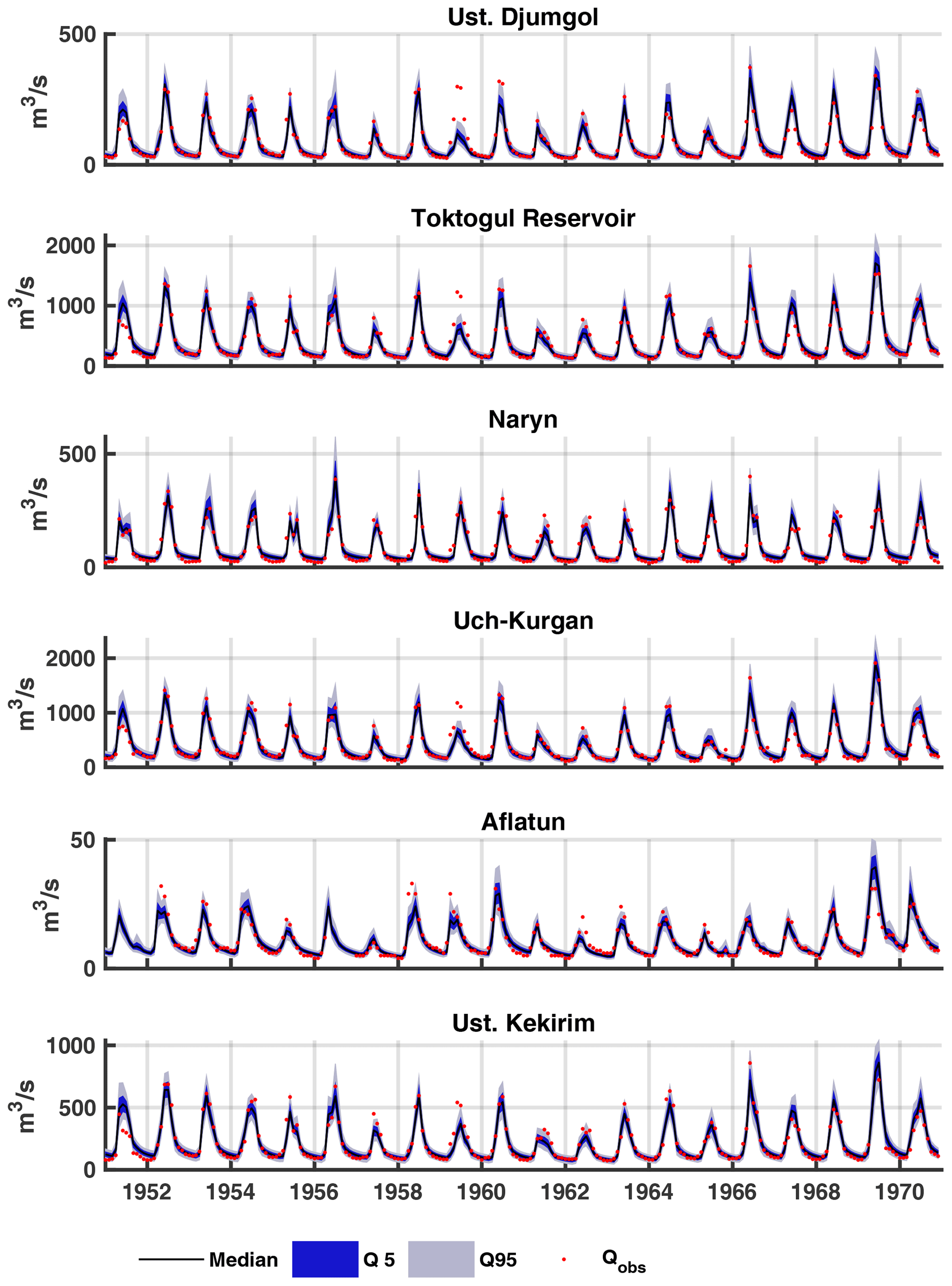
Figure 4Observed and simulated discharge for the calibration period when parameters are selected for individual sub-catchments (MSC method). The shaded envelopes show the 5th–95th percentile ranges and the black line shows the 50th percentile of the best 0.5 % simulations.
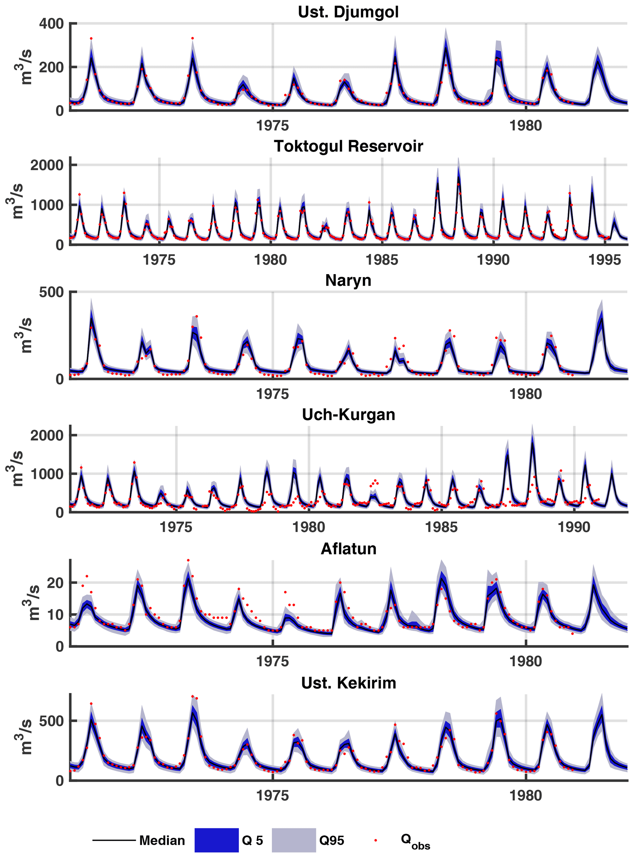
Figure 5Observed and simulated discharge for the validation period when parameters are selected for individual sub-catchments (MSC method). The shaded envelopes show the 5th–95th percentile ranges and the black line shows the 50th percentile of the best 0.5 % simulations.
Table 4Calibration and validation performance metrics for the best 0.5 % of the ensemble (751 simulations) when parameters are selected for individual sub-catchments. The table lists the metrics for the best simulation and the 5th, 50th and 95th percentile limits.

For the validation period the model also performs well NSE values for the 5th–95th prediction limits, with the notable exception of the Uch-Kurgan station where discharge is overestimated by up to 32 %. The discrepancy is most noticeable during the summers of 1987 and 1988. The model simulates the observed peak discharge during these years well at the Toktogul reservoir gauging station, which is located upstream of the reservoir; however, downstream of the reservoir at Uch-Kurgan, discharge is overestimated. Observations from the Central Asian Waterinfo Database shows that the reservoir inflow was very high during these 2 years, which coincided with a sharp increase in the reservoir volume by 7253 million m3 from August 1987 to August 1988 (Fig. S6). Initial and calibrated parameter ranges for each sub-catchment for the best 0.5 % of ensemble are listed in Table S3.
3.7.2 Multi-site calibration and validation
Simulated discharge for the calibration and validation periods is shown in Figs. S7 and S8, and performance metrics are listed in Table S1 in the Supplement. There is a degradation in model performance when the MSC method is used to calibrate the model (see Table S1). The reduction in model performance is most noticeable for the Naryn sub-catchment, where the best NSE is 0.91 for the ISC method and 0.59 for the MSC method. Furthermore, the summer peaks in discharge at the Naryn sub-catchment are underpredicted when using the MSC method to select global parameters (Fig. S8). This suggests that the global catchment parameters are not well suited to the Naryn sub-catchment. Dotty plots showing the conditional probability values for the model parameters are shown in Fig. S9 (MSC method) and Figs. S10–S15 (ISC method). The top 10 best simulations are shown in red triangles.
Simulations that perform well in the sub-catchments (Figs. S10–S15) favour higher values for the precipitation lapse rates, in contrast to the global catchment parameters which range from 1 % 100 m−1 to 10 % 100 m−1 (Fig. S9). This is visible in Table S2 which summarizes the range of precipitation lapse rates for the 10 best-performing simulations for each sub-catchment. The upper values for the precipitation lapse varies between 16 % 100 m−1 and 24 % 100 m−1 depending on the sub-catchment, which is higher than the global catchment upper bound of 10 % 100 m−1. Simulations also perform better in the sub-catchments when higher values for the sublimation factor Esub are used, in contrast to the global values (0.005–0.2). The 10 best Esub parameter ranges are also listed in Table S2. The upper bound values for Esub vary between 0.6 and 1.0, depending on the sub-catchment, which is higher than 0.2 predicted by the global catchment values. Esub controls the reduction in PET over snow and ice surfaces. This indicates that discharge in the Naryn is predicted better when PET is reduced. The PET has not been adjusted for elevation, unlike the air temperature and precipitation. The ERA5 PET has a 0.25∘ spatial resolution, which is much larger than the HRU areas. In mountainous regions PET should decrease with height as a consequence of decreasing temperatures (Lambert and Chitrakar, 1989).
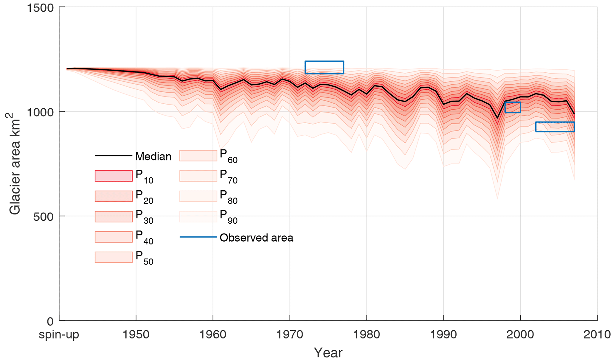
Figure 6Simulated (top 0.5 %, n=751) catchment-wide glaciated area using parameters for the Ust. Kurgan station which is located at the outlet of the catchment. The Landsat-observed glaciated area (Kriegel et al., 2013) is shown in blue boxes, where the error on the time axis relates to the years when satellite imagery was used to calculate area. The Landsat-glaciated area uses satellite imagery from the 1970s (1972–1977), late 1990s (1998–2000) and mid-2000s (2002–2007). A simulated threshold glacier depth of 1 mm is used to identify the presence of glacier ice. The figure shows the spread of the glaciated areas predicted by the model, but the simulations are not sorted by conditional probability values.
We used wide parameter ranges to calibrate the model because this is the first time applying DECIPHeR in a mountainous region, with snowmelt and glacier melt processes included. The dotty plots (see Fig. S9) show that the sampled parameter ranges could be further reduced for two of the parameters; the lateral saturated transmissivity (ln (T0)) and the rainfall correction factor (Rc). The ln (T0) calibration range is −20 to 20 ln(m2 h−1); however, the best simulations have values that are predominately clustered around −7 and 0. Rc is calibrated between 0.8 and 3, but the best simulations have values of less than 2. To explore whether any of the parameters are correlated, a plot of the coefficient of determination (r2) for parameter pairs is shown in Fig. S16 for the best 0.5 % calibration experiments. The strongest correlation is found between the precipitation lapse rate and the snowfall correction factor (r2=0.46), which both control the quantity of snow accumulation. The correlation indicates that good simulations can be produced with higher values of snowfall correction factor combined with lower precipitation lapse rates or vice versa.
3.8 Validation of the glaciated area against Landsat observations
The simulated catchment-wide glaciated area is compared to the Landsat-derived glaciated area (Kriegel et al., 2013) for the best 0.5 % calibration simulations. The Landsat glaciated area is available for three time periods: the 1970s (1972–1977), which were used to calculate initial glacier thicknesses using GlabTop2, the late 1990s (1998–2000) and the mid-2000s (2002–2007). The observations have an uncertainty bound associated with the delineation process which was calculated by placing a buffer of approximately 1 pixel wide (for example, 79 m for observations in the 1970s) around the glacier polygons. The uncertainty is the difference between the glaciated area and the area extended by the buffer. Figure 6 shows the simulated glaciated area for the top 0.5 % simulations in the calibration overlaid with the Landsat observations. The simulated glaciated area overlaps the Landsat observations in the late 1990s and mid-2000s. The model produces a large range of estimates for the glaciated area (680–1196 km2) (5th–95th percentile limits) at the end of the simulation period. This range is larger than the observed uncertainty range of 903–948 km2. The uncertainty range in the model is 516 km2 (in 2007), which is more than 10 times greater than the uncertainty in the observed glaciated area (46 km2).
Figure 7 shows the initial glacier thickness and the mean annual thickness at the end of the simulation period in 2007 for a region in the upper part of the catchment. A thinning of the glaciers and retreat of the terminus from the initial glacier outlines in 1970 is evident. The plots show the median ensemble member of the best 0.5 % calibration simulations.
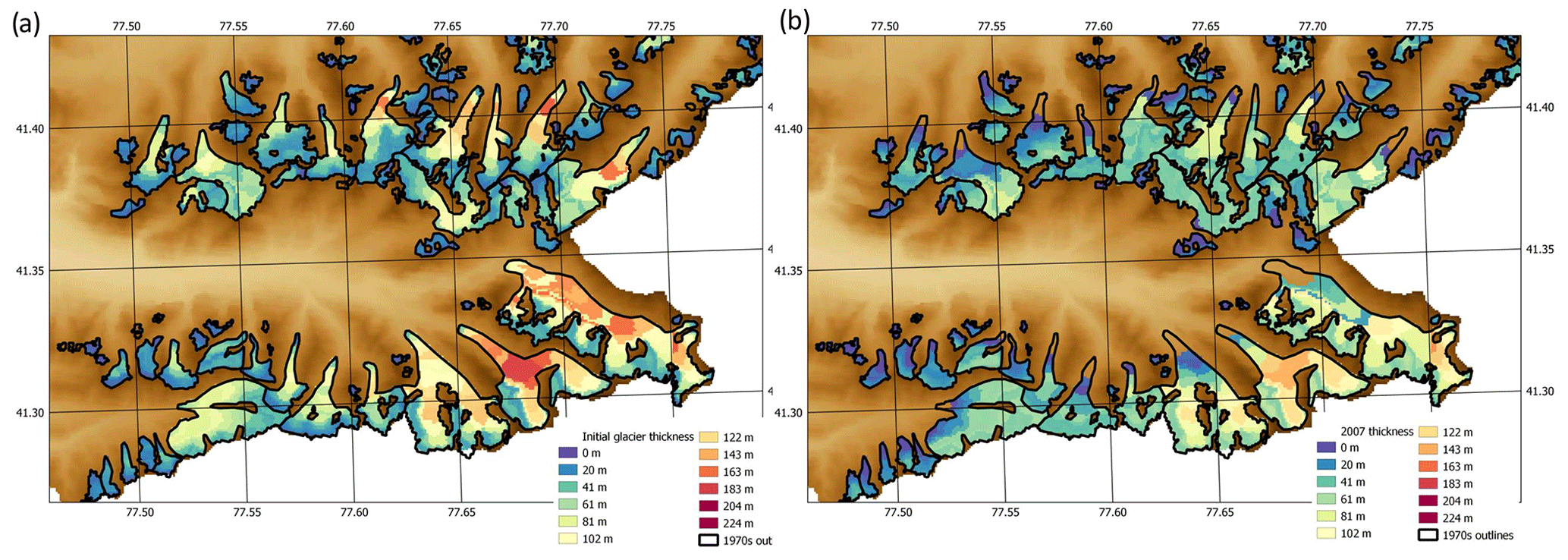
Figure 7Panel (a) shows initial glacier thicknesses on HRUs calculated using GlabTop2 in the upper part of the Naryn catchment. 1970s glacier outlines are shown in black. Panel (b) shows the annual mean thickness for the year 2007 for the median ensemble member in the top 0.5 % calibration simulations.
3.9 Validation of modelled snow extent against MODIS observations
We evaluate the simulated spatial distribution of snow extent against MODIS 500 m resolution 8 d snow cover extent MOD10A2 version 6 (Hall and Riggs, 2016) for the period 2001–2007. Snow extent is an internal hydrological variable that was not used in the calibration and is complementary to the discharge time series, which is spatially integrated. MODIS snow extent does not contain information on the snow water equivalent; however, it is spatially distributed, which makes it particularly useful for the evaluation of distributed models (Duethmann et al., 2014; Finger et al., 2011).
Daily simulated snow depth for each HRU is output for three simulations from the best 0.5 % calibration simulations: 50th (median), 5th and 95th ensemble members. It was not feasible to output daily HRU snow depth for all 751 simulations due to the size of the data. Snow depth is converted from metres of water equivalent to metres using a density of 300 kg m−3, which is the mean density of settled snow. A spatial map of snow depth is generated by converting the snow depths on HRUs to a spatial grid using a map of HRU locations which was generated by the digital terrain analysis.
The MODIS sensor detects snow in a pixel if there is any snow present within an 8 d period. To compare this to the model output, we assume snow is present in the model if the snow depth exceeds 1 cm on any day within the 8 d MODIS observational period. This threshold is used because MODIS can begin to detect snow with an accuracy 40 % (Pu et al., 2007) at this depth. Modelled snow extent is interpolated onto a 500 m grid for direct comparison with the MODIS data. Pixels where the MODIS data detect cloud cover are excluded from the analysis. Seasonal MODIS and simulated snow extent is calculated from the weekly data by selecting all the weeks that occur during a season and finding the most frequent state (i.e. snow or no-snow) for each pixel.
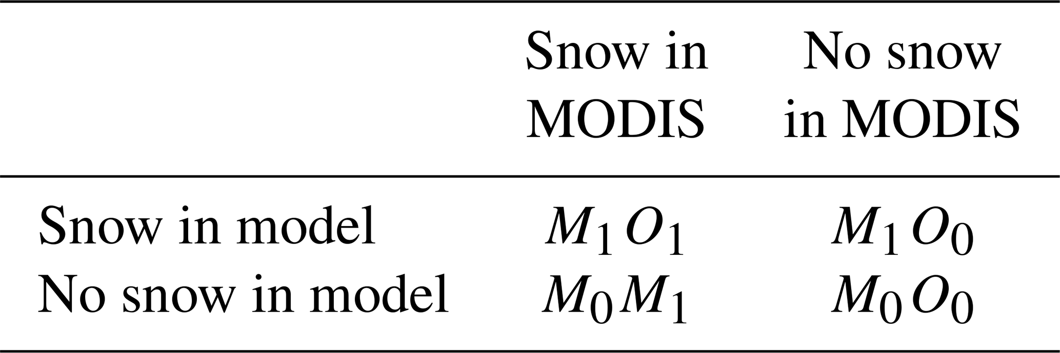
For each season, a binary classification scheme is used to enable a comparison between the MODIS and modelled seasonal snow extent. The classification scheme has been used in flood hazard modelling to validate simulated and observed flood hazard area maps (Wing et al., 2017). Four metrics of fit are used, which categorize the relative number of pixels which conform to one of the states in the contingency table (Table 5).
Table 5Table of possible pixel states in a binary classification scheme for the validation of seasonal MODIS (O) and modelled (M) snow extent.
The first is the hit rate (H), which is the proportion of snow pixels in the MODIS data that were reproduced by the model.
H can range from 0 (none of the snow pixels in the MODIS data are snow pixels in the model data) to 1 (all of the snow pixels in the MODIS data are snow pixels in the model data).
The second metric is false alarm ratio (F), which indicates the proportion of snow pixels in the modelled that are not snow in the MODIS data.
F can have values ranging from 0 (no false alarms) to 1 (all false alarms). F evaluates the tendency of the model to overpredict the snow extent.

Figure 8Spatial distribution of the hits, misses and false alarms between the simulated snow extent (median 50th percentile simulation) and MODIS snow extent for the year 2002. Hits, misses and false alarms are defined in Table 5.
The third is the critical success index (C), which evaluates both overprediction and underprediction in the model and can range from 0 (no match between modelled and MODIS data) to 1 (perfect match between modelled and MODIS data).
The fourth is the error bias (E) which evaluates the tendency of the model to underpredict or overpredict snow extent.
E=1 indicates no bias, indicates a tendency toward underprediction, and indicates a tendency toward overprediction.
The spatial distribution of the hit rates, misses and false alarms are shown in Fig. 8 for the median (50th percentile simulation) of the best 0.5 % calibration runs. (See Figs. S17 and S18 for the 5th and 95th percentile limit simulations.) Seasonal hit rates, misses and false alarms averaged over the years of MODIS observations 2001–2007 are summarized in Table 6. Seasonal snow extent is predicted reasonably well with mean hit rates exceeding 0.86 (median ensemble member). The model captures the complete snow cover observed in winter and the snow that persists at high elevations in the upper part of the catchment in the summer. Most noticeable is the poorer model performance in autumn, where there is a large positive bias (33.53 % median ensemble member) and a high number of false alarms (0.42 median ensemble member). This indicates that the model is overpredicting the snow extent in autumn. The best 0.5 % calibration simulations produce good estimates for discharge but at the same time predict a range of snow extent values. This can be seen in the fraction of the catchment covered in snow (Fig. 9) where NSE values range from 0.78 to 0.89 (95th–5th percentile limits simulations), with most of the model uncertainty occurring in the winter.
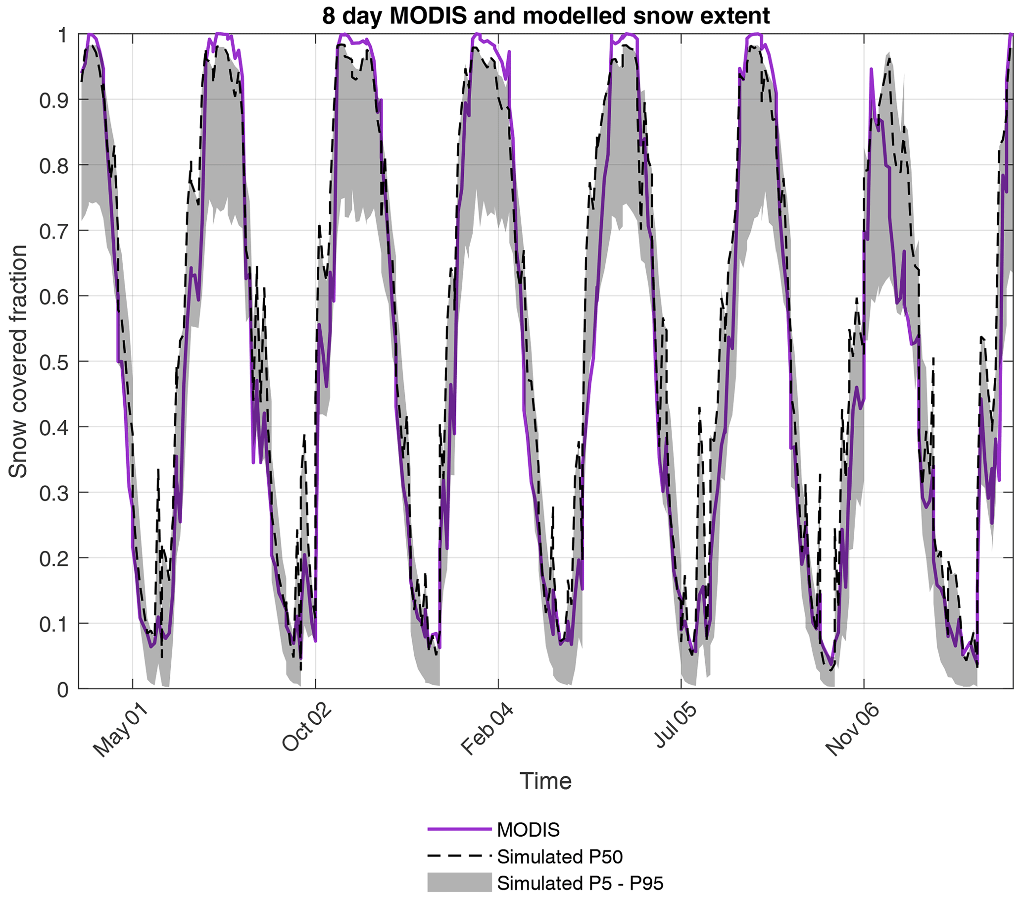
Figure 9MODIS and simulated weekly fraction of the basin covered in snow. The grey-shaded envelope shows the 5th–95th percentile range of the best 0.5 % calibration runs.
Table 6Seasonal validation metrics for MODIS and modelled snow extent for the 5th, median and 95th percentile prediction limits of the best 0.5 % calibration runs. Metrics for each season are calculated by averaging annual metrics over the years 2001–2007. Annual metrics are listed in Table S4.
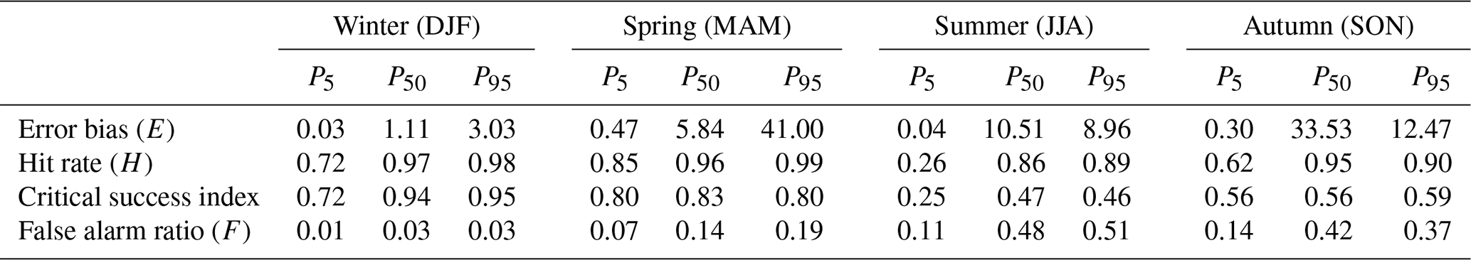
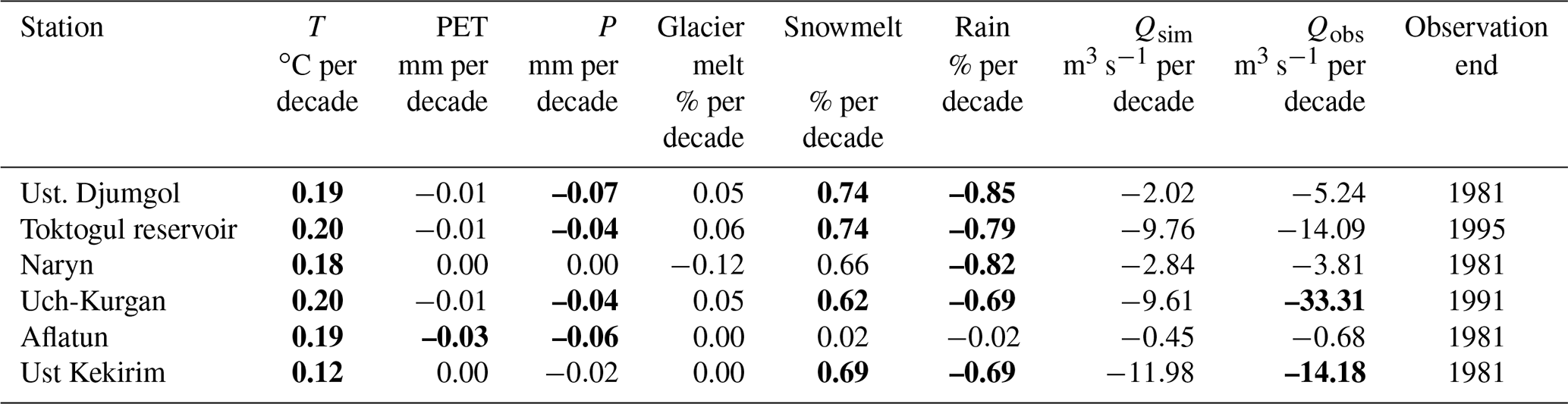
Table 7Trends in annual air temperature, PET and precipitation and the fraction of annual runoff from snowmelt, glacier melt and rainfall for the period 1951–2007. Trends are derived for the 50th percentile experiment using a Mann–Kendall test with Sen's slope estimator. Bold font indicates statistically significant trends with p values ≤ 0.05. Trends in annual simulated and observed discharge are also shown for the period 1951 to a variable end date which is dependent on the available observations.
3.10 Discharge components and timing
Adding the snow and glacier model to DECIPHeR makes it possible to disentangle the relative contributions of snow melting, glacier melting and rainfall to the total runoff and to determine the timing of when each component influences river flow. It is important to establish these present-day baseline conditions because these will change under future climate change scenarios. Figure 10 shows the percentage contribution of snow melting, glacier melting and rainfall to the total annual runoff averaged over the years 1951–2007. The discharge components are calculated using the 0.5 % best calibration parameters for the Uch-Kurgan station located at the outlet of the catchment. Snow melting is the largest contributor, consisting of 41 %–91 %, followed by the rain component (8 %–43 %) and the glacier component (0 %–15 %), where the ranges represent the 5th–95th percentile simulations across all the gauging stations. The glacier melt contribution is largest for the Naryn sub-catchment, comprising 4 %–15 % of the annual discharge. This is the headwater sub-catchment located in the Tien Shan mountains and has the largest glaciated area. In contrast, the glacier melting contribution at Aflatun is zero because this sub-catchment contains no glaciers. Figure 10 shows that the rainfall component is larger at the 95th percentile simulations than at the 5th and 50th percentile simulations. This is because the lapse rate at the 95th percentile simulations is higher (22 % 100 m−1) than at the 5th (1 % 100 m−1) and 50th (6 % 100 m−1) percentile simulations.
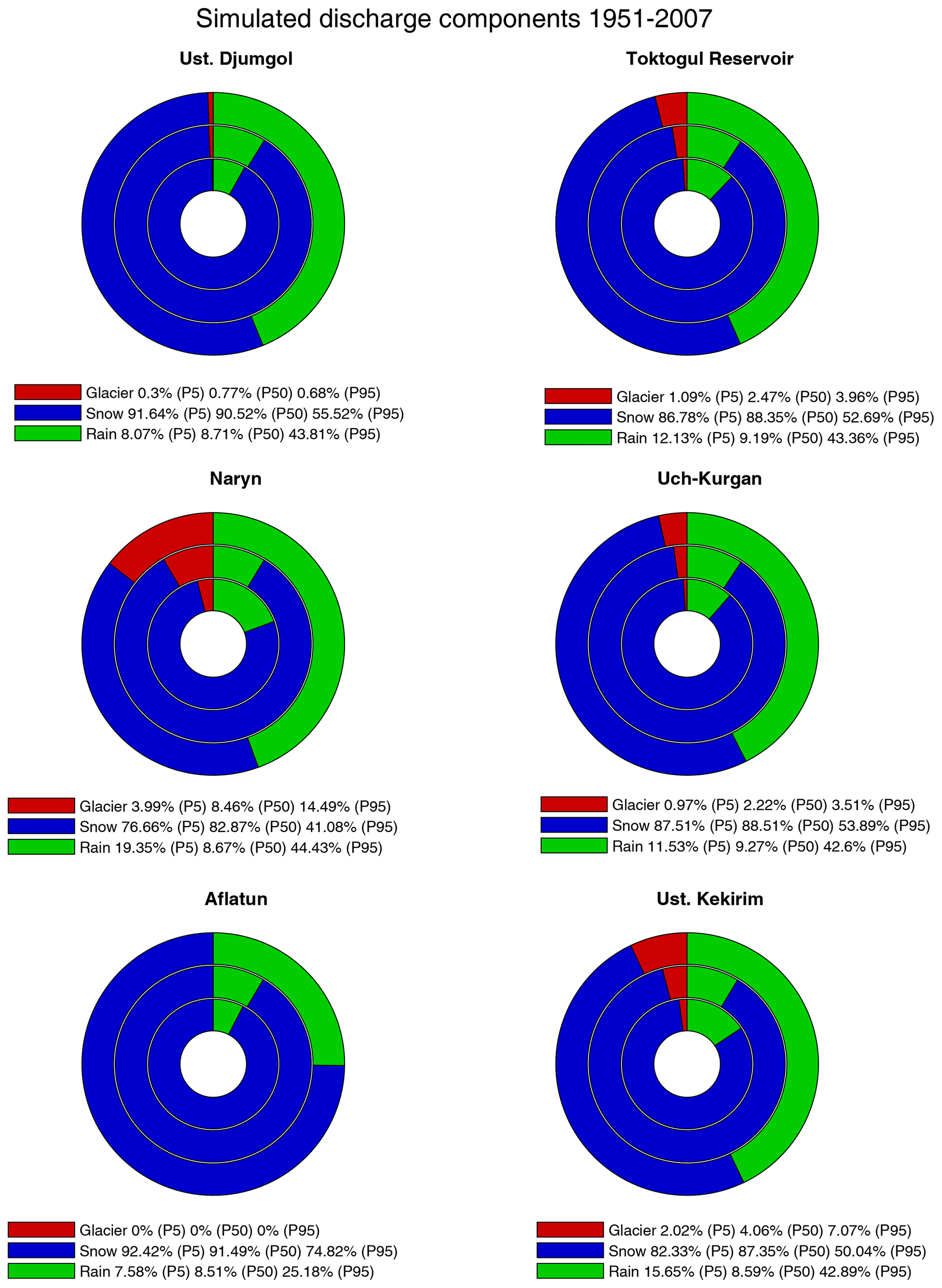
Figure 10Simulated fraction of annual runoff from snow melting, glacier melting and rain averaged for the years 1951–2007. The inner ring shows the 5th percentile, the middle ring is the 50th percentile and the outer ring is the 95th percentile simulation.
To determine whether there have been any statistically significant changes in the simulated discharge components since 1951, we do a trend detection analysis using a Mann–Kendall test and Sen's slope estimator with a significance level of 5 % on the 50th percentile discharge predictions (black line in Fig. 11). A trend detection is also run on the annual mean air temperature, potential evapotranspiration, precipitation and observed annual mean discharge. The trends are listed in Table 7. Despite a warming of 0.12–0.2∘ per decade, we only see a statistically significant trend in the observed discharge at Uch-Kurgan which is affected by the management of the Toktogul reservoir and at Ust Kekirim. There are no statistically significant trends in the glacier melt fraction and only small positive trends in the snowmelt and negative trends in the rainfall fractions of less than 1 % per decade at some of the gauging stations. The glacier melt and snowmelt fractions exhibit an anti-correlation which happens because the glacier melting occurs when the snowpack is depleted and the ice is exposed (Fig. 11).

Figure 11Annual percentage contribution of rain (green), snowmelt (blue) and glacier melt (red) to the total runoff for the period 1951–2007. The coloured envelopes show the 10 %-interval increasing percentile limits and the 50th percentile lines are shown in black.
Monthly hydrographs averaged over the period 1951–2007 show that discharge from snow melting peaks in the spring (April and May) (Fig. 12). Peak discharge from glacier melting happens later during the summer (June, July, August and September) after the snowpack has melted and glacier surfaces are exposed. This seasonal signal is seen at all the gauging stations except for Aflatun, where there are no glaciers. The glacier melt contribution is very high in August, where the upper range is 66 % for the Naryn sub-catchment and 41 % for Ust Kekirim. The percentage contributions of snowmelt, glacier melt and precipitation to the monthly runoff are listed in Table S4.
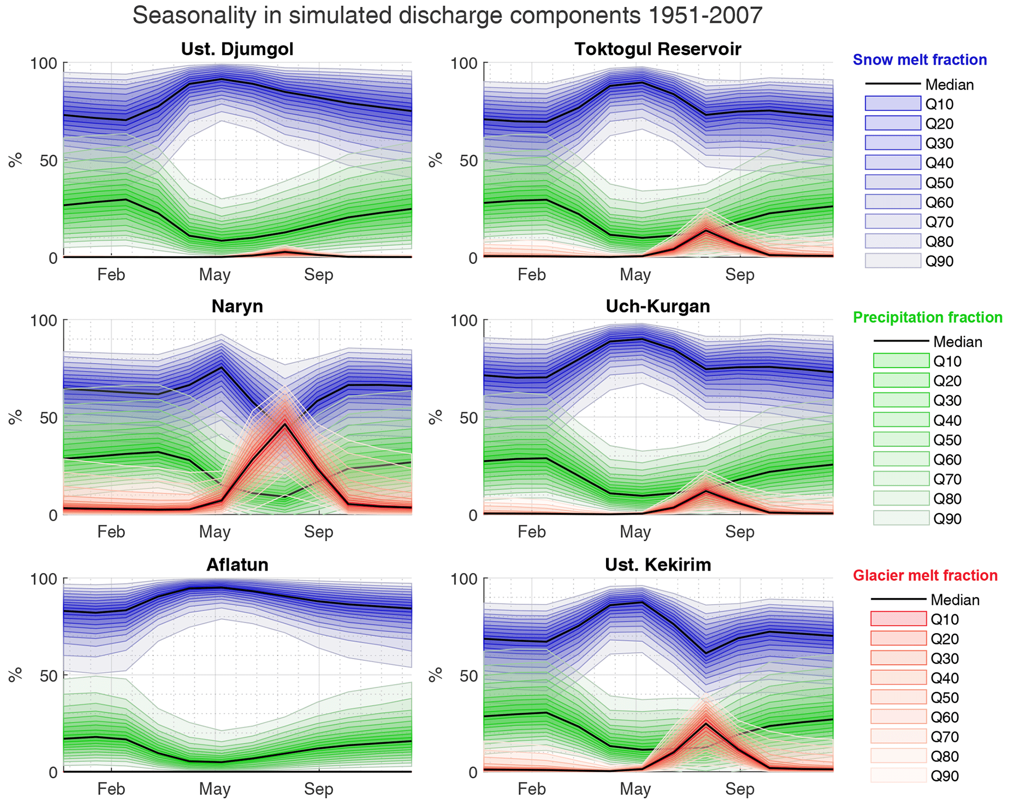
Figure 12Monthly simulated runoff components averaged over the period 1951–2007 for the top 0.5 % calibration simulations (n=751). The coloured envelope shows the 5th–95th percentile ranges.
In this paper we added a snowmelt and glacier melt model to the DECIPHeR hydrological model and demonstrated that the model performs well in predicting discharge and the spatial distribution of snow cover when compared to MODIS-observed snow extent. This updated version of the DECIPHeR model is suitable for simulating discharge in large glacier and snow-fed catchments at a high spatial resolution whilst maintaining the ability to include model uncertainty in the simulated discharge. Snow and glacier melting is modelled using the degree day approach, which requires only air temperature as an additional forcing input.
We used the model to calculate the relative contributions of snow, rain and glacier melt to the annual runoff. We found spatial variability in the relative contributions of each of the components. For the entire catchment (gauging station at Uch-Kurgan) the 50th percentile contributions are snow (89 %), rain (9 %) and glacier melting (2 %). These estimates are broadly consistent with Armstrong et al. (2019) who used MODIS imagery and degree day melt modelling to partition the runoff components in the Syr Darya River. Armstrong et al. (2019) found the runoff comprised of snow (74 %), rain (23 %) and glacier melting (2 %). Our estimates are slightly higher for the snowmelt contribution; however, our study focuses on the upper reaches of the Syr Darya River where the snowmelt is more likely to dominate the discharge.
Snow melting is the dominate component of the runoff at the six gauging stations. Throughout the Tien Shan long-term hydrological records of the former USSR show that snowmelt is the dominant source of runoff (Aizen et al., 1995). Further upstream in the Naryn sub-catchment the glacial melt contribution to the annual discharge is higher (4 %–15 %) than at Uch-Kurgan. Our upper estimate (15 %) is slightly lower than a study by Saks et al. (2022) who calculated that 23 % of the runoff originates from glacier melting in upper Naryn River. A possible explanation for why our estimate is lower is that our simulation period starts 30 years earlier (1951) than the study by Saks et al. (2022) which started in 1981.
In this study we set the behavioural models to the best 0.5 % simulations in the ensemble. This is an unconventional way of selecting behavioural models; however, it was important in our analysis to rank models according to their ability to capture seasonal discharge, particularly from spring snowmelt and summer glacier melt. Often behavioural models are selected using threshold values for guideline metrics. These metrics are calculated over the complete discharge time series, rather than for individual seasons. For example, metrics from Moriasi et al. (2007) are commonly used in the literature to categorize “acceptable”, “good” or “very good” simulations based on threshold values for NSE, PBIAS and RSR. Metrics calculated over the complete discharge time series are not a strong test of the model's ability to predict seasonal discharge. To our knowledge, there are no standardized guideline thresholds in the literature for seasonal metrics, therefore we selected the best 0.5 % of the ensemble. If we decided to define the behavioural models using a threshold for the seasonal RSR, then this would also be based on an arbitrary choice of value. A high threshold for seasonal RSR would be required to categorize the behavioural models because the summer values are high (see RSRJJA in Table 4).
We explored the impact of selecting alternative threshold values (1 %, 2.5 %, 5 % and 10 %) on the calibrated NSE values (Fig. S24). To obtain NSE values > 0.7 at all the gauging stations requires a threshold smaller than 1 %. This is notable at the Alfatun station, where the NSE value at the 0.5 % threshold is 0.74 but reduces to 0.63 at the 1 % threshold (95th percentile limit values). Figure S24 also shows how the uncertainty in the NSE values increases for higher threshold values. At the 10 % threshold the uncertainties in the NSE values are much larger than at the 0.5 % threshold.
In the Naryn sub-catchment which is the most upstream catchment located at elevations predominately exceeding 3000 m, the model performed best when the Esub parameter values are high. Esub reduces PET over snow and ice surfaces. This suggests that to improve the model at high elevations an orographic adjustment for PET is required. Currently the model uses surface values for PET; however, in practice PET decreases with elevation because of temperature cooling with height. Future work would calculate PET at the HRU level using an empirically derived relationship with temperature (Xie and Wang, 2020; Oudin et al., 2005). This type of parameterization would use the lapse rate adjusted HRU temperature calculated in the model. Alternatively, PET could be calculated using the Penman–Monteith (PM) method recommended by the Food and Agriculture Organization (Allen et al., 1998). This would require additional inputs such as solar radiation, wind speed and humidity. Nevertheless, the Penman–Monteith approach could potentially be more appropriate for high mountainous regions if the orographic increase in wind speed is also included.
Our simulated discharge and glaciated areas are presented with uncertainty bounds because many processes in the model are represented in a simplified way leading to uncertainty in the predictions. Likewise, forcing data in mountainous regions are often very sparse. We can see for example that the location of the gauging stations, used to derive the APHRODITE precipitation, are sparsely located and not homogeneously distributed across the catchment (see Fig. S19l). This leads to the requirement to calibrate snowfall and rainfall correction factors as they may vary across the catchment.
We found that, when calibrating the discharge, the RSR values were higher in the summer than during the other seasons, suggesting that improvements to the glacier model may improve the simulated summer discharge. One of the key missing processes is the role of permafrost which affects the upper part of the Naryn catchment. Barandun et al. (2020) showed that permafrost is the western Tien Shan is continuous above 3800 m, discontinuous between 3800 and 3600 m and sporadic between 3600 and 3000 m, and this can influence the runoff regime in three different ways. Firstly, the impermeable (or partially) frozen surface acts as a barrier over which water flows and this increases the speed of the runoff from snow and ice melting during the spring and summer. Secondly, every summer the thawing of ice-rich permafrost releases water that contributes to the streamflow. Thirdly, the degradation of ice-rich permafrost due to climate warming releases additional water. Permafrost responds more slowly to climate change than snow and glacier ice due to the insulating effect of the overlying land layer. This hidden water source could provide a buffer to water loss from glacier and snow melting.
We see from the comparison with MODIS data that snow extent is overpredicted in autumn, as evidenced by a higher false alarm ratio. This may explain why the catchment-wide glaciated area predicted by the model is higher than the Landsat observation at the end of the simulation period (median value in Fig. 6 is 988 km2 and observation is 926±23 % km2). It is open to question whether the overestimate in snow extent is caused by an overestimate in accumulation or an underestimate in melting. The simple degree day melt model does not account for all the complex processes that contribute to melting. Terrain aspect can have a large impact on the quantity of solar energy available for melting. Snow and glaciers on south-facing slopes receive more sunlight than north facing slopes in the Northern Hemisphere. The effect of aspect could be included by modifying the degree day factor as a function of the slope (Immerzeel et al., 2012, 2013). Another improvement to the melt scheme would involve calibrating the temperature thresholds for glacier and snow melting. Currently the threshold temperatures for melting ice and snow are set to 0∘. Alternative methods to calculate melting, such as using an enhanced temperature index model or full energy balance in scheme may help to improve the predictions of snow extent in the autumn.
Future versions of the model could also consider the impact of debris cover on glacier surfaces and its effect on glacier melt. While thin debris layers decrease albedo and enhance local melt rates, once the debris layer exceeds a few centimeters, it insulates the glacier which reduces melt rates (Fyffe et al., 2019). In addition, some debris-covered glaciers in High Mountain Asia and elsewhere undergo a transition to form rock glaciers; these contain large ice volumes and appear to be more resilient to warming than ice glaciers (Jones et al., 2021). As a result, the degree day melt and temperature lag factors could be modified in regions where debris-covered glaciers and rock glaciers are present. Information on the present-day distribution of debris-covered glaciers derived from remote sensing is available to implement this (Herreid and Pellicciotti, 2020; Scherler et al., 2018). However, similar information on rock glaciers is not yet available, and the climate and hydrological response of rock glaciers differs from that of debris-covered glaciers.
Additional developments would improve the representation of water flow through the ice and snow. Currently, when rain falls on a HRU, the water goes straight to the root zone, so we do not consider the percolation of water through the ice and snow. This would require a more complex model that includes the density and pore space of the snowpack and ice. We have not included the re-freezing of meltwater, which would increase the snowpack or ice depth, nor have we included the process by which rainfall adds warmth to the snowpack or ice, which enhances melting.
Glacier flow has not been included in the model. To estimate a catchment-wide glaciated area, an arbitrary threshold of 1 mm is used to identify the presence of ice. Figure S20 shows the impact of using alternative thresholds of m, 1 cm and 1 m. We see that the catchment-wide glaciated area is sensitive to the choice of threshold value. Including ice flow and constraining this using mass balance observations in the calibration procedure would enable us to select a realistic threshold over an arbitrary one.
Glacier ice is not allowed to advance beyond the perimeter of the initial glacier outlines, meaning that the model is unsuitable for applications where glaciers are surging. Globally, glaciers have been in a state of retreat (Zemp et al., 2019); however, this has not been the case in the Pamir–Karakorum region, where observations show that glaciers have advanced (Hewitt, 2005; Gardelle et al., 2012, 2013). Nevertheless, a more recent study by Hugonnet et al. (2021) shows that this anomalous mass gain appears to have ended. It is reasonable to assume that glaciers will only retreat for applications where the model is driven by future climate scenarios.
A future study would explore the sensitivity of the model to the initial glacier and snow conditions. Glacier ice is initialized with a fixed temperature of −5 ∘C and snow temperature was set to 0 ∘C. The GlabTop2 method (Frey et al., 2014) used to calculate the initial glacier thickness contains uncertainty due to empirically derived parameterization to estimate basal shear stress. A sensitivity study would test alternative parameterizations or explore other methods. For example, the Volume and Topography Automation (VOLTA) model (Gharehchahi et al., 2020), which includes the effect of side drag on glacier thicknesses, could be used.
The model does not include snow redistribution by wind and avalanches, so multi‐year accumulation of snow at high elevations leads to the well-known problem of isolated “snow towers”. Disregarding snow redistribution in models can not only lead to the formation of these “snow towers”, but can also have an impact on the timing and magnitude of the snowmelt runoff (Freudiger et al., 2017). At the end of the simulations in 2007, 55 of the total 61 481 HRUs have daily snow depths exceeding 100 m. This might eventually have a significant impact on river discharge if the model were run over longer simulation periods. “Snow towers” were found predominately in a small region located in the western part of the catchment. This can be seen in Fig. S21 showing snow depths and Fig. S22 showing a snow tower.
Future work should focus on improving the calibration method to include additional observations. In this study, it was not possible to include glacier mass balance observations in the calibration because of the lack of historical observations during the period 1951–1970. The large range of glaciated areas predicted by the model at the end of the simulation period in 2007 shows that the model can make good predictions in discharge (Fig. 5) whilst simultaneously predicting a large range of estimates for glacier area (Fig. 6). This highlights the importance of including ancillary observations, such as glacier mass balance, snow depth or snow extent, in the calibration to help constrain the predictions. Currently, the model performance is not sensitive to many of the calibration parameter values (Fig. S15). It is possible that some parameter combinations compensate for each other. For example, a high snowfall correction factor may be compensated for by a lower precipitation lapse rate. More analysis needs to be conducted on the sensitivity of the new snow and ice parameters added to DECIPHeR as part of this study, both in time and space, and the types of data that may help to constrain these parameters. Remote sensing snow products have been used to calibrate models, and studies indicated that the integration of data such as MODIS snow cover into hydrological models can improve the simulated snow cover whilst maintaining model performance with respect to runoff (Parajka and Bloschl, 2008). For example, Hong et al. (2015) integrated glacier annual mass balance observations in the calibration of a glacio-hydrological model to simulate discharge for catchments in Norway and the Himalaya. Glacier mass balance was considered so relevant that an annual mass balance observation was given a weighting of 10 000 times more than a discharge observation.
We have not included the impact of water abstraction for irrigation or water storage from reservoirs in the model. The results show that a reservoir model is required to improve estimates of discharge at the Uch-Kurgan station. Our assumption is that water abstraction for irrigation is minimal compared to natural streamflow. This assumption is supported by observations of flow intake at irrigation channels, which is very small compared to the flow measured at the gauging stations. Observations of monthly flow intake for the major irrigation channels in Kyrgyzstan are archived in the Central Asian Waterinfo Database. Three channels are located in the Naryn basin: Kulanak, Aryk Chegirtke and Alfatun. (See Fig. S1 for the locations of these irrigation head intakes.) The Kulanak channel is the longest (40 km) and irrigates an area of 45 km2 in the Kulanak Valley. The maximum monthly flow intake at the head of the channel is approximately 3.6 m3 s−1 (Fig. S22), which is significantly lower than the peak flow observed at the Ust Kekirim and Naryn stations. Nonetheless, excluding the impact of irrigation will result in a small uncertainty in the prediction of the snowmelt and glacier melt contributions to streamflow because the majority of the water abstraction takes place during in spring and summer (April to August).
The model evaluation presented here is an essential prerequisite for running future simulations to predict how river flow will change as glaciers lose mass and the seasonal snowpack disappears. We showed that for the period 1951–2007 discharge increases in the spring (April–May) when the snowpack melts and peaks in the summer (June, July, August and September) when glacier melting commences. Under future climate change scenarios we may expect the timing of the peak snowmelt and glacier melt contributions to happen sooner in the year (Gan et al., 2015). These changes will have implications for water supply in the Ferghana Valley and downstream in the Syr Darya River.
In this study we implemented a degree day snowmelt and glacier melt model in the DECIPHeR model. The motivation for this work was to develop a hydrological model that can be used to simulate discharge in very large glaciated and snow-fed catchments, at a high spatial resolution, whilst maintaining the ability to explore model uncertainty. The overarching aim is to develop a tool for predicting changes in river flow under future climate change scenarios.
We describe the snow and glacier model and its application to the Naryn River catchment, central Asia. The model is evaluated using discharge observations, MODIS snow extent and catchment-wide glaciated area derived from Landsat observations. The model is found to be robust at predicting monthly discharge at six gauging stations over the period 1951 to the variable end date between 1980 and 1995 depending on the availability of discharge observations. The validation with MODIS snow extent shows that the model can reproduce the spatial extent in seasonal snow cover reasonably well in winter, summer and spring, with mean hit rates exceeding 0.86 (median ensemble member of the best 0.5 % calibration simulations), but overestimates snow extent in autumn as reflected by a high false alarm ratio and a positive bias. The best 0.5 % calibration simulations using six different and equally weighted metrics reproduce a catchment-wide glaciated area consistent with Landsat observations in the late 1990s and mid-2000s. There is, however, a large range of glaciated area estimates within this ensemble. This means that good predictions of discharge can be made concurrently with a large range of glacier area estimates. This strengthens the case that, to make robust predictions, additional observations such as glacier mass balance, snow depth or snow extent should be included in the model calibration.
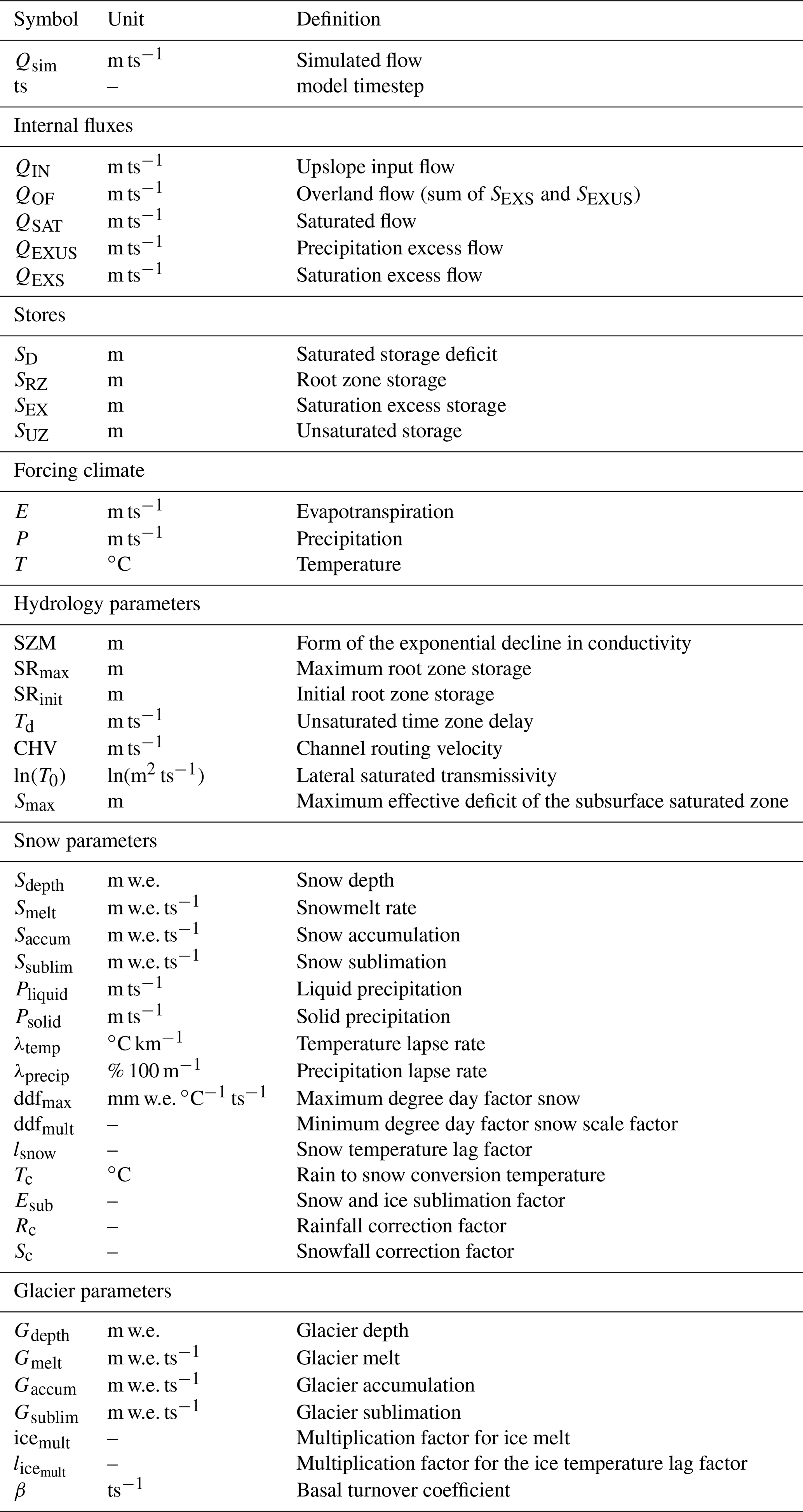
The following model forcing and evaluation datasets are publicly available. The ERA5 reanalysis data (Copernicus) are available from the Copernicus Climate Data Store (https://doi.org/10.24381/cds.adbb2d47; CDS, 2001). The APHRODITE precipitation (Yatagai et al., 2012) can be downloaded from http://aphrodite.st.hirosaki-u.ac.jp/download (APHRODITE, 2021). Monthly discharge observations are available from the GRDC data portal at https://portal.grdc.bafg.de (GRDC, 2018). The MERIT DEM (Yamazaki et al., 2017) is available at http://hydro.iis.u-tokyo.ac.jp/~yamadai/MERIT_DEM (Hydro, 2018). The MODIS 500 m resolution 8 d snow cover extent MOD10A2 version 6 (Hall and Riggs, 2016) is available from https://doi.org/10.5067/MODIS/MOD10A2.006. Landsat glacier outlines (Kriegel et al., 2013) can be accessed by contacting the authors.
The DECIPHeR model code is freely available under the terms of the GNU General Public License version 3.0. The model code is written in FORTRAN 90 and can be downloaded from the Zenodo repository at https://doi.org/10.5281/zenodo.7544529 (Shannon, 2023).
The supplement related to this article is available online at: https://doi.org/10.5194/hess-27-453-2023-supplement.
The paper was prepared by SSh with contributions from all the co-authors. SSh wrote the snow and glacier models with contributions from GC and MK. SSh generated the model output and performed the analysis. JF, TP, GC, MK and SH assisted with the experimental design, analysis and interpretation of results. DK provided the Landsat glacier outlines.
The contact author has declared that none of the authors has any competing interests.
Publisher's note: Copernicus Publications remains neutral with regard to jurisdictional claims in published maps and institutional affiliations.
This article is part of the special issue “Hydrological response to climatic and cryospheric changes in high-mountain regions”. It is not associated with a conference.
This work was carried out using the computational facilities of the Advanced Computing Research Centre at the University of Bristol. The work was funded by the Leverhulme Trust Research Project grant reference RPG-2017-083. Jim Freer was partly supported for his time on this paper by the Global Water Futures program.
This research has been supported by the Leverhulme Trust (grant no. RPG-2017-083).
This paper was edited by Wouter Buytaert and reviewed by Jonathan D. Mackay and one anonymous referee.
Aizen, V. B., Aizen, E. M., and Melack, J. M.: Climate, Snow Cover, Glaciers, and Runoff in the Tien Shan, central Asia, Am. J. Water Resour. Assoc., 31, 1113001129, https://doi.org/10.1111/j.1752-1688.1995.tb03426.x, 1995. a
Allen, R., Pereira, L., Raes, D., and Smith, M.: Crop evapotranspiration – Guidelines for computing crop water requirements, FAO Irrigation and drainage paper 56, Fao, Rome, https://www.fao.org/3/X0490E/X0490E00.htm (last access: 19 January 2023), 1998. a
Ambroise, B., Freer, J., and Beven, K.: Application of a generalized TOPMODEL to the small Ringelbach catchment, Vosges, France, Water Resour. Res., 32, 2147–2159, https://doi.org/10.1029/95WR03715, 1996. a
APHRODITE: APHRODITE's Water Resources, http://aphrodite.st.hirosaki-u.ac.jp/download, last access: 5 May 2021. a
Armstrong, R. L., Rittger, K., Brodzik, M. J., Racoviteanu, A., Barrett, A. P., Khalsa, S. J. S., Raup, B., Hill, A. F., Khan, A. L., Wilson, A. M., Kayastha, R. B., Fetterer, F., and Armstrong, B.: Runoff from glacier ice and seasonal snow in High Asia: separating melt water sources in river flow, Reg. Environ. Change, 19, 1249–1261, https://doi.org/10.1007/s10113-018-1429-0, 2019. a, b, c
Barandun, M., Fiddes, J., Scherler, M., Mathys, T., Saks, T., Petrakov, D., and Hoelzle, M.: The state and future of the cryosphere in Central Asia, Water Secur., 11, 100072, https://doi.org/10.1016/j.wasec.2020.100072, 2020. a, b
Bernauer, T. and Siegfried, T.: Climate change and international water conflict in Central Asia, J. Peace Res., 49, 227–239, https://doi.org/10.1177/0022343311425843, 2012. a
Beven, K.: A manifesto for the equifinality thesis, J. Hydrol., 320, 18–36, https://doi.org/10.1016/j.jhydrol.2005.07.007, 2006. a
Beven, K. and Binley, A.: The Future Of Distributed Models – Model Calibration And Uncertainty Prediction, Hydrol. Process., 6, 279–298, https://doi.org/10.1002/hyp.3360060305, 1992. a
Beven, K. and Freer, J.: A dynamic TOPMODEL, Hydrol. Process., 15, 1993–2011, https://doi.org/10.1002/hyp.252, 2001. a
CDS: ERA5 hourly data on single levels from 1959 to present, https://doi.org/10.24381/cds.adbb2d47, last access: 5 February 2021. a
Chen, Y. N., Li, W. H., Deng, H. J., Fang, G. H., and Li, Z.: Changes in Central Asia's Water Tower: Past, Present and Future, Scient. Rep., 6, 35458, https://doi.org/10.1038/srep39364, 2016. a
Copernicus: ERA5: Fifth generation of ECMWF atmospheric reanalyses of the global climate, Copernicus Climate Change Service Climate Data Store (CDS), https://cds.climate.copernicus.eu (last access: 5 February 2021), 2017. a
Coxon, G., Freer, J., Lane, R., Dunne, T., Knoben, W. J. M., Howden, N. J. K., Quinn, N., Wagener, T., and Woods, R.: DECIPHeR v1: Dynamic fluxEs and ConnectIvity for Predictions of HydRology, Geosci. Model Dev., 12, 2285–2306, https://doi.org/10.5194/gmd-12-2285-2019, 2019. a, b, c, d, e, f, g, h, i, j
Duethmann, D., Peters, J., Blume, T., Vorogushyn, S., and Guentner, A.: The value of satellite- derived snow cover images for calibrating a hydrological model in snow- dominated catchments in Central Asia, Water Resour. Res., 50, 2002–2021, https://doi.org/10.1002/2013WR014382, 2014. a
Engel, Z., Šobr, M., and Yerokhin, S. A.: Changes of Petrov glacier and its proglacial lake in the Akshiirak massif, central Tien Shan, since 1977, J. Glaciol., 58, 388–398, https://doi.org/10.3189/2012JoG11J085, 2012. a
Farinotti, D., Usselmann, S., Huss, M., Bauder, A., and Funk, M.: Runoff evolution in the Swiss Alps: projections for selected high-alpine catchments based on ENSEMBLES scenarios, Hydrol. Process., 26, 1909–1924, https://doi.org/10.1002/hyp.8276, 2012. a
Finger, D., Pellicciotti, F., Konz, M., Rimkus, S., and Burlando, P.: The value of glacier mass balance, satellite snow cover images, and hourly discharge for improving the performance of a physically based distributed hydrological model, Water Resour. Res., 47, W07519, https://doi.org/10.1029/2010WR009824, 2011. a
Finger, D., Vis, M., Huss, M., and Seibert, J.: The value of multiple data set calibration versus model complexity for improving the performance of hydrological models in mountain catchments, Water Resour. Res., 51, 1939–1958, https://doi.org/10.1002/2014WR015712, 2015. a
Fontaine, T., Cruickshank, T., Arnold, J., and Hotchkiss, R.: Development of a snowfall-snowmelt routine for mountainous terrain for the soil water assessment tool (SWAT), J. Hydrol., 262, 209–223, https://doi.org/10.1016/S0022-1694(02)00029-X, 2002. a
Frans, C., Istanbulluoglu, E., Lettenmaier, D. P., Fountain, A. G., and Riedel, J.: Glacier Recession and the Response of Summer Streamflow in the Pacific Northwest United States, 1960–2099, Water Resour. Res., 54, 6202–6225, https://doi.org/10.1029/2017WR021764, 2018. a
Freer, J., Beven, K., and Ambroise, B.: Bayesian estimation of uncertainty in runoff prediction and the value of data: An application of the GLUE approach, Water Resour. Res., 32, 2161–2173, https://doi.org/10.1029/95wr03723, 1996. a
Freer, J., McMillan, H., McDonnell, J., and Beven, K.: Constraining dynamic TOPMODEL responses for imprecise water table information using fuzzy rule based performance measures, J. Hydrol., 291, 254–277, https://doi.org/10.1016/j.jhydrol.2003.12.037, 2004. a
Freudiger, D., Kohn, I., Seibert, J., Stahl, K., and Weiler, M.: Snow redistribution for the hydrological modeling of alpine catchments, Wiley Interdisciplin. Rev.-Water, 4, e1232, https://doi.org/10.1002/wat2.1232, 2017. a
Frey, H., Machguth, H., Huss, M., Huggel, C., Bajracharya, S., Bolch, T., Kulkarni, A., Linsbauer, A., Salzmann, N., and Stoffel, M.: Estimating the volume of glaciers in the Himalayan–Karakoram region using different methods, The Cryosphere, 8, 2313–2333, https://doi.org/10.5194/tc-8-2313-2014, 2014. a, b
Fyffe, C., Brock, B., Kirkbride, M., Mair, D., Arnold, N., Smiraglia, C., Diolaiuti, G., and Diotri, F.: Do debris-covered glaciers demonstrate distinctive hydrological behaviour compared to clean glaciers?, J. Hydrol., 570, 584–597, https://doi.org/10.1016/j.jhydrol.2018.12.069, 2019. a
Gan, R., Luo, Y., Zuo, Q. T., and Sun, L.: Effects of projected climate change on the glacier and runoff generation in the Naryn River Basin, Central Asia, J. Hydrol., 523, 240–251, https://doi.org/10.1016/j.jhydrol.2015.01.057, 2015. a
Gardelle, J., Berthier, E., and Arnaud, Y.: Slight mass gain of Karakoram glaciers in the early twenty-first century, Nat. Geosci., 5, 322–325, https://doi.org/10.1038/ngeo1450, 2012. a
Gardelle, J., Berthier, E., Arnaud, Y., and Kaab, A.: Region-wide glacier mass balances over the Pamir-Karakoram-Himalaya during 1999–2011, The Cryosphere, 7, 1263–1286, https://doi.org/10.5194/tc-7-1263-2013, 2013. a
Gharehchahi, S., James, W. H. M., Bhardwaj, A., Jensen, J. L. R., Sam, L., Ballinger, T. J., and Butler, D. R.: Glacier Ice Thickness Estimation and Future Lake Formation in Swiss Southwestern Alps – The Upper Rhone Catchment: A VOLTA Application, Rem. Sens., 12, 22, https://doi.org/10.3390/rs12223709, 2020. a
GRDC: Data Download, https://portal.grdc.bafg.de, last access: 14 September 2018. a
Hagg, W., Mayer, C., Lambrecht, A., Kriegel, D., and Azizov, E.: Glacier changes in the Big Naryn basin, Central Tian Shan, Global Planet. Change, 110, 40–50, https://doi.org/10.1016/j.gloplacha.2012.07.010, 2013. a
Hall, D. K. and Riggs, G. A.: MODIS/Terra Snow Cover 8-Day L3 Global 500 m SIN Grid, Version 6, NSIDC [data set], https://doi.org/10.5067/MODIS/MOD10A2.006, 2016. a, b
Herreid, S. and Pellicciotti, F.: The state of rock debris covering Earth's glaciers, Nat. Geosci., 13, 621–627, https://doi.org/10.1038/s41561-020-0615-0, 2020. a
Hewitt, K.: The Karakoram anomaly? Glacier expansion and the `elevation effect', Karakoram Himalaya, Mt. Res. Dev., 25, 332–340, https://doi.org/10.1659/0276-4741(2005)025[0332:tkagea]2.0.co;2, 2005. a
Hong, L., Stein, B., Xu, C.-Y., Huss, M., Kjetil, M., and Jain, S. K.: Integrating a glacier retreat model into a hydrological model – Case studies of three glacierised catchments in Norway and Himalayan region, J. Hydrol. 527, 656–667, https://doi.org/10.1016/j.jhydrol.2015.05.017, 2015. a
Horton, P., Schaefli, B., and Kauzlaric, M.: Why do we have so many different hydrological models? A review based on the case of Switzerland, WIREs Water, 9, e1574, https://doi.org/10.1002/wat2.1574, 2022. a
Hugonnet, R., McNabb, R., Berthier, E., Menounos, B., Nuth, C., Girod, L., Farinotti, D., Huss, M., Dussaillant, I., Brun, F., and Kaab, A.: Accelerated global glacier mass loss in the early twenty-first century, Nature, 592, 726–731, https://doi.org/10.1038/s41586-021-03436-z, 2021. a
Hydro: MERIT DEM: Multi-Error-Removed Improved-Terrain DEM, http://hydro.iis.u-tokyo.ac.jp/~yamadai/MERIT_DEM, last access: 7 March 2018. a
Immerzeel, W. W., van Beek, L. P. H., and Bierkens, M. F. P.: Climate Change Will Affect the Asian Water Towers, Science, 328, 1382–1385, https://doi.org/10.1126/science.1183188, 2010. a
Immerzeel, W. W., van Beek, L. P. H., Konz, M., Shrestha, A. B., and Bierkens, M. F. P.: Hydrological response to climate change in a glacierized catchment in the Himalayas, Climatic Change, 110, 721–736, https://doi.org/10.1007/s10584-011-0143-4, 2012. a
Immerzeel, W. W., Pellicciotti, F., and Bierkens, M. F. P.: Rising river flows throughout the twenty-first century in two Himalayan glacierized watersheds, Nat. Geosci., 3, 742–745, https://doi.org/10.1038/ngeo1896, 2013. a, b
Immerzeel, W. W., Lutz, A. F., Andrade, M., Bahl, A., Biemans, H., Bolch, T., Hyde, S., Brumby, S., Davies, B. J., Elmore, A. C., Emmer, A., Feng, M., Fernandez, A., Haritashya, U., Kargel, J. S., Koppes, M., Kraaijenbrink, P. D. A., Kulkarni, A. V., Mayewski, P. A., Nepal, S., Pacheco, P., Painter, T. H., Pellicciotti, F., Rajaram, H., Rupper, S., Sinisalo, A., Shrestha, A. B., Viviroli, D., Wada, Y., Xiao, C., Yao, T., and Baillie, J. E. M.: Importance and vulnerability of the world's water towers, Nature, 577, 364–369, https://doi.org/10.1038/s41586-019-1822-y, 2020. a
Janský, B., Šobr, M., and Engel, Z.: Outburst flood hazard: Case studies from the Tien-Shan Mountains, Kyrgyzstan, Limnologica, 40, 358–364, https://doi.org/10.1016/j.limno.2009.11.013, 2010. a
Jones, D., Harrison, S., Anderson, K., Shannon, S., and Betts, R.: Rock glaciers represent hidden water stores in the Himalaya, Sci. Total Environ., 793, 145368, https://doi.org/10.1016/j.scitotenv.2021.145368, 2021. a
Kaser, G., Großhauser, M., and Marzeion, B.: Contribution potential of glaciers to water availability in different climate regimes, P. Natl. Acad. Sci. USA, 107, 20223–20227, https://doi.org/10.1073/pnas.1008162107, 2010. a
Koboltschnig, G. R., Schöner, W., Zappa, M., Kroisleitner, C., and Holzmann, H.: Runoff modelling of the glacierized Alpine Upper Salzach basin (Austria): multi-criteria result validation, Hydrol. Process., 22, 3950–3964, https://doi.org/10.1002/hyp.7112, 2008. a
Kraaijenbrink, P. D. A., Bierkens, M. F. P., Lutz, A. F., and Immerzeel, W. W.: Impact of a global temperature rise of 1.5 degrees Celsius on Asia's glaciers, Nature, 549, 257–260, https://doi.org/10.1038/nature23878, 2017. a
Kriegel, D., Mayer, C., Hagg, W., Vorogushyn, S., Duethmann, D., Gafurov, A., and Farinotti, D.: Changes in glacierisation, climate and runoff in the second half of the 20th century in the Naryn basin, Central Asia, Global Planet. Change, 110, 51–61, https://doi.org/10.1016/j.gloplacha.2013.05.014, 2013. a, b, c, d, e, f
Lambert, L. and Chitrakar, B. D.: Variation of potential evapotranspiration with elevation in Nepal, Mt. Res. Dev., 9, 145–152–50, 1989. a
Lane, R. A., Freer, J. E., Coxon, G., and Wagener, T.: Incorporating Uncertainty Into Multiscale Parameter Regionalization to Evaluate the Performance of Nationally Consistent Parameter Fields for a Hydrological Model, Water Resour. Res., 57, 10, https://doi.org/10.1029/2020WR028393, 2021. a
Lindstrom, G., Johansson, B., Persson, M., Gardelin, M., and Bergstrom, S.: Development and test of the distributed HBV-96 hydrological model, J. Hydrol., 201, 272–288, https://doi.org/10.1016/S0022-1694(97)00041-3, 1997. a
Liu, Q. and Liu, S.: Response of glacier mass balance to climate change in the Tianshan Mountains during the second half of the twentieth century, Cllim. Dynam., 46, 303–316, https://doi.org/10.1007/s00382-015-2585-2, 2016. a
Luo, Y., Arnold, J., Liu, S. Y., Wang, X. Y., and Chen, X.: Inclusion of glacier processes for distributed hydrological modeling at basin scale with application to a watershed in Tianshan Mountains, northwest China, J. Hydrol., 477, 72–85, https://doi.org/10.1016/j.jhydrol.2012.11.005, 2013a. a
Luo, Y., Arnold, J., Liu, S. Y., Wang, X. Y., and Chen, X.: Inclusion of glacier processes for distributed hydrological modeling at basin scale with application to a watershed in Tianshan Mountains, northwest China, J. Hydrol., 477, 72–85, https://doi.org/10.1016/j.jhydrol.2012.11.005, 2013b. a
Lutz, A., Immerzeel, W. W., Shrestha, A. B., and Bierkens, M. F. P.: Consistent increase in High Asia's runoff due to increasing glacier melt and precipitation, Nat. Clim.Change, 4, 587–592, https://doi.org/10.1038/nclimate2237, 2014. a
Magnusson, J., Wever, N., Essery, R., Helbig, N., Winstral, A., and Jonas, T.: Evaluating snow models with varying process representations for hydrological applications, Water Resour. Res., 51, 2707–2723, https://doi.org/10.1002/2014WR016498, 2015. a
Malsy, M., Beek, T. A. D., and Florke, M.: Evaluation of large-scale precipitation data sets for water resources modelling in Central Asia, Environ. Earth Sci., 73, 787–799, https://doi.org/10.1007/s12665-014-3107-y, 2015. a
Marzeion, B., Hock, R., Anderson, B., Bliss, A., Champollion, N., Fujita, K., Huss, M., Immerzeel, W. W., Kraaijenbrink, P., Malles, J. H., Maussion, F., Radic, V., Rounce, D. R., Sakai, A., Shannon, S., van deWal, R., and Zekollari, H.: Partitioning the Uncertainty of Ensemble Projections of Global Glacier Mass Change, Earths Future, 8, e2019EF001470, https://doi.org/10.1029/2019ef001470, 2020. a
Mayr, E., Hagg, W., Mayer, C., and Braun, L.: Calibrating a spatially distributed conceptual hydrological model using runoff, annual mass balance and winter mass balance, J. Hydrol., 478, 40–49, https://doi.org/10.1016/j.jhydrol.2012.11.035, 2013. a, b
McKay, M. D., Beckman, R. J., and Conover, W. J.: Comparison of Three Methods for Selecting Values of Input Variables in the Analysis of Output from a Computer Code, Technometrics, 21, 239–245, 1979. a
Meier, J., Zabel, F., and Mauser, W.: A global approach to estimate irrigated areas – a comparison between different data and statistics, Hydrol. Earth Syst. Sci., 22, 1119–1133, https://doi.org/10.5194/hess-22-1119-2018, 2018. a
Metcalfe, P., Beven, K., and Freer, J.: Dynamic TOPMODEL: A new implementation in R and its sensitivity to time and space steps, Environ. Model. Softw., 72, 155–172, https://doi.org/10.1016/j.envsoft.2015.06.010, 2015. a
Moriasi, D. N., Arnold, J. G., Van Liew, M. W., Bingner, R. L., Harmel, R. D., and Veith, T. L.: Model evaluation guidelines for systematic quantification of accuracy in watershed simulations, T. ASABE, 50, 885–900, 2007. a, b
Neitsch, S. L., Arnold, J. G., Kiniry, J. R., and Williams, J. R.: Soil and Water Assessment Tool Theoretical Documentation, Version 2005, Grassland, Soil and Water Research Laboratory, http://swat.tamu.edu/documentation (last access: 30 January 2019), 2005. a
Omani, N., Srinivasan, R., Karthikeyan, R., and Smith, P. K.: Hydrological Modeling of Highly Glacierized Basins (Andes, Alps, and Central Asia), Water, 9, 11, https://doi.org/10.3390/w9020111, 2017. a, b
Oudin, L., Hervieu, F., Michel, C., Perrin, C., Andreassian, V., Anctil, F., and Loumagne, C.: Which potential evapotranspiration input for a lumped rainfall-runoff model? Part 2 – Towards a simple and efficient potential evapotranspiration model for rainfall-runoff modelling, J. Hydrol., 303, 290–306, https://doi.org/10.1016/j.jhydrol.2004.08.026, 2005. a
Parajka, J. and Bloschl, G.: The value of MODIS snow cover data in validating and calibrating conceptual hydrologic models, J. Hydrol., 358, 240–258, https://doi.org/10.1016/j.jhydrol.2008.06.006, 2008. a
Paterson, W.: The physics of glaciers, in: 3rd Edn., Pergamon Press, Oxford, New York, Tokyo, https://doi.org/10.1016/C2009-0-14802-X, 1994. a
Pellicciotti, F., Buergi, C., Immerzeel, W. W., Konz, M., and Shrestha, A. B.: Challenges and Uncertainties in Hydrological Modeling of Remote Hindu Kush-Karakoram-Himalayan (HKH) Basins: Suggestions for Calibration Strategies, Mt. Res. Dev., 32, 39–50, https://doi.org/10.1659/MRD-JOURNAL-D-11-00092.1, 2012. a
Peters, N., Freer, J., and Beven, K.: Modelling hydrologic responses in a small forested catchment (Panola Mountain, Georgia, USA): a comparison of the original and a new dynamic TOPMODEL, Hydrol. Process., 17, 345–362, https://doi.org/10.1002/hyp.1128, 2003. a
Pieczonka, T. and Bolch, T.: Region-wide glacier mass budgets and area changes for the Central Tien Shan between 1975 and 1999 using Hexagon KH-9 imagery, Global Planet. Change, 128, 1–13, https://doi.org/10.1016/j.gloplacha.2014.11.014, 2015. a
Pu, Z. X., Xu, L., and Salomonson, V. V.: MODIS/Terra observed seasonal variations of snow cover over the Tibetan Plateau, Geophys. Res. Lett., 34, L06706, https://doi.org/10.1029/2007gl029262, 2007. a
Radchenko, I., Dernedde, Y., Mannig, B., Frede, H.-G., and Breuer, L.: Climate Change Impacts on Runoff in the Ferghana Valley (Central Asia), Water Resour., 44, 707–730, https://doi.org/10.1134/S0097807817050098, 2017. a, b
Ragettli, S. and Pellicciotti, F.: Calibration of a physically based, spatially distributed hydrological model in a glacierized basin: On the use of knowledge from glaciometeorological processes to constrain model parameters, Water Resour. Res., 48, W03509, https://doi.org/10.1029/2011WR010559, 2012. a
Rasmussen, R., Baker, B., Kochendorfer, J., Meyers, T., Landolt, S., Fischer, A. P., Black, J., Theriault, J. M., Kucera, P., Gochis, D., Smith, C., Nitu, R., Hall, M., Ikeda, K., and Gutmann, E.: How well are we measusing snow? The NOAA/FAA/NCAR Winter Precipitation Test Bed, B. Am. Meteorol. Soc., 93, 811–829, https://doi.org/10.1175/bams-d-11-00052.1, 2012. a, b
Ren, Z., Su, F., Xu, B., Xie, Y., and Kan, B.: A Coupled Glacier-Hydrology Model and Its Application in Eastern Pamir, J. Geophys. Res.-Atmos., 123, 13692–13713, https://doi.org/10.1029/2018JD028572, 2018. a
RGI: Randolph Glacier Inventory – A Dataset of Global Glacier Outlines: Version 6.0, Technical Report, Global Land Ice Measurements from Space, Colorado, USA, https://doi.org/10.7265/N5-RGI-60, 2017. a
Saks, T., Pohl, E., Machguth, H., Dehecq, A., Barandun, M., Kenzhebaev, R., Kalashnikova, O., and Hoelzle, M.: Glacier Runoff Variation Since 1981 in the Upper Naryn River Catchments, Central Tien Shan, Front. Environ. Sci., 9, 780466 , https://doi.org/10.3389/fenvs.2021.780466, 2022. a, b
Schaner, N., Voisin, N., Nijssen, B., and Lettenmaier, D. P.: The contribution of glacier melt to streamflow, Environ. Res. Lett., 7, 034029, https://doi.org/10.1088/1748-9326/7/3/034029, 2012. a
Scherler, D., Wulf, H., and Gorelick, N.: Global Assessment of Supraglacial Debris-Cover Extents, Geophys. Res. Lett., 45, 11798–11805, https://doi.org/10.1029/2018gl080158, 2018. a
Shannon, S.: sarahshannon/DECIPHeR-glacier: DECIPHeR-glacier (v1.1), Zenodo [code], https://doi.org/10.5281/zenodo.7544529, 2023. a
Sorg, A., Bolch, T., Stoffel, M., Solomina, O., and Beniston, M.: Climate change impacts on glaciers and runoff in Tien Shan (Central Asia), Nat. Clim.Change, 2, 725–731, https://doi.org/10.1038/nclimate1592, 2012. a
van Tiel, M., Stahl, K., Freudiger, D., and Seibert, J.: Glacio-hydrological model calibration and evaluation, Wiley Interdisciplin. Rev.-Water, 7, e1483, https://doi.org/10.1002/wat2.1483, 2020. a, b, c
Wing, O. E. J., Bates, P. D., Sampson, C. C., Smith, A. M., Johnson, K. A., and Erickson, T. A.: Validation of a 30 m resolution flood hazard model of the conterminous United States, Water Resour. Res., 53, 7968–7986, https://doi.org/10.1002/2017WR020917, 2017. a
Wortmann, M., Bolch, T., Buda, S., and Krysanova, V.: An efficient representation of glacier dynamics in a semi-distributed hydrological model to bridge glacier and river catchment scales, J. Hydrol., 573, 136–152, https://doi.org/10.1016/j.jhydrol.2019.03.006, 2019. a
Xie, R. H. and Wang, A. H.: Comparison of Ten Potential Evapotranspiration Models and Their Attribution Analyses for Ten Chinese Drainage Basins, Adv. Atmos. Sci., 37, 959–974, https://doi.org/10.1007/s00376-020-2105-0, 2020. a
Yamazaki, D., Ikeshima, D., Tawatari, R., Yamaguchi, T., O'Loughlin, F., Neal, J. C., Sampson, C. C., Kanae, S., and Bates, P. D.: A high-accuracy map of global terrain elevations, Geophys. Res. Lett., 44, 5844–5853, https://doi.org/10.1002/2017gl072874, 2017. a, b
Yatagai, A., Kamiguchi, K., Arakawa, O., Hamada, A., Yasutomi, N., and Kitoh, A.: APHRODITE Constructing a Long-Term Daily Gridded Precipitation Dataset for Asia Based on a Dense Network of Rain Gauges, B. Am. Meteorol. Soc., 93, 1401–1415, https://doi.org/10.1175/bams-d-11-00122.1, 2012. a, b
Yilmaz, K. K., Gupta, H. V., and Wagener, T.: A process-based diagnostic approach to model evaluation: Application to the NWS distributed hydrologic model, Water Resour. Res., 44, W09417, https://doi.org/10.1029/2007wr006716, 2008. a
Zemp, M., Huss, M., Thibert, E., Eckert, N., McNabb, R., Huber, J., Barandun, M., Machguth, H., Nussbaumer, S. U., Gartner-Roer, I., Thomson, L., Paul, F., Maussion, F., Kutuzov, S., and Cogley, J. G.: Global glacier mass changes and their contributions to sea-level rise from 1961 to 2016, Nature, 568, 382–386, https://doi.org/10.1038/s41586-019-1071-0, 2019. a
Zhang, L. L., Su, F. G., Yang, D. Q., Hao, Z. C., and Tong, K.: Discharge regime and simulation for the upstream of major rivers over Tibetan Plateau, J. Geophys. Res.-Atmos., 118, 8500–8518, https://doi.org/10.1002/jgrd.50665, 2013. a
Zou, S., Jilili, A., Duan, W. L., De Maeyer, P., and Van de Voorde, T.: Human and Natural Impacts on the Water Resources in the Syr Darya River Basin, Central Asia, Sustainability, 11, 3084, https://doi.org/10.3390/su11113084, 2019. a