Calibrating macroscale hydrological models in poorly gauged and heavily regulated basins

The calibration of macroscale hydrological models is often challenged by the lack of adequate observations of river discharge and infrastructure operations. This modeling backdrop creates a number of potential pitfalls for model calibration, potentially affecting the reliability of hydrological models. Here, we introduce a novel numerical framework conceived to explore and overcome these pitfalls. Our framework consists of VIC-Res (a macroscale model setup for the Upper Mekong Basin), which is a novel variant of the Variable Infiltration Capacity (VIC) model that includes a module for representing reservoir operations, and a hydraulic model used to infer discharge time series from satellite data. Using these two models and global sensitivity analysis, we show the existence of a strong relationship between the parameterization of the hydraulic model and the performance of VIC-Res – a codependence that emerges for a variety of performance metrics that we considered. Using the results provided by the sensitivity analysis, we propose an approach for breaking this codependence and informing the hydrological model calibration, which we finally carry out with the aid of a multi-objective optimization algorithm. The approach used in this study could integrate multiple remotely sensed observations and is transferable to other poorly gauged and heavily regulated river basins.

1 Introduction

The past few years have witnessed an increase in the implementation of hydrological models to extensive domains, from large basins to a continental or even global scale (Döll et al., 2008; Haddeland et al., 2014; Nazemi and Wheater, 2015a, b; Bierkens, 2015), for a variety of downstream applications, such as quantifying the potential impact of climate change on water resources (van Vliet et al., 2016); characterizing the relationship between climate, water, and energy (Chowdhury et al., 2021); or predicting extreme events over multiple timescales (Vegad and Mishra, 2022). Such macroscale hydrological models are rarely calibrated and, when they are, calibration is typically limited to a portion of the modeled domain (Bierkens, 2015). This is due to the high computational cost of calibration at large scales but also, and more importantly, to the lack of long and reliable time series of in situ river discharge observations in many regions of the world (Hrachowitz et al., 2013). In poorly gauged basins, model calibration is sometimes carried out by leveraging the few discharge data that are available (e.g., Shin et al., 2020; Galelli et al., 2022; Chuphal and Mishra, 2023). Naturally, doing so potentially leads to inadequate model calibration for the ungauged regions of the domain. An additional problem is the lack of information and data on the operations of hydraulic infrastructures: a matter that we have only recently started to address (Vu et al., 2022; Steyaert et al., 2022). This is important because hydraulic infrastructures, such as dams, are ubiquitous and heavily affect hydrological processes (Haddeland et al., 2006; Grill et al., 2019) and, therefore, if not properly accounted for, the results of model calibration. For instance, Dang et al. (2020a) showed that a macroscale hydrological model ignoring the presence of dams can be calibrated to attain the same level of fit to data as a model that explicitly represent dams; however, such performance is attained through “optimally calibrated” soil parameters that are unrealistic and are selected to compensate for the structural error of neglecting dams, ultimately biasing the representation of both natural and human-impacted hydrological processes. Importantly, both problems highlighted here are exacerbated in transboundary river basins, where access to data is particularly difficult.

Some studies have explicitly dealt with the lack of in situ discharge time series by inferring discharge from satellite data. As shown in Fig. 1, these studies can be categorized into two groups. One approach (Fig. 1a) first develops a hydraulic model for estimating river discharge from remotely sensed water level and/or river width, and it then uses these estimates to carry out the calibration of the hydrological model (Khan et al., 2012; Tarpanelli et al., 2022). This approach still partially relies on in situ data. For example, Xiong et al. (2021) converted the remotely sensed water level to river discharge via a rating curve – the relationship between river discharge and water level – for calibrating their GR6J hydrological model. The rating curve was developed based on Manning's equation, using surveyed river cross-sections and a few pairs of in situ discharge and remotely sensed water level data for validation. When these data are not available, another possible approach (Fig. 1b) is to calibrate both models concurrently (e.g., Liu et al., 2015; Sun et al., 2018; Huang et al., 2020). Here, a potential pitfall is the fact that estimation errors in the hydraulic model (discharge estimation) may be compensated for by introducing parameter biases in the hydrological model, and vice versa (Lima et al., 2019). In other words, simultaneous calibration of the hydraulic and hydrological models may yield biased parameters, ultimately compromising the realism and reliability of the calibrated models.

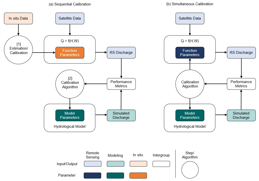
Figure 1 Two approaches to the calibration of macroscale hydrological models with discharge data retrieved from satellite data. (a) With sequential calibration, the discharge data are first estimated using a hydraulic model linking water level (H) and/or river width (W) to discharge (Q), and they are then used to calibrate the hydrological model. (b) With the second approach, both models are calibrated simultaneously.

Considering the increasing number of remotely sensed hydrological data that have become available over the last decades (Birkinshaw et al., 2010; Papa et al., 2012; Biancamaria et al., 2016) and that these satellite products are the only means to estimate river discharges in many regions of the world, the question arises as to how best use such remotely sensed data to support model calibration. Hence, the overarching questions that this paper addresses are as follows:

• To what extent is it possible and helpful to calibrate a macroscale hydrological model in ungauged catchments using remotely sensed data?

• How do we deal with potential interactions between parameters used in data preprocessing (i.e., from remotely sensed data to reconstructed discharge data) and parameters of the hydrological models when doing model calibration?

• Can we reduce the uncertainty from such interactions in model calibration results?

We answer these questions for an implementation of the VIC-Res hydrological model, a novel variant of the Variable Infiltration Capacity (VIC) model that includes a module for representing reservoir operations, for the Upper Mekong Basin (Dang et al., 2020a), an area characterized by the unavailability of discharge observations as well as major hydrological alterations caused by dam development (Hecht et al., 2019). To generate discharge time series for the calibration of VIC-Res, we use satellite altimetry data and a hydraulic model (based on Manning's equation) that is also identified from satellite data. In our framework, we first use global sensitivity analysis to demonstrate the existence of a pronounced codependence between the parameterization of the hydraulic model and the modeling accuracy of VIC-Res. To break this codependence, we leverage the results of the sensitivity analysis to constrain the parameterization of the hydraulic model and, thus, safely inform the calibration of VIC-Res, which is ultimately carried out using a multi-objective optimization approach.

2 Study site, model domain, and gauging stations

In this section, we provide information on our study site, the spatial domain of the hydrological model, and the availability of observed and remotely sensed discharge data.

2.1 The Lancang–Mekong Basin

Spanning an area of about 795 000 km², the Mekong River basin is the largest transboundary basin in Southeast Asia. The river is 4350 km long and stretches in a northwest–southeast direction from the Tibetan Plateau (approximately 5200 m a.s.l.) to the East Vietnam Sea (Fig. 2a). The basin can be roughly divided into two parts, namely, the Upper Mekong (also known as the Lancang in China) and the Lower Mekong, which is shared by five countries (Myanmar, Thailand, Laos, Cambodia, and Vietnam).

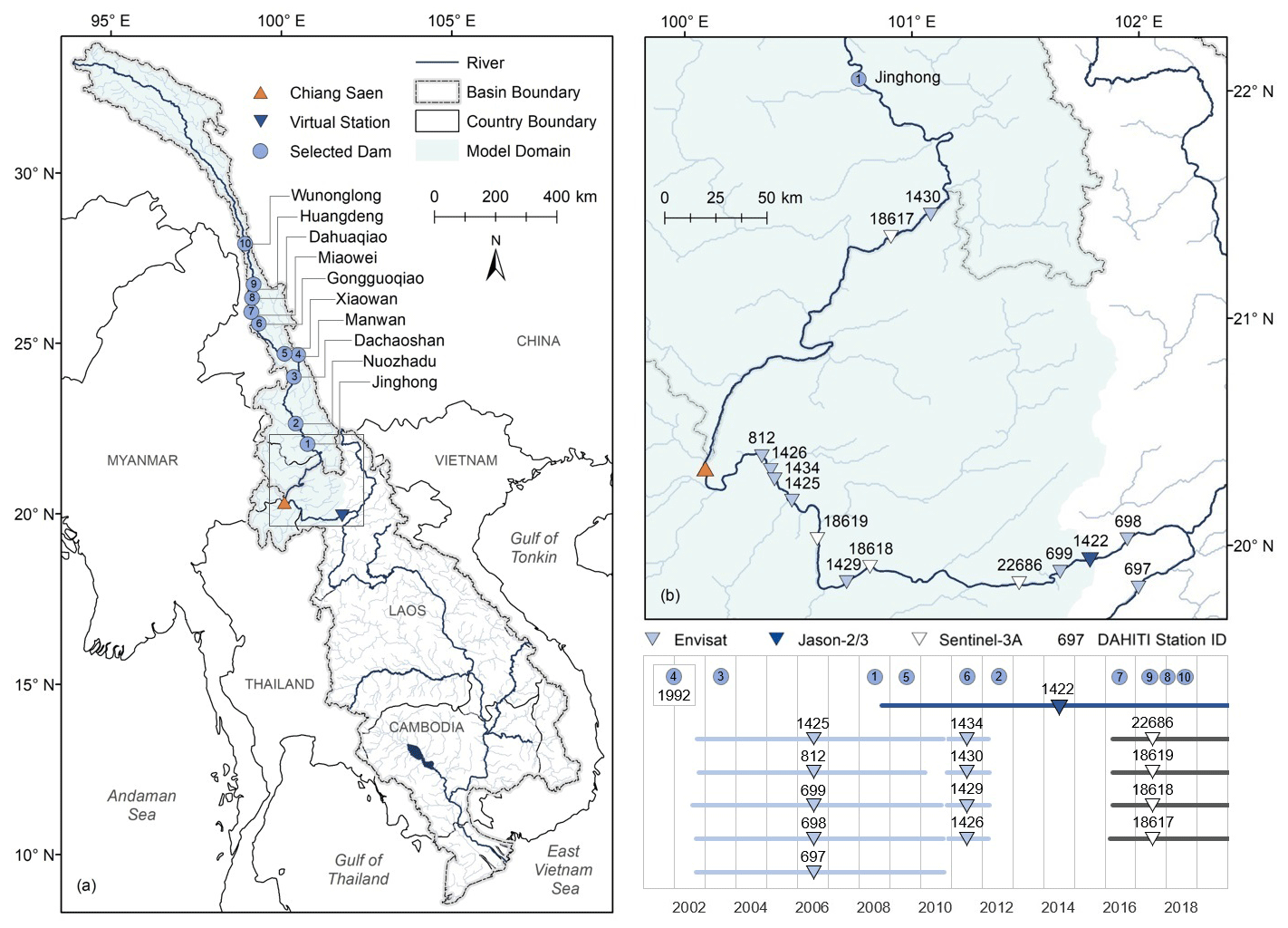
Figure 2 Panel (a) shows the Mekong River basin and its upper portion – the Lancang River basin. In this panel, we illustrate the location of the gauging station (Chiang Saen), the virtual gauging station, and 10 large hydropower dams on the main stem of the Lancang with a volume larger than 100×10⁶ m³ each, all included in the hydrological model. All dams are operational as of December 2020. The light green area is the spatial domain of the hydrological model. Panel (b) illustrates the locations around Chiang Saen where altimetry water level data are available. The data are collected by multiple satellites, namely, Envisat (light blue triangle), Jason-2/3 (dark blue triangle), and Sentinel-3A (white triangle), and are processed by the Database for Hydrological Time Series of Inland Waters (DAHITI). The number above each triangle corresponds to the station ID in DAHITI. The lower part of panel (b) illustrates the year that each dam was commissioned and the temporal coverage of altimetry data in each location, constrained by the operational period of the satellites. Location 1422 is chosen as our virtual station because of the temporal coverage and resolution of altimetry water level data at this location as well as its suitability with respect to the application of the methods for constructing a river cross-section and rating curve (see Sect. 3.2).

The Lancang accounts for 45 % of the river length, 21 % of the catchment area, and 16 % of the annual discharge of the entire Mekong (MRC, 2009). The complex topography of the Lancang Basin (high mountains and low valleys) contributes to the uneven spatial distribution of precipitation, which ranges from 600 mm yr⁻¹ on the Tibetan Plateau to 1700 mm yr⁻¹ in the mountains of Yunnan. Meanwhile, the monsoonal climate causes an uneven temporal distribution of precipitation, with 70 %–80 % of precipitation arriving in the wet season (June–November) (Yun et al., 2020).

Because of the advantageous topography and abundant water availability, the Lancang River basin has become a hotspot for hydropower development. Indeed, the Lancang dam system – developed over the past 3 decades – consists of more than 35 hydropower dams (WLE Mekong, 2022), including 10 large dams on the main stem with a volume larger than 100×10⁶ m³ each (see their location in Fig. 2a and specifications in Table S1 in the Supplement). The system has a total capacity of more than 42 000×10⁶ m³ and can control up to 55 % of the annual flow to northern Thailand and Laos. The Lancang River basin is an excellent example of a transboundary and heavily regulated river with limited information on dam operations: initiatives on the sharing of year-round water data are still in their infancy (Johnson, 2020), so the only data available to the public are those retrieved from satellite data (e.g., Bonnema and Hossain, 2017; Biswas et al., 2021; Vu et al., 2022). Time series of river discharge measured within China's political boundaries are not available.

2.2 Model domain and study period

The spatial domain of our hydrological model is the light green area illustrated in Fig. 2. This domain corresponds to the Lancang Basin (namely, the area falling within China's political boundaries) as well as an additional area spanning across Myanmar, Thailand, and Laos. Note that the domain of hydrological models focusing on the Lancang is typically “closed” at Chiang Saen (e.g., Dang et al., 2020a), where the first gauging station with publicly available data is located. Here, we slightly extend the domain so as to account for the location of a virtual gauging station (see Sect. 2.3). The simulation period is from 2009 to 2018 and, thus, comprises the main development of the Lancang reservoir system, including the filling period of the two largest reservoirs, Xiaowan and Nuozhadu, which account for ∼85 % of the total system's storage (Vu et al., 2022). Another reason for the choice of this study period is to make it compatible with the temporal coverage of altimetry data at our virtual station, which we describe next.

2.3 Gauging stations

As mentioned above, the first gauging station with publicly available data is Chiang Saen, located in northern Thailand, about 350 km from Jinghong Dam (Fig. 2). Daily water level and discharge at the station have been collected since 1990 by the Mekong River Commission (MCR) and are available on its online data portal (https://portal.mrcmekong.org/, last access: 22 December 2022). As we developed a methodology for calibrating models in ungauged river basins, these data are used only for model validation.

To infer the discharge time series needed for model calibration, we sought locations around Chiang Saen where altimetry water level data are available (Fig. 2b). From these data, one can try to infer the river discharge. These data are collected by multiple satellites (i.e., Envisat, Jason-2/3, and Sentinel-3A) and are available in the Database for Hydrological Time Series of Inland Waters (DAHITI, https://dahiti.dgfi.tum.de/, last access: 22 December 2022). In this study, we choose location 1422 (Jason-2/3) – about 280 km downstream of Chiang Saen – as our virtual gauging station (virtual station hereafter). This is because of two main reasons. First, the temporal coverage of data at the chosen location covers the years in which the majority of the dams were commissioned, including the two largest reservoirs, Xiaowan and Nuozhadu (see the lower part of Fig. 2b). Second, the temporal resolution of Jason-2/3 (10 d) is finer than that of Envisat (35 d) and Sentinel-3A (27 d). It is also worth noting that another database, Hydroweb (https://hydroweb.theia-land.fr/, last access: 22 December 2022), provides (Sentinel-3A/B) altimetry water level data for a number of locations at our study site. However, these data have the same temporal resolution and coverage as the Sentinel-3A data provided by DAHITI, which makes them unsuitable for our study. Moreover, the methods used to construct a river cross-section and rating curve at the virtual station work best for location 1422 (see Sect. 3.2).

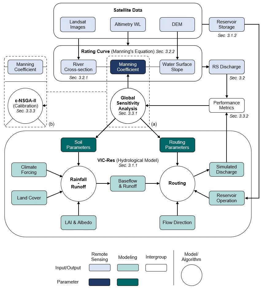
Figure 3 Flowchart illustrating our numerical framework. The VIC-Res model (green boxes) includes a rainfall–runoff and a routing module; the latter explicitly simulates reservoir operations using data retrieved from satellite observations. The discharge data used to calibrate VIC-Res are estimated from altimetry water levels through a rating curve, which is based on Manning's equation and developed using multiple satellite data (Landsat images, altimetry water level, and a digital elevation model). All remote sensing items are represented by blue boxes. The relationship between the parameterization of Manning's equation (dark blue box) and the performance of VIC-Res is assessed and quantified via global sensitivity analysis (a). Based on the results of the sensitivity analysis, we then set a value of Manning's coefficient and calibrate the parameters of VIC-Res using a non-dominated sorting genetic algorithm (ε-NSGA-II) for multi-objective optimization (b).

3 Methodology

The numerical framework developed for our study consists of two main modeling components (illustrated in Fig. 3). We model the hydrological processes within the Lancang Basin with VIC-Res, whose routing module includes an explicit representation of reservoir operations (Sect. 3.1). The discharge data at the virtual station used to calibrate VIC-Res are generated by a simple hydraulic model, namely, a rating curve based on Manning's equation (Sect. 3.2). In our approach, we first use global sensitivity analysis to explore the relationship between the parameterization of the rating curve and the performance (fit to data) that can be achieved through calibration of VIC-Res (Sect. 3.3). Then, we use the knowledge gained through this sensitivity analysis to select the parameterization of the rating curve and proceed with the calibration and validation of VIC-Res.

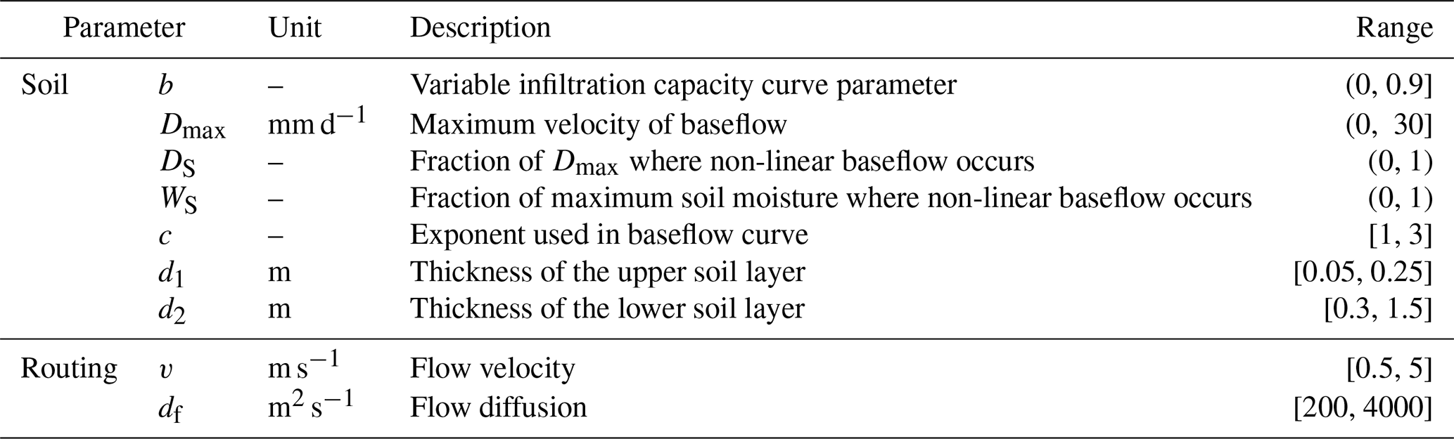
Table 1 Soil parameters controlling the rainfall–runoff process and routing parameters in VIC-Res. The last column shows the range of each parameter considered in this study and also adopted in previous studies (e.g., Dan et al., 2012; Park and Markus, 2014; Xue et al., 2015; Wi et al., 2017).

3.1 Modeling hydrological processes and reservoir operations

3.1.1 Hydrological model

The hydrological model used in this study is VIC-Res (Dang et al., 2020a), a novel variant of VIC, which is a macroscale, semi-distributed hydrological model developed by the University of Washington (Liang et al., 2014). Both VIC and VIC-Res consist of two modules, namely, a rainfall–runoff and a routing module (Fig. 3). In the rainfall–runoff module, the study region is divided into computational cells with a customizable cell size (0.0625^∘ in this study). For each cell, the key hydrological processes (evapotranspiration, infiltration, baseflow, and runoff) are calculated as a function of various inputs, including climate forcing (e.g., precipitation, temperature, and wind speed), land cover, leaf area index, and albedo. In the routing module, simulated baseflow and runoff produced by the first module are routed throughout the river network, with the routing process modeled by the linearized Saint-Venant equation (Lohmann et al., 1996, 1998).

Improving on the VIC model, VIC-Res includes an explicit representation of water reservoir operations. For each reservoir in the study region, the model solves the storage mass balance and calculates the reservoir release. Specifically, we leverage information on modeled inflow and estimated storage (see Sect. 3.1.2). These two variables are combined with information on evaporation (simulated using the estimated water surface area and evaporation rates calculated with the Penman equation) to invert the mass balance equation, yielding the reservoir release. Additional details on VIC-Res, including alternative approaches to reservoir operations, are described in Dang et al. (2020b).

In our VIC-Res model, we calibrate seven soil parameters and two routing parameters (see Table 1). The soil parameters controlling the rainfall–runoff process are b, D_max, D_S, W_S, c, d₁, and d₂. To be more specific, the parameter b is the VIC curve parameter, which determines the infiltration capacity and surface runoff amount generated by each cell (Ren-Jun, 1992; Todini, 1996). In particular, higher values of b produce less infiltration and more surface runoff. D_max, D_S, W_S, and c are the baseflow parameters, which influence the shape of the baseflow curve (Franchini and Pacciani, 1991). Specifically, D_max is the maximum velocity of baseflow, D_S is the fraction of D_max at which non-linear baseflow begins, and W_S is the fraction of maximum soil moisture at which non-linear baseflow begins. The parameter c is the exponent used in the baseflow curve. d₁ and d₂ are the thickness of the two soil layers. Thicker layers increase the water storage capacity and, hence, increase the evaporation losses. Thicker soil layers also delay the seasonal peak flow. The routing parameters are flow velocity (v) and flow diffusion (d_f).

The data used in our VIC-Res model consist of climate forcing data, land use and cover, leaf area index (LAI), albedo, flow direction, and time series of reservoir storage volume. Climate forcing data include daily precipitation data retrieved from the CHIRPS-2.0 dataset, daily maximum and minimum temperature, and wind speed (retrieved from the ERA5 dataset). We collect land use and cover data from the Global Land Cover Characterization (GLCC) dataset and soil data from the Harmonized World Soil Database (HWSD). Monthly LAI and albedo are derived from the Terra MODIS satellite images, while the flow direction is calculated from the Shuttle Radar Topography Mission (SRTM)  digital elevation model (DEM) data. The monthly time series of reservoir storage volume are reconstructed from satellite data, as explained below.

We finally note that the choice of the cell size could affect the rainfall–runoff and routing estimations, thereby impacting model calibration and simulated discharge (Egüen et al., 2012). As the issue applies to any modeling exercise, not only to those relying on remotely sensed data like this study, we do not carry out an analysis of the impact of cell size on model performance. Instead, we choose a cell size (i.e., 0.0625^∘) that falls in between what is currently being adopted for the existing distributed models for the Mekong region. For example, Costa-Cabral et al. (2007) and Tatsumi and Yamashiki (2015) adopted a resolution of $\mathrm{1}/\mathrm{12}$ and 0.25^∘, respectively, while Du et al. (2020) and Bonnema and Hossain (2017) used a resolution of $\mathrm{90}/\mathrm{900}$ m and 0.01^∘, respectively.

3.1.2 Reservoir operations

To capture the actual operations of reservoirs, we use monthly time series of reservoir storage volume reconstructed from satellite data by Vu et al. (2022). Specifically, the time series of reservoir storage volume are obtained from Landsat images (Landsat 5 available from 1984 to 2013, Landsat 7 from 1999 to 2022, and Landsat 8 from 2013 to present) and a digital elevation model (SRTM DEM). The time series are created via three steps. First, the relationship between water surface area and storage volume (the area–storage curve) for each reservoir is calculated from DEM data. Then, the reservoir water surface area is estimated from Landsat images by a water surface area estimation algorithm that removes the effects of clouds and other disturbances (Gao et al., 2012; Zhang et al., 2014). Finally, the storage volume is inferred from the water surface area through the area–storage curve. The results obtained from Landsat images are validated with altimetry water levels (Jason-2 available from 2008 to 2016, Jason-3 from 2016 to present, and Sentinel-3 from 2016 to present) for the reservoirs where altimetry water levels are available. As the VIC-Res model adopts a daily simulation time step, the monthly time series of reservoir storage volume is interpolated to daily values. Although using interpolated values (monthly to daily) is not ideal, it is reasonable to do so if one considers the specific characteristics of the reservoir system. In particular, Xiaowan and Nuozhadu are the two largest reservoirs: they have a massive capacity (∼36 km³) and account for about 85 % of the total system’s storage. Because of their size, their role is not to follow inter- and intra-daily electricity demand variability but rather to ensure a stable supply of power and to minimize the variability in the production of the other dams composing the hydropower system. This goal is reflected by their operating patterns. In the wet season (June–November), the Xiaowan and Nuozhadu reservoirs gradually store water until they reach their maximum operational level (and release extra water if necessary). The other reservoirs run at their normal operational level (full capacity for power generation). In the dry season (December–May), Xiaowan and Nuozhadu gradually release water to the downstream reservoirs to ensure that the other reservoirs can run at their normal operational level (International Rivers, 2014). Therefore, it is fair to state that Xiaowan and Nuozhadu are characterized by slowly varying dynamics. Additionally, the analysis carried out in Vu et al. (2022) shows a strong similarity between the monthly storage of Xiaowan and Nuozhadu derived from Landsat images and the storage derived from Jason altimetry data (10 d temporal resolution) and Sentinel-1/2 images (6 d temporal resolution). Because of the spatial and temporal coverage of those data, we use the result derived from Landsat images for this study.

3.2 Inferring discharge data

To handle the lack of discharge data for model calibration, we again resort to satellite data. Specifically, we convert altimetry water levels (Jason-2/3) to discharge through a rating curve specified for the location of the virtual station (see Fig. 3). The rating curve (i.e., Manning's equation) is identified based on the information on the river cross-section and water surface slope at the virtual station, which is also derived from satellite data.

3.2.1 River cross-section

We construct the river cross-section at the virtual station using multiple satellite products (see Fig. S1a in the Supplement). First, we use a digital elevation model (SRTM DEM), which has a spatial resolution of 30 m, to obtain the portion of the cross-section above the water level at the observation time of the SRTM satellite (February 2000). To extend the information available to estimate the river cross-section, we then pair data on river widths at the virtual station with the corresponding water levels (nearest observations in time from the two satellites that provide river widths and water levels) (Bose et al., 2021). River widths are estimated from the water pixels – classified from Landsat images based on the normalized difference water index (NDWI) – along the river cross-section. The NDWI is calculated using the green and near-infrared bands of Landsat images: NDWI = (green band − near-infrared band)$/$(green band + near-infrared band) (Zhai et al., 2015). All of these bands have a spatial resolution of 30 m. Meanwhile, the water level data are processed from Jason-2/3 altimetry satellite data provided by DAHITI. Finally, for each riverbank, we use a regression model (sixth-degree polynomial), which is the best fit to the data points obtained from the two first steps. The two models help us extrapolate the portion of the river cross-section under the lowest water level observed by the satellites. It is worth noting that the approach works best for river banks under natural conditions, where it is possible to infer the relation between river widths and water levels. It would be challenging to apply this approach at Chiang Saen, for example, where the river banks have been engineered.

3.2.2 Rating curve

We construct the rating curve at the virtual station with Manning's equation (Eq. 1):

$$\begin{array}{}\text{(1)}& Q={\displaystyle \frac{A^{\mathrm{5}/\mathrm{3}}{S}^{\mathrm{1}/\mathrm{2}}}{P^{\mathrm{2}/\mathrm{3}}n}},\end{array}$$

where Q, A, and P are the respective discharge, river cross-section area, and wet perimeter corresponding to the water depth D (see Fig. S1b). As explained next, A and P are calculated from the river cross-section for different values of water depth D. S is the hydraulic slope, estimated from DEM data (which reflect the water surface slope at the observation time). n is the Manning coefficient (riverbed roughness); following Chow (1959) and Engineering ToolBox (2004), we assume that it ranges from 0.03 to 0.06.

The rating curve is constructed in two steps. First, we use Eq. (1) to estimate the discharge corresponding to each water depth with regular intervals of 1 m (e.g., 0, 1, and 2 m). After this step, we have a number of data points at hand, each containing a value of the water depth and its corresponding discharge. Then, we fit the data points using a power curve. This translates into our rating curve. Note that, when converting altimetry water level to discharge using the rating curve, we convert altimetry water level to water depth by deducting the riverbed elevation (Fig. S1b). It is worth noting that this approach, based on Manning's equation, works best for straight river segments with limited discharge variations due to tributaries and distributaries nearby (Przedwojski et al., 1995). This condition and the condition for constructing the river cross-section mentioned above make location 1422 the most suitable location for our virtual station, despite the fact that there are other locations closer to Chiang Saen (e.g., the location 812) that could provide a better validation using observed data at Chiang Saen.

3.3 Sensitivity analysis and model calibration

3.3.1 Sensitivity analysis

We carry out a global sensitivity analysis (Pianosi et al., 2016) to study the relationship between the performance of VIC-Res and the parameterization of the rating curve. We investigate a total of 10 model parameters, including 7 soil parameters of the rainfall–runoff module, 2 parameters of the routing module, and the Manning coefficient appearing in the rating curve. We use Latin hypercube sampling to create 1000 samples in the 10-dimensional parameter space defined by the ranges given in Sect. 3.1.1 and 3.2.2. For each parameter sample, we run a simulation over the period from 2009 to 2018 (after a warm-up period from 2005 to 2008) and then reconstruct discharge data for the same period with the rating curve. We then compare reconstructed and simulated discharges through four performance metrics, which are described in the next subsection. Having built this input (parameters) and output (performance metrics) dataset, we analyze the codependence between the performance of VIC-Res and the Manning coefficient. We also identify the parameter samples that map into the top 25 % of samples yielding the best performance with respect to each metric and analyze if (and how) such performance constraints map back into parameter value constraints. The simulation experiment is run on a 2.50 GHz Intel^® Xeon^® W-2175 CPU with 128 GB RAM running Linux Ubuntu 18.04. The total running time is about 200 h.

3.3.2 Performance metrics

The performance metrics are calculated by comparing the simulated (by VIC-Res) and remotely sensed discharge at the virtual station. Because the temporal resolution of remotely sensed discharge is defined by the revisit time of the altimetry satellite (approximately 10 d for Jason-2/3), we calculate the performance metrics using the data of all days on which altimetry water levels are available. Among the several metrics available in literature (Dawson et al., 2010), we chose four metrics that explicitly capture different aspects of modeling accuracy: the Nash–Sutcliffe efficiency (NSE), the transformed root-mean-square error (TRMSE), the mean-squared derivative error (MSDE), and the runoff coefficient error (ROCE). The NSE and TRMSE assess the model performance on high and low flows, respectively, while the MSDE accounts for the shape of the hydrograph timing errors and for noisy signals. Finally, the ROCE assesses the overall water balance (Reed et al., 2013). The metrics are defined as outlined in the following.

$$\begin{array}{}\text{(2)}& \mathrm{NSE}=\mathrm{1}-{\displaystyle \frac{\sum _{t=\mathrm{1}}^n{\left(Q_{\mathrm{Sim},t}-Q_{\mathrm{RS},t}\right)}^{\mathrm{2}}}{\sum _{t=\mathrm{1}}^n{\left(Q_{\mathrm{RS},t}-\stackrel{\mathrm{‾}}{Q_{\mathrm{RS}}}\right)}^{\mathrm{2}}}},\end{array}$$

where n is the number of satellite altimetry water level observations, Q_Sim,t and Q_RS,t are the respective simulated and remotely sensed discharge at the virtual station (for the observation number t), and $\stackrel{\mathrm{‾}}{Q_{\mathrm{RS}}}$ is the mean of the remotely sensed discharge.

$$\begin{array}{}\text{(3)}& \mathrm{TRMSE}=\sqrt{{\displaystyle \frac{\mathrm{1}}{n}}\sum _{t=\mathrm{1}}^n{\left(z_{\mathrm{Sim},t}-z_{\mathrm{RS},t}\right)}^{\mathrm{2}}},\end{array}$$

where z_sim,t and z_RS,t represent the respective values of the simulated and remotely sensed discharge at the virtual station (for the observation number t), both transformed by the expression $z=\frac{(\mathrm{1}+Q{)}^{\mathit{\lambda }}-\mathrm{1}}{\mathit{\lambda }}$ (λ=0.3). In other words, λ scales down the values of the discharge, thereby emphasizing the errors on low flows.

$$\begin{array}{}\text{(4)}& {\displaystyle }& {\displaystyle }\mathrm{MSDE}={\displaystyle \frac{\sum _{t-\mathrm{1}}^n{\left(\left(Q_{\mathrm{RS},t}-Q_{\mathrm{RS},t-\mathrm{1}}\right)-\left(Q_{\mathrm{Sim},t}-Q_{\mathrm{Sim},t-\mathrm{1}}\right)\right)}^{\mathrm{2}}}{n-\mathrm{1}}}\text{(5)}& {\displaystyle }& {\displaystyle }\mathrm{ROCE}=abs\left({\displaystyle \frac{\stackrel{\mathrm{‾}}{Q_{\mathrm{Sim}}}}{\stackrel{\mathrm{‾}}{P}}}-{\displaystyle \frac{\stackrel{\mathrm{‾}}{Q_{\mathrm{RS}}}}{\stackrel{\mathrm{‾}}{P}}}\right)\end{array}$$

Here, $\stackrel{\mathrm{‾}}{Q_{\mathrm{Sim}}}$ is the mean of the simulated discharge at the virtual station and $\stackrel{\mathrm{‾}}{P}$ is the mean annual rainfall.

3.3.3 Model calibration

As we shall see, the global sensitivity analysis helps us understand the relationship between the performance of VIC-Res and the parameterization of the rating curve. Moreover, by identifying the parameter samples that map into high values of the performance metrics (here the top 25 %), the analysis helps us narrow down the range of variability in (at least some of) the model parameters. However, one may still want to complete the model calibration by further seeking for combinations of the VIC-Res parameters that optimize the performance metrics. To this end, we couple VIC-Res with ε-NSGA-II, a multi-objective evolutionary algorithm widely used for hydrological modeling applications (Reed et al., 2013; Dang et al., 2020a). Here, the decision variables are the nine parameters of VIC-Res, while the objective function is a vector consisting of the four metrics described in Sect. 3.3.2. Similarly to the sensitivity analysis, all metrics are calculated via simulation over the period from 2009 to 2018, with a spin-up period going from 2005 to 2008. The ε-NSGA-II is set up with ε=0.001, an initial population size of 10, and a number of function evaluations equal to 100. All performance metrics are normalized between zero and one. The calibration exercise is carried out on 10 independent trials, with the best (Pareto-efficient) parameter combinations selected across the 10 calibration exercises. The total runtime is about 210 h (using the same computational infrastructure adopted for the sensitivity analysis).

4 Results

Here, we move across three steps. First, we illustrate the results leading to the estimation of a discharge time series at the virtual station, including the identification of the river cross-section and rating curve (Sect. 4.1). Then, we use sensitivity analysis to show that a codependence exists between the Manning coefficient and the performance of VIC-Res, and we propose an approach to overcome this potential issue (Sect. 4.2). We finally calibrate VIC-Res and validate its performance using observed discharge data at Chiang Saen (Sect. 4.3).

4.1 Estimation of the remotely sensed discharge at the virtual station

4.1.1 River cross-section

Figure 4a shows the river cross-section at the virtual station, constructed via the use of multiple satellite data. Specifically, each dark blue bar represents a 30 m cell of the SRTM DEM lying along the river cross-section. These bars are connected by a series of segments representing an estimate of the cross-section above the water surface at the observation time of the SRTM satellite. That specific water surface is depicted by the horizontal dark blue line at an elevation of 293 m. The light blue lines indicate the river widths derived from 19 Landsat 5 images and water levels obtained from Jason-2/3. Additional information about these images, water levels, and corresponding collection dates are reported in Table S2 in the Supplement. Finally, the dotted blue line represents the cross-section below the lowest observed water level. This line is created via extrapolation by two regression models (sixth-degree polynomial), which are fitted to the observations retrieved from the DEM, Landsat 5, and Jason-2/3 (11 and 14 data points for the left and right banks, respectively). We also explore four alternative cross-sections, created by moving the one at the location of the virtual station 30 and 60 m (one and two cells) both upstream and downstream, with the assumption that water levels at the alternative cross-sections are the same as those at the virtual station (water surface slope around the virtual station estimated from the DEM is about 0.00015≈8.8 mm/60 m). The alternative cross-sections are in good agreement with the cross-section at virtual station (see Fig. S2). Specifically, riverbed elevations are 277.2, 275.6, 276, 274.5, and 274.3 m a.s.l. (from upstream to downstream).

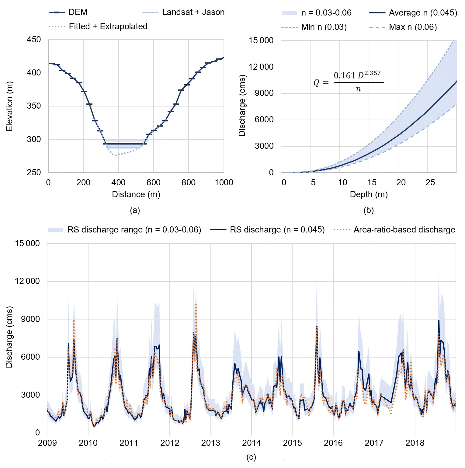
Figure 4 (a) River cross-section at the virtual station constructed from multiple satellite data. The dark blue line is obtained from a SRTM DEM, while the light blue lines are retrieved by pairing Landsat-derived river widths with Jason altimetry water levels. The dotted blue line is created using two regression models, which are first fitted to the right and left banks and then extrapolated to the portion below the lowest observed water level. Panel (b) shows the range of variability in the rating curve (at the virtual station) for values of n ranging from 0.003 to 0.006 (light blue band). In this plot, we also illustrate three rating curves corresponding to specific values of n: minimum (dotted blue line), average (dark blue line), and maximum (dashed blue line). Panel (c) presents remotely sensed (RS) discharge at the virtual station. The light blue band represents the range of variability, with n varying from 0.03 to 0.06. The dark blue line is the estimated discharge with the average value of n (0.045). Note that this time series is relatively similar to the one obtained by scaling the discharge measured at Chiang Saen by the area ratio (equal to 1.17). That time series is depicted by the dotted orange line. The unit “cms” on the y axes represents cubic meters per second.

4.1.2 Rating curve

With the river cross-section at hand, we estimate the rating curve at the virtual station using Manning's equation (Eq. 1). As the value of the Manning coefficient n is unknown, the value of the estimated discharge Q depends not only on the water depth D but also on n, that is

$$\begin{array}{}\text{(6)}& Q={\displaystyle \frac{\mathrm{0.161}{D}^{\mathrm{2.357}}}{n}}.\end{array}$$

In Fig. 4b, we plot the range of variability in the rating curve corresponding to values of n varying between 0.03 and 0.06 (Sect. 3.2.2). This range is represented by the light blue band. Note the large increase in river discharge estimates corresponding to a depth larger than 20 m. In this figure, we also report three rating curves corresponding to three specific values of n, namely, the minimum (dotted blue line), average (dark blue line), and maximum (dashed blue line).

4.1.3 Remotely sensed discharge

Using the rating curve and water depth (converted from Jason-2/3 altimetry water level data), we estimate 298 discharge data points at the virtual station during the period from 2009 to 2018 (Fig. 4c). The light blue band represents the envelope of variability in the discharge corresponding to values of n ranging between 0.03 and 0.06. The figure also depicts the discharge time series corresponding to the average value of the Manning coefficient (n=0.045) as well as an additional time series obtained by scaling the observed discharge at Chiang Saen by a coefficient (equal to 1.17) representing the relative increase in drainage area between Chiang Saen and the virtual station (dotted orange line). A qualitative comparison of these estimated discharge values provides a few useful insights. First, there is large uncertainty in the discharge estimated during the summer monsoon season. This result is explained by the characteristics of the rating curve – the higher the value of D, the higher the uncertainty in Q (Fig. 4b). Second, there is a larger variability in the discharge estimated during the dry season of 2013–2018 compared with that of 2009-2012. That is because the cascade dam system in the Lancang modified the natural flow downstream, increasing low flows (Vu et al., 2022). The change can be seen most clearly since 2013, when Nuozhadu, the largest reservoir in the system, became operational. Moreover, it should be considered that the discharge variability could be further amplified by the use of a rating curve; recall that when converting water level to discharge, the higher the water depth value, the larger the discharge variability (Fig. 4b). Lastly, there seems to be a reasonable agreement between the discharge time series corresponding to n=0.045 and that estimated from values observed at Chiang Saen. This implicitly validates the rating curve, further suggesting that the mean value of n might be a reasonable estimate. To further investigate this last point – and understand how the choice of the Manning coefficient influences the performance of VIC-Res – we now move to the sensitivity analysis.

4.2 Sensitivity analysis

4.2.1 Codependence between VIC-Res performance and the Manning coefficient

The first fundamental step in our analysis is to understand whether co-estimating the Manning coefficient and the parameters of the hydrological model (see Fig. 1) could bias the calibration process, ultimately limiting the reliability of VIC-Res. To answer this question, we leverage the results obtained by exploring (via simulation) 1000 different parameterizations of VIC-Res and Manning's equation.

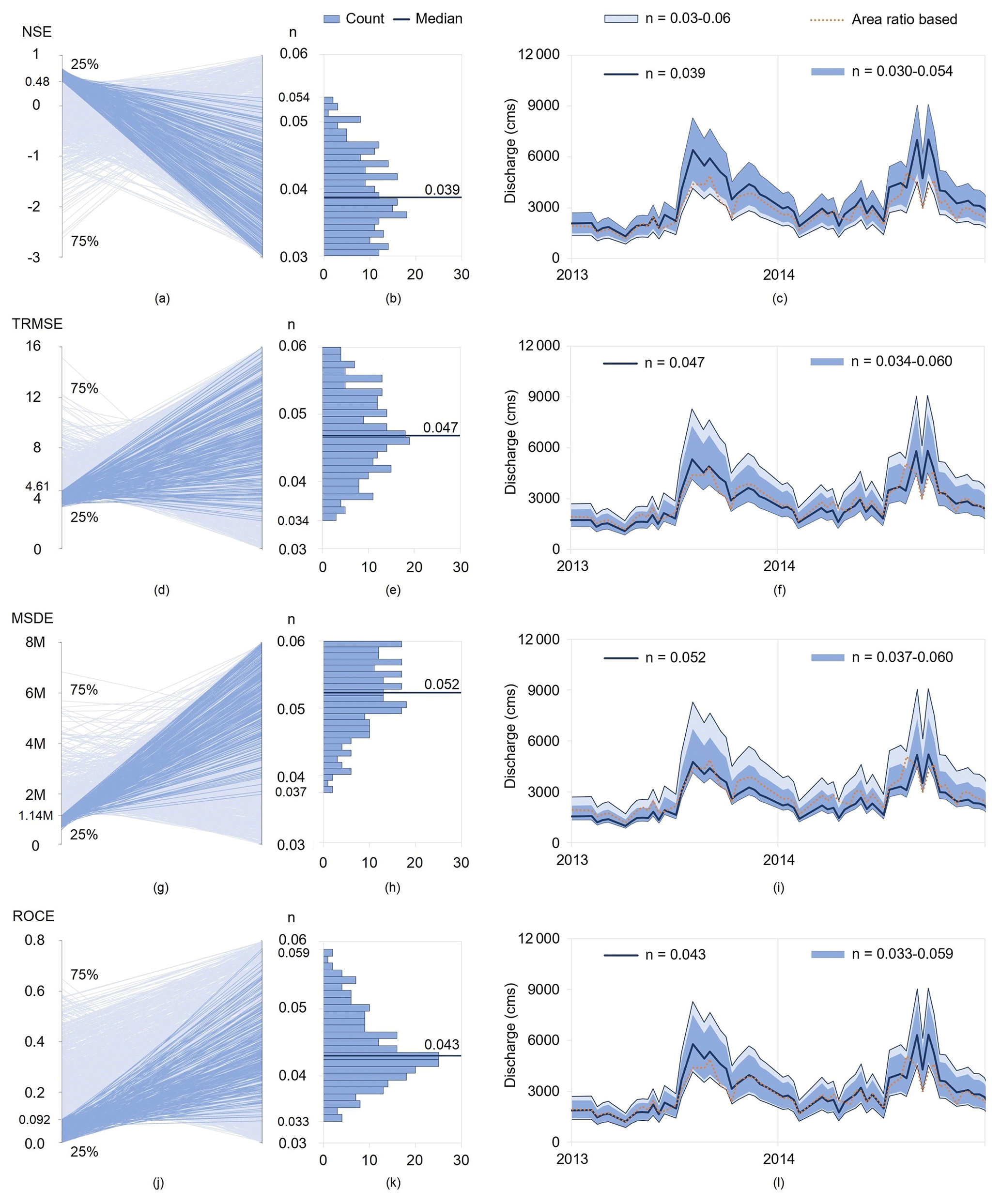
Figure 5 The first column contains four parallel-coordinate plots. In each plot, the left axis is a model performance metric (i.e., NSE, TRMSE, MSDE, or ROCE) and the right axis is the Manning coefficient n. Each line corresponds to one of the 1000 parameterizations generated by Latin hypercube sampling. The dark blue lines highlight the top 25 % of parameterizations yielding the best performance for each metric. The histograms in the second column illustrate the frequency distribution of n corresponding to these top 25 % of parameterizations. The median is depicted by the dark blue line. In the last column, we report (in light blue) the range of variability in the discharge estimated with $n\in [\mathrm{0.03},\mathrm{0.06}]$ (this is the same range as in Fig. 4c) and (in dark blue) the range corresponding to the top 25 % of parameterizations with the best performance for each metric. The black lines present the discharge corresponding to the four median values of n (see the second column) and the dotted orange line is the discharge estimated from observations at Chiang Saen via the area-ratio-based method. Note how the use of different performance metrics results in different ranges and different medians of the Manning coefficient. The unit “cms” on the y axes represents cubic meters per second.

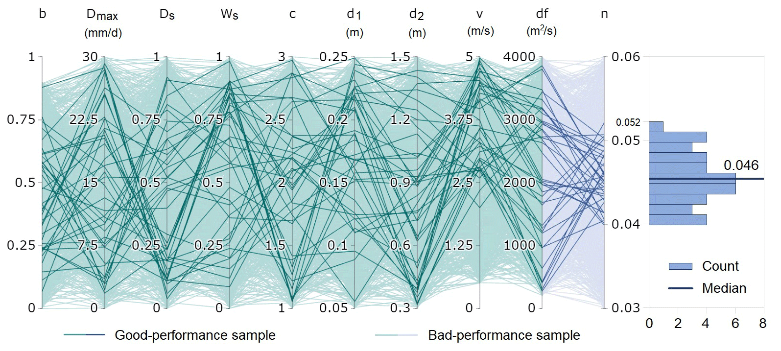
Figure 6 Parallel-coordinate plot illustrating the 1000 parameterizations explored in this study. The first nine axes (green) represent the VIC-Res model parameters, while the last axis (blue) represents the Manning coefficient n. Darker lines highlight the 40 parameterizations showing good performance for all metrics; these are identified by intersecting the four groups of parameterizations (each group is the top 25 % of parameterizations yielding the best performance for each metric). The panel on the right illustrates the frequency distribution of n corresponding to the 40 selected parameterizations. The median of this distribution is 0.046.

In Fig. 5a, d, g, and j, we illustrate the relationship between the four metrics of performance calculated for VIC-Res (i.e., NSE, TRMSE, MSDE, and ROCE) and the value of the Manning coefficient n. To aid the analysis, we highlight (in a darker color) the parameterizations yielding the top 25 % of samples yielding the best performance (250 samples) with respect to each metric. For example, in Fig. 5a, the 250 samples with a higher NSE are represented by the dark blue lines, whereas the 750 samples with a lower NSE are represented by the light blue lines. The NSE threshold created by the top 25 % is equal to 0.48. Interestingly, when comparing these four panels, we see that the values of n corresponding to the best performance vary with the metric that we consider. For example, the performance of the top 25 % of parameterizations yielding the highest values of NSE is given by values of n ranging between 0.03 and 0.054, whereas those giving the best performance for the MSDE range between 0.037 and 0.06. This point is consolidated by Fig. 5b, e, h, and k, where we show the frequency distribution of n corresponding to the performance of the top 25 % of samples for each metric. The minimum and maximum values that we found for each distribution are [0.03, 0.054], [0.034, 0.06], [0.037, 0.06], and [0.033, 0.059] for the NSE, TRMSE, MSDE, and ROCE, respectively. Note also how the median value of each distribution changes with the selected performance metric.

The explanation behind this result must be sought in the different aspects of the simulated hydrograph that are captured by the four metrics (see Sect. 3.3.2). Let us consider, for instance, the NSE, a metric that emphasizes model performance on high flows: the top 25 % of parameterizations of VIC-Res achieving the best performance are those corresponding to smaller values of n, which translate (via Manning's equation) into higher discharge estimates. In other words, calibrating both models simultaneously while using the NSE as a performance metric leads to producing discharge data that are biased towards higher values (Fig. 5c). Similarly, the values of n associated with the best TRMSE and MSDE performance are shifted upward (i.e., producing lower discharges), as both metrics emphasize model accuracy on lower flows (Fig. 5f, i). For the ROCE, most values of n are concentrated around the median value of 0.043 (close to the mean of 0.045). Note that ROCE the looks at the overall water balance, thereby requiring calibration of the hydrological models on discharge values that are more centered towards the bulk of the distribution (Fig. 5l).

4.2.2 Breaking the codependence

Having established that there can be a codependence between the performance of VIC-Res and the Manning coefficient, we now turn our attention to a potential solution. Ideally, one would like to calibrate a hydrological model that performs well with respect to multiple performance metrics (Efstratiadis and Koutsoyiannis, 2010). Guided by this simple concept, we consider the parameterizations of VIC-Res and Manning's equation associated with the top 25 % of parameterizations with the best performance with respect to all metrics (i.e., NSE, TRMSE, MSDE, and ROCE). This leaves us with 40 parameterizations (illustrated in Fig. 6). The first interesting point to note in the figure (right panel) is the empirical distribution of n. Focusing on satisfactory performance across multiple metrics yields a narrower range of the Manning coefficient concentrated around the median value of 0.046. As we shall see later, this means that the uncertainty in discharge values is reduced with respect to what we observed in Fig. 5.

The left panel of Fig. 6 illustrates the specific values of the parameterizations through a parallel-coordinate plot, in which each axis represents a parameter and each line is a parameter sample. The 40 top-performing parameterizations are highlighted in bold, whereas the remaining 960 are depicted with a lighter color. Here, we notice that only the range of the flow velocity (v) can be clearly narrowed down (in addition to n, of course). Specifically, when considering only the 40 top-performing parameterizations, the range is reduced from [0.5, 5] to [2, 5]. For some parameters (i.e., b, d₁, and d₂), although their ranges remain fairly large, the values in the 40 top-performing combinations are mostly (but not exclusively) concentrated in certain parts of the initial range: for b, in the middle part (0.2 to 0.75); for d₁ in the upper part (0.12 to 0.25); for d₂ in the lower part (0.3 to 1). Lastly, for the remaining parameters (i.e., D_max, D_S, W_S, c, and d_f), the 40 top-performing samples are evenly distributed throughout the initial range. This is a common problem in macroscale hydrological models, including VIC (Yeste et al., 2020), a point to which we will return in Sect. 5.

4.2.3 Narrowing the uncertainty in discharge data

How does the new parameterization of n impact the remotely sensed discharge data needed to calibrate the model? To answer this question, we compare two envelops of variability for the discharge data in Fig. 7a: the one (light blue envelope) corresponding to $n\in [\mathrm{0.03},\mathrm{0.06}]$ (the initial uncertainty range of n) and the one (dark blue envelope) corresponding to $n\in [\mathrm{0.04},\mathrm{0.052}]$ (the narrowed range after constraining across all four metrics; see Sect. 4.2.2). As expected, the range of remotely sensed discharge is narrowed down significantly, especially during the high-flow periods. Another point that is worth noticing here is that the discharge time series corresponding to the median value of n (i.e., 0.046) is close to the time series estimated from the data available at Chiang Saen. This is a qualitative, yet informative, validation of the sensitivity analysis results.

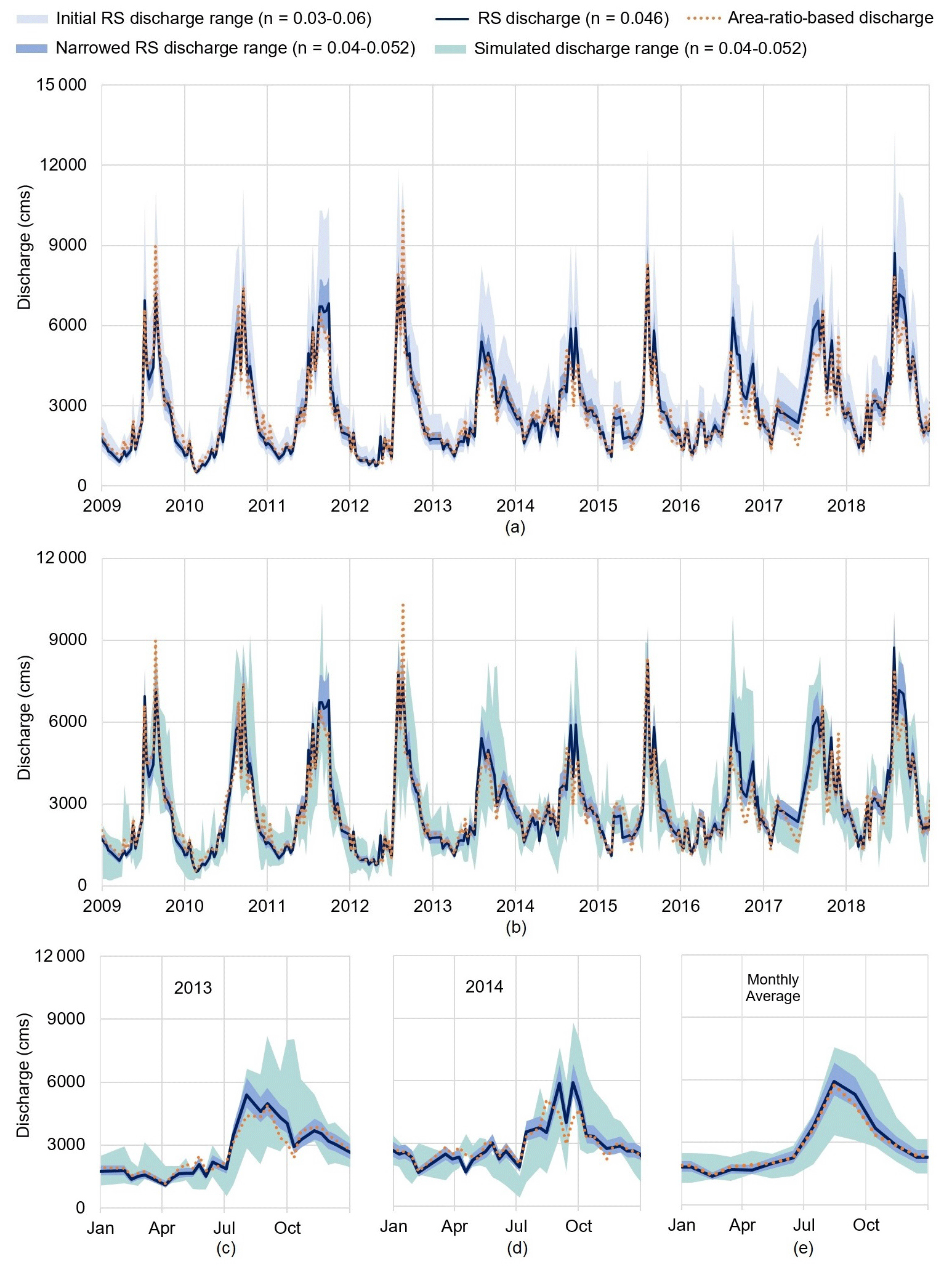
Figure 7 In panel (a), we compare the range of variability in the remotely sensed (RS) discharge before and after sensitivity analysis. The two envelopes correspond to values of n belonging to [0.03, 0.06] and [0.04, 0.052]. In the plot, we add the discharge values corresponding to the median value of n (0.046) and those estimated from the data at Chiang Saen (dotted orange line). In panel (b), we compare the RS discharge against the discharge data simulated by VIC-Res. Both envelopes correspond to a value of $n\in [\mathrm{0.04},\mathrm{0.052}]$. In panels (c)–(e), we focus on 2013, 2014, and the average monthly discharge. The plots of other individual years are provided in Fig. S3. The unit “cms” on the y axes represents cubic meters per second.

To complete the analysis, we compare the envelopes of variability in remotely sensed discharge data with the simulations of VIC-Res using the narrow range of n (Fig. 7b). The comparison shows encouraging results, as the range of simulated discharge (green envelope) is not too wide and it mostly overlaps with the remotely sensed one. A good level of overlap is also found in the monthly averages of the simulated and remotely sensed discharge (Fig. 7e). Looking at specific years (Fig. 7c, d) in more detail reveals more mixed results. In one case (2014), the model predictions seem to follow the estimated discharge very well, particularly in the discharge fluctuations over the summer monsoon; in the other case (2013), in contrast, the simulated discharge in the wet season (September–November) is ∼1.5 to 2.5 times higher than the remotely sensed (and area-ratio-based) discharge. This may be due to errors in the rainfall data used to force the hydrological model, which are common in this region (Kabir et al., 2022).

4.3 Model calibration and validation performance

In our last step, we seek to reduce the uncertainty in simulated discharge presented in the previous section. To this end, we need to select a specific discharge time series to which we can calibrate the model. Albeit arbitrary, a reasonable choice is the remotely sensed discharge corresponding to the median value of n, as (1) it does represent the envelope of variability produced by Manning's equation and (2) it is rather close to the discharge at the virtual station estimated by scaling the discharge observed at Chiang Saen. Using this time series, we carry out a calibration using the multi-objective evolutionary algorithm described in Sect. 3.3.3. From the 1100 Pareto-optimal parameterizations provided by the algorithm, we select the best-performing parameterizations (12 parameterizations) by applying the same criteria used in the sensitivity analysis (i.e., we take the intersection of the top 25 % of parameterizations with respect to each of the four performance metrics). The envelope of variability in the simulated discharge corresponding to these 12 selected parameterizations is illustrated by the dark green band in Fig. 8a, where it is contrasted against the envelope of variability generated by VIC-Res before this calibration step. As expected, the range of variability is narrowed significantly and is in good agreement with the remotely sensed discharge corresponding to a value of n of 0.046 (dark blue line) and the area-ratio-based discharge (dotted orange line). The performance metrics of the 12 selected parameterizations – calculated by comparing simulated and remotely sensed discharge at the virtual station – are reasonable, with the NSE, TRMSE, MSDE, and ROCE falling into the [0.686, 0.689], [3.337, 3.360], [890, 904, 908, 805], and [0.03, 0.04] ranges, respectively. The detailed performance of each parameterization is provided in Table S3.

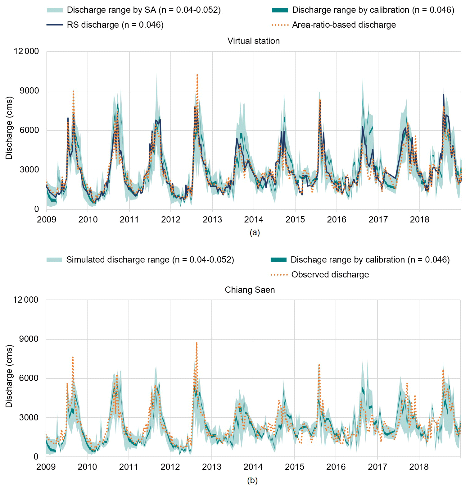
Figure 8 Simulated discharge at the virtual station used for calibration (a) and at Chiang Saen station (used for validation) (b). The dark green band is the variability range of simulated discharge corresponding to the 12 parameterizations produced by the multi-objective calibration, while the light green band corresponds to the 40 parameterizations selected from the sensitivity analysis. The dark blue line is the remotely sensed discharge at the virtual station with n=0.046. In panel (a), the dotted orange line is the discharge at the virtual station scaled from the observed discharge at Chiang Saen. In panel (b), the orange line is the observed discharge at Chiang Saen. The unit “cms” on the y axes represents cubic meters per second.

In Fig. 8b, we report the performance of the model validation at Chiang Saen station. The variability range of the simulated discharge corresponding to the 12 selected parameterizations (dark green band) is much narrower than that of the 40 parameterizations selected through the sensitivity analysis (light green band). The new envelope of variability is also in good agreement with the observed discharge at Chiang Saen station (dotted orange line). The performance metrics of the 12 selected parameterizations show only a small decay when compared against those achieved at the virtual station: NSE, TRMSE, MSDE, and ROCE within the [0.594, 0.616], [3.891, 3.935], [1 057 966, 1 071 282], and [0.169, 0.195] ranges, respectively. (The detailed performance of each parameterization is provided in Table S4.) We note that similar results are achieved by selecting all parameterizations belonging to the Pareto front (58 parameterizations), as shown in Fig. S4 and Tables S5 and S6 in the Supplement. However, visual inspection of the time series in Fig. 8b shows some discrepancies in the time to peak of the discharge at Chiang Saen (e.g., in 2014 and 2017). These discrepancies could be due to different factors, including, as already mentioned above, errors in the precipitation data (Kabir et al., 2022). It should also be noted that the comparison of the discharge at Chiang Saen is our validation; we indeed calibrated our model with remotely sensed discharge at the virtual station. However, overall, the fit to observed discharge at Chiang Saen is a remarkable if we consider that the model was calibrated purely with remotely sensed data at the virtual station and that no gauged discharge data were used for calibration.

Finally, we looked at the parameter values in the 12 parameterizations selected by the model calibration (Fig. S5a). Interestingly, these 12 parameterizations are all quite similar. On the other hand, the 58 parameterizations corresponding to the Pareto front span over a much larger variability range (Fig. S5b). Moreover, these 58 optimal parameterizations are in good agreement with the parameter ranges identified via sensitivity analysis (Sect. 4.2.2).

5 Discussion and conclusions

Our study contributes an approach to calibrate macroscale hydrological models in poorly gauged and heavily regulated basins. The approach uses satellite data to infer both the discharge data used for model calibration and the reservoir operations included in the hydrological model. Unlike previous studies, our approach uses global sensitivity analysis to avoid the biases that could be introduced when co-calibrating the hydrological model and the rating curve used to reconstruct the discharge data (Lima et al., 2019). This fundamental step also helps us narrow down the uncertainty range for the parameterization of the rating curve in a more justified way. In turn, this step paves the way to a more reliable calibration of the hydrological model.

Looking at the specific results of the sensitivity analysis, there are two important points worth stressing here. First, we show that simultaneously estimating the parameters of the hydrological model and the Manning coefficient (by optimizing a set of model performance metrics) may significantly bias the reconstruction of the discharge values. Different combinations of performance metrics can result in different estimates of river discharge, thereby influencing the parameterization of the hydrological model. We saw, for example, that using the NSE for the joint calibration introduces bias in the Manning coefficient towards producing higher flows. Second, the sensitivity analysis specifically focused on the nine parameters of VIC-Res shows the existence of equifinality, meaning that different parameterizations can yield similar performance in terms of the NSE, TRMSE, MSDE, and ROCE. This equifinality issue is perhaps explained by the fact that we are using only river discharge data for calibration. Previous research (Wagener and Pianosi, 2019; Yeste et al., 2020) has shown that a few parameters typically dominate the variability in a given model output (although the parameters that are dominant might vary with the chosen metric). Therefore, one may expect that observations of other hydrological processes, such as evapotranspiration, could help reduce the uncertainty in the model parameters.

Our numerical framework seeks to reduce the pitfalls hidden in model calibration, but, like any other modeling study, is potentially affected by various errors and uncertainties. First, because of the unavailability of gauged rainfall data, we use a gridded product – a common approach for macroscale studies. However, gridded rainfall data inevitably carry errors, especially in regions (like Southeast Asia) where the number of rainfall gauges is limited (Funk et al., 2015; Kabir et al., 2022). Another potential source of uncertainty is the estimation of the river discharge from altimetry water level data (via a rating curve). Our results show that the estimation is reliable; nevertheless, the estimation of river cross-section and the use of water surface slope – needed for constructing the rating curve – could generally contribute to further uncertainty. Specifically, the accuracy of the river cross-section can be affected by the spatial resolution of satellite data (DEM and Landsat images). Furthermore, the DEM, a static “product” captured at a specific time, hardly grasps the evolution of the river cross-section. Moreover, the interpolation of the cross-section below the lowest observed water level may also cause uncertainty. Meanwhile, there could be uncertainty arising from the estimation of water surface slope from a DEM, which captures the water surface slope at the observation time (i.e., February 2000 for the SRTM). A potential solution to this problem could be to calculate the water surface slope from the altimetry water level time series at multiple locations near the virtual station; this is an approach that, of course, is only possible when enough data are available. Looking at the issues of river discharge estimation, a potential game changer is the Surface Water and Ocean Topography (SWOT) NASA satellite mission, launched in December 2022. SWOT will provide river width, water level, and water surface slope for major rivers with an average revisit time of 11 d for the next 3 years (JPL, 2022). This means that we will be able to leverage existing algorithms to estimate river discharge (Gleason and Smith, 2014; Durand et al., 2016; Hagemann et al., 2017) and then inform the implementation of macroscale hydrological models – an area certainly worth additional research. However, we should not forget that model calibration requires time series longer than 3 years. Thus, we could envisage a future in which calibration exercises assimilate multiple discharge data inferred from multiple satellite data.

We note that the approach proposed in this study could be adopted for other basins, although there are a few specific caveats that should be kept in mind. First, the choice of the location for the virtual station (where we construct the river cross-section) should be driven not only by the availability of altimetry data but also by the site topography. In particular, the river banks should not be affected by levees, roads, or other interventions. This is because our approach works best for river banks under natural conditions, as it is possible to infer the relation between river widths and water levels for the portion below the lowest observed water level under the aforementioned conditions. Moreover, the virtual station should be located in a straight river segment with minimal discharge variation due to nearby tributaries and distributaries (both upstream and downstream), a setting in which our approach – based on Manning's equation – works best (Przedwojski et al., 1995). In such locations, the variation in the water surface slope with time is also minimal. Second, if enough data are available, one should consider the option of using altimetry water level time series data at multiple locations (near the virtual station) to estimate the water surface slope. Lastly, we note that our modeling approach is applicable to river basins unaffected by the presence of dams; this simply requires one to switch off the reservoir module in VIC-Res (Dang et al., 2020b).

Looking forward, we should consider expanding frameworks like the one presented here to even more complex modeling environments. For example, a modeling challenge that is often recurring in downstream applications is the presence of multiple human interventions, such as dams, irrigation withdrawals, and groundwater pumping. Understanding how data concerning the representation of all of these processes influence model calibration remains an open question. A similar comment applies to the calibration of multi-basin and global models. Bringing all of these elements together would be a major step towards a more reliable calibration of macroscale hydrological models.