the Creative Commons Attribution 4.0 License.
the Creative Commons Attribution 4.0 License.
 | 30 Jun 2023
The suitability of differentiable, physics-informed machine learning hydrologic models for ungauged regions and climate change impact assessment
Dapeng Feng
Hylke Beck
Kathryn Lawson
As a genre of physics-informed machine learning, differentiable process-based hydrologic models (abbreviated as δ or delta models) with regionalized deep-network-based parameterization pipelines were recently shown to provide daily streamflow prediction performance closely approaching that of state-of-the-art long short-term memory (LSTM) deep networks. Meanwhile, δ models provide a full suite of diagnostic physical variables and guaranteed mass conservation. Here, we ran experiments to test (1) their ability to extrapolate to regions far from streamflow gauges and (2) their ability to make credible predictions of long-term (decadal-scale) change trends. We evaluated the models based on daily hydrograph metrics (Nash–Sutcliffe model efficiency coefficient, etc.) and predicted decadal streamflow trends. For prediction in ungauged basins (PUB; randomly sampled ungauged basins representing spatial interpolation), δ models either approached or surpassed the performance of LSTM in daily hydrograph metrics, depending on the meteorological forcing data used. They presented a comparable trend performance to LSTM for annual mean flow and high flow but worse trends for low flow. For prediction in ungauged regions (PUR; regional holdout test representing spatial extrapolation in a highly data-sparse scenario), δ models surpassed LSTM in daily hydrograph metrics, and their advantages in mean and high flow trends became prominent. In addition, an untrained variable, evapotranspiration, retained good seasonality even for extrapolated cases. The δ models' deep-network-based parameterization pipeline produced parameter fields that maintain remarkably stable spatial patterns even in highly data-scarce scenarios, which explains their robustness. Combined with their interpretability and ability to assimilate multi-source observations, the δ models are strong candidates for regional and global-scale hydrologic simulations and climate change impact assessment.
- Article
(6847 KB) - Full-text XML
- BibTeX
- EndNote


Hydrologic models are essential tools to quantify the spatiotemporal changes in water resources and hazards in both data-dense and data-sparse regions (Hrachowitz et al., 2013). The parameters of hydrologic models are typically calibrated or regionalized for large-scale applications (Beck et al., 2016) which require streamflow data. For global-scale applications, however, models are often uncalibrated (Hattermann et al., 2017; Zaherpour et al., 2018), leading to large predictive uncertainty. Many regions across the world, e.g., parts of South America, Africa, and Asia, suffer from a paucity of publicly available streamflow data (Hannah et al., 2011), which precludes calibration. Yet the water resources in many of these regions face severe pressure due to, among others, population expansion, environmental degradation, climate change (Boretti and Rosa, 2019), and extreme-weather-related disasters, e.g., floods (Ray et al., 2019), heat waves, and droughts. Therefore, it is important to better quantify the impacts of these pressures in these regions (Sivapalan, 2003) and estimate changes in the future water cycle.
There has been a surge of interest in deep learning (DL) models such as long short-term memory (LSTM) networks in hydrology due to their high predictive performance, yet DL is not without limitations. LSTMs have made tremendous progress in the accuracy of predicting a wide variety of variables, including soil moisture (Fang et al., 2017; Liu et al., 2022; O and Orth, 2021), streamflow (Feng et al., 2020, 2021; Kratzert et al., 2019a), stream temperature (Qiu et al., 2021; Rahmani et al., 2021b), and dissolved oxygen (Kim et al., 2021; Zhi et al., 2021), among others (Shen, 2018; Shen and Lawson, 2021). DL is able to harness the synergy between data points and thus thrives in a big data environment (Fang et al., 2022; Kratzert et al., 2019a; Tsai et al., 2021). However, DL models are still difficult to interpret and do not predict variables without first having extensive observations to enable model training. In addition, it is challenging to answer specific scientific questions using DL models, e.g., what is the relationship between variable soil moisture and runoff?, as the LSTM's internal relationships may not be straightforwardly interpretable by humans.
Large-scale predictions for ungauged basins (PUB; Fig. 1a) or ungauged regions (PUR; Fig. 1b) challenge the ability of a model and its parameterization schemes to generalize in space. For both kinds of tests, regionalized LSTM models hold the performance record on daily hydrograph metrics (Feng et al., 2021; Kratzert et al., 2019a). While no clear definition has been universally given for PUB, these PUB tests are typically conducted by randomly holding out basins for testing. As such, PUB can be considered spatial “interpolation”, as there will always be training gauges surrounding the test basins (Fig. 1a). While the LSTM's performance declines from temporal to PUB tests, it obtains better results than established process-based models calibrated on the test basins (Feng et al., 2021; Kratzert et al., 2019a). However, it is uncertain if the process-based models' poorer performance is simply due to structural deficiencies and if they would experience similar declines for PUB. Stepping up in difficulty, prediction for ungauged regions (PUR) refers to tests in which a large region's basins are entirely held out of the training dataset and used only for testing (Fig. 1b). As such, the PUR scenario better represents the case of spatial “extrapolation” encountered in real global hydrologic assessment (Feng et al., 2021). For PUR, the LSTM's performance further declines significantly (Feng et al., 2021). No systematic PUR tests have been done for process-based models, however, perhaps because there has been a serious underappreciation of the difference between PUB and PUR and the risk of model failures due to large data gaps.
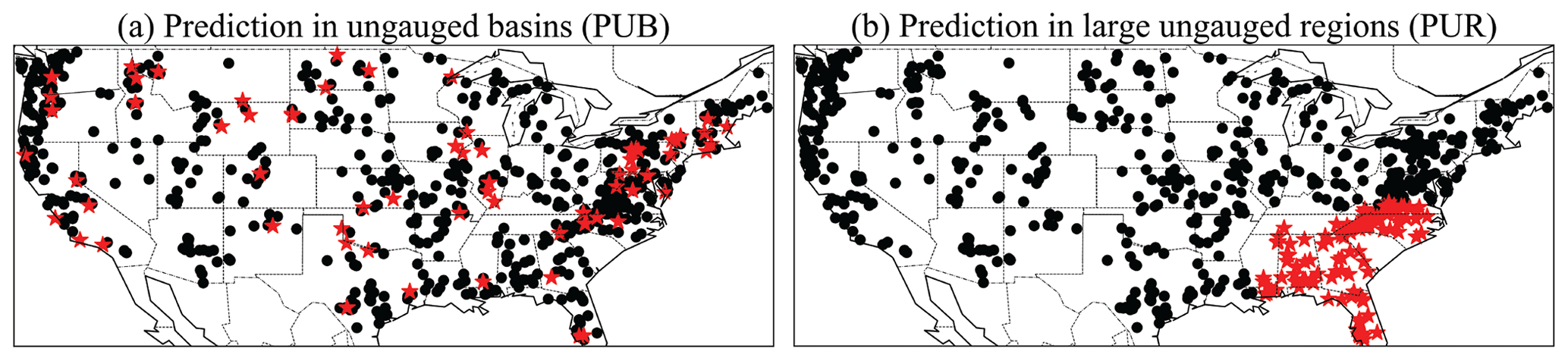
Figure 1A comparison of spatial generalization tests. (a) Prediction in ungauged basins (PUB). (b) Prediction in ungauged regions (PUR) tests. The black dots are the training basins, while the red stars are the test basins for one fold. In this study, we conducted cross-validation to obtain the spatial out-of-sample predictions for basins in the CAMELS dataset.
Recently, a new class of models adopting differentiable programming (a computing paradigm in which the gradient of each operation is tracked; Baydin et al., 2018) has shown great promise (Innes et al., 2019; Tsai et al., 2021). Differentiable modeling is a genre of physics-informed machine learning (or scientific machine learning; Baker et al., 2019). Regardless of the computational platforms chosen for them, differentiable models mix physical process descriptions with neural networks (NNs); these serve as learnable elements for parts of the model pipeline. The paradigm supports backpropagation and neural-network-style end-to-end training on big data, so no ground-truth data are required for the direct outputs of the neural network. The first demonstration in geosciences was a method we called differentiable parameter learning (dPL), which uses NNs to provide parameterization to process-based models (or their differentiable surrogate models; Tsai et al., 2021). Not only did the work propose a novel large-scale parameterization paradigm, but it also further uncovered the benefits of big data; we gain stronger optimization results, acquire parameters which are more spatially generalizable and physically coherent (in terms of uncalibrated variables), and save orders of magnitude in computational power. Only a framework that can assimilate big data, such as a differentiable one, could fully leverage these benefits. However, dPL is still limited by the presence of imperfect structures in most existing process-based models, and some performance degradation is further introduced when a surrogate model is used. As a result, with a LSTM-based surrogate for the Variable Infiltration Capacity (VIC) hydrologic model, dPL's performance is still lower than that of LSTM (Tsai et al., 2021). One plausible avenue to boosting performance is to append neural networks as a post-processor to the physics-based model (Frame et al., 2021; Jiang et al., 2020), but this is not the path we explore here.
Strikingly, differentiable models that evolved the internal structures of the process-based models with insights from data can be elevated to approach the performance level of state-of-the-art LSTM models without post-processors (Feng et al., 2022a). We obtained a set of differentiable, learnable process-based models, which we call δ models, by updating model structures based on the conceptual hydrologic model HBV. Driven by insights provided by data, we made changes to represent heterogeneity, effects of vegetation and deep water storage, and optionally replaced modules with neural networks. For the same benchmark on the Catchment Attributes and Meteorology for Large-sample Studies (CAMELS) dataset (Addor et al., 2017; Newman et al., 2014), we obtained a median Nash–Sutcliffe efficiency (NSE) of 0.71 for the North American Land Data Assimilation System (NLDAS) forcing data, which is already very similar to LSTM (0.72). Furthermore, we can now output diagnostic physical fluxes and states such as baseflow, evapotranspiration, water storage, and soil moisture. Differentiable models can thus trade a rather small level of performance to gain a full suite of physical variables, process clarity, and the possibility of learning science from data.
There are two perspectives with which we can view δ models, namely that they can be regarded as deep networks whose learnable functional space is restricted to the subspace permitted by the process-based backbone or they can be viewed as process-based models with learnable and adaptable components provided by NNs. The flow of information from inputs to outputs is regulated. For example, in the setup in Feng et al. (2022a), the parameterization network can only influence the groundwater flow process via influencing the parameters (but not the flux calculation itself). It does not allow information mixing at all calculation steps (as opposed to LSTM, in which most steps are dense matrix multiplications that mix information between different channels). As another example, because mass balance is observed, a parameter leading to larger annual mean evapotranspiration will necessarily reduce long-term streamflow output. Mass balance is the primary connective tissue between different hydrologic stores and fluxes. These important constraints can lead to tradeoffs between processes if there are errors with inputs like precipitation but impose a stronger constraint on the overall behavior of the model. Nevertheless, the work in Feng et al. (2022a) was conducted only for temporal tests (training on some basins and testing on those same basins but for a different time period) and not for PUB or PUR, which may show a different picture. For these new types of models, their generalizability under varied data density scenarios is highly uncertain. Before we use those models for the purpose of learning knowledge, we seek to understand their ability to generalize.
Our main research question in this paper is whether differentiable process-based models can generalize well in space and provide reliable large-scale hydrologic estimates in data-scarce regions. Our hypothesis is that, since the differentiable models have stronger structural constraints, they should exhibit some advantages in extrapolation compared to both LSTM and existing process-based models. An implicit hypothesis is that the relationships learned by the parameterization component are general, so they can be transferred to untrained regions. If these hypotheses are true, it would make this category of models appropriate for global hydrologic modeling. Since δ models have similar performance to LSTM in temporal tests, they represent a chance to truly test the value of model structures and the impact of extrapolation. In this paper, we designed both PUB and PUR experiments. Furthermore, apart from typical metrics calculated on the daily hydrographs, we also evaluated the simulated trends of mean annual flow and different flow regimes, which are critical aspects for climate change impact assessments but had not previously been adequately assessed.
2.1 Differentiable models
As an overview, a differentiable model implements a process-based model as an evolvable backbone on a differentiable computing platform such as PyTorch, TensorFlow, JAX, or Julia and uses intermingled neural networks (NNs) to provide parameterization (meaning a way to infer parameters for the model using raw information) or process enhancement. In our setup, the parameterization and processes are learned from all the available data using a whole-domain loss function, therefore supporting regionalized PUB applications and even out-of-training-region (PUR) applications. For the process-based backbone, we employed the Hydrologiska Byråns Vattenbalansavdelning (HBV) model (Aghakouchak and Habib, 2010; Beck et al., 2020b; Bergström, 1976, 1992; Seibert and Vis, 2012), a relatively simple, bucket-type conceptual hydrologic model. HBV has state variables like snow storage, soil water, and subsurface storage and can simulate flux variables like evapotranspiration (ET), recharge, surface runoff, shallow subsurface flow, and groundwater flow. The parameters of HBV are learned from basin characteristics by a DL network (gA, an LSTM unit in Fig. 2) just as in dPL. Here, we made two changes to the HBV structure. The first modification was to increase the number of parallel storage components of the HBV model (16 used here) to represent the heterogeneity within basins. The state and flux variables were calculated as the average of different components, and the parameters of all of these components were learned by the neural network gA. The second modification was that, for some tested versions of the model, we turned some static parameters of HBV into time-dependent parameters with a different value for each day (we call this dynamic parameterization or DP). For example, we set the runoff curve shape coefficient parameter to be time-dependent (βt), as explained in Appendix A. The dynamic parameters are also learned by the neural network gA from basin characteristics and climate forcings (Fig. 2). More details about differentiable models can be found in our previous study (Feng et al., 2022a).
2.2 Comparison models
We compared the performance of δ models with a purely data-driven LSTM streamflow model for spatially out-of-sample predictions. The regionalized LSTM model was based on Feng et al. (2020), taking meteorological forcings and basin attributes (detailed below) as inputs. The hyperparameters of both LSTM and δ models were manually tuned in the previous studies and retained in this study. The loss function was calculated as root mean square error (RMSE) for a minibatch of basins with a 1-year look-back period, but across many iterations, the training process will allow the model to go through the entire training dataset. For the δ models, as in Feng et al. (2022a), the RMSE was calculated on both the unnormalized predictions and transformed predictions to improve low-flow representation, and a loss with a two-part weighted combination was used. For the LSTM streamflow model, the RMSE was calculated on the normalized predictions, since the transformation to represent low flow had already been applied in the data preprocessing. Deep learning models need to be trained on minibatches, which are collections of training instances running through the model in parallel, to be followed by a parameter update operation. In our case, a minibatch is composed of 100 training instances, each of which contains 2 consecutive years' worth of meteorological forcings randomly selected from the whole training period for one basin. The first year was used as a warmup period, so the loss was only calculated on the second year of simulation. The model ran on this minibatch, the errors were calculated as a loss value, and then an update of the weights was applied using gradient descent. We also used streamflow simulations from the multiscale parameter regionalization (MPR) scheme (Samaniego et al., 2010) applied to the mHM hydrologic model (Rakovec et al., 2019) to represent a traditional regionalized hydrologic model, but only the temporal test (training and testing in same basins but different time periods) is available for this model.
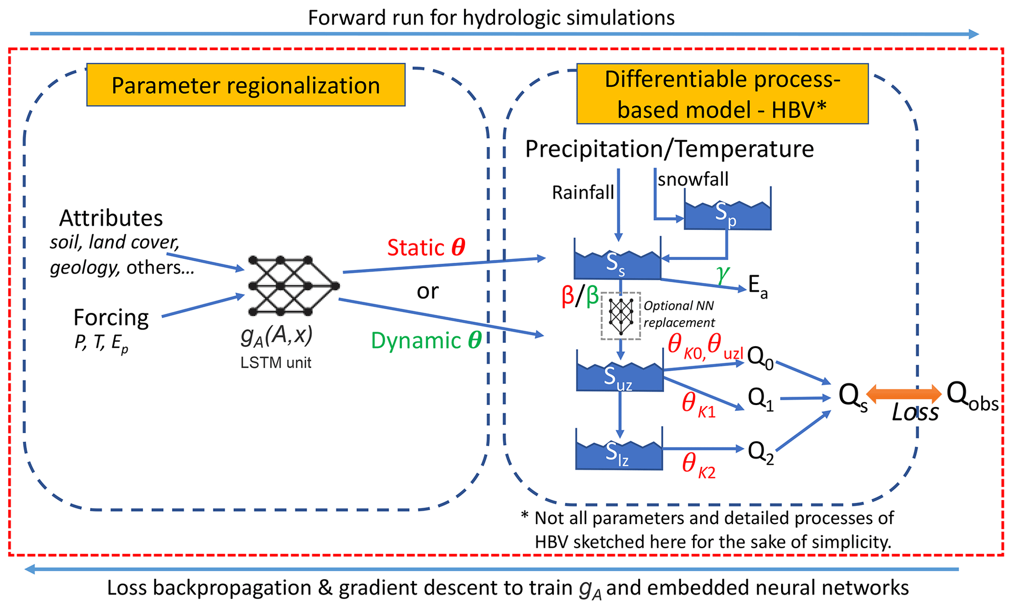
Figure 2The flow diagram of δ models with HBV as the backbone (edited from Feng et al., 2022a). The LSTM unit estimates the parameters for the differentiable HBV model, which has snow, evapotranspiration, surface runoff, shallow subsurface, and deep groundwater reservoirs. Outflows are released from different compartments, using a linear formula with proportionality parameters (θk's). gA is the parameterization network with dynamic input forcing x and static input attributes A. The buckets represent mass storage states (S's); θ, β, and γ refer to all HBV parameters. The model referred to simply as δ has static parameters (red font). The model referred to as δ(βt, γt) sets γ and β as time-dependent parameters (green font), with a new value each day. We only show the original HBV with one set of storage component as illustration, while we use 16 parallel storage components in δ models. The state and flux variables were calculated as the average of different components, and the parameters of all these components were learned by the neural network gA. Importantly, there are no intermediate target variables to supervise the neural networks – the whole framework is trained on streamflow as the only focus of the loss function in an end-to-end fashion. For simplicity, we did not use the optional NN replacement in this study, but the high performance was retained. Note that P is for precipitation, T is for temperature, Ep is for potential evapotranspiration, Q0 is for quick flow, Q1 is for shallow subsurface flow, Q2 is for baseflow, Ea is for actual evapotranspiration, Sp is for snowpack water storage, Ss is for soil water storage, Suz is for upper subsurface zone water storage, Slz is for lower subsurface zone water storage, θuzl is for upper subsurface threshold for quick flow, β is for the shape coefficient of the runoff relationship, and γ is for the newly added dynamic shape coefficient of the evapotranspiration relationship.
2.3 Data
We used the CAMELS dataset (Addor et al., 2017; Newman et al., 2014), which includes 671 basins across the contiguous United States (CONUS) to run the experiments. The Maurer et al. (2002; hereafter denoted as Maurer) meteorological forcing data were selected from the three forcings available in CAMELS to be comparable with existing regionalized model results. We also ran experiments with Daymet (Thornton et al., 2020) forcings to show the impacts of different forcing data. To train regionalized models for dPL and LSTM, we used 35 attributes, as shown in Table A1 in Appendix A. For the LSTM streamflow model, the attribute data were directly concatenated with the forcings and provided as inputs. With the δ models, the neural network gA receives attributes and historical forcing data as inputs and then outputs parameters for the evolved HBV model. The LSTM model takes five forcing variables including precipitation, temperature, solar radiation, vapor pressure, and day length, while the HBV model only takes precipitation (P), temperature (T), and potential evapotranspiration (Ep). We used the temperature-based Hargreaves (1994) method to calculate Ep and the daily Maurer minimum and maximum temperatures for CAMELS basins were acquired from Kratzert (2019a). The training target for all the models was streamflow observations. We trained all models on all 671 basins in CAMELS and reported the test performance on a widely used 531-basin subset, which excludes some basins due to unclear watershed boundaries (Newman et al., 2017). The results of some previous regionalized modeling efforts are also used to provide benchmark context (Kratzert et al., 2019b; Rakovec et al., 2019). For the comparison of evapotranspiration, we used a product derived from the Moderate Resolution Imaging Spectroradiometer (MODIS) satellite (Mu et al., 2011; Running et al., 2017). This ET product served as a completely independent, uncalibrated validation for the evapotranspiration simulated by the differentiable HBV models.
2.4 PUB and PUR experiments
As mentioned earlier, we designed two sets of experiments to benchmark the models, namely predictions in ungauged basins (PUB) and predictions in large ungauged regions (PUR; illustrated in Fig. 1). For PUB experiments, we randomly divided all the CAMELS basins into 10 groups, trained the models on 9 groups, and tested it on the one group held out. By running this experiment for 10 rounds and changing out the group held out for testing, we can obtain the out-of-sample PUB result for all basins. For the PUR experiment, we divided the whole CONUS into seven continuous regions (as shown in Fig. B1 in Appendix B), trained the model on six regions, and tested it on the holdout region. We ran the experiment seven times so that each region could serve as the test region once. The study period was from 1 October 1989 to 30 September 1999. These spatial generalization tests were trained and tested in the same time period but for different basins.
From the daily hydrograph, we calculated the Nash–Sutcliffe (NSE; Nash and Sutcliffe, 1970) and Kling–Gupta (KGE; Gupta et al., 2009) model efficiency coefficients as performance metrics. NSE characterizes the variance in the observations explained by the simulation, and KGE accounts for correlation, variability bias, and mean bias. We also reported the percent bias of the top 2 % peak flow range (FHV) and the percent bias of the bottom 30 % low flow range (FLV; Yilmaz et al., 2008), which characterizes peak flows and baseflow, respectively.
We also evaluated the multi-year trend for streamflow values at different percentiles (Q98, Q50, and Q10), in addition to the mean annual flow. Q98, Q50, and Q10 represent the peak flow, median flow, and low flow values, respectively. To this end, for each year we calculated one data point corresponding to a flow percentile. Then, Sen's slope estimator (Sen, 1968) for the trend of that flow percentile was calculated for the 10 years in the test period and compared with the equivalent slope for the observations. Since streamflow records contain missing values, we only considered years with <61 (about 2 months) daily missing values (not necessarily consecutive) for this purpose.
In this section, we first compared LSTM and the differentiable models (and, when available, the traditional regionalized model) for PUB and PUR in terms of both the daily hydrograph metrics (NSE, KGE, FLV, and FHV) and decadal-scale trends. We then attempted to examine why δ models had robust performance and how well they could predict untrained variables (evapotranspiration). We use the term δ models to generically refer to the whole class of differentiable models, presented in this work with evolved HBV, while we use δ, δ(βt) or δ(βt, γt) to refer to particular models with static, one-parameter dynamic, and two-parameter dynamic parameterizations, respectively. The meanings of β and γ are described in Appendix A.
3.1 The randomized PUB test
For the randomized PUB test, which represents the spatial interpolation in a data-dense scenario (Fig. 1a), the δ models approached (under the Maurer forcings) or surpassed (under the Daymet forcings) the performance of the LSTM on the daily hydrograph metrics. Under the Maurer forcings, δ(βt, γt) had a median PUB NSE of 0.64, which is only slightly lower than LSTM (0.65) and considerably higher than MPR + mHM (0.53; this model is in sample – all basins were included in training). When one moves from in-sample prediction to PUB, the performance of all types of models drops, as demonstrated by δ(βt, γt; Fig. 3a). For KGE, δ(βt) and δ(βt, γt) models not only had median values of 0.66 and 0.65, respectively, which were essentially the same as LSTM, but also had a smaller spread (Fig. 3a). The LSTM had lower errors for FLV and FHV than the δ models (Fig. 3a), which is possibly because the LSTM is not subject to physical constraints like mass balances and therefore possesses more flexibility in terms of base and peak flow generation than HBV.
Under the Daymet forcings, δ(βt) and δ(βt, γt) models reached NSE (KGE) median values of 0.68 (0.68) and 0.69 (0.67), respectively, which is surprisingly higher than the LSTM at 0.66 (0.66) (Fig. 3b). Both the LSTM and δ models showed better performance when driven by Daymet forcings, which is consistent with previous studies using different forcings (Feng et al., 2022a; Kratzert et al., 2021), but δ models improved even more noticeably, showing a clear outperformance of the other models. This result suggests that precipitation in the Maurer forcing data may have a larger bias, and as δ models conserve mass and cannot by default apply corrections to the precipitation amounts, they are more heavily impacted by such bias. It is worthwhile to note that the performance shown here is for a PUB test with a higher holdout ratio (lower k fold which means larger gaps for spatial interpolation), which degrades the performance compared to the metrics we reported earlier (Feng et al., 2021). As mentioned earlier, LSTM may potentially learn to correct biases in precipitation (Beck et al., 2020a), but the impact of precipitation bias is under debate (Frame et al., 2023). Overall, the similar performance and smaller spread of the δ models compared to the LSTM are highly encouraging.
In terms of the prediction of decadal trends in ungauged basins, δ models again demonstrated high competitiveness, showing mixed comparisons to LSTM (Fig. 4). Both LSTM and δ models accurately captured the trends in annual mean flow (R2>0.80) and high-flow bands (R2>0.70), but both struggled with low flow Q10 (trend evaluated in the annual 10th percentile flow; R2<0.40). δ(βt, γt) had similar trend performance to LSTM in terms of annual mean flow, median flow Q50, and peak flow Q98, while LSTM had the advantage for low flow, Q10. Overall, just as with LSTM, δ models seem appropriate for long-term trend predictions in the data-dense PUB scenario.
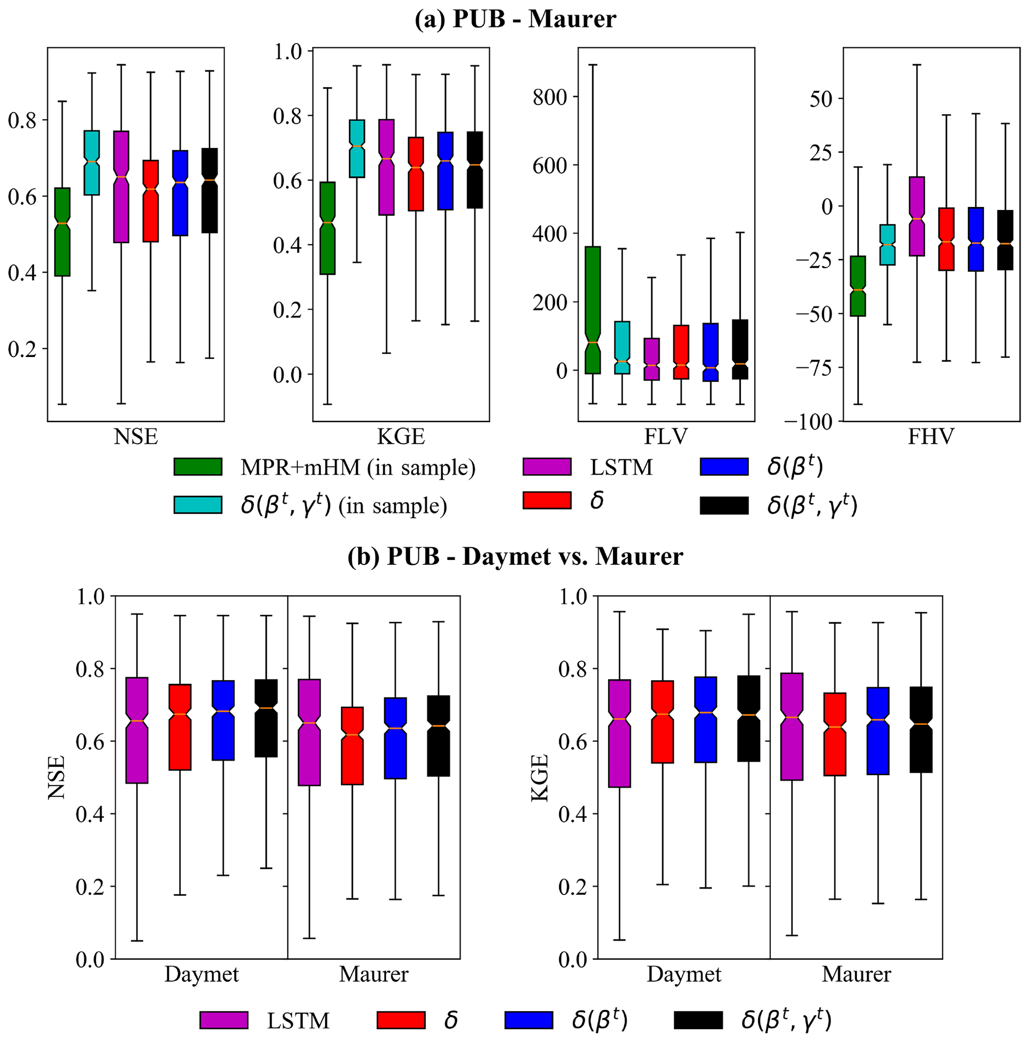
Figure 3Performance of simulated daily hydrographs from the models for (a) the randomized PUB experiment using Maurer meteorological forcing data. (b) Comparison of PUB results using either Maurer or Daymet forcing data. Each box summarizes 531 values (one for each CAMELS basin) obtained as a result of cross-validation. All models except those denoted as “in sample” (which means all sites are included in the training set and thus is at an advantage in testing) were evaluated out-of-sample spatially; i.e., they were trained on some basins and tested on other holdout basins. For MPR + mHM (Rakovec et al., 2019), all test basins were included in the training dataset. NSE is the Nash–Sutcliffe model efficiency coefficient, KGE is the Kling–Gupta efficiency, FLV is the low flow percent bias, and FHV is the high flow percent bias. δ, δ(βt), or δ(βt, γt) refer to the differentiable, learnable HBV models with static, one-parameter dynamic, and two-parameter dynamic parameterizations, respectively. The horizontal line in each box represents the median, and the bottom and top of the box represent the first and third quantiles, respectively, while the whiskers extend to 1.5 times the interquartile range from the first and third quantiles, respectively. The PUB was run in a computationally economic manner to be comparable to other models, while also reducing computational demand; we used only 10 years of training period, did not use an ensemble, and used a lower k fold. When we previously ran the experiments using the same settings as Kratzert et al. (2019a), our LSTM was able to match the PUB performance in their work (Feng et al., 2021).
The challenge with a low flow prediction for all models is probably attributable to multiple factors, including (i) a lack of reliable information on subsurface hydraulic properties which hampers all models. (ii) There is an inherent challenge with baseflow trends, as the magnitude of the Q10 change trends is in the range of −0.5 to 1 m3 s−1 yr−1, while that for the annual mean flow is −2 to 10 m3 s−1 yr−1. Even a small error in absolute terms can result in a large decrease in R2. (iii) The inadequacy of the low flow modules is also challenging because the linear reservoir formulation in the present HBV groundwater modules may not capture the real-world dynamics, while even the LSTM may not have the memory that is long enough to represent a gentle multi-year baseflow trend change. (iv) The greater impact of human activities such as reservoir operations on low flow also needs to be considered (Döll et al., 2009; Suen and Eheart, 2006). (v) Finally, the greater sensitivity of the training loss function to high flows compared to low flows due to the difference in their magnitudes presents another challenge. High flows are direct reflections of recent precipitation events in the basin, while low flows are under large impacts of the geological system.
For completeness, we also evaluated the trends for the temporal tests (models trained and tested on the same basins but in different time periods; Fig. 5). For the temporal test, the model δ's Q98 trends (0.88) are as accurate as those of LSTM for high flows (0.87), but LSTM outperformed δ models for the median and low flows (Q50 and Q10). This test, which excluded the impact of spatial generalization, suggests that the δ models' surface runoff routine has the ability to transform long-term forcing changes into the correct streamflow changes, but the current groundwater module may be suboptimal (or, stated in another way, it loses information). Also, compared to LSTM, δ models are more subject to tradeoffs due to maintaining mass balances and thus could be trained to put more focus on the peaks of the hydrograph while sacrificing the low flow end.
Both LSTM and δ models surpassed MPR + mHM in the temporal test by varying extents for all flow percentiles, which demonstrated the potential from adaptive, learnable models. The MPR + mHM high flow (Q98, R2=0.69) and median flow (Q50, R2=0.63) trends lagged noticeably behind, while the difference in the low flow (Q10, R2=0.24) was smaller. It was previously shown in Feng et al. (2022a; and thus omitted here) that median NSEs of MPR + mHM, δ(βt, γt), and LSTM were 0.53, 0.711, and 0.719, respectively (the first with Maurer forcings, while the other two were with NLDAS forcing data). Compared to the learnable models, MPR + mHM tends to underestimate the wetting trend for the high flow and overestimate the wetting trend for the low flow. The fact that MPR + mHM correctly predicted the annual mean flow trend despite having lower metrics for flow percentiles suggests that it had a decent overall mass balance but might have directed flows through different pathways than δ models. Note that the temporal test is the only comparison that we can carry out with existing regionalized process-based hydrologic models. Common benchmark problems certainly help the community understand the advantages and disadvantages of each model (Shen et al., 2018), and we encourage work towards obtaining PUB or PUR experimental results from existing models, which would facilitate such comparisons.
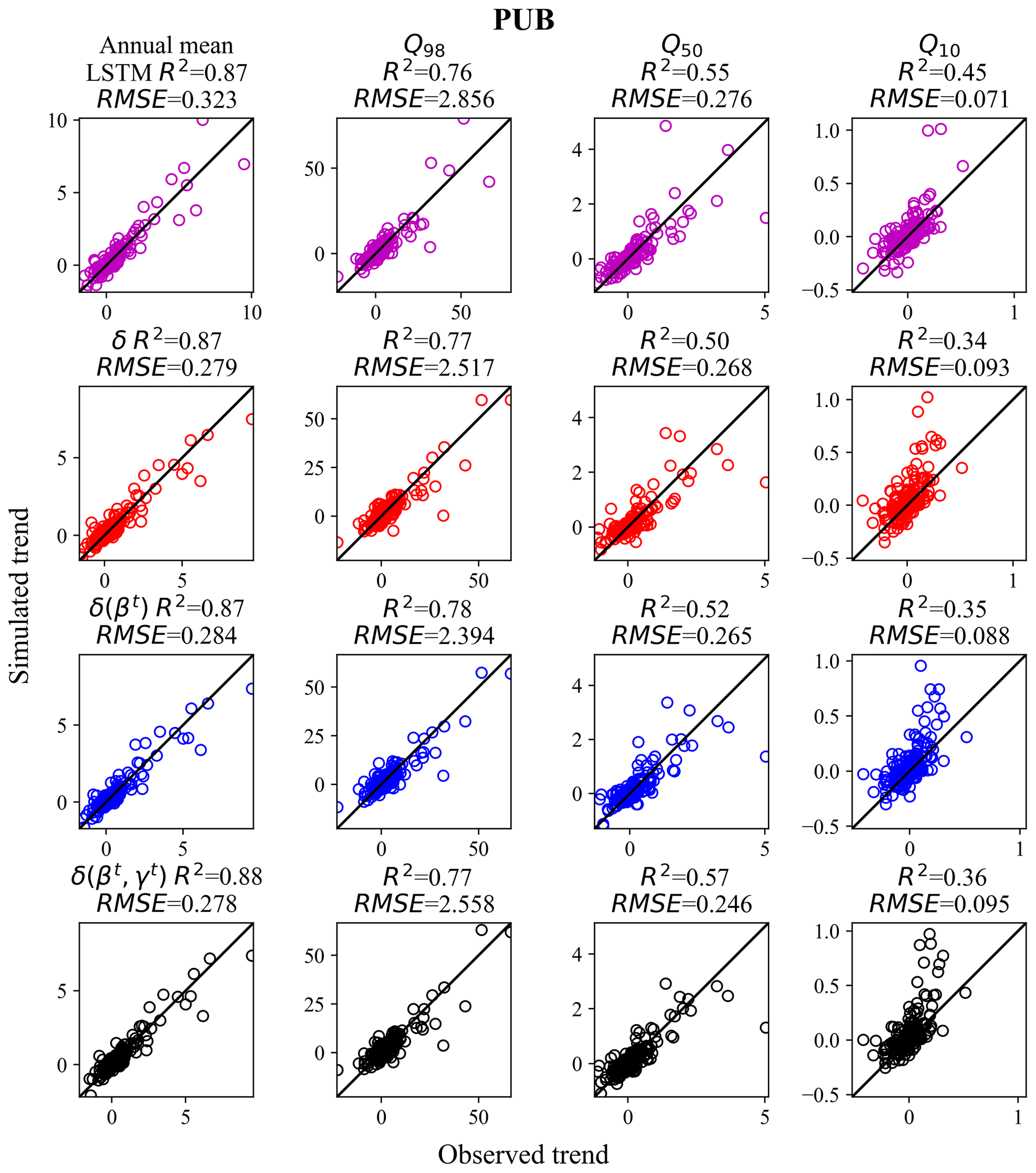
Figure 4Decadal trends (m3 s−1 yr−1) of streamflow for different flow percentiles for the randomized PUB cross-validation experiment (using Maurer forcing data), as compared to the observed trends. Chart columns are organized by flow percentile. Q10, Q50, and Q98 mean that the trends were evaluated in the annual 10th, 50th, and 98th percentile flows, respectively (or more simply, low, median, and high flows). Chart rows are organized by model, and results for LSTM are shown in pink, results for δ are in red, δ(βt) are in blue, and δ(βt, γt) are in black. δ, δ(βt), or δ(βt, γt) refer to the differentiable, learnable HBV models with static, one-parameter dynamic, and two-parameter dynamic parameterizations, respectively. For each flow percentile, a corresponding value was extracted from each year's daily data, and Sen's slope was estimated and evaluated between hydrologic years 1989 and 1999.
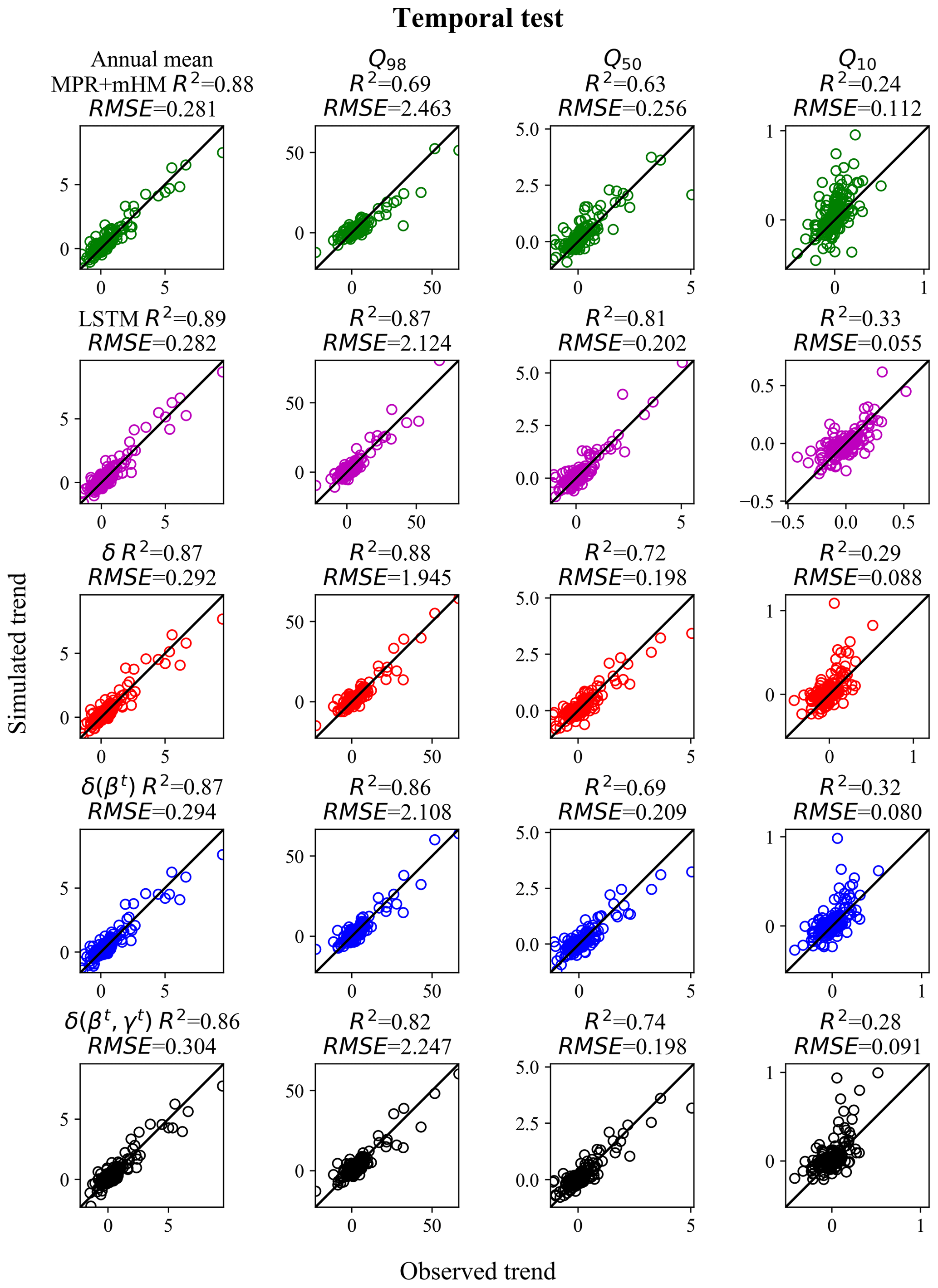
Figure 5Observed vs. simulated decadal trends (m3 s−1 yr−1) of streamflow for the temporal test for 447 basins where MPR + mHM has predictions (all models trained with Maurer forcing data from 1999 to 2008 and tested from 1989 to 1999 of hydrologic years on the same basins). We could only compare the trends with an existing process-based model with a parameter regionalization scheme on the temporal test because we did not have their systematic PUB results on the same dataset. Chart columns are organized by flow percentile. Q10, Q50, and Q98 mean that the trends were evaluated in the annual 10th, 50th, and 98th percentile flows, respectively (or more simply, low, median, and high flows). Chart rows are organized by model, and results for MPR + mHM are shown in green, LSTM are in pink, results for δ are in red, δ(βt) are in blue, and δ(βt, γt) are in black. δ, δ(βt), or δ(βt, γt) refer to the differentiable, learnable HBV models with static, one-parameter dynamic, and two-parameter dynamic parameterizations, respectively. For each flow percentile, a corresponding value was extracted from each year's daily data, and Sen's slope was estimated and evaluated between hydrologic years 1989 and 1999.
3.2 The region-based PUR test
For the regional holdout test (PUR), surprisingly, δ models noticeably outperformed LSTM in most of the daily hydrograph metrics (KGE, NSE, and FHV) and again had smaller spreads in these metrics (Fig. 6). The LSTM's performance dropped substantially from PUB to PUR, while the performance for δ models dropped less. Under Maurer forcings, the median NSE values for LSTM, δ, and δ(βt, γt) models were 0.55, 0.56, and 0.59, respectively, and the corresponding KGE values were 0.52, 0.59, and 0.61, respectively. The performance gap between LSTM and δ models was larger under Daymet forcings. The LSTM had a minor performance gain when using Daymet forcings, while the δ models had significant performance improvements. The median NSE (KGE) values for LSTM, δ, and δ(βt, γt) models were 0.55 (0.51), 0.60 (0.61) and 0.62 (0.63), respectively. We see that for the low flow dynamics, δ(βt) had a slightly smaller low flow bias (FLV). For high flow, δ models still had negative biases, but they were smaller than those of LSTM (Fig. 6a).
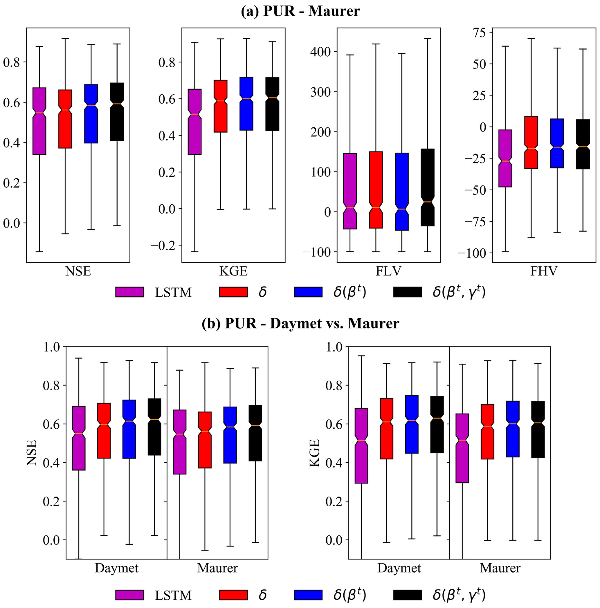
Figure 6Same as Fig. 3 but for the regional holdout (PUR) test. Performance of simulated daily hydrographs from the models for (a) the regionalized PUR experiment using Maurer meteorological forcing data. (b) Comparison of PUR results using either Maurer or Daymet forcing data. Each box summarizes the metrics of 531 basins obtained in a regional cross-validation fashion. We see the clear outperformance of LSTM by the δ models for these daily hydrograph metrics (NSE, KGE, and FHV).
With the exception of regions 4 and 5, the δ models have advantages over LSTM in nearly all other PUR regions, suggesting that the benefits of physical structure for extrapolation are robust in most situations (Fig. B2). Region 5 is the Southern Great Plains, with frequent flash floods and karst geology, and both types of models performed equally poorly. δ(βt, γt) showed significant performance advantages in regions 3, 6, and 7. It is unclear why larger differences exist in these regions rather than others. We surmise that these regions feature large diversity in the landscape (as opposed to regions 2, 4, and 5, which are more homogeneous forest or prairie on the Great Plains), which, when missing from the training data, could cause a data-driven model like LSTM to incur large errors. Meanwhile, all the models achieve their best PUR results in region 1 (northeast) and region 7 (northwest), with NSE/KGE medians larger than or close to 0.6 (Fig. B2), which are consistent with our previous PUR study using LSTM (Feng et al., 2021). We also observe that both LSTM and evolved HBV models have difficulty with accurately characterizing hydrologic processes in arid basins as shown by regions 4 and 5 in the middle CONUS.
The decadal flow trends showed a stronger contrast – while the LSTM's trend metrics declined noticeably from PUB to PUR, the δ models' trend accuracy barely budged (Fig. 7). For the annual mean flow, the points for δ(βt, γt) tightly surrounded the ideal 1:1 line and correctly captured the basins with strong wetting trends toward the higher end of the plot. In contrast, LSTM showed an underestimation bias and a tendency to plateau for the wetting basins. The same pattern is obvious for the high flow (Q98). We previously also noticed such a flattening tendency for LSTM in multi-year soil moisture trend prediction (see Fig. 9 in Fang et al., 2019), although there the model was trained on satellite data, which could also have played a role. The LSTM R2 for annual mean discharge dropped from 0.87 for PUB to 0.64 for PUR, but R2 remained at 0.88 for δ(βt, γt). The LSTM R2 for high flow (Q98) trends dropped significantly, from 0.76 for PUB to 0.27 for PUR, whereas this metric remained around 0.77 for the δ models. The results highlight the δ models' robust ability to generalize in space, possibly due to the simple physics built into the model.
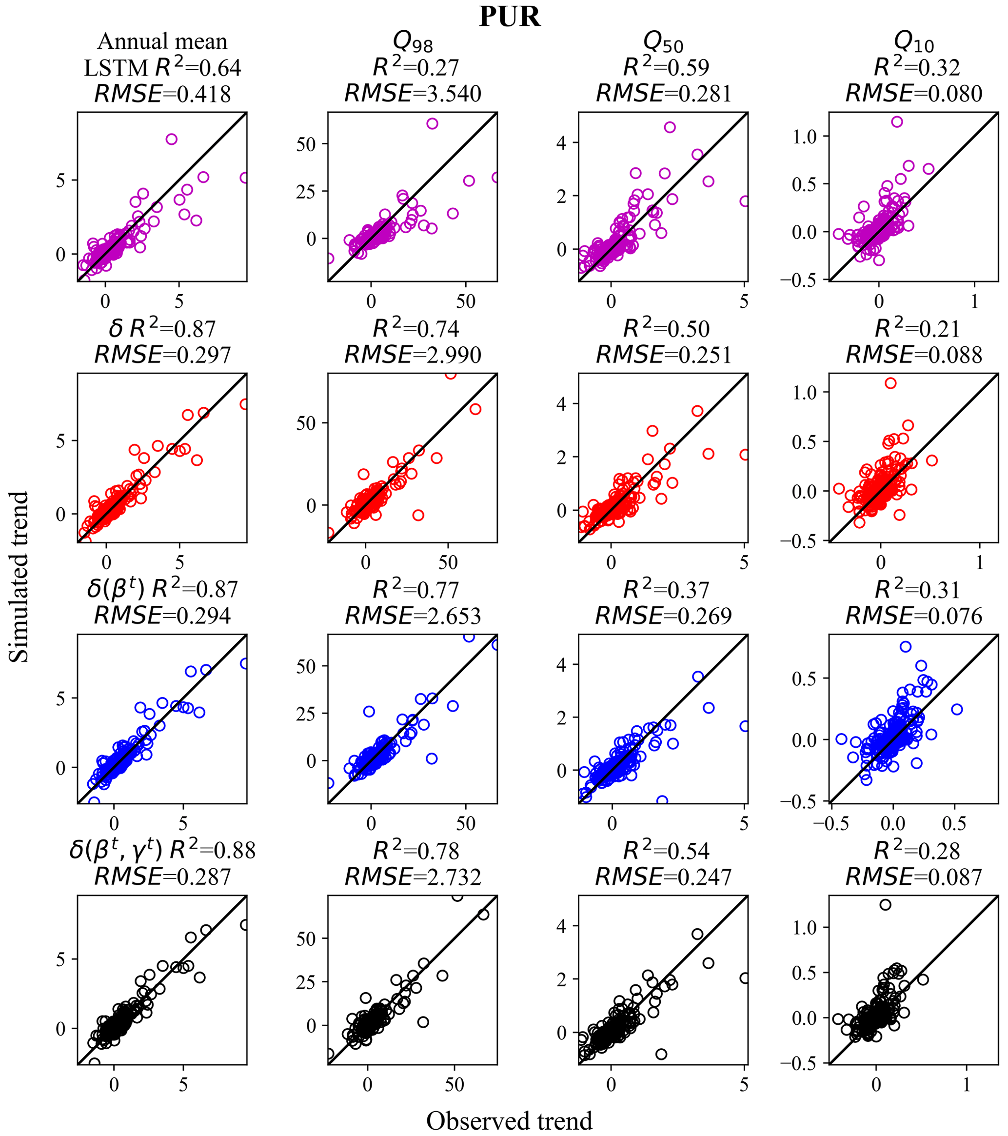
Figure 7Same as Fig. 4 but for the regional holdout (PUR) experiment (using Maurer forcing data). δ models outperformed LSTM for the decadal trends (m3 s−1 yr−1) of the mean annual flow and the high flow regime. Chart columns are organized by flow percentile. Q10, Q50, and Q98 mean the trends were evaluated in the annual 10th, 50th, and 98th percentile flows, respectively (or more simply, low, median, and high flows). Chart rows are organized by model, and results for LSTM are shown in pink, results for δ are in red, δ(βt) are in blue, and δ(βt, γt) are in black. δ, δ(βt) or δ(βt, γt) refer to the differentiable, learnable HBV models with static, one-parameter dynamic, and two-parameter dynamic parameterizations, respectively. For each flow percentile, a corresponding value was extracted from each year's daily data and Sen's slope was estimated and evaluated between hydrologic years 1989 and 1999.
What makes δ models more robust than LSTM for PUR, especially in terms of high flow and mean annual flow? As indicated earlier, δ models can be considered to be machine learning models that are restricted to a subspace allowable by the backbone structure. There are two structural constraints, namely that (i) the static attributes can only influence the model via fixed interfaces (model parameters) and (ii) the whole system can only simulate flow as permitted by the backbone model of HBV. Hence, we can force the parameterization to learn a simpler and more generic mapping relationship, and when it succeeds, the relationship could be more transferable than that from LSTM, which mixes information from all variables in most steps.
The δ model-based parameter maps reveal that the in-sample, PUB, and PUR experiments all produced similar overall parameter patterns (see Fig. 8; for PUB in Fig. 8b and PUR in Fig. 8c, these parameters were generated when the basins were used as the test basins and excluded from training). Between in-sample (temporal) and PUB tests, most of the points had similar colors, except for a few isolated basins (e.g., some basins in New Mexico). Between PUB and PUR, there were more regional differences (e.g., in the Dakotas, North Carolina, and Florida), but the overall CONUS-scale patterns were still similar. Recall that (i) these parameters were estimated by the parameter network gA, which was trained on streamflow, and there are no ground-truth values for the parameters, and (ii) in the PUR experiments, a large region was held out. Despite these strong perturbations to the training data, such parameter stability under PUB and PUR is impressive. This stability is part of the reason for the mild performance drop under PUR. Had we used a basin-by-basin parameter calibration approach, the parameter values would have been much more stochastic and interspersed (similar to Fig. 5b in Tsai et al., 2021).
We note that δ models found advantages in the annual mean flow and high flow regimes rather than the low flow regime for the PUR test. As described above, we attribute the advantage in high flow to learning a more generalizable mapping between raw attributes and runoff parameters. For the low flow component, we hypothesize that the δ models' groundwater module, which is inherited from HBV and based on a simple linear reservoir, cannot adequately represent long-term groundwater storage changes. This part of the model will likely require additional structural changes, e.g., by adopting nonlinearity (Seibert and Vis, 2012) or considering feedback between layers in the groundwater modules. Furthermore, due to the guaranteed mass balance, the δ models face more tension (or tradeoffs) between the low and high flow regimes during training. The peak flow part tends to receive more attention due to its larger values. Because pure LSTM models do not guarantee the conservation of mass, they are subject to fewer tradeoffs and are more likely to capture both high and low flows. We believe future work can further improve the groundwater representation by considering better topographic distributions.
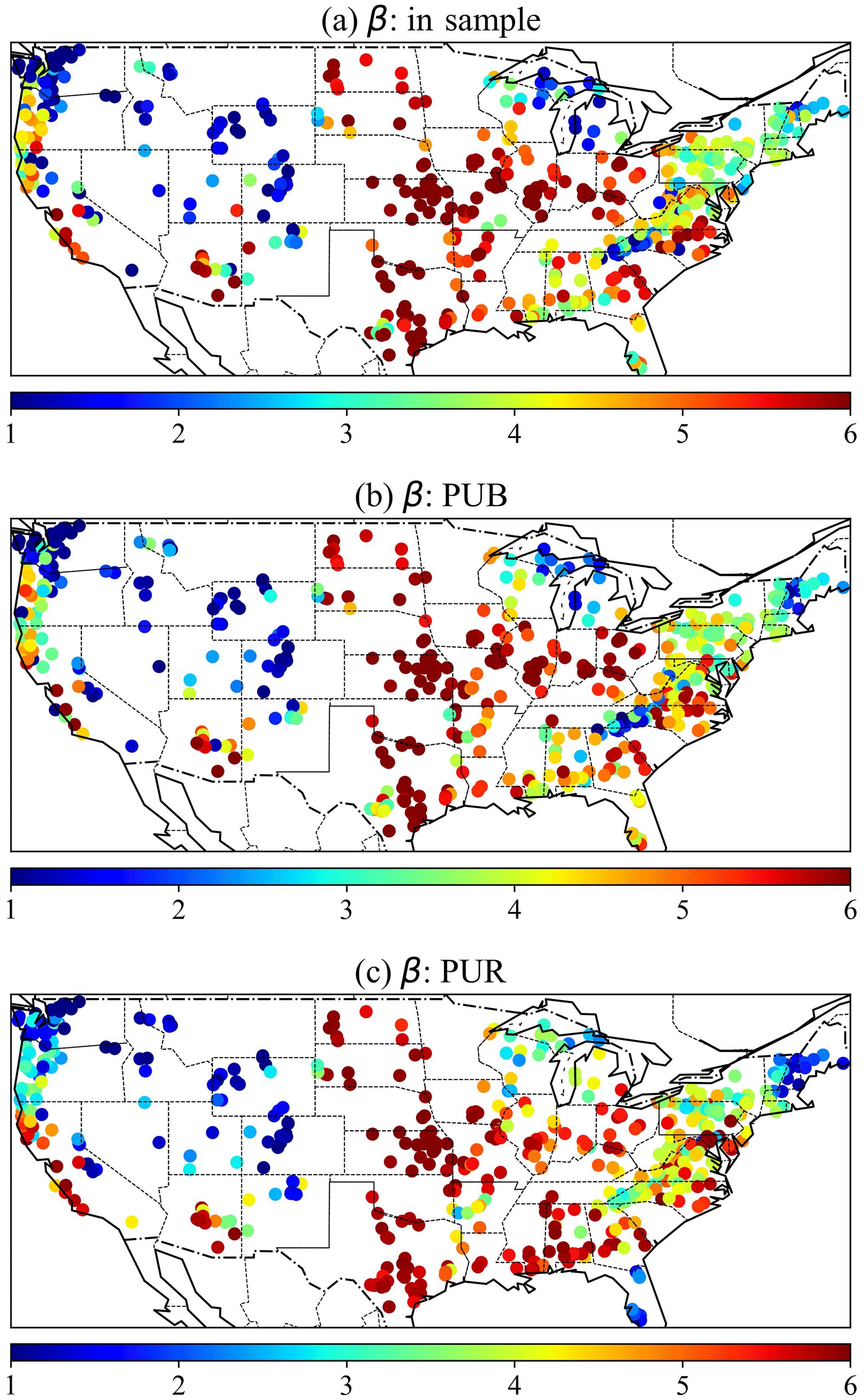
Figure 8Parameter maps for the β parameter of the HBV model for (a) the in-sample temporal test, (b) PUB, and (c) PUR. For PUB and PUR, all the parameters were produced from cross-validation experiments when the sites were used as test sites and were not included in the training data. With other conditions being the same, higher β yields less runoff, but other parameters such as the maximum soil water storage also influence runoff. For simplicity, these parameters were the outputs of the parameterization network (gA) in the δ models without dynamical parameterization. We show the maps of the mean parameter value of multiple components here. Again, there is no ground truth parameter to supervise gA.
3.3 The impacts of extrapolation on evapotranspiration
Spatial interpolation and extrapolation seemed to have a moderate impact on evapotranspiration (ET) seasonality and a muted impact on annual mean ET (Fig. 9). For δ(γt, βt), from temporal tests to PUB and then PUR, the median correlation and RMSE between simulated ET and 8 d integrated ET from the MODIS satellite product did not vary much, around 0.84 and 6.4 mm per 8 d, respectively. The impact of extrapolation on ET was more muted compared to streamflow. Understandably, ET is controlled by the energy input and physics-based calculations, and thus the models cannot deviate too much from each other. It is worthwhile to note that we only trained δ models on streamflow and used MODIS ET as an independent data source for verification, while the LSTM trained on streamflow is unable to output ET or other physical variables on which it has not been explicitly trained.
Moreover, the dynamic parameterization (DP) models, δ(γt, βt) and δ(βt), were better than static parameter models in all comparable cases (temporal test, PUB, or PUR). The decline due to spatial interpolation or extrapolation was minimal. Even for the most adverse case, i.e., PUR, δ(γt, βt) provided a high-quality ET seasonality as compared to MODIS (median correlation of 0.84) and low RMSE. It appears that DP indeed captured missing dynamics in data, possibly attributable to long-term water storage and vegetation dynamics and presented better models for the right reasons.
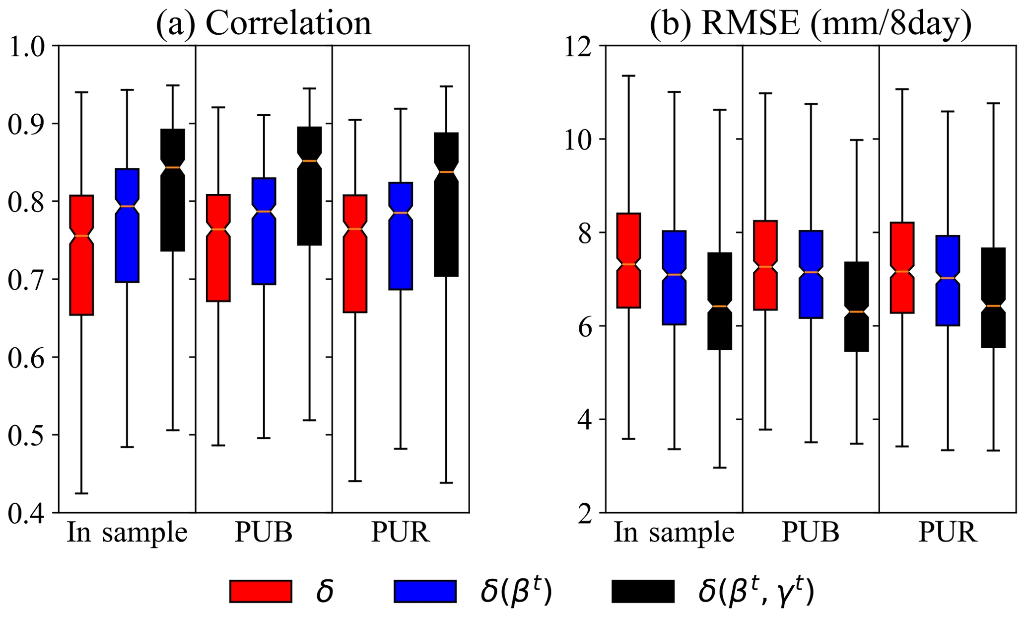
Figure 9Comparison of the agreement of simulated ET and the MODIS satellite product for different models under the temporal test (in sample), PUB, and PUR scenarios using two different metrics, namely (a) correlation and (b) root mean square error (RMSE). All models were trained only with streamflow as the target. LSTM is not shown, as it is unable to output physical variables on which it has not been explicitly trained.
3.4 Further discussion and future work
For all cases tested, and for both streamflow and ET, the models with dynamical parameterization (DP), δ(γt, βt), had better generalization than the δ models without DP. In theory, the models with DP have more flexibility, and correspondingly, we had expected DP models to be more overfitted in some cases. However, the results showed δ(γt, βt) to be comparable or slightly better in most cases (either trends or NSE/KGE) than δ and δ(βt); thus, the expected overfitting did not occur. Although the LSTM-based parameterization unit gA has a large amount of weight, it can only influence the computation through restricted interfaces (the HBV parameters). In contrast, the full LSTM model we tested allows attributes to influence all steps of the calculations. The fact that δ(γt, βt) was more generalizable also suggests that whether the model will overfit or not depends on the way the computation is regulated, rather than simply the number of weights. It seems DP may have enabled the learning of some true processes that are missing from HBV, possibly related to deep soil water storage and/or vegetation dynamics (Feng et al., 2022a).
While not directly tested here, it is easy to imagine that in the future we can constrain the δ models using multiple sources of observations. So far, the simulation quality seems consistent between streamflow and ET, e.g., δ(γt, βt) is better than δ in streamflow (NSE/KGE) and also ET. This has not always been true traditionally, due to equifinality (Beven, 2006), and it means a better conditioning of one of these variables could have positive impacts on other variables. Over the globe, while gauged basins are limited, there are many sources of information on soil moisture (ESA, 2022; NSIDC, 2022; Wanders et al., 2014), water storage (Eicker et al., 2014; Landerer et al., 2020), in situ measurements of ET (Christianson, 2022; Velpuri et al., 2013), snow cover (Duethmann et al., 2014), and other measurements that provide additional opportunities for learning from multiple types of data sources, or data sources on different scales (Liu et al., 2022).
This study demonstrated how well the novel differentiable models can generalize in space with other regionalized methods providing context. To ensure comparability across different models, we have chosen the same setups, e.g., meteorological forcings, training and testing samples and periods, and random seeds, rather than configurations that would maximize performance metrics. This work also does not invalidate deep learning models as valuable tools, as LSTM is a critical part of the parameterization pipeline for the differentiable models. The point of differentiable models is to maximally leverage the best attributes of both deep networks (learning capability) and physical models (interpretability). Several strategies can be applied to enhance the pure data-driven LSTM performance, as shown in earlier studies. For example, some auxiliary information like soil moisture can be integrated by a kernel to constrain and enhance the extrapolation (Feng et al., 2021). LSTM models can utilize multiple precipitation inputs simultaneously to gain better performance (Kratzert et al., 2021), which can be more complicated to achieve for models with physical structures. Ensemble-average prediction from different initializations (Kratzert et al., 2019a) or different input options (Feng et al., 2021; Rahmani et al., 2021a) can often lead to higher performance metrics. Here, however, we used a less computationally expensive but comparable setup without these strategies applied, which can certainly be studied in the future.
We used CONUS basins and large regional hold-outs to examine the spatial generalization of different models. PUR is a global issue because many large regions in the world lack consistent streamflow data. We ran experiments over the CONUS in this paper to ensure comparability with previous work and to benchmark on a well-understood dataset. It has been demonstrated that models trained on data-rich continents can be migrated to data-poor continents. Ma et al. (2021) showed that deep learning models may learn generic hydrologic information from data-rich continents and leverage the information to improve predictions in data-poor continents with transfer learning. More recently, Le et al. (2022) examined PUR in global basins for monthly prediction with traditional machine learning methods, and the results demonstrated the difficulties of this issue. In future work, we will establish differentiable models for a large sample of global basins by integrating modern DL and physical representations that have shown promising spatial generalizability and examine their value for accurate daily PUR at the global scale.
We demonstrated the high competitiveness of differentiable, learnable hydrologic models (δ models) for both spatial interpolation (PUB) and extrapolation (PUR). Evidence for such high competitiveness is provided in terms of daily hydrograph metrics, including NSE and KGE, and in terms of decadal-scale trends, which are of particular importance for climate change impact assessments. For the daily hydrograph metrics, the δ models closely approached the LSTM model in the PUB test (while showing less spread) and outperformed the LSTM model in the PUR test. For the decadal-scale trends, the δ models outperformed the LSTM model noticeably in the PUR tests, especially for the annual mean flow and high flows, although LSTM still fared better for the temporal (in-sample) test. In the temporal test, both LSTM and δ models surpassed an existing process-based model with a parameter regionalization scheme by varying extents for different flow percentiles, indicating better rainfall–runoff dynamics.
Out of the variants of differentiable models tested, δ(γt, βt) stood out for having the best overall test performance, attesting to the strength of the structural constraints. Even though its structure is more complex, it was not more overfitted than other models. It also showed markedly better ET seasonality than δ or δ(βt), which barely deteriorated in PUB or PUR scenarios. As δ models can simulate a wide variety of variables, they stand to benefit from assimilating multiple data sources. The need for additional memory units (in the LSTM that infers dynamical parameters) suggests that there is still significant room for structural improvement of the backbone model (HBV).
While LSTM models have achieved monumental advances, the δ models combine the fundamental strength of neural network learning with an interpretable, physics-based backbone to provide more constraints and better interpretability. The training of the δ models resulted in remarkably stable parameter fields despite large differences in training datasets (temporal test vs. PUB vs. PUR). The δ models are not only reliable candidates for global climate change impact assessment but also can highlight potential deficiencies in current process-based model structures (in the case of HBV, we suspect work is needed on the representations of vegetation and deep subsurface water storage). The δ models can thus be used as a guide to future improvements of model mechanisms, and what we learn from δ models can in fact be ported to traditional process-based models. Last, we want to clarify that this conclusion does not mean LSTM or existing models are not suitable for global applications. As one can see, LSTM remained a ferocious competitor for both PUB and PUR, and existing models also presented decent trend metrics. We call for more benchmarking on large datasets for different scenarios such as PUB, PUR, and more variables.
Here we describe the equations related to the parameters β and γ.
Here Peff represents the effective rainfall to produce runoff, Pr represents the rainfall, Isnow represents the snowmelt infiltration to soil, Ss represents the soil water storage, Ep represents the potential evapotranspiration (ET), Ea represents the actual ET, and the parameters θFC and θLP (a fraction of θFC) represent the thresholds for maximum soil moisture storage and actual ET reaching to potential ET, respectively. β is the shape coefficient of the runoff relationship, while γ is a newly added shape coefficient of the ET relationship. For the δ models with dynamic parameters in this study, we modified the static β and γ into dynamic parameters βt and γt, which change with time, based on the meteorological forcings.
Table A1The attribute variables used in this study for regionalized models.
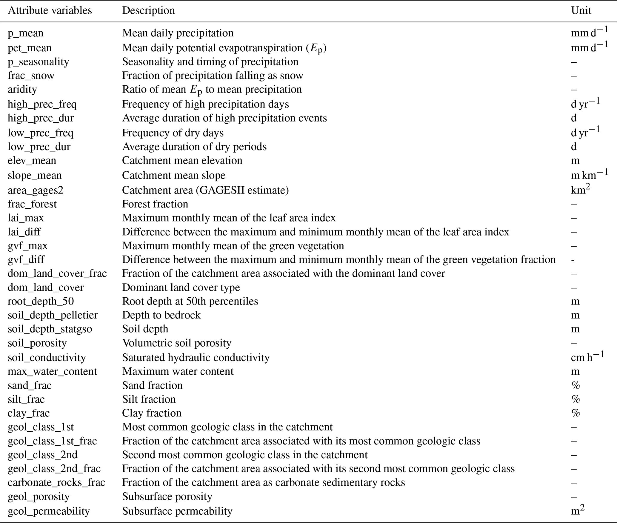
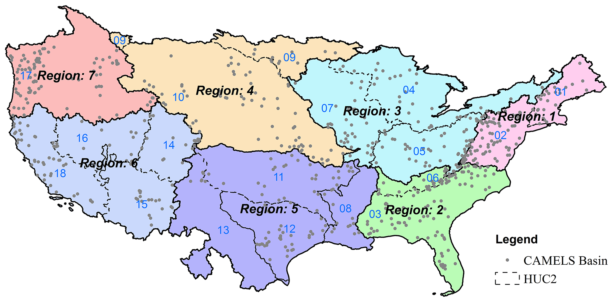
Figure B1Division of the CAMELS dataset into seven large regions for the PUR cross validation test. For every fold, the models were trained on six of the seven regions and tested on the one held out. We ran the experiments for seven rounds so that each region would be the test region once. The results for the test basins were then collected, and the test metrics were reported for this collection.
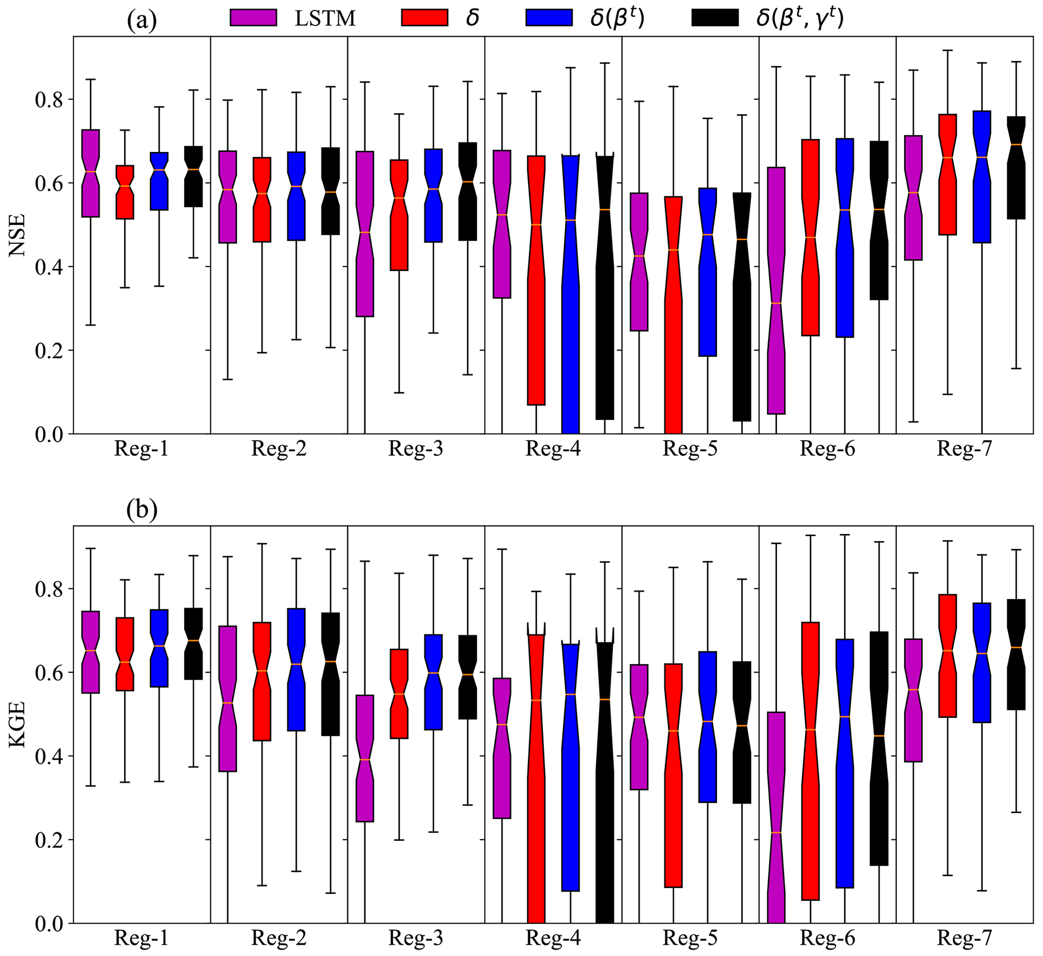
Figure B2The PUR performance comparison in different regions (shown in Fig. B1) in terms of (a) NSE and (b) KGE.
The code for the differentiable δ models is available at https://doi.org/10.5281/zenodo.7091334 (Feng et al., 2022b). The code for the LSTM streamflow model is available at https://doi.org/10.5281/zenodo.5015120 (Fang et al., 2021).
The CAMELS dataset can be accessed at https://doi.org/10.5065/D6MW2F4D (Addor et al., 2017; Newman et al., 2014). The extended Maurer forcing data for CAMELS can be downloaded at https://doi.org/10.4211/hs.17c896843cf940339c3c3496d0c1c077 (Kratzert, 2019a), and the benchmark results of traditional process-based models can be downloaded at https://doi.org/10.4211/hs.474ecc37e7db45baa425cdb4fc1b61e1 (Kratzert, 2019b). The MODIS ET product can be downloaded at https://doi.org/10.5067/MODIS/MOD16A2.006 (Running et al., 2017).
DF and CS conceived this study and designed the experiments. DF developed the differentiable models and ran the experiments. DF analyzed the results together with CS, HB, and KL. CS supervised the study. DF and CS wrote the initial draft, and all authors reviewed and edited the paper.
Kathryn Lawson and Chaopeng Shen have financial interests in HydroSapient, Inc., a company which could potentially benefit from the results of this research. This interest has been reviewed by The Pennsylvania State University in accordance with its individual conflict of interest policy for the purpose of maintaining the objectivity and the integrity of research. The peer-review process was guided by an independent editor, and the authors also have no other competing interests to declare.
Publisher’s note: Copernicus Publications remains neutral with regard to jurisdictional claims in published maps and institutional affiliations.
The differentiable hydrologic models were implemented on the PyTorch platform (Paszke et al., 2017) that supports automatic differentiation. We thank the two anonymous referees for their helpful comments to improve the quality of this paper.
Dapeng Feng has been supported by the Office of Biological and Environmental Research of the U.S. Department of Energy (contract no. DESC0016605) and U.S. National Science Foundation (NSF; grant nos. EAR-1832294 and EAR-2221880). Chaopeng Shen has been funded by the National Oceanic and Atmospheric Administration (NOAA), which was awarded to the Cooperative Institute for Research to Operations in Hydrology (CIROH) through the NOAA Cooperative Agreement with the University of Alabama (grant no. NA22NWS4320003). Computational resources have been partially provided by the NSF (grant no. OAC 1940190).
This paper was edited by Fuqiang Tian and reviewed by two anonymous referees.
Addor, N., Newman, A. J., Mizukami, N., and Clark, M. P.: Catchment attributes for large-sample studies, UCAR/NCAR[data set], https://doi.org/10.5065/D6G73C3Q, 2017.
Aghakouchak, A. and Habib, E.: Application of a Conceptual Hydrologic Model in Teaching Hydrologic Processes, Int. J. Eng. Educ., 26, 963–973, 2010.
Baker, N., Alexander, F., Bremer, T., Hagberg, A., Kevrekidis, Y., Najm, H., Parashar, M., Patra, A., Sethian, J., Wild, S., Willcox, K., and Lee, S.: Workshop report on basic research needs for scientific machine learning: Core technologies for artificial intelligence, USDOE Office of Science (SC), Washington, D.C., USA, https://doi.org/10.2172/1478744, 2019.
Baydin, A. G., Pearlmutter, B. A., Radul, A. A., and Siskind, J. M.: Automatic differentiation in machine learning: A survey, J. Mach. Learn. Res., 18, 1–43, 2018.
Beck, H. E., van Dijk, A. I. J. M., de Roo, A., Miralles, D. G., McVicar, T. R., Schellekens, J., and Bruijnzeel, L. A.: Global-scale regionalization of hydrologic model parameters, Water Resour. Res., 52, 3599–3622, https://doi.org/10.1002/2015WR018247, 2016.
Beck, H. E., Wood, E. F., McVicar, T. R., Zambrano-Bigiarini, M., Alvarez-Garreton, C., Baez-Villanueva, O. M., Sheffield, J., and Karger, D. N.: Bias correction of global high-resolution precipitation climatologies using streamflow observations from 9372 catchments, J. Climate, 33, 1299–1315, https://doi.org/10.1175/JCLI-D-19-0332.1, 2020a.
Beck, H. E., Pan, M., Lin, P., Seibert, J., Dijk, A. I. J. M. van, and Wood, E. F.: Global fully distributed parameter regionalization based on observed streamflow from 4,229 headwater catchments, J. Geophys. Res.-Atmos., 125, e2019JD031485, https://doi.org/10.1029/2019JD031485, 2020b.
Bergström, S.: Development and application of a conceptual runoff model for Scandinavian catchments, PhD Thesis, Swedish Meteorological and Hydrological Institute (SMHI), Norköping, Sweden, http://urn.kb.se/resolve?urn=urn:nbn:se:smhi:diva-5738 (last access: 8 June 2022), 1976.
Bergström, S.: The HBV model – its structure and applications, Swedish Meteorological and Hydrological Institute (SMHI), Norrköping, Sweden, https://www.smhi.se/en/publications/the-hbv-model-its-structure-and-applications-1.83591 (last access: 8 June 2022), 1992.
Beven, K.: A manifesto for the equifinality thesis, J. Hydrol., 320, 18–36, https://doi.org/10/ccx2ks, 2006.
Boretti, A. and Rosa, L.: Reassessing the projections of the World Water Development Report, npj Clean Water, 2, 1–6, https://doi.org/10.1038/s41545-019-0039-9, 2019.
Christianson, D.: Introducing the AmeriFlux FLUXNET data product, Lawrence Berkeley National Laboratory (LBNL), https://ameriflux.lbl.gov/introducing-the-ameriflux-fluxnet-data-product/ (last access: 8 June 2022), 2022.
Döll, P., Fiedler, K., and Zhang, J.: Global-scale analysis of river flow alterations due to water withdrawals and reservoirs, Hydrol. Earth Syst. Sci., 13, 2413–2432, https://doi.org/10.5194/hess-13-2413-2009, 2009.
Duethmann, D., Peters, J., Blume, T., Vorogushyn, S., and Güntner, A.: The value of satellite-derived snow cover images for calibrating a hydrological model in snow-dominated catchments in Central Asia, Water Resour. Res., 50, 2002–2021, https://doi.org/10.1002/2013WR014382, 2014.
Eicker, A., Schumacher, M., Kusche, J., Döll, P., and Schmied, H. M.: Calibration/data assimilation approach for integrating GRACE data into the WaterGAP Global Hydrology Model (WGHM) using an ensemble Kalman filter: First results, Surv. Geophys., 35, 1285–1309, https://doi.org/10.1007/s10712-014-9309-8, 2014.
European Space Agency (ESA): About SMOS – Soil Moisture and Ocean Salinity mission, https://earth.esa.int/eogateway/missions/smos, last access: 8 June 2022.
Fang, K., Shen, C., Kifer, D., and Yang, X.: Prolongation of SMAP to spatiotemporally seamless coverage of continental U.S. using a deep learning neural network, Geophys. Res. Lett., 44, 11030–11039, https://doi.org/10.1002/2017gl075619, 2017.
Fang, K., Pan, M., and Shen, C.: The value of SMAP for long-term soil moisture estimation with the help of deep learning, IEEE T. Geosci. Remote, 57, 2221–2233, https://doi.org/10/gghp3v, 2019.
Fang, K., Shen, C., and Feng, D.: mhpi/hydroDL: MHPI-hydroDL (v2.0), Zenodo [code], https://doi.org/10.5281/zenodo.5015120, 2021.
Fang, K., Kifer, D., Lawson, K., Feng, D., and Shen, C.: The data synergy effects of time-series deep learning models in hydrology, Water Resour. Res., 58, e2021WR029583, https://doi.org/10.1029/2021WR029583, 2022.
Feng, D., Fang, K., and Shen, C.: Enhancing streamflow forecast and extracting insights using long-short term memory networks with data integration at continental scales, Water Resour. Res., 56, e2019WR026793, https://doi.org/10.1029/2019WR026793, 2020.
Feng, D., Lawson, K., and Shen, C.: Mitigating prediction error of deep learning streamflow models in large data-sparse regions with ensemble modeling and soft data, Geophys. Res. Lett., 48, e2021GL092999, https://doi.org/10.1029/2021GL092999, 2021.
Feng, D., Liu, J., Lawson, K., and Shen, C.: Differentiable, learnable, regionalized process-based models with multiphysical outputs can approach state-of-the-art hydrologic prediction accuracy, Water Resour. Res., 58, e2022WR032404, https://doi.org/10.1029/2022WR032404, 2022a.
Feng, D., Shen, C., Liu, J., Lawson, K., and Beck, H.: Differentiable hydrologic models: dPL + evolved HBV, Zenodo [code], https://doi.org/10.5281/zenodo.7091334, 2022b.
Frame, J. M., Kratzert, F., Raney II, A., Rahman, M., Salas, F. R., and Nearing, G. S.: Post-Processing the National Water Model with Long Short-Term Memory Networks for Streamflow Predictions and Model Diagnostics, J. Am. Water Resour. As., 57, 885–905, https://doi.org/10.1111/1752-1688.12964, 2021.
Frame, J. M., Kratzert, F., Gupta, H. V., Ullrich, P., and Nearing, G. S.: On strictly enforced mass conservation constraints for modelling the Rainfall-Runoff process, Hydrol. Process., 37, e14847, https://doi.org/10.1002/hyp.14847, 2023.
Gupta, H. V., Kling, H., Yilmaz, K. K., and Martinez, G. F.: Decomposition of the mean squared error and NSE performance criteria: Implications for improving hydrological modelling, J. Hydrol., 377, 80–91, https://doi.org/10.1016/j.jhydrol.2009.08.003, 2009.
Hannah, D. M., Demuth, S., van Lanen, H. A. J., Looser, U., Prudhomme, C., Rees, G., Stahl, K., and Tallaksen, L. M.: Large-scale river flow archives: importance, current status and future needs, Hydrol. Process., 25, 1191–1200, https://doi.org/10.1002/hyp.7794, 2011.
Hattermann, F. F., Krysanova, V., Gosling, S. N., Dankers, R., Daggupati, P., Donnelly, C., Flörke, M., Huang, S., Motovilov, Y., Buda, S., Yang, T., Müller, C., Leng, G., Tang, Q., Portmann, F. T., Hagemann, S., Gerten, D., Wada, Y., Masaki, Y., Alemayehu, T., Satoh, Y., and Samaniego, L.: Cross-scale intercomparison of climate change impacts simulated by regional and global hydrological models in eleven large river basins, Climatic Change, 141, 561–576, https://doi.org/10.1007/s10584-016-1829-4, 2017.
Hrachowitz, M., Savenije, H. H. G., Blöschl, G., McDonnell, J. J., Sivapalan, M., Pomeroy, J. W., Arheimer, B., Blume, T., Clark, M. P., Ehret, U., Fenicia, F., Freer, J. E., Gelfan, A., Gupta, H. V., Hughes, D. A., Hut, R. W., Montanari, A., Pande, S., Tetzlaff, D., Troch, P. A., Uhlenbrook, S., Wagener, T., Winsemius, H. C., Woods, R. A., Zehe, E., and Cudennec, C.: A decade of Predictions in Ungauged Basins (PUB) – a review, Hydrolog. Sci. J., 58, 1198–1255, https://doi.org/10/gfsq5q, 2013.
Innes, M., Edelman, A., Fischer, K., Rackauckas, C., Saba, E., Shah, V. B., and Tebbutt, W.: A Differentiable Programming System to Bridge Machine Learning and Scientific Computing, arXiv [preprint], https://doi.org/10.48550/arXiv.1907.07587, 18 July 2019.
Jiang, S., Zheng, Y., and Solomatine, D.: Improving AI system awareness of geoscience knowledge: Symbiotic integration of physical approaches and deep learning, Geophys. Res. Lett., 47, e2020GL088229, https://doi.org/10.1029/2020GL088229, 2020.
Kim, Y. W., Kim, T., Shin, J., Go, B., Lee, M., Lee, J., Koo, J., Cho, K. H., and Cha, Y.: Forecasting abrupt depletion of dissolved oxygen in urban streams using discontinuously measured hourly time-series data, Water Resour. Res., 57, e2020WR029188, https://doi.org/10.1029/2020WR029188, 2021.
Kratzert, F.: CAMELS Extended Maurer Forcing Data, HydroShare [data set], https://doi.org/10.4211/hs.17c896843cf940339c3c3496d0c1c077, 2019a.
Kratzert, F.: CAMELS benchmark models, HydroShare [data set], https://doi.org/10.4211/hs.474ecc37e7db45baa425cdb4fc1b61e1, 2019b.
Kratzert, F., Klotz, D., Herrnegger, M., Sampson, A. K., Hochreiter, S., and Nearing, G. S.: Toward improved predictions in ungauged basins: Exploiting the power of machine learning, Water Resour. Res., 55, 11344–11354, https://doi.org/10/gg4ck8, 2019a.
Kratzert, F., Klotz, D., Shalev, G., Klambauer, G., Hochreiter, S., and Nearing, G.: Towards learning universal, regional, and local hydrological behaviors via machine learning applied to large-sample datasets, Hydrol. Earth Syst. Sci., 23, 5089–5110, https://doi.org/10.5194/hess-23-5089-2019, 2019b.
Kratzert, F., Klotz, D., Hochreiter, S., and Nearing, G. S.: A note on leveraging synergy in multiple meteorological data sets with deep learning for rainfall–runoff modeling, Hydrol. Earth Syst. Sci., 25, 2685–2703, https://doi.org/10.5194/hess-25-2685-2021, 2021.
Landerer, F. W., Flechtner, F. M., Save, H., Webb, F. H., Bandikova, T., Bertiger, W. I., Bettadpur, S. V., Byun, S. H., Dahle, C., Dobslaw, H., Fahnestock, E., Harvey, N., Kang, Z., Kruizinga, G. L. H., Loomis, B. D., McCullough, C., Murböck, M., Nagel, P., Paik, M., Pie, N., Poole, S., Strekalov, D., Tamisiea, M. E., Wang, F., Watkins, M. M., Wen, H.-Y., Wiese, D. N., and Yuan, D.-N.: Extending the global mass change data record: GRACE follow-on instrument and science data performance, Geophys. Res. Lett., 47, e2020GL088306, https://doi.org/10.1029/2020GL088306, 2020.
Le, M.-H., Kim, H., Adam, S., Do, H. X., Beling, P., and Lakshmi, V.: Streamflow Estimation in Ungauged Regions using Machine Learning: Quantifying Uncertainties in Geographic Extrapolation, Hydrol. Earth Syst. Sci. Discuss. [preprint], https://doi.org/10.5194/hess-2022-320, in review, 2022.
Liu, J., Rahmani, F., Lawson, K., and Shen, C.: A multiscale deep learning model for soil moisture integrating satellite and in situ data, Geophys. Res. Lett., 49, e2021GL096847, https://doi.org/10.1029/2021GL096847, 2022.
Ma, K., Feng, D., Lawson, K., Tsai, W.-P., Liang, C., Huang, X., Sharma, A., and Shen, C.: Transferring hydrologic data across continents – Leveraging data-rich regions to improve hydrologic prediction in data-sparse regions, Water Resour. Res., 57, e2020WR028600, https://doi.org/10.1029/2020wr028600, 2021.
Maurer, E. P., Wood, A. W., Adam, J. C., Lettenmaier, D. P., and Nijssen, B.: A long-term hydrologically based dataset of land surface fluxes and states for the conterminous United States, J. Climate, 15, 3237–3251, https://doi.org/10/dk5v56, 2002.
Mu, Q., Zhao, M., and Running, S. W.: Improvements to a MODIS global terrestrial evapotranspiration algorithm, Remote Sens. Environ., 115, 1781–1800, https://doi.org/10.1016/j.rse.2011.02.019, 2011.
Nash, J. E. and Sutcliffe, J. V.: River flow forecasting through conceptual models part I – A discussion of principles, J. Hydrol., 10, 282–290, https://doi.org/10/fbg9tm, 1970.
Newman, A. J., Sampson, K., Clark, M. P., Bock, A., Viger, R. J., and Blodgett, D.: A large-sample watershed-scale hydrometeorological dataset for the contiguous USA, UCAR/NCAR [data set], https://doi.org/10.5065/D6MW2F4D, 2014.
Newman, A. J., Mizukami, N., Clark, M. P., Wood, A. W., Nijssen, B., Nearing, G., Newman, A. J., Mizukami, N., Clark, M. P., Wood, A. W., Nijssen, B., and Nearing, G.: Benchmarking of a Physically Based Hydrologic Model, J. Hydrometeorol., 18, 2215–2225, https://doi.org/10/gbwr9s, 2017.
National Snow and Ice Data Center (NSIDC): SMAP Overview – Soil Moisture Active Passive, https://nsidc.org/data/smap, last access: 8 June 2022.
O, S. and Orth, R.: Global soil moisture data derived through machine learning trained with in-situ measurements, Sci. Data, 8, 170, https://doi.org/10.1038/s41597-021-00964-1, 2021.
Paszke, A., Gross, S., Chintala, S., Chanan, G., Yang, E., DeVito, Z., Lin, Z., Desmaison, A., Antiga, L., and Lerer, A.: Automatic differentiation in PyTorch, in: 31st Conference on Neural Information Processing Systems (NIPS 2017), Long Beach, CA, USA, 9 December 2017, https://openreview.net/forum?id=BJJsrmfCZ (last access: 29 June 2023), 2017.
Qiu, R., Wang, Y., Rhoads, B., Wang, D., Qiu, W., Tao, Y., and Wu, J.: River water temperature forecasting using a deep learning method, J. Hydrol., 595, 126016, https://doi.org/10.1016/j.jhydrol.2021.126016, 2021.
Rahmani, F., Shen, C., Oliver, S., Lawson, K., and Appling, A.: Deep learning approaches for improving prediction of daily stream temperature in data-scarce, unmonitored, and dammed basins, Hydrol. Process., 35, e14400, https://doi.org/10.1002/hyp.14400, 2021a.
Rahmani, F., Lawson, K., Ouyang, W., Appling, A., Oliver, S., and Shen, C.: Exploring the exceptional performance of a deep learning stream temperature model and the value of streamflow data, Environ. Res. Lett., 16, 024025 https://doi.org/10.1088/1748-9326/abd501, 2021b.
Rakovec, O., Mizukami, N., Kumar, R., Newman, A. J., Thober, S., Wood, A. W., Clark, M. P., and Samaniego, L.: Diagnostic evaluation of large-domain hydrologic models calibrated across the contiguous United States, J. Geophys. Res.-Atmos., 124, 13991–14007, https://doi.org/10.1029/2019JD030767, 2019.
Ray, K., Pandey, P., Pandey, C., Dimri, A. P., and Kishore, K.: On the recent floods in India, Curr. Sci., 117, 204, https://doi.org/10.18520/cs/v117/i2/204-218, 2019.
Running, S., Mu, Q., and Zhao, M.: MOD16A2 MODIS/Terra Net Evapotranspiration 8-Day L4 Global 500 m SIN Grid V006, NASA EOSDIS Land Processes DAAC [data set], https://doi.org/10.5067/MODIS/MOD16A2.006, 2017.
Samaniego, L., Kumar, R., and Attinger, S.: Multiscale parameter regionalization of a grid-based hydrologic model at the mesoscale, Water Resour. Res., 46, W05523, https://doi.org/10.1029/2008WR007327, 2010.
Seibert, J. and Vis, M. J. P.: Teaching hydrological modeling with a user-friendly catchment-runoff-model software package, Hydrol. Earth Syst. Sci., 16, 3315–3325, https://doi.org/10.5194/hess-16-3315-2012, 2012.
Sen, P. K.: Estimates of the regression coefficient based on Kendall's tau, J. Am. Stat. Assoc., 63, 1379–1389, https://doi.org/10.2307/2285891, 1968.
Shen, C.: A transdisciplinary review of deep learning research and its relevance for water resources scientists, Water Resour. Res., 54, 8558–8593, https://doi.org/10.1029/2018wr022643, 2018.
Shen, C. and Lawson, K.: Applications of Deep Learning in Hydrology, in: Deep Learning for the Earth Sciences, John Wiley & Sons, Ltd, 283–297, https://doi.org/10.1002/9781119646181.ch19, 2021.
Shen, C., Laloy, E., Elshorbagy, A., Albert, A., Bales, J., Chang, F.-J., Ganguly, S., Hsu, K.-L., Kifer, D., Fang, Z., Fang, K., Li, D., Li, X., and Tsai, W.-P.: HESS Opinions: Incubating deep-learning-powered hydrologic science advances as a community, Hydrol. Earth Syst. Sci., 22, 5639–5656, https://doi.org/10.5194/hess-22-5639-2018, 2018.
Sivapalan, M.: Prediction in ungauged basins: a grand challenge for theoretical hydrology, Hydrol. Process., 17, 3163–3170, https://doi.org/10/cdc664, 2003.
Suen, J.-P. and Eheart, J. W.: Reservoir management to balance ecosystem and human needs: Incorporating the paradigm of the ecological flow regime, Water Resour. Res., 42, https://doi.org/10.1029/2005WR004314, 2006.
Thornton, M. M., Shrestha, R., Wei, Y., Thornton, P. E., Kao, S.-C., and Wilson, B. E.: Daymet: Daily Surface Weather Data on a 1-km Grid for North America, Version 4, ORNL DAAC, https://doi.org/10.3334/ORNLDAAC/1840, 2020.
Tsai, W.-P., Feng, D., Pan, M., Beck, H., Lawson, K., Yang, Y., Liu, J., and Shen, C.: From calibration to parameter learning: Harnessing the scaling effects of big data in geoscientific modeling, Nat. Commun., 12, 5988, https://doi.org/10.1038/s41467-021-26107-z, 2021.
Velpuri, N. M., Senay, G. B., Singh, R. K., Bohms, S., and Verdin, J. P.: A comprehensive evaluation of two MODIS evapotranspiration products over the conterminous United States: Using point and gridded FLUXNET and water balance ET, Remote Sens. Environ., 139, 35–49, https://doi.org/10.1016/j.rse.2013.07.013, 2013.
Wanders, N., Bierkens, M. F. P., de Jong, S. M., de Roo, A., and Karssenberg, D.: The benefits of using remotely sensed soil moisture in parameter identification of large-scale hydrological models, Water Resour. Res., 50, 6874–6891, https://doi.org/10/f6j4b2, 2014.
Yilmaz, K. K., Gupta, H. V., and Wagener, T.: A process-based diagnostic approach to model evaluation: Application to the NWS distributed hydrologic model, Water Resour. Res., 44, W09417, https://doi.org/10.1029/2007WR006716, 2008.
Zaherpour, J., Gosling, S. N., Mount, N., Schmied, H. M., Veldkamp, T. I. E., Dankers, R., Eisner, S., Gerten, D., Gudmundsson, L., Haddeland, I., Hanasaki, N., Kim, H., Leng, G., Liu, J., Masaki, Y., Oki, T., Pokhrel, Y., Satoh, Y., Schewe, J., and Wada, Y.: Worldwide evaluation of mean and extreme runoff from six global-scale hydrological models that account for human impacts, Environ. Res. Lett., 13, 065015, https://doi.org/10.1088/1748-9326/aac547, 2018.
Zhi, W., Feng, D., Tsai, W.-P., Sterle, G., Harpold, A., Shen, C., and Li, L.: From hydrometeorology to river water quality: Can a deep learning model predict dissolved oxygen at the continental scale?, Environ. Sci. Technol., 55, 2357–2368, https://doi.org/10.1021/acs.est.0c06783, 2021.