Estimating spatiotemporally continuous snow water equivalent from intermittent satellite observations: an evaluation using synthetic data

Accurate estimates of snow water equivalent (SWE) based on remote sensing have been elusive, particularly in mountain areas. However, there now appears to be some potential for direct satellite-based SWE observations along ground tracks that only cover a portion of a spatial domain (e.g., watershed). Fortunately, spatiotemporally continuous meteorological and surface variables could be leveraged to infer SWE in the gaps between satellite ground tracks. Here, we evaluate statistical and machine learning (ML) approaches to performing track-to-area (TTA) transformations of SWE observations in California's upper Tuolumne River watershed using synthetic data. The synthetic SWE measurements are designed to mimic a potential future P-band Signals of Opportunity (P-SoOP) satellite mission with a (along-track) spatial resolution of about 500 m. We construct relationships between multiple meteorological and surface variables and synthetic SWE observations along observation tracks, and we then extend these relationships to unobserved areas between ground tracks to estimate SWE over the entire watershed. Domain-wide, SWE inferred on 1 April using two synthetic satellite tracks (∼4.5 % basin coverage) led to percent errors of basin-averaged SWE (PEBAS) of 24.5 %, 4.5 % and 6.3 % in an extremely dry water year (WY2015), a normal water year (WY2008) and an extraordinarily wet water year (WY2017), respectively. Assuming a 10 d overpass interval, percent errors of basin-averaged SWE during both snow accumulation and snowmelt seasons were mostly less than 10 %. We employ a feature sensitivity analysis to overcome the black-box nature of ML methods and increase the explainability of the ML results. Our feature sensitivity analysis shows that precipitation is the dominant variable controlling the TTA SWE estimation, followed by net long-wave radiation (NetLong). We find that a modest increase in the accuracy of SWE estimation occurs when more than two ground tracks are leveraged. The accuracy of 1 April SWE estimation is only modestly improved for track repeats more often than about 15 d.

1 Introduction

Snow is a key component of the water cycle and a critical water resource for human and natural systems. Seasonal snowpack serves as a natural “water tower” that stores water in winter and releases it during spring and early summer. It also shifts the time of peak runoff to be more aligned with the peak water demands from agricultural and municipal water users. It therefore mitigates water shortages in summer and fall (Li et al., 2017a). Snow-dominated watersheds account for over half of the Northern Hemisphere's land area, and seasonal snowpacks (and glaciers to a much lesser extent) provide water for over one-sixth of the world's population (Barnett et al., 2005). Also, snow plays a crucial role in modulating the ecological functioning of terrestrial and aquatic ecosystems (Trujillo et al., 2012).

Snow water equivalent (SWE) is a measure of the amount of water stored in a snowpack; it is the depth of water that would result if the snowpack was melted. However, while in situ measurements of SWE have long been made at snow courses and more recently at automated snow pillows (which weigh snow accumulated on a measurement platform), these point-scale SWE measurements poorly characterize the spatial variability of SWE because of the relatively small number of observations and under-sampling in high-elevation areas where large amounts of snow accumulate (Dozier, 2011). In situ observations are further complicated by the complex snow accumulation and ablation processes (Dong, 2018). In mountainous areas, SWE has high spatial variability caused by complex physiographic and atmospheric conditions (Molotch and Bales, 2005, 2006), making SWE measurements even more challenging. Lettenmaier et al. (2015) state that spatial SWE data acquisition from satellite sensors has been elusive, especially in mountainous areas, and “deserves new strategic thinking from the hydrologic community”.

Remote sensing is attractive for snow measurements over large areas because it avoids the need to access remote areas and complex terrain (Nolin, 2010; Guan et al., 2013; Schneider and Molotch, 2016). Remote sensing also has the potential to provide spatial rather than point observations of SWE. Over the last 40 years, many studies have examined the application of satellite-based passive microwave (PM) sensors for SWE retrieval. The interest in PM-based retrievals has been motivated by (1) the many PM sensors that have been put into service for other purposes, such as the SSM/I (Special Sensor Microwave/Imager) on the DMSP (Defense Meteorological Satellite Program) satellites, and (2) PM has the capability to provide global SWE observations that are not affected by cloud cover and darkness (except when precipitating events are occurring; Foster et al., 2005). However, a number of limitations of PM-based SWE observations such as coarse spatial resolution (tens of kilometers), signal saturation for deep snow, relatively large errors in forested and topographically complex areas (Li et al., 2017b), and loss of signal during snowmelt periods when the snowpack is wet (Walker and Goodison, 1993) have severely restricted its use, especially in mountainous areas.

For these reasons, over the last few years, there has been a shift in interest within the mountain snow community to new technologies that have the potential to obtain snow measurements with higher accuracy and spatial resolution. For instance, retrieval algorithms have been developed for obtaining regional- or global-scale snow depth maps with sub-kilometer spatial resolutions (e.g., Sentinel-1 snow depth retrieval described in Lievens et al., 2022 and stereo satellite imagery described in Deschamps-Berger et al., 2020). Another avenue that has been explored for estimating SWE (rather than snow depth) directly is P-band Signals of Opportunity (P-SoOp) which has the potential to provide estimates at sub-km spatial scales. This is an emerging technology that has the capability of penetrating through dense vegetation and into the root zone (because of the long wavelength of P-band), with a reflection coefficient phase that is able to simultaneously measure SWE (of dry snow; depth of wet snow is retrievable) and root zone soil moisture (see Garrison et al., 2019 and Yueh et al., 2021 for details).

Although P-SoOP has potential advantages for SWE retrieval, due to orbital constraints, all methods noted above provide track (or narrow swath) observations rather than continuous SWE maps. However, snow distribution and snowmelt runoff generation are spatiotemporally continuous processes. Hence, developing “track-to-area” (TTA) transformation would be a key step in providing space–time continuous SWE that would significantly increase the utility and value of the track observations.

The TTA could be achieved by leveraging snow-pattern repeatability and data-assimilation techniques. For instance, based on snow-pattern repeatability, Pflug and Lundquist (2020) inferred the spatial distribution of snow depth on 7 April 2014, in California's Tuolumne watershed using snow depth observations subsampled across only a portion of the study domain (<4 %) and observed snow patterns from a different water year (WY). Their results for inferred distributed snow depth had a mean absolute error of less than about 10 %. Other studies have estimated SWE maps from track information using data assimilation. For instance, Magnusson et al. (2014) assimilated point SWE observations into a SWE modeling framework, with results that suggested an ability to transfer information from point snow observations to the distributed snow estimation. Also, Schneider and Molotch (2016) performed a real-time estimation of the spatial distribution of SWE using the regression of in situ point SWE observations combined with topographic information and historical SWE patterns.

The P-SoOP has the potential to be deployed in space and to provide direct SWE and root zone soil moisture measurements during snow accumulation periods, including near the time of peak SWE that is the most significant time for water management (Shah et al., 2018). For example, NASA's proposed SNoOPI satellite (SigNals of Opportunity: P-band Investigation) is in the planning stage (https://esto.nasa.gov/invest/snoopi/, last access: 23 December 2022) and Yueh et al. (2021) describe a satellite synthetic aperture radar concept based on P-SoOp. However, none of these P-SoOP projects are yet operational, and the issue of TTA transition that we address here will become critical as they are further developed. Furthermore, our investigation is not limited to P-SoOP but is applicable to any intermittent track-based satellite observations. Although potential methods for TTA include interpolation, statistical models, data assimilation, and machine learning (ML), here we focus on ML.

Our analysis is based on the Western US Snow Reanalysis data (WUS-SR; Fang et al. 2022, hereafter F2022) as “truth” from which we synthesize P-band SWE observations along tracks, and in turn explore TTA transformation strategies. The TTA transformation of along-track SWE observations are achieved using statistical and ML approaches. Specifically, we address the following four questions: (1) How does the spatially distributed SWE inferred from TTA on 1 April compare with the synthetic truth, and how do their differences vary in dry, normal and wet years? (2) What are the dominant variables for SWE estimation of 1 April in statistical and ML TTA methods, and which method has the highest accuracy? (3) How does the accuracy of the domain-wide SWE estimates from TTA approaches evolve within a season at different temporal observation resolutions? (4) How does the performance of TTA change as a function of the spatial sampling density (number of hypothetical ground tracks), and what is the preferred number of tracks? Our study is intended to provide a pathway forward in support of future snow satellite design and SWE estimation over snow-covered areas globally.

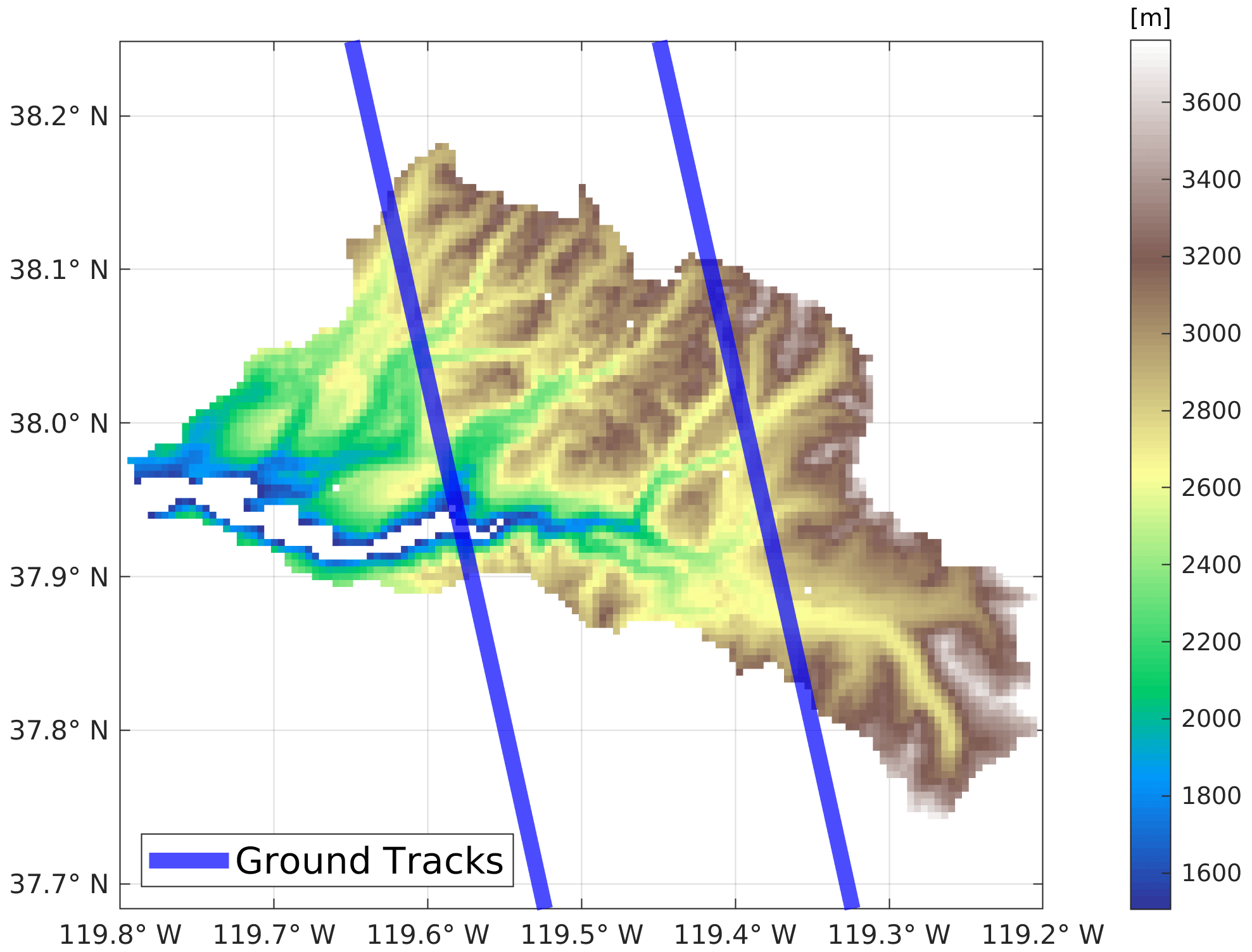
Figure 1 Elevation of the upper Tuolumne watershed (above Hetch Hetchy Reservoir). Blue lines are the synthetic ground tracks passing through the study domain. The hypothetical tracks are about 1 km wide and the distance between the two tracks is approximately 21 km.

2 Study area and data

2.1 Study area

Our study area is the upper Tuolumne watershed (above Hetch Hetchy Reservoir) in the Sierra Nevada of California. This Tuolumne basin has a drainage area of approximately 1650 km² that is characterized by complex high-elevation topography (Figs. 1 and S1 in the Supplement). Elevations in the watershed range from about 700 to 3900 m, with most of the basin area located above 2500 m (Fig. 1). Slopes are distributed between 0 and greater than 50^∘ and the terrain surface mostly has NW and SE facing aspects. Fractional vegetation cover ranges from 0 % (in high-elevation areas) to up to 60 % in low-elevation areas. The runoff in the upper Tuolumne watershed is dominated by snow with a substantial high-elevation contribution (30 % of its runoff originates from elevations of 3000 m and above). In this respect, it is typical of many watersheds that head in the Sierra Nevada and supply much of California's water.

2.2 Data

We leveraged the F2022 snow reanalysis data as the basis for our synthesis of satellite observations along ground tracks. The F2022 dataset is available for entire water years (October–September), including the wet snow period after peak SWE. The period of record is WY1985 through 2019. The spatial resolution of F2022 is 480 m, so the data size of the synthetic snow observations is 480 m, and all the synthetic tracks are 960 m wide (two 480 m pixels in width). This dataset was generated (by F2022) based on a Bayesian snow reanalysis framework with ensemble prior SWE estimates updated by assimilating fractional snow-covered area (fSCA) observations from the Landsat satellite platforms using a Particle Batch Smoother approach (Margulis et al., 2015). Prior SWE estimates (required by the data-assimilation approach) were derived from the land surface model SSiB-SAST (Sun and Xue, 2001; Xue et al., 2003) with the Liston (2004) snow depletion curve. The F2022 shows that the reanalysis SWE estimates match in situ observations of peak SWE well across the Sierra Nevada, with a mean difference of −13 cm and correlation coefficient 0.86 taken over 1432 site years of observations.

We sub-sampled the snow reanalysis data along the postulated ground tracks to synthesize the SWE observations that P-band sensors would produce (see Sect. 3.1 for details). We also used F2022 as the SWE “truth” to evaluate our TTA SWE data-transformation accuracy.

We used meteorological variables and static parameters including topographical characteristics and vegetation cover data as the ML training inputs (along ground tracks) and as the model inputs (full-domain). The ML training samples and domain-wide model inputs are from F2022. Meteorological forcings included precipitation (PPT), air temperature (T_a), surface air pressure (P_s), specific humidity (q), net short-wave radiation (NetShort), net long-wave radiation (NetLong), and wind speed (wind). The meteorological forcing fields were obtained from the Modern-Era Retrospective analysis for Research and Applications, version 2 (MERRA-2;. Gelaro et al., 2017) updated via the F2022 snow data assimilation. The digital elevation model (DEM) was obtained from the Shuttle Radar Topography Mission (SRTM; Farr et al., 2007), with gaps filled by the global digital elevation model (GDEM, version 2) product of the Advanced Spaceborne Thermal Emission and Reflection Radiometer (ASTER). The original spatial resolution of these two DEMs was 1 arcsec. The fractional vegetation cover data were taken from the Tree Canopy Cover (TCC) product containing the Landsat Vegetation Continuous Fields (Sexton et al., 2013). The meteorological, topographic and land cover data were resampled to the same spatial resolution of the snow reanalysis dataset (i.e., 16 arcsec). In real applications, the meteorological forcings could come from any multi-source surface and weather modeling data, e.g., weather forecast model analysis (real-time) or reanalysis (retrospective) fields.

3 Methodology

3.1 Experiment design

We addressed our four research questions (Sect. 1) via four TTA experiments. Each of the experiments used four algorithms: one statistical and three ML methods (details in Sects. 3.2 and 3.3). For all the TTA experiments, the general idea is that we use the algorithms to build a connection between the observed SWE and the meteorological and static variables along the ground tracks on the observation days; these relationships reflect the physical control of the meteorological and static variables on SWE under different terrain, landscape, meteorological and climatic conditions. We then extend these relationships to the unobserved areas and periods where and when meteorological and static variables are available to estimate SWE across the entire basin.

In the experiments, the target day can be any date (not necessarily one for which there is a satellite overpass). We used observations with close temporal proximity to train the four algorithms. For example, if we intend to fill the spatial SWE gaps on 1 April, our target day would be 1 April and we used the SWE (track) observations available within a short period before or on the target day for model training.

We first focused on estimating spatially continuous peak annual SWE in the basin because of its water resource importance (Sect. 3.2.1). We then explored the seasonal evolution of the TTA SWE estimation, where we sequentially set the target day to be all days within a water year to obtain spatially and temporally continuous SWE estimates over the entire Tuolumne basin (Sect. 3.2.2). Furthermore, we conducted two experiments to evaluate the impact of meteorological variable and SWE sample density on the accuracy of the SWE estimates (Sect. 3.2.3 and 3.2.4). The two experiments introduced in Sect. 3.2.3 and 3.2.4 aim to align with explainable artificial intelligence (AI; e.g., Chakraborty et al., 2021; Dikshit and Pradhan, 2021a, b; Kratzert et al., 2019), which facilitates the comprehension and trust of the results and outputs created by ML algorithms. A major objective of explainable AI is to overcome the black-box nature of ML systems, which is particularly important for hydrologic applications that are mostly process-oriented.

We used four metrics to quantify the performance of our TTA experiments: (1) mean absolute errors (MAE), (2) median (50th percentile) of percent absolute error at a pixel-level (PAE_50), (3) 90th percentile of percent absolute error at a pixel level (PAE_90), and (4) percent error of basin-averaged SWE (PEBAS). When calculating PAE_50 and PAE_90, we first calculated the percent absolute error of SWE estimates for each pixel within the study area, and then found the median and the 90th percentile of the pixel-level percent errors. To avoid extremely high percent errors due to zero or nearly zero SWE values, we filtered out pixels with SWE truth less than 50 mm when calculating PAE_50 and PAE_90. For annual peak SWE estimation (see Sect. 3.2.1 and 4.1 for details), we also calculated the bias ratio to quantify the degree of over- or underestimations of our TTA transformations.

3.2 Model training, estimation and output correction

3.2.1 Annual peak SWE estimation

In the annual peak SWE estimation experiment, we sought to fill spatial gaps between ground tracks on 1 April of 3 target years: WY2015, WY2008 and WY2017. The SWE on 1 April has long been used as a proxy of peak snow water resource availability and is a critical variable for seasonal streamflow forecasting. We selected WY2015, WY2008 and WY2017 as the extremely dry, normal and extremely wet years, respectively because they had the lowest (∼50.4 % of the average of the MERRA2 gridded-based precipitation between WY1985 to WY2019), normal (∼96.8 % of average), and highest (∼174.0 % of average) winter (1 November to 31 March) precipitation over the recorded period. To train the models for each of the 3 target years, we assumed that we had 7 SWE observations before and on 1 April in the target year and the 2 years ahead of that target year, and the temporal interval between observations within each of the 3 years was 5 d. For example, for the SWE TTA on 1 April WY2008, we used observations from late February to 1 April of WY2008, WY2007 and WY2006. On each observation day, we assumed that there were two ground tracks at the same locations that cover approximately 4.5 % of the study area (Fig. 1). We also selected 12 typical years from WY2000 to 2019. Among the 20 years, we defined wet years as the 4 years with the greatest winter precipitation, the dry years as the 4 years with the least winter precipitation, and normal years as the 4 years with winter precipitation closest to the median. We performed TTA transformation experiments for the selected 12 years to better understand the impacts of climate conditions on the accuracy of domain-wide SWE estimation near the time of peak SWE time.

The training target is to reproduce the synthetic SWE observations along the two ground tracks. The training input features include the 5 d averaged meteorological forcings within each 5 d observation cycle (i.e., each observation day and the 4 d ahead) and static variables, which include topographical and vegetation cover data along the two hypothetical ground tracks (Fig. 1). The training builds the connection between all available training input features and target pairs. After the connections are built along the ground tracks (i.e., models are trained), we used the domain-wide 5 d averaged meteorological forcings (i.e., from 28 March to 1 April) and static variables as the input to the trained models to estimate domain-wide SWE on 1 April in the target year.

After the estimation step, we implemented an error correction to the domain-wide SWE estimates. Specifically, we first conducted probability density function (PDF) matching between the estimated SWE on the ground tracks and the synthetic true SWE along the ground tracks and applied the derived PDF correction to the off-track pixels. These corrections aimed to leverage the observations on the synthetic ground tracks to eliminate systematic biases and large errors in domain-wide SWE estimates.

3.2.2 Seasonal basin-wide SWE estimation

We also applied the TTA transformation for each day over a full water year, assuming that the temporal interval between satellite observations was 0, 5, 10, 15, 20 or 30 d. We investigated the performance of the SWE TTA estimation in different phases of a snow season (i.e., accumulation, peak, and melting periods) and the sensitivity of the performance to the observation frequency.

The seasonal SWE TTA transformation filled both the spatial and temporal gaps of SWE observations. In the seasonal TTA estimation with a fixed observation interval, on the days with SWE observations, we only need to fill the spatial gaps, so the training and estimation processes in this case are identical with the 1 April experiment (as in Sect. 3.2.1). During the temporal gaps between SWE observations, the target days have no SWE observations to train the statistical and ML models, so we used the established model from the closest previous observation day and input the domain-wide forcings (5 d averaged before and on the target day) and static variables to the borrowed models from the closest previous observation day to obtain domain-wide SWE estimates on this non-observed day. We performed a PDF-matching correction for the domain-wide estimates based on the closest (in time) previous observations on ground tracks.

After SWE estimation was implemented for every day over a full water year, we obtained daily and spatially continuous SWE maps for the upper Tuolumne basin for full water years 2015, 2008 and 2017. We calculated the daily time series of basin-averaged SWE by averaging SWE values for all pixels in the study domain and compared the estimated daily basin-averaged SWE with that computed from the synthetic truth.

3.2.3 Sensitivity of TTA to input meteorological forcings

We performed an analysis of the TTA sensitivity to the input meteorological forcing fields on the 1 April SWE TTA transformation. In so doing, the training and estimation setups were the same as those in Sect. 3.2.1, except that we employed the following two methods to investigate the sensitivity of the basin-wide SWE estimates to the input meteorological forcings:

1. Missing feature analysis: we withheld one training meteorological variable during the training process each time and re-trained all four models with the remaining training fields. The change in the estimated basin-wide SWE compared with the original SWE estimates (i.e., the outputs from the model trained with all the forcing fields) could reflect the influence of this missing feature on domain-wide SWE estimates. We normalized the absolute change of MAE as an indicator to quantify the relative contribution and the magnitude of influences of each meteorological forcing field to SWE estimation.

2. Forcing uncertainty analysis: for each pixel, we perturbed each training meteorological field with a percentage error (−50 % to 50 % with an interval of 1 %), and each time we perturb only one field while holding the other forcing fields unchanged. A 0 % error meant that the meteorological inputs were the same as their original values (i.e., the same as what we used in the experiment described above). A β % (β is a constant here) error meant that we added β % of the difference between the maxima and minima of a specific variable within the study period (i.e., 1985 to 2019) for this pixel to the original value. Every time we added more error to a training field, we re-trained the statistical and ML models. We then used the trained model to predict the basin-wide SWE and used MAE to quantify the SWE estimate errors caused by the error perturbation. With the 100 realizations for each training field (−50 % error to 50 % error with an interval of 1 %), we explored the corresponding changes in domain-wide SWE estimates, which allowed us to determine the influence of forcing errors on SWE estimates and identify sources of model errors.

3.2.4 Sensitivity to the number of ground tracks

The investigations discussed above were all based on the two hypothetical ground tracks shown in Fig. 1. To explore the relationship between the number of ground tracks and estimation accuracy, we assumed that there were 1–6 overpasses covering from 2.42 % to 12.10 % of the study area on 1 April, so that the available observations for model training vary with the different numbers of tracks passing through the watershed. All the tracks in each scenario were distributed over the entire Tuolumne basin with equal spacing. The training and estimation processes were the same as the experiment on 1 April (details in Sect. 3.2.1).

3.3 Satellite observation gap-filling methods

We utilized and compared the four algorithms to transform the postulated track-based satellite observations into space-continuous SWE estimates, as described below.

3.3.1 Statistical method

As applied, multivariate linear regression (MVLR) defines a linear relationship between multiple independent variables (input variables) and one dependent variable (the target variable) based on pre-defined rules, e.g., the regressed results are Best Linear Unbiased Estimator (BLUE) of the dependent variable (see Sect. S1 in the Supplement for details). In our case, this refers to the input variables were the meteorological forcings and static land cover features; the target variable was SWE.

3.3.2 Machine learning algorithms

We explored three machine learning (ML) methods: random forest (RF; Breiman, 2001), support vector machines (SVM; Vapnik, 1982), and deep neural networks (DNN; Tanaka and Okutomi, 2014) on building the relationship between inputs and SWE along ground tracks. The hyperparameters of the three ML methods were optimized using 10-fold cross validation. After the selection of model hyperparameters, we train each model 10 times. During each of the 10 training cycles, we randomly reserved 15 % of the training dataset as the test the dataset that was used for evaluating the estimation results, we trained the three ML models using the remaining 85 % of the training dataset and estimated model performance using the test dataset. The 10-fold cross validation repeated this training-validating process 10 times with the training (85 %) and validation (15 %) sub-dataset randomly selected each time. After the 10 cycles, we selected the 5 model setups with the lowest MAE for the test dataset and used these 5 selected model sets with domain-wide input features to obtain 5 sets of SWE estimates over the whole watershed. Our final domain-wide SWE estimates were the average of the SWE estimates from the 5 selected models.

Random forest

We used the random forest (RF) method introduced by Breiman (2001), implemented to simulate the non-linear relationship between input features and SWE. The basic building units of RF are an ensemble of decision trees (DTs) that split a subset of features on each split (Kuter, 2021). Usually, a series of DTs is employed to achieve sufficient accuracy of final prediction by weighted averaging the prediction results of multiple selected DTs (Liu et al., 2020). The selection of DTs was carried out by voting, that is, the higher the repetition degree of the DT, the higher the contribution of this DT to the RF model.

During the training process, we optimized two hyperparameters in the RF system: (1) Ntree – the number of decision trees grown based on a bootstrap sample of observations; (2) Sleaf – minimum number of observations per tree leaf. One useful characteristic of RF is that it is a self-explainable model where the implementation and examination of the out-of-bag score is a form of model validation. To optimize the two hyperparameters, we carried out 10-fold cross validation to find the optimal hyperparameter combinations with the lowest out-of-bag errors. The change of errors with Ntree and Sleaf were shown in Figs. S2 and S3. Our analysis showed that the preferred number of decision trees was 50 and the minimum leaf size was 5.

Support vector machine

Support vector machine (SVM) method is a supervised and non-parametric ML algorithm (Vapnik, 1982). For regression-based SVM, the basic logic behind the learning task is to find a function that has the universal minimum deviation from the measured response values for the full range of observations (Vapnik, 1998).

During the training process of the SVM method, we mainly optimized two hyperparameters: (1) the kernel function, which specifies the method used to transform inputs to the required target, and (2) the kernel scale, which is a scaling parameter for the input data. Based on 10-fold cross validation, we specified the Gaussian kernel function and selected the kernel scale based on a heuristic procedure, which used the subsampling and set a random number seed before training, so estimates can vary for every running process.

Deep neural network

Artificial neural network (ANN) builds a non-linear relationship between the independent variables and the target variable by connecting neurons in one layer to the previous or next layers. In general, ANN is a multi-layer structure that includes an input layer, one hidden layer, and an output layer. The hidden layer consists of several neurons, each of which is assigned a weight. The output of each neuron is multiplied by the weight and serves as the input for a non-linear activation function (Abiodun et al., 2018). A single-layer perceptron is a neural network with only one neuron that can only understand linear relationships between the input and output data, while with horizons of the deep neural network (DNN), a multilayer perceptron (MLP), are expanded and the neural network can have multiple layers of neurons, which are better adapted to more complex patterns (Gardner and Dorling, 1998). Here, we built an MLP and tested several combinations of the number of hidden layers and the number of neurons in each hidden layer; we also constructed a seven-layer neural network (which was essentially an MLP) with 10, 9, 8, 7, 6, 5 and 4 neurons in each layer, respectively. We chose rectified linear units (ReLu) as the activation function in each hidden layer. In this network, the algorithm used to minimize the cost function is Levenberg–Marquardt, which is considered as one of the most efficient learning algorithms in terms of convergence speed (Costa et al., 2007).

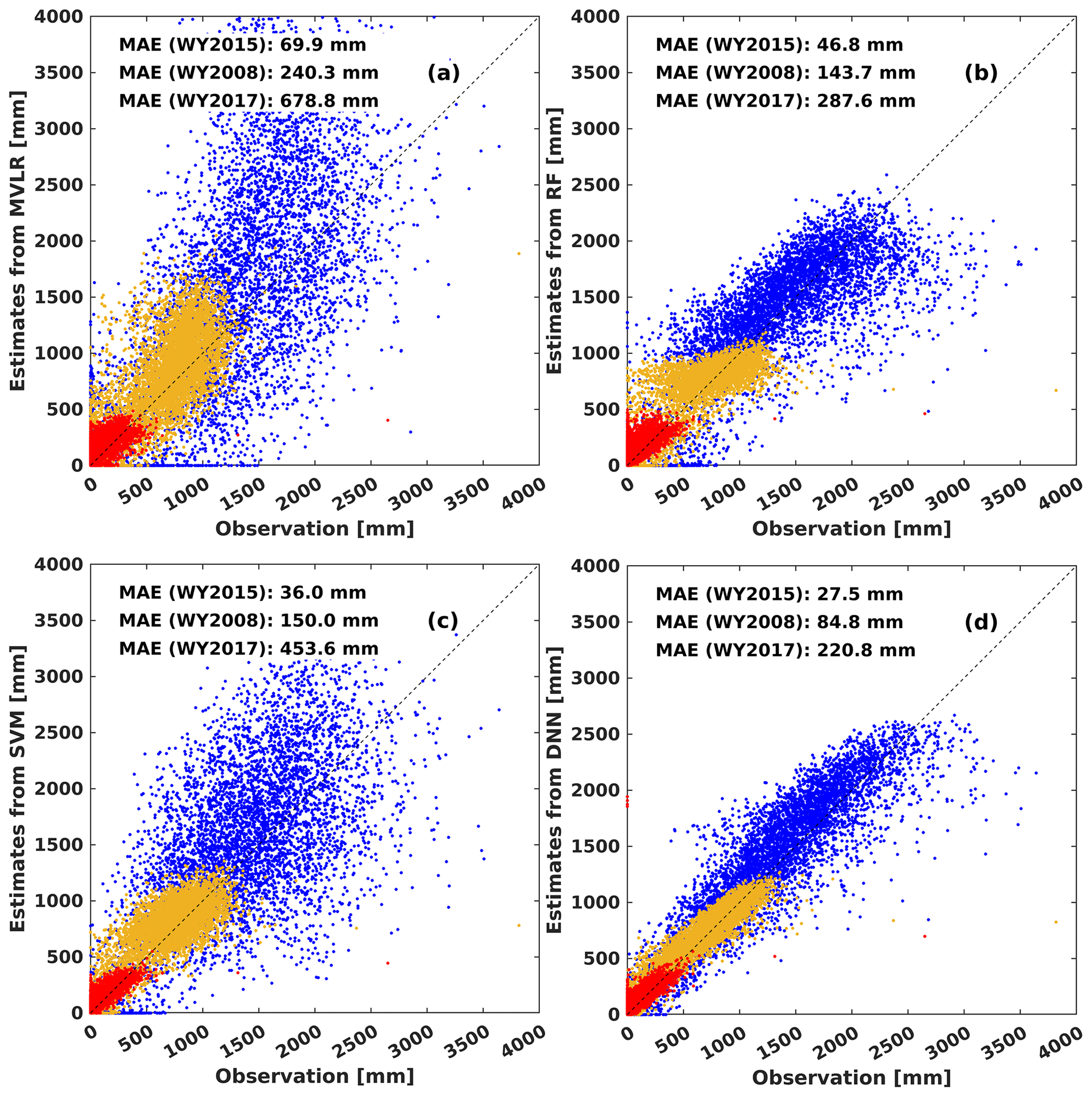
Figure 2 Pixel-level scatterplots of 1 April SWE estimated by MVLR (a), RF (b), SVM (c), and DNN (d) versus the true 1 April SWE in WY2015 (dry year; red dots), WY2008 (normal year; yellow dots), and WY2017 (wet year; blue dots).

4 Results and discussion

4.1 Basin-wide SWE estimation on 1 April

Figure 2 shows pixel-level results for all four algorithms on 1 April for WY2008, WY2015 and WY2017. The DNN generally outperforms the other three methods, which has fewer outliers with results distributed closer to the 1:1 line on the scatterplot. Statistically, domain-wide SWE estimates from DNN are also the best among the four methods, except that RF performs slightly better than DNN in terms of PEBAS in the normal and wet years (Figs. 2 and 3). The DNN-based estimates have (1) the lowest values of MAE (Fig. 2); (2) the highest accuracy from the perspective of PEBAS in the dry year (Fig. 3); and (3) at a pixel level, the lowest values of PAE_50 and PAE_90 (Fig. 3). A possible reason why DNN outperforms RF is that during the training process of RF, the discretization of continuous variables in the DT generation leads to a reduction in the number of nodes and therefore the loss of part of the information (Segal, 2004). Also, SVM has some disadvantages, such as not being suitable for large datasets and the decision model does not perform well when the dataset is noisy. The MVLR is the worst among the four algorithms, probably because MVLR is only capable of simulating linear relationships between model inputs and outputs, while the process of SWE estimation involves more complex non-linear relationships.

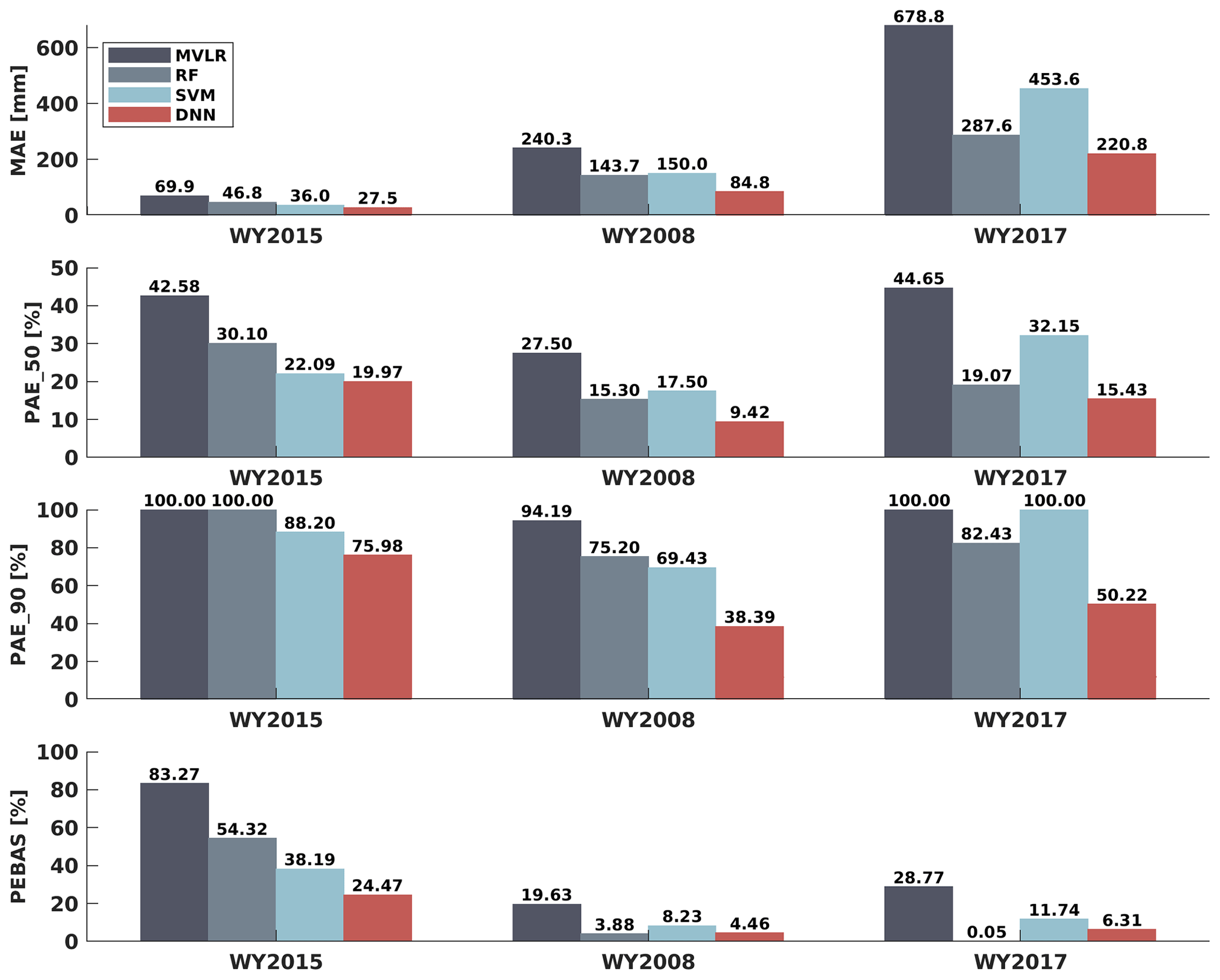
Figure 3 Mean absolute error (MAE), median of percent absolute error (PAE_50), 90th percentile percent absolute error (PAE_90) and percent error of basin-averaged SWE (PEBAS) of domain-wide SWE estimates based on MVLR, RF, SVM and DNN in WY2015 (dry year), WY2008 (normal year) and WY2017 (wet year).

Accurate SWE estimation in the extremely dry year is of key importance for water management in California. Figure 2d shows that domain-wide SWE estimates in the extremely dry year (WY2015) are nearly unbiased for MVLR and DNN, but RF and SVM tend to overestimate SWE (Fig. 2). All ML-based domain-wide SWE estimates in WY2015 have higher accuracy than the statistical method (Figs. 2 and 3). The DNN performs the best among the four algorithms in WY2015 in terms of MAE (27.5 mm), PAE_50 (20.0 %), PAE_90 (76.0 %) and PEBAS (24.5 %).

Machine learning methods are also more accurate than the statistical method in the typical (normal) year (WY2008). Compared to the three ML algorithms, the statistical method has the largest MAE, PAE_50, PAE_90 and PEBAS in WY2008 (Fig. 3). Compared to the dry year, SWE estimates are more accurate in the normal year in terms of PAE_50, PAE_90 and PEBAS for all four algorithms. Possible reasons for the better performance in the normal year relative to the dry year include the following: (1) the number of pixels with zero SWE value is much less in the normal year than in the dry year, so the useful training information for building the relationship between inputs and the target are more abundant in the normal year; (2) there are fewer pixels with small values of SWE in the normal year than in the dry year, and small SWE values tend to generate large values in percentage error calculation, so the values of metrics regarding percent errors are larger in the dry year. The reason for larger values of PAE_90 in the dry year (DNN: 76.0 %) than in the normal year (DNN: 38.4 %) is that although we omitted pixels with extremely small SWE (<50 mm), in the dry year, there are still more pixels with low SWE, which are prone to high percent errors. The TTA SWE estimation is weakest in low-SWE situations, resulting in heavy-tailed behavior in the percent SWE errors under that condition.

The ML-based estimates were also most accurate in the extremely wet year (WY2017). According to the estimation statistics, DNN is the best algorithm among the four TTA transformation methods with the lowest MAE (220.8 mm), PAE_50 (15.4 %), PAE_90 (50.2 %) and PEBAS (6.3 %). Compared to the normal and dry years, the wet year has fewer pixels with zero or nearly zero SWE values, thus the number of useful pixels for training ML algorithms is larger. Also, SWE values are larger, which tends to reduce the percent absolute errors, making PAE_50 and PAE_90 values generally smaller than those in the dry or normal years.

Overall, DNN outperforms the other three algorithms for all 3 years (Figs. 2 and 3), while the statistical method (MVLR) has larger values of MAE, PAE_50, PAE_90 and PEBAS than all the ML methods for all the 3 years. Due to the superior performance of DNN, the following results and discussion are based on DNN only; results for the other three methods are included in the supplemental material.

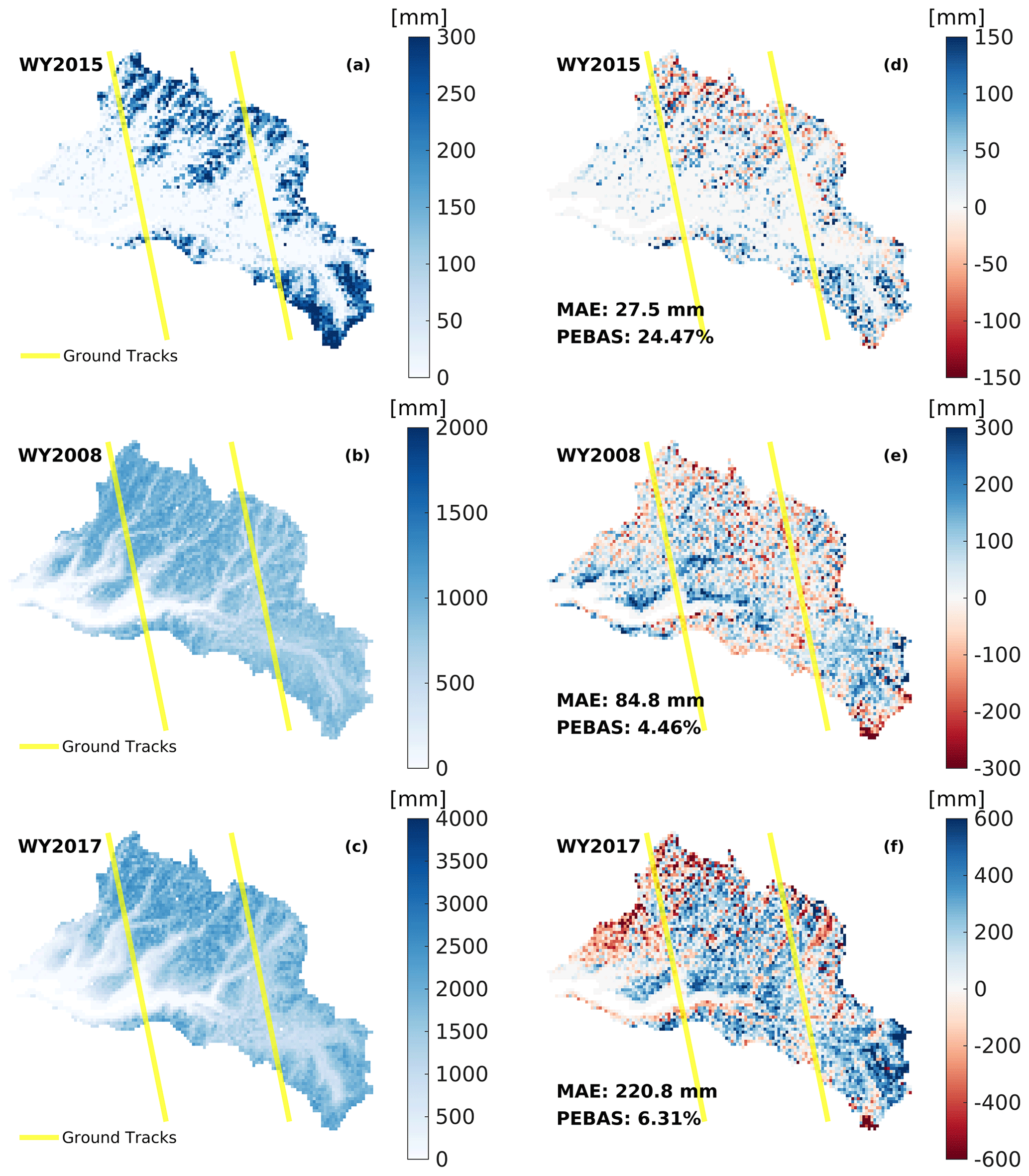
Figure 4 DNN-inferred 1 April SWE maps (a–c) and 1 April SWE errors (estimate minus truth; d–f) in WY2015, WY2008 and WY2017. Yellow lines are hypothetical ground tracks across the upper Tuolumne watershed, which are approximately 1 km wide and the distance between the two tracks is around 21 km.

The SWE on 1 April is highly correlated with cumulative winter precipitation, so SWE estimation errors tend to be small in dry years and large in wet years. Correspondingly, as shown in the spatial maps of SWE estimates and estimation errors (Fig. 4), in WY2015, for nearly all the pixels within the study area, the overall estimation errors are within the range ±200 mm (PAE_50: 20.0 % and PEBAS: 24.5 %). The error range is larger in WY2008 than in the dry year, which is about ±300 mm (PAE_50: 9.4 % and PEBAS: 4.5 %) and larger still (±500 mm) in WY2017 (PAE_50: 15.43 % and PEBAS: 6.31 %).

The spatial maps of DNN-based domain-wide SWE estimation errors (Fig. 4d–f) show that the patterns of error distribution are similar for the 3 years, that is, underestimates are more likely to appear in the low-elevation areas in the western watershed (elevation range: around 1500 to 2800 m) while overestimates appear mainly in the high-elevation areas in the northern parts of the watershed (elevation range: approximately 2800 to 3800 m), especially in the normal and wet years (i.e., WY2008 and WY2017). A possible explanation for this error pattern is that during the training process, ML models would leave out some outliers, some of which are probably the extreme values in low- or high-elevation areas, thus the estimates from the ML systems may tend to approach an average situation, that is, predict higher for low values and lower for high values. Pixels in the low-elevation areas generally have low SWE, therefore overestimates tend to occur in these regions; in contrast, underestimation tends to occur more for pixels in high-elevation areas.

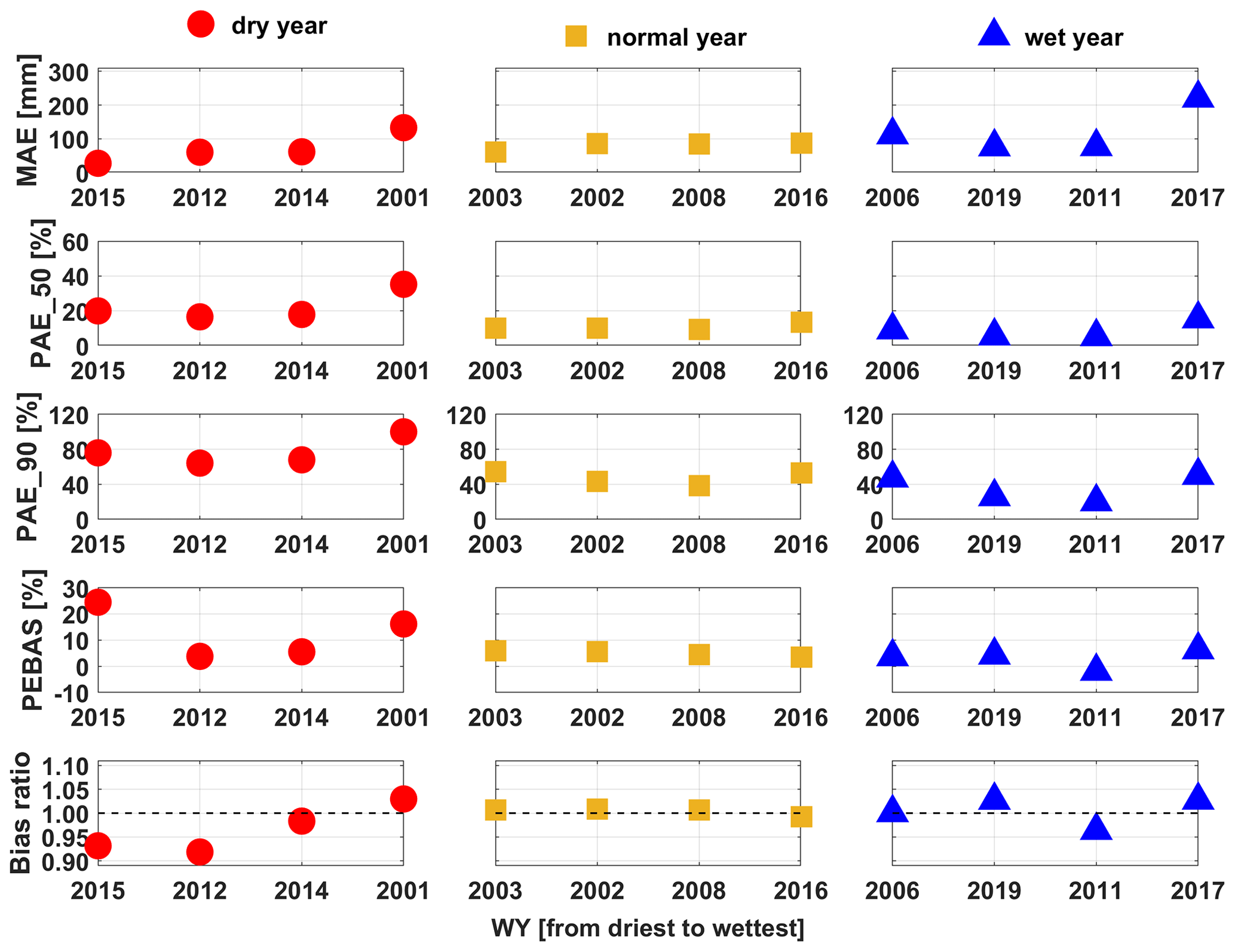
Figure 5 MAE (mm; first row), PAE_50 (%; second row), PAE_90 (%; third row), PEBAS (%; fourth row) and bias ratio (slope; fifth row) of the DNN-based estimated 1 April SWE for the 4 driest years (red dots; WY2015, 2012, 2014 and 2001), 4 normal years (yellow square points; WY2003, 2002, 2008, and 2016) and 4 wettest years (blue triangle points; WY2006, 2009, 2011, and 2017) from WY2000 to WY2019.

We also evaluate errors in domain-wide 1 April SWE for a larger number (12) of years (4 driest, 4 normal and 4 wettest years from WY2000 to WY2019) to better understand the impacts of climate conditions on the accuracy of domain-wide SWE estimation near the time of peak SWE time (Fig. 5). The metrics used to quantify the accuracy of SWE estimation include MAE, PAE_50, PAE_90, PEBAS and bias ratio (slope of the regression line (intercept was forced to be 0) between estimation and truth). Our results indicate that overall, the MAE of 1 April SWE estimates becomes larger as precipitation increases (MAE: wet years > normal years > dry years). For example, the MAE in WY2017 is twice as large as the average MAE of the other years (MAE in WY2017: 220.8 mm; average MAE of the other years: 79.3 mm). This is likely because SWE is largely determined by the amount of winter precipitation in the given year. To better compare the performance of DNN-based TTA transformation in different water years with climate conditions, we further show the PAE_50, PAE_90 and PEBAS for each of the 4 years. According to PAE_50, at a pixel level, half of the pixels have absolute percent errors smaller than 20 % (except for WY2001), even in the 4 driest years when extremely low SWE values may lead to large values of percent absolute errors for many pixels in the study area. As noted above, the PAE_90 values are relatively large in the dry years; on the other hand, the values of PAE_90 are smaller than or close to 50 % in the normal and wet years, indicating that 90 % of the pixels in the study area have relatively small SWE estimation errors. In addition, the values of PEBAS are less than 20 % for all years except for WY2015 (which has zero 1 April SWE in many locations that had not previously been snow-free during the instrumental record).

The bias ratio (quantified by the regression slope between the SWE estimate and truth with intercept forced to be 0) provides information about the degree of over- or underestimation of domain-wide SWE estimates. The bias ratio for the 12 years (Fig. 5) indicates that DNN provides an approximately unbiased estimate of domain-wide SWE across all climate conditions with slopes of the zero-intercept regressions, all within the range 0.9–1.1. In the normal years, all slope values are close to 1.0 (WY2003: 1.01; WY2002: 1.01; WY2008: 1.01; WY2016: 0.99). The SWE estimation modestly degrades under dry and wet conditions with slight underestimation of SWE (with a bias ratio around 0.93) in the 2 driest years (Fig. 5).

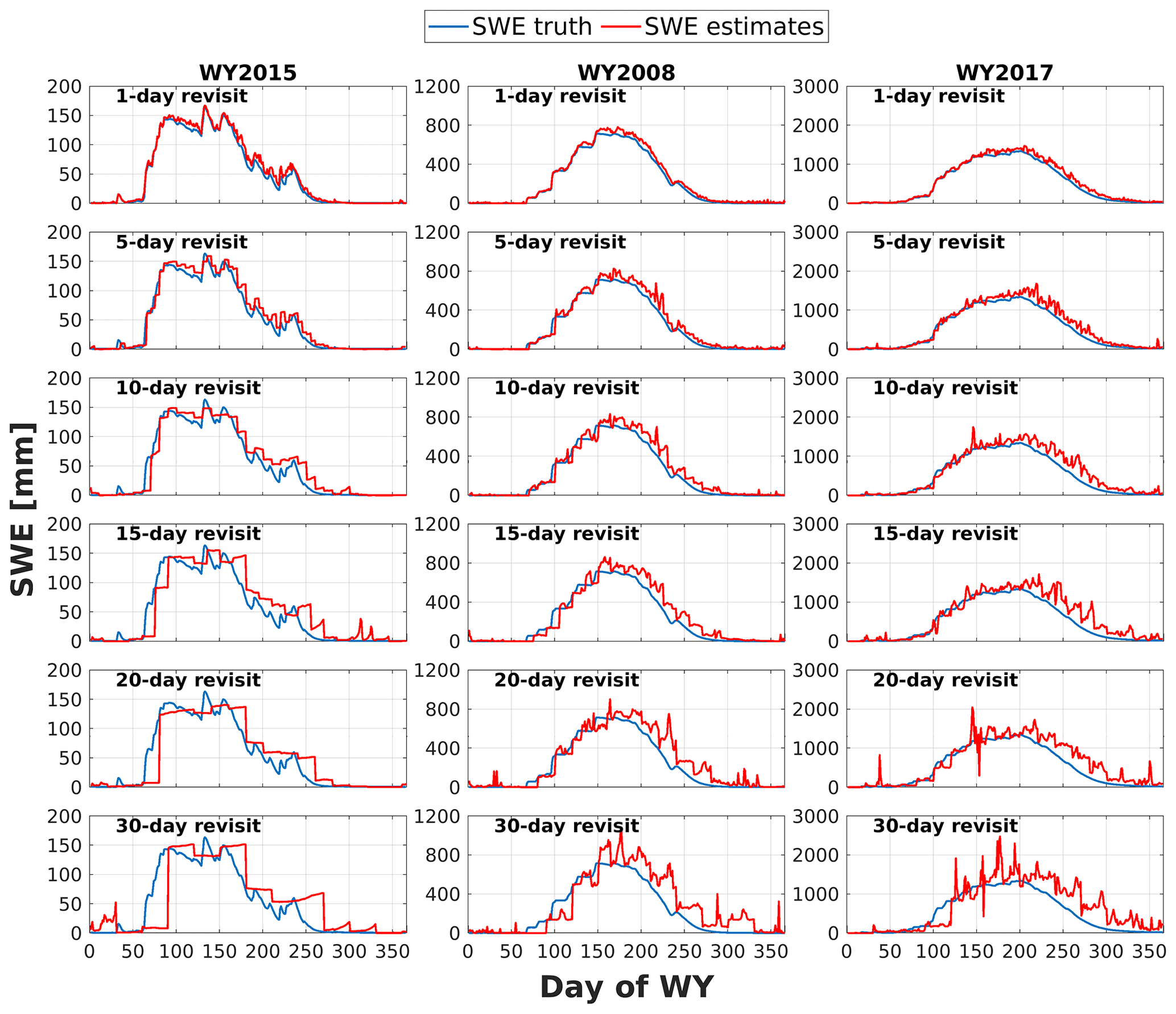
Figure 6 Daily time series of basin-averaged SWE truth (blue line) and DNN-based SWE estimates (red line) in a dry year (WY2015), a normal year (WY2008) and a wet year (WY2017) for daily, 5, 10, 15, 20 and 30 d revisits (rows 1–6, respectively).

4.2 Daily time series of basin averaged SWE estimates

Daily time series of basin-averaged SWE estimates based on DNN for the dry, average, and wet water years (Fig. 6) show that for satellite observations with daily through 15 d revisits, the daily time series of SWE estimates is highly consistent with that of SWE truth for all three years, aside from a slight overestimation of SWE around the time of peak SWE and during snow ablation periods. The longer the interval between satellite overpasses, the larger the overestimation of domain-wide SWE, especially for the days without snow observations. This is likely because the previous TTA relationship applied to the unobserved dates is not well-suited for conditions on the target day, that is, the delays between the TTA relationship and the domain-wide input features lead to overestimates near and after the time of peak SWE. For 20 and 30 d revisit intervals, this mismatch can be larger (up to 19 or 29 d), leading to large differences between SWE truth and SWE estimates (underestimation during snow accumulation periods and overestimation during snow ablation seasons).

Daily time series of MAE during the snow accumulation season (January to April) and snowmelt season (April to June) are shown in Fig. 7 (first column). Generally, MAE increases and has larger fluctuations as the satellite revisit interval increases, especially in the extreme wet year (2017). In WY2017, the values of MAE are mostly less than 300 mm when observations are available daily and less than about 500 mm up to 15 d intervals. For revisit intervals greater than 20 d, the absolute averaged estimate errors exceed 800 mm for most of the snow accumulation and melt seasons.

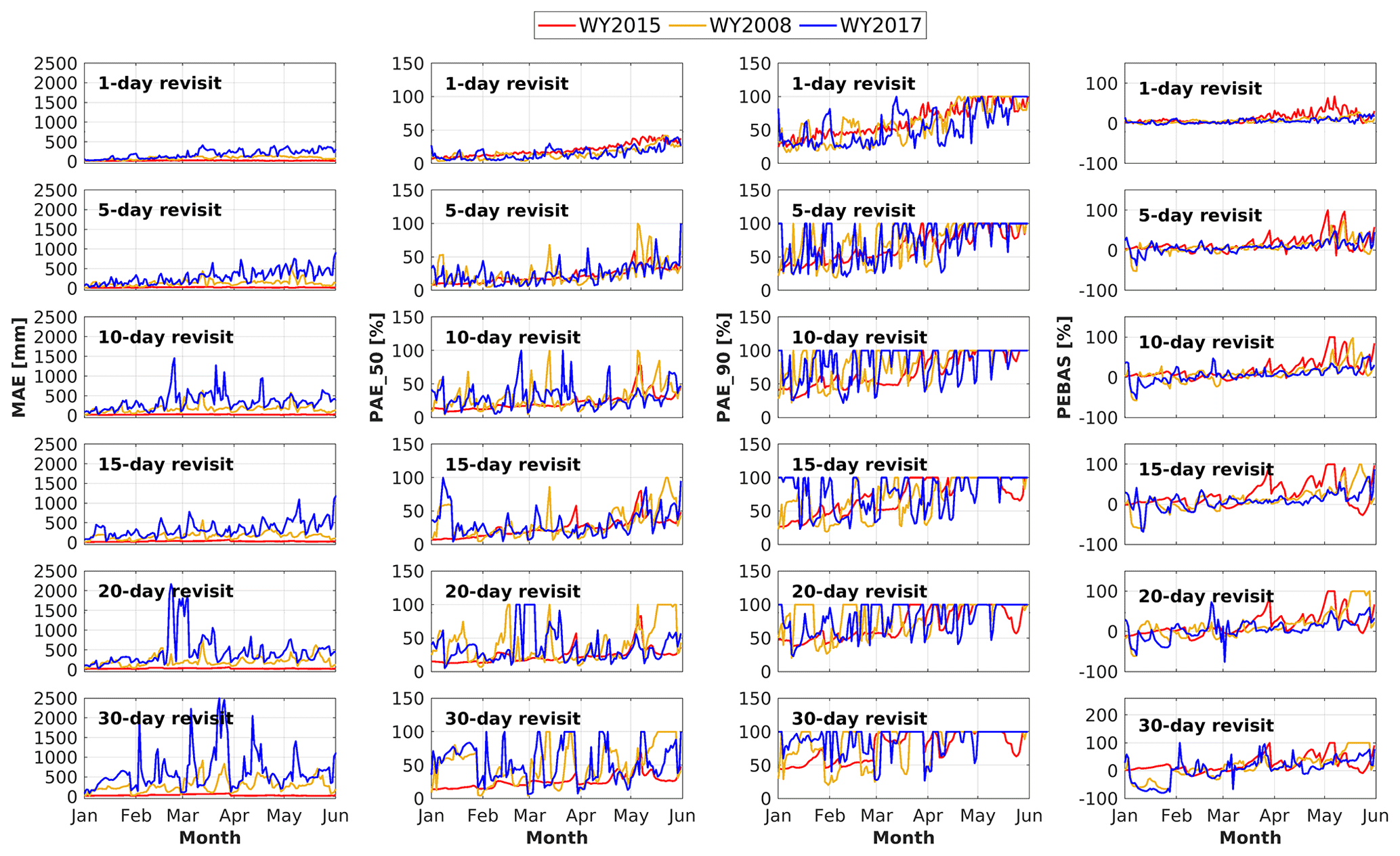
Figure 7 Daily time series of MAE (mm; first column), PAE_50 (%; second column), PAE_90 (%; third column), PEBAS (%; fourth column) from January to June in WY2015 (red line), 2008 (yellow line), and 2017 (blue line) based on revisit intervals of 1- through 30 d (rows 1–6, respectively).

The evolution of PAE_50, PAE_90 and PEBAS during the snow accumulation and snowmelt seasons (Fig. 7) shows that the errors increase with the time interval between overpasses. Differences in accuracy for time intervals up to about 15 d are not apparent, despite slight underestimation at the beginning of January and overestimation near the end of May (especially for the normal year) but becoming more apparent with longer time intervals. For most days during snow accumulation and snowmelt periods, the values of PEBAS and PAE_50 are less than 30 %. Assuming a 10 d overpass interval, percent errors in basin-averaged SWE are mostly less than 10 %. However, as the overpass interval increases beyond 20 d, the values of PEBAS and PAE_50 exceed 50 % for most of the days from January to June. Also, the underestimates at the beginning of the snow accumulation season and overestimates at the end of the snowmelt period are much more apparent for overpass intervals exceeding 20 d. From the perspective of PAE_90, except for the 1 and 5 d revisit scenarios, the values of PAE_90 are mostly larger than 50 % from January to June. This is probably because there are many low SWE pixels during snow accumulation and snowmelt seasons in addition to the days near the time of peak SWE. With the longer time interval, the ability of SWE estimation degrades, so that more than 10 % of the pixels (most of them are low-SWE pixels) in the study area have large percent absolute errors despite different climate conditions.

Considering revisit intervals from 1 to 30 d, in general 5, 10 and 15 d intervals are plausible options that balance revisit frequency and estimation accuracy. The 1 d interval does not improve the results much, relative to, for instance, 5 d, but performance for greater than 20 d revisits is substantially degraded.

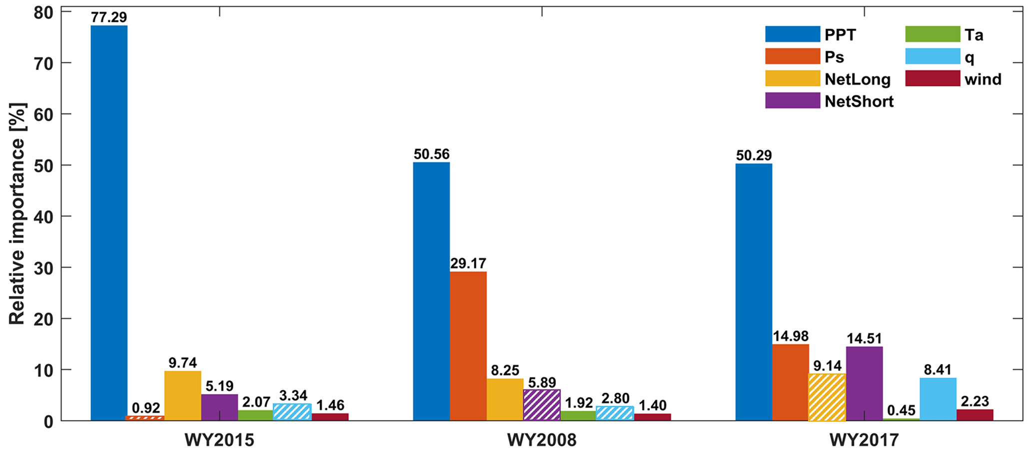
Figure 8 Relative importance (%; normalized values of absolute change of MAE after removing one forcing field) of each meteorological forcing in DNN-based full-domain SWE estimates in WY2015, WY2008 and WY2017. The bars with dashed lines indicate that removing those variables decreases the value of MAE, while solid bars indicate that removing those variables increases MAE.

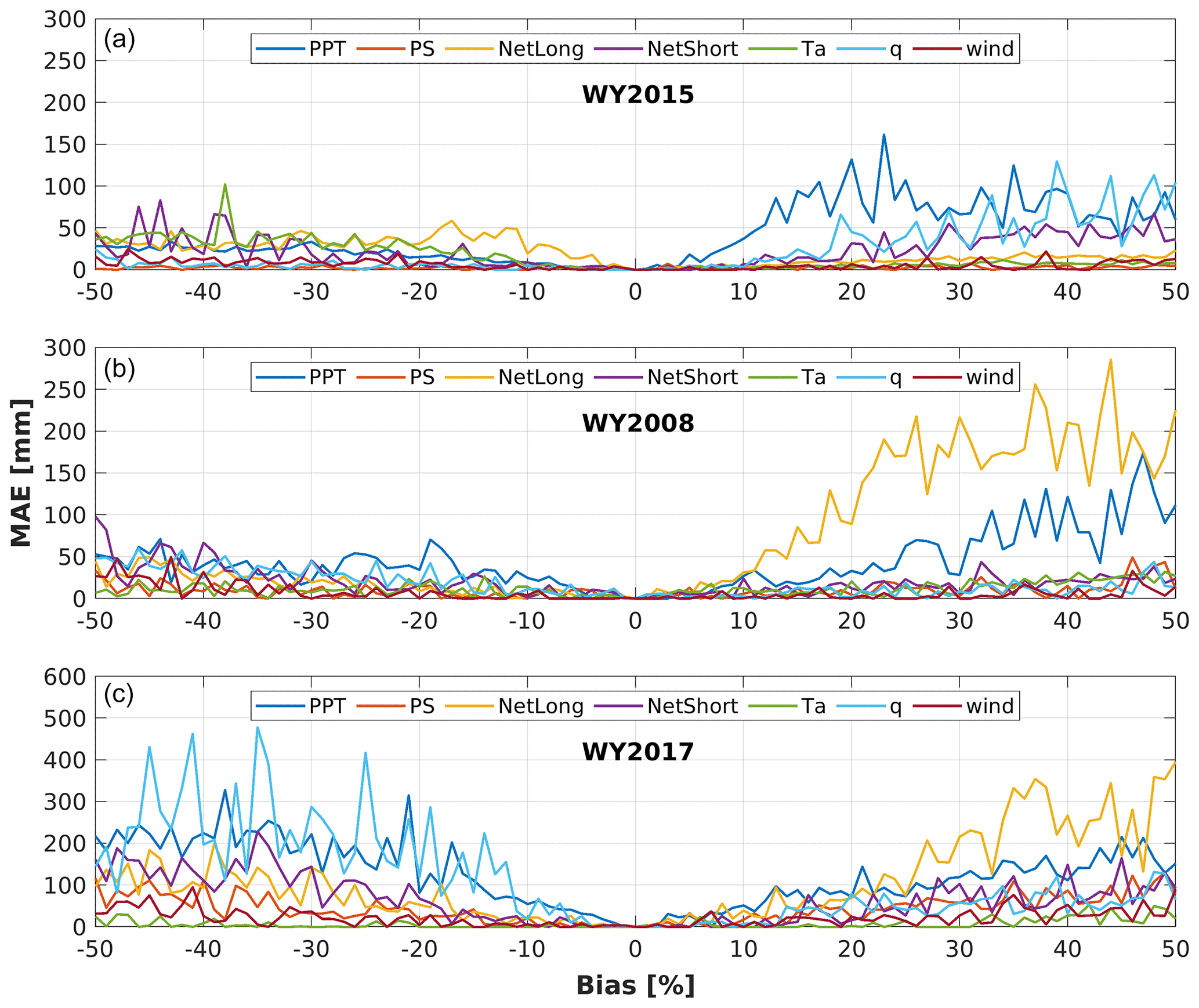
Figure 9 Changes of MAE (mm; relative to no bias) of the inferred 1 April SWE in WY2015 (dry year; first row), WY2008 (normal year; second row) and WY2017 (wet year; third row) with biases perturbed in the meteorological forcings of the training datasets. The limit of the y-axis scale in the WY2015 panel is smaller than that of WY2008 and WY2017 to make the small MAE in WY2015 discernible.

4.3 Input feature sensitivity test

The missing feature analysis evaluates the relative influence of each forcing field on the estimation of domain-wide SWE (Fig. 8). In general, winter precipitation is the most influential of the meteorological forcings in SWE estimation (Raleigh and Lundquist, 2012; Luce et al., 2014). The results show that in the dry, normal and wet years, precipitation is the dominant variable with relative contributions exceeding 50 % (WY2015: 77.3 %; WY2008: 50.6 %; and WY2017: 50.3 %), confirming that precipitation is the variable that provides the most useful information for establishing the DNN-based TTA relationship, regardless of climate conditions. The dominance of precipitation is most significant in WY2015 with thinner snowpacks, the longevity of which is more sensitive to winter precipitation than in wetter years. In addition to precipitation, long-wave radiation and short-wave radiation also play important roles in the domain-wide SWE estimation due to their critical controls on snowmelt rate and timing. We noticed that the occasional removal of a particular meteorological forcing inversely increased MAE (e.g., q in WY2015 and WY2018, NetShort in WY2008, and NetLong in WY2017). This is probably because these meteorological variables do not play an important role in the corresponding years and including the information of such variables would bring noises to the ML system and therefore deteriorate the performance of the TTA SWE transformation. For example, the influence of q was negligible, and sometimes q has been assumed to be constant in previous snow modeling (e.g., Cline et al., 1998; Clark et al., 2011) and Netlong and NetShort may only provide limited information for SWE modeling as the winter precipitation is relatively abundant (e.g., Clark et al., 2011).

The changes of model performance as a result of the error perturbation in the training dataset (Fig. 9) show the potential influence of forcing biases on the SWE estimation results in the dry year (WY2015), normal year (WY2008) and wet year (WY2017). We explored the sensitivities of DNN-based (which is the best TTA transformation method) domain-wide SWE estimation results to different levels of biases perturbed to the training dataset. Figure 9 shows two points. First, the bias in the training meteorological features propagate to the SWE estimates, especially in the years with normal and deep snow, which is not surprising because the bias affects the model training and larger biases have larger impacts. Second, the fluctuation in each MAE curve in Fig. 9 is obvious. The reasons for the fluctuation in the curves are as follows: (1) Every time we add biases to the training meteorological data, we need to re-train the DNN-based TTA relationship. The weights assigned for each neuron in each hidden layers in DNNs have a degree of randomness, so even though the object of every DNN is to achieve the optimal estimation results, the inner structure of the DNNs are different to adapt to the biased training dataset. (2) We only use 85 % of training data that are randomly split from the original dataset (the remained 15 % are used for model test). With different training data, each time we obtain a different DNN, so SWE estimates from the network are slightly different.

In the extremely dry year (WY2015), the DNN-based domain-wide SWE estimates are not sensitive to the biases in the meteorological training inputs (Fig. 9), likely due to its extremely low snow cover. Among the seven meteorological forcings, T_a (primarily the positive biases of T_a) has relatively larger impacts on the accuracy of SWE estimates than the other meteorological forcings in WY2015. In the normal (WY2008) and wet (WY2017) years, positive biases of long-wave radiation and negative biases of precipitation are the main sources of DNN-based SWE estimate errors (Fig. 9). In the years with relatively abundant precipitation (normal and wet years), precipitation is highly positively correlated with SWE values, so any precipitation errors in the training dataset can have a large impact on the accuracy of SWE estimation. In addition, we propose the following possible reason for the larger MAE caused by positive errors rather than negative errors: essentially decreasing long-wave radiation cannot increase 1 April SWE above the accumulated snowfall, but increasing long-wave radiation can decrease SWE all the way to zero (in theory), so increased net long-wave radiation influences the SWE estimates more than a decrease thereof (Sicart et al., 2006). In the DNN-based SWE estimates, errors in air pressure (P_s), air temperature (T_a), specific humidity (q), net short-wave radiation (NetShort) and wind speed (wind) have very small impacts on domain-wide SWE estimation under normal or wet climate conditions.

The robustness and stability of SWE estimate models are critical to estimating full-domain SWE in real applications. Overall, the performance of DNN degrades with more biases added to the training meteorological inputs in the normal and wet years, while the dry year is less sensitive to biases in the training data. Despite the fact that forcing biases can lead to lower SWE estimation accuracy in the normal and wet years, DNN-based SWE estimation has MAE <300 mm when the biases in training forcings are as large as ±50 %, indicating the robustness of DNN in the TTA SWE transformation. The feature sensitivity results for the other three methods (MVLR, RF and SVM) in the dry, normal and wet years are shown in Fig. S4–6.

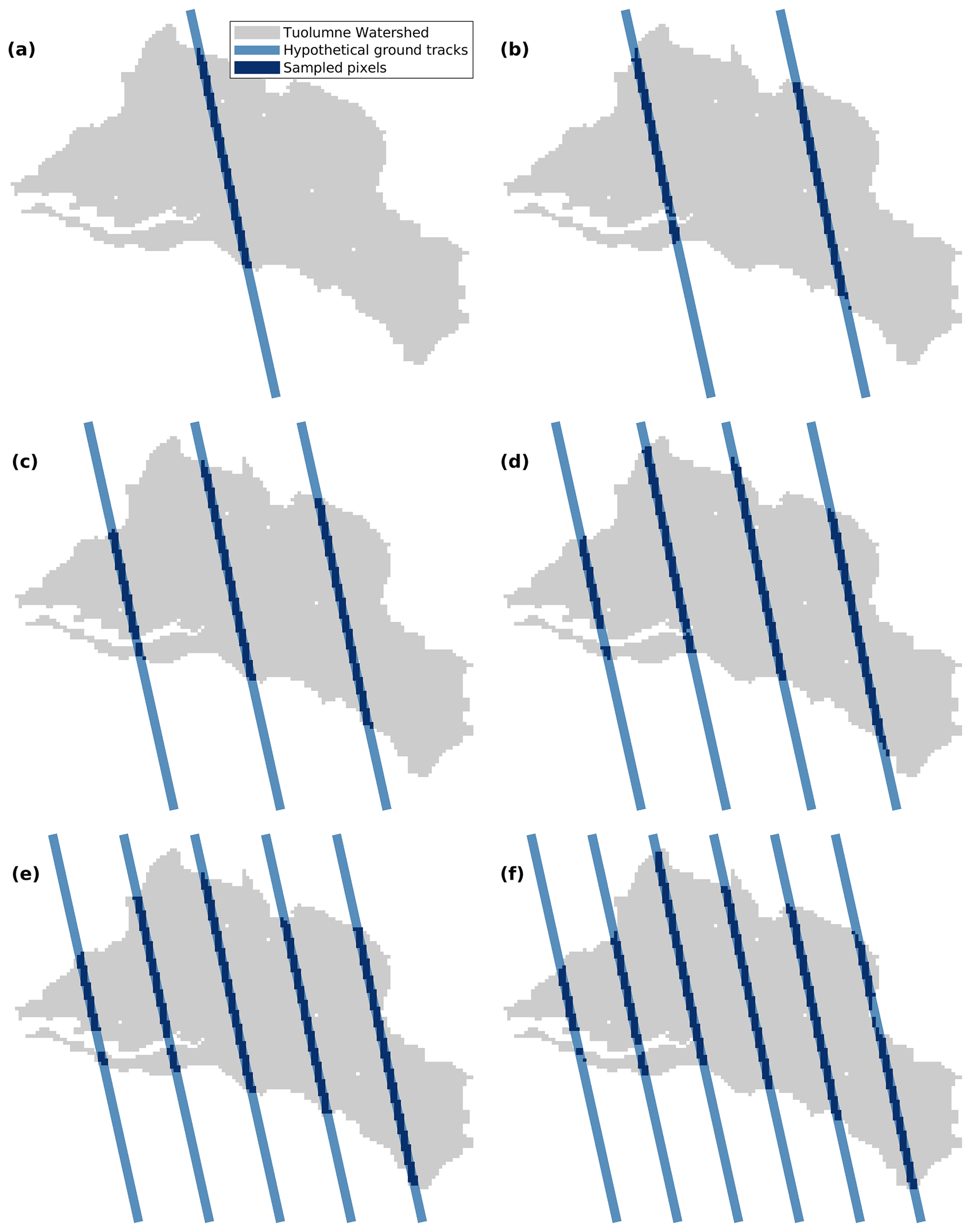
Figure 10 Illustration of the 1–6 (a–f, respectively) hypothetical ground tracks in the upper Tuolumne watershed. The distance between each track is roughly the same over the whole watershed.

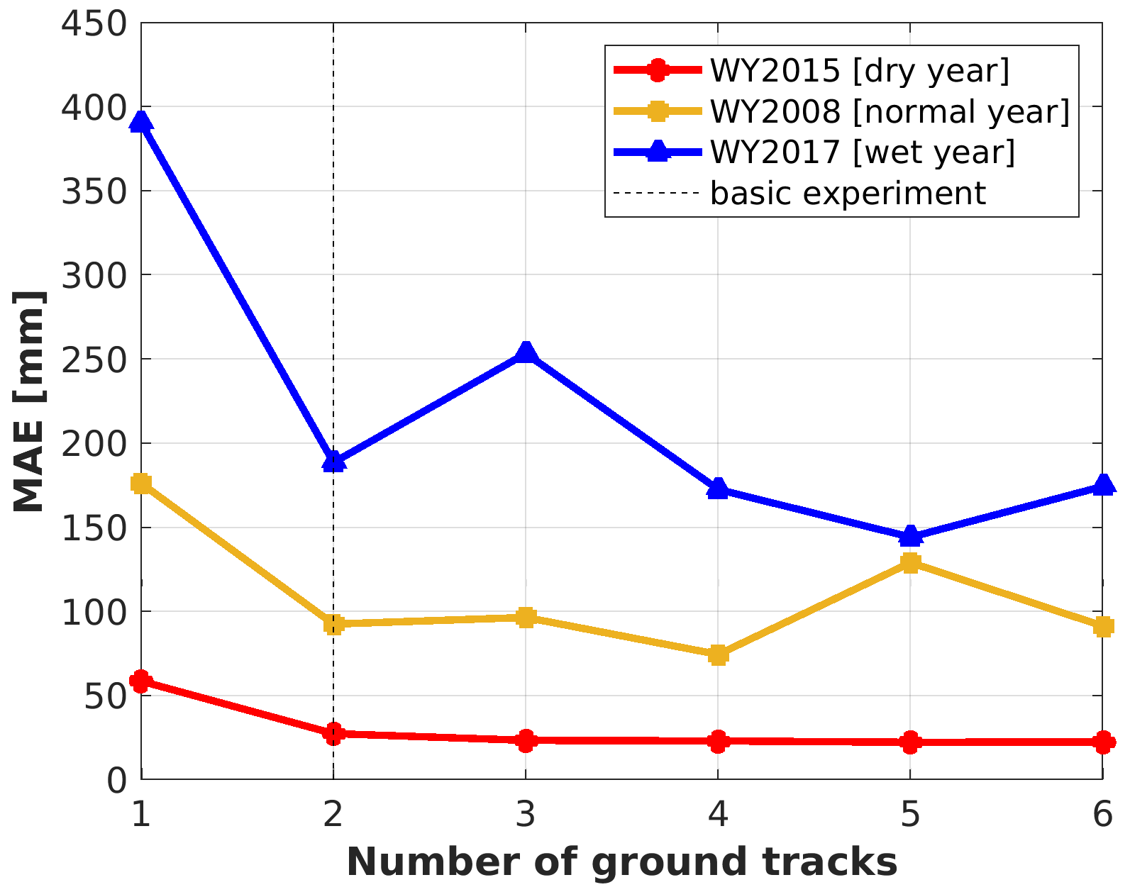
Figure 11 Changes in MAE (mm) of the DNN-based inferred 1 April SWE in dry (WY2015; red dots), normal (WY2008; yellow square points) and wet years with the number of ground tracks. The dashed lines for the number of ground tracks equal to 2 indicate that the addition of more satellite overpasses do improve the estimates much (see also Sect. 4.1).

4.4 Sensitivity of TTA to the number of ground tracks

Figures 10 and 11 show the changes in MAE of the domain-wide 1 April SWE estimates with different numbers of ground tracks. We compared the SWE estimation errors in the dry, normal and wet years (i.e., WY2015, 2008, 2017, respectively) using the DNN-based TTA method. In general, the performance of the DNN-based domain-wide SWE estimates improve with more ground tracks in the 3 years (Fig. 11). The improvement in the domain-wide SWE estimation is most distinct in the wet year, probably because more information for building the TTA relationship is available when snow accumulation is larger, and the number of pixels with zero or nearly zero SWE is smaller.

Statistically, in WY2015, DNN estimates the basin-wide 1 April SWE with MAE less than 40 mm when two or more ground tracks are available. Similarly, in WY2008 (a normal year), the DNN method has MAE less than 100 mm with two or more ground tracks. In all years, improvements in accuracy are small when the number of tracks exceeds two.

Regardless of snow climatologic conditions, the improvements of TTA performance with additional overpasses are limited when the number of ground tracks is larger than or equal to two. Based on the elevation distribution of pixels on synthetical ground tracks (Fig. S7), if more than two ground tracks pass through the study area, the useful information added to the training data become limited since pixels at different elevation bands seem to be similarly distributed, thus the decrease of MAE is limited. Also, the decrease of MAE as the number of the ground tracks increases from one to two could likely benefit from the addition of training data in low-elevation regions (elevation <2500 m). Considering the trade-off between SWE estimation accuracy and the cost of additional overpasses, one or two ground tracks is likely the optimal choice for purposes of domain-wide SWE estimation. It is noticeable that topography plays an important role in the performance of TTA SWE transformation. The MAE increases in the course of the number of ground tracks added from two to threee in the wet year and the number of ground tracks increases from four to five in the normal years. The reason for the outliers is probably because in the wet and normal years, as there are more than or equal to two ground tracks in the study area, the topography over ground tracks is enough to represent the situations over the whole basin. Under such circumstances, the increase in the number of ground tracks can increase the training size but therefore involves more training samples with biased conditions.

The DNN-based SWE estimation is more accurate than the other methods regardless of the size of the training dataset and the climate conditions. In contrast, the statistical method is the worst of the four (Fig. S8).

5 Conclusions

Spatially continuous SWE estimates are of key importance to the prediction of the timing and volume of streamflow in snow-dominated regions. The potential now exists via at least two satellite-based technologies to measure SWE along tracks, which would cover only a small portion of a watershed's area. Fortunately though, relationships exist among multiple accessible variables (static and forcing fields) and SWE that can be used in linear or non-linear relationships to fill the gaps between tracks. Here, we use statistical and machine learning methods that are trained using the static variables, meteorological forcings and SWE observations along tracks to estimate SWE over the entire domain (watershed). We tested (1) how the relationship between the training inputs and SWE along ground tracks could be used to infer SWE across the entire basin, (2) the performance of four algorithms applied over a full water year, (3) the influence of biases in meteorological forcings of the training dataset on the accuracy of the MVLR and three ML methods, and (4) changes in model performance with various numbers of overpasses. We focused on estimate accuracy over the upper Tuolumne watershed during dry (WY2015), normal (WY2008) and wet years (WY2017). Based on our results, we conclude the following:

1. It is possible to derive basin-wide peak SWE (on 1 April) with high accuracy (on the basis of MAE, PAE_50, PAE_90 and PEBAS) when the interval between satellite revisits is in the 5–10 d range.

2. The DNN method is the most accurate of the four we tested regardless of snow climatological conditions. The DNN is also the most robust method with respect to biases in forcing data and reduction in the training data size. Though the DNN employed here is a simple MLP, it outperforms the statistical and the other two ML methods. It is reasonable to expect further improved performance of DNN with better network structure and hyper parameter optimization in future applications of snow data retrieval.

3. Based on missing feature analysis, precipitation is the dominant variable in domain-wide SWE estimation, especially in dry years. According to the results of our feature uncertainty analysis, the biases of precipitation and the net long-wave radiation have the greatest influence on the accuracy of domain-wide SWE estimation.

4. As the number of ground tracks crossing the domain increases, the MAE of the inferred 1 April SWE improves, but only modestly when the number of ground tracks is more than two.

Our work demonstrates the feasibility of using ML algorithms (which almost always were more accurate than MVLR) to achieve TTA SWE estimates. Operationally, our feature sensitivity experiment provides a basis for determining the focus of quality control of meteorological forcings and the corresponding selection of TTA transformation methods. Furthermore, our exploration of the effects of addition of overpasses suggests the preferred balance between estimation accuracy and the number of satellite tracks: for the most part, increases in estimation accuracy are modest for more than two tracks. Further research could consider the improvements of ML algorithms to improve the stability, efficiency and accuracy of the TTA transformation systems. Lastly, due to the availabilities of the training datasets and accurate short-term forecast of meteorological conditions (∼1–2 weeks ahead), our ML methods can be used beyond the TTA framework for a history-to-future (HTF) snow estimation, where a trained relationship between historical snow and forcing fields across an area can be used in conjunction with the short-term meteorological forecasts to accurately forecast the SWE condition over the domain.

Finally, we assumed a spatial resolution of satellite SWE observations to be 1 km, which is now technically feasible. However, higher spatial resolutions seem likely in the future. In the context of our experiments, higher spatial resolution would increase the training size of the ML-based TTA SWE transformation, which likely would lead to better performance of continuous SWE estimation. Future research might therefore explore the extent to which TTA performance would benefit from higher spatial resolution in the context of the trade-off between increased training size and ML-based estimation accuracy.