Hydrologic implications of projected changes in rain-on-snow melt for Great Lakes Basin watersheds

Rain-on-snow (ROS) melt events reduce the amount of water stored in the snowpack while also exacerbating flooding. The hydrologic implications of changing ROS events in a warming climate, however, are still uncertain. This research used a calibrated and validated Soil and Water Assessment Tool (SWAT) hydrologic model, modified with energy budget equations to simulate ROS melt and forced with a climate model ensemble representing moderate greenhouse gas concentrations, to simulate changes to ROS melt in the North American Great Lakes Basin from 1960–2069. The changes to ROS events between the historic period (1960–1999) and mid-century (2040–2069) represent an approximately 30 % reduction in melt in warmer, southern subbasins but less than 5 % reduction in melt in colder, northern subbasins. Additionally, proportionally more rainfall reduces the formation of snowpacks, with area-weighted combined winter and spring rain-to-snow ratios rising from approximately 1.5 historically to 1.9 by the mid-21st century. Areas with historic mean combined winter and spring air temperatures lower than −2 ^∘C have ROS regimes that are resilient to mid-21st century warming projections, but ROS occurrence in areas that have mean combined winter and spring temperatures near the freezing point are sensitive to changing air temperatures. Also, relationships between changes in the timing of ROS melt and water yield endure throughout spring but become weak by summer. As the influence of ROS melt events on hydrological systems is being altered in a changing climate, these conclusions are important to inform adaptive management of freshwater ecosystems and human uses in regions of the globe that are sensitive to changes in ROS events.

1 Introduction

Rain-on-snow (ROS) melt events can have important implications for winter floods because of the combined impacts of rainwater and snowmelt runoff (Suriano and Leathers, 2018; Leathers et al., 1998). In places where ROS events are common, they have contributed to the majority of extreme floods, including locations in the United States northwest, upper Midwest, northeast, and Appalachians (Li et al., 2019). ROS events can occur across a wide swath of North America and Eurasia in areas that have substantial snowpack (Pomeroy et al., 2016; Rennert et al., 2009; Rössler et al., 2014; Sui and Koehler, 2001; Ye et al., 2008; Musselman et al., 2018), but their impact on hydrology extends beyond the cold season because snowpack conditions throughout the winter and spring influence the availability of groundwater and stream water later in the year (Blahušiaková et al., 2020; Jenicek et al., 2016; Myers et al., 2021b). Compared to thermally driven snowmelt rates, rainfall-based melt events are often more short-lived and intense. As a result, ROS melt produces proportionally more runoff compared to temperature-based snowmelt, with lower rates of infiltration and groundwater recharge (Wilson et al., 1980; Earman et al., 2006). Thus, ROS melt events can lead to snow droughts and reduced water availability after the snow season because of the lost water storage (Harpold et al., 2017; Hatchett and McEvoy, 2018; Blahušiaková et al., 2020; Myers et al., 2021b).

In the North American Great Lakes Basin, ROS melt is associated with over 25 % of the most extreme snowmelt events (Suriano, 2020) and has been shown to influence hydrological droughts later in the year (Myers et al., 2021b). ROS events melt an average of 4 cm of snow per event in the Great Lakes Basin but decreased in frequency by 37 % from 1960–2009 (Suriano and Leathers, 2018). ROS melt typically occurs when a midlatitude cyclone takes a more northerly track, transporting warm, moist air into the basin (Suriano, 2018). At the same time, the snow water equivalent (SWE) available in the snowpack is critical, and average snow depths in the basin decreased by 25 % from 1960–2009 (Suriano et al., 2019). However, the hydrological impacts of changing ROS melt amounts and frequencies in a transient climate are uncertain, as a decrease in snowpack could not only limit the amount of ROS melt but also increase surface runoff from rain on bare ground during cold seasons.

This research combines outputs from an ensemble of downscaled climate models with a version of the Soil and Water Assessment Tool (SWAT) hydrologic model (Arnold et al., 1998) that incorporates a ROS melt modification (Myers et al., 2021b) to simulate climate change impacts to watersheds in the Great Lakes Basin. Our research asks the following: “how does ongoing climate change alter ROS melt and hydrology in the Great Lakes Basin by the mid-21st century?” This research contributes to scientific knowledge by advancing our understanding of climate change impacts to watersheds, particularly concerning the impacts of ROS melt, thereby improving our ability to manage water quantity and quality into the future. It is important to understand these climate change impacts to sustainably manage rivers and prepare for risks, both within the Great Lakes Basin and in ROS-prone regions around the world.

2 Materials and methods

2.1 Study area

The North American Great Lakes Basin is the Earth's largest fresh surface water system (Environment Canada and USEPA, 1995), including portions of eight USA states and one Canadian province (Fig. 1). To the north, near Lake Superior, snow cover lasts an average of 180 d but is as low as 107 d around Lake Erie (Suriano et al., 2019). The Great Lakes Basin is experiencing a rapidly changing climate (Lehner et al., 2006; Environment Canada and USEPA, 1995), with average annual air temperatures having already risen nearly 1 ^∘C since the early 20th century, while annual total precipitation has risen approximately 10 % (Wuebbles et al., 2019).

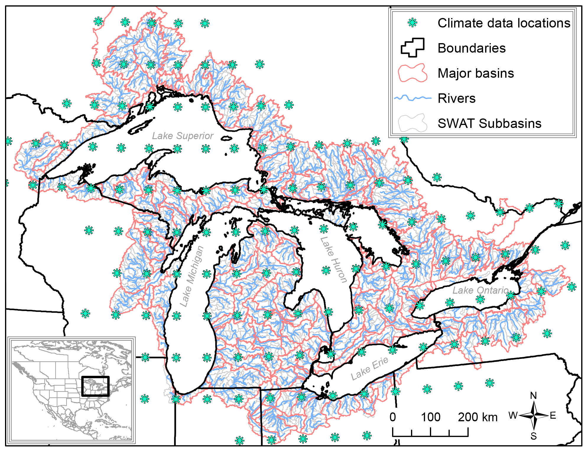
Figure 1 Study area map of the Great Lakes Basin, showing historical and projected climate data grid points and study river systems.

2.2 Hydrology simulation

We used the SWAT hydrological model (Arnold et al., 1998) with a modified snowmelt routine to simulate ROS melt. SWAT simulates hydrology with a water balance of inputs (precipitation), exports (evapotranspiration, surface runoff, groundwater flow, and lateral flow), and soil water storage. SWAT partitions precipitation into rainfall or snowfall, based on whether the air temperature is above or below a temperature threshold (Fontaine et al., 2002). Groundwater flow was simulated with a shallow aquifer water balance, and evapotranspiration was simulated using the Penman–Monteith method (Monteith, 1965; Ritchie, 1972).

A full description of the ROS modification, hydrology simulation, calibration, and evaluation can be found in Myers et al. (2021b). In short, the SWAT source code was modified to include an energy budget equation for snowmelt from the SNOW-17 model (Anderson, 1973, 2006) that simulates ROS melt based on a function of air temperature, precipitation, wind, saturated vapor pressure, and atmospheric pressure. For the SWAT ROS model, air temperature and precipitation are based on existing SWAT model inputs, wind effects on ROS are simulated using an average function for ROS melt from turbulent energy transfer, saturation vapor pressure is based on air temperature, and atmospheric pressure is based on elevation, so no additional data inputs are required. Previously, SWAT would simulate snowmelt using a snowpack temperature that was based on air temperature (Fontaine et al., 2002), which would not consider daily ROS melt events. Using a snowmelt module that can simulate ROS melt, such as our SWAT ROS model, reduces error and leads to more accurate hydrological simulations in the Great Lakes Basin due to the more accurate simulation of the timing of snowmelt (Myers et al., 2021b).

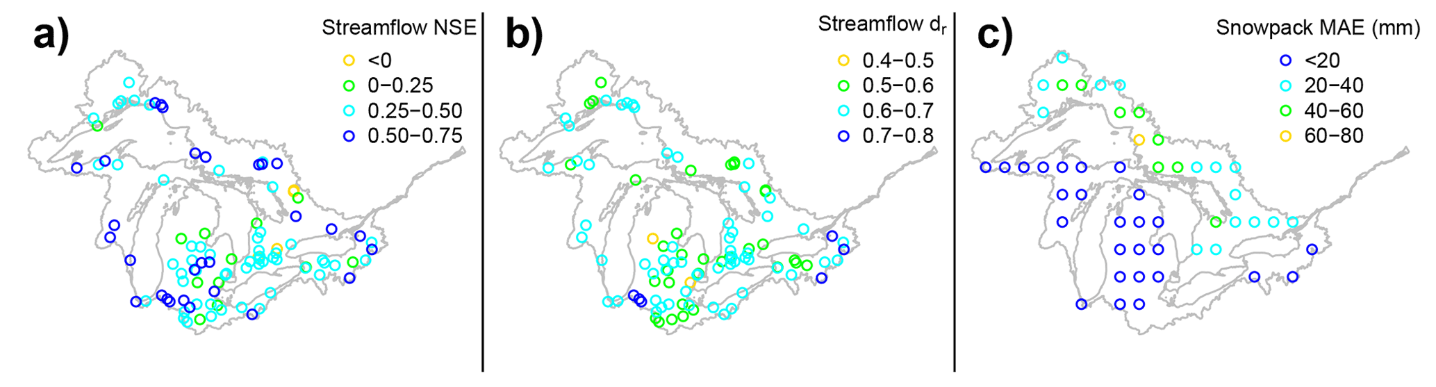
Figure 2 Evaluation statistics for simulating historic streamflow and snowpack. (a) Streamflow using the Nash–Sutcliffe efficiency (NSE). (b) Streamflow using the revised Index of Agreement (d_r). (c) Snowpack using the mean absolute error (MAE) at the daily time step. This figure has been adapted from Myers et al. (2021b).

This study used a calibrated version of the SWAT hydrological model for the Great Lakes Basin previously developed in Myers et al. (2021b), based on historic climate inputs (Maurer et al., 2007). In Myers et al. (2021b), a sensitivity analysis was performed using the PAWN method (Pianosi and Wagener, 2015) that identified 24 sensitive parameters. The model was then calibrated at the daily time step with the algorithm called a multialgorithm, genetically adaptive multiobjective method (AMALGAM; Vrugt and Robinson, 2007), using 99 stations for streamflow and 50 stations for snowpack snow water equivalent (SWE). SWE was estimated from the gridded North American snow depth dataset (Mote et al., 2018), using a function of snow depth, precipitation, temperature, and time of year (Hill et al., 2019). The Nash–Sutcliffe efficiency (NSE; Nash and Sutcliffe, 1970) and the revised Index of Agreement (d_r; Willmott et al., 2012) were the objective functions for streamflow, while the mean absolute error (MAE; Willmott and Matsuura, 2005) was the objective function for snowpack SWE.

The SWAT ROS model for the Great Lakes Basin simulated historic streamflow at the daily time step, with an average NSE of 0.38 (with 29 % of stations greater than 0.5, 48 % greater than 0.4, and a maximum NSE of 0.71) and an average d_r of 0.62 (Myers et al., 2021b). Stations with streamflow NSE > 0.50 at the daily time step were spread throughout the Great Lakes Basin, suggesting that the model was representative of the spatial tendencies in climate forcings and hydrological responses (Fig. 2a). Stations that performed well with d_r>0.60 were also distributed across the basin, which is important because d_r is not as influenced by extremes as NSE (Willmott et al., 2012) and can be a more interpretable indicator of overall model performance (Willmott et al., 2015). Furthermore, the presence of stations not performing as well by the NSE could be at least partly explained by the diversity of spatially distributed hydrological behaviors of the basin having been simplified in the model's multisite and multiobjective calibration (Zhang et al., 2008), in addition to uncertainties in gridded climate forcings (Maurer et al., 2010; Muche et al., 2020; Stern et al., 2022) and snowpack calibration data (Mote et al., 2018; Hill et al., 2019). Thus, we chose to focus on average amounts of ROS melt over different time periods for this study, without focusing on specific events such as extreme (e.g., 0.95 quantile) water yields. Those extremes may not be represented as reliably in future climate projections, given that many of the stations had lower NSE values than we deemed adequate for that purpose, largely because NSE values are sensitive to extremes (Legates and McCabe, 1999; Willmott et al., 2009). Furthermore, projections of climate change impacts on hydrologic extremes are best analyzed using models that focus on extreme flows specifically (Willems et al., 2014).

The model simulated historic snowpack SWE at the daily time step, with a MAE of 26 mm (Fig. 2a–c). Daily snowpack SWE error across the basin ranged from <20 mm MAE throughout the southwest subbasins to approximately 40–70 mm MAE in the northeast (Fig. 2c). This spatial variation in MAE scaled with the average observed daily snowpack SWE during winter and spring across the basin, which ranged from approximately 50–100 mm in the southwestern subbasins to over 150 mm in the northeast (described in Sect. 3.4). Thus, subbasins with lower amounts of observed SWE would also have smaller errors than the average of 26 mm. We find this measure of absolute error to be acceptable, particularly considering the errors inherent to the gridded snowpack data that we compare against (e.g., spatial averaging and simplification of accumulation and ablation processes during conversion from snow depth; Myers et al., 2021b; Ensor and Robeson, 2008; Hill et al., 2019). Mean absolute errors in modeling the gridded snowpack SWE have been found to vary temporally as well, for instance, being 12.7 mm MAE on 1 January, 45.1 mm MAE on 1 February, 26.8 mm MAE on 1 March, and 9.6 mm MAE on 1 April 1978 across the Great Lakes Basin in comparison with station measurements and proportional to the amount of snowpack on the ground during those days (Myers et al., 2021b). Previous work by Kalin et al. (2010) has stated that arbitrary interpretations of performance metrics for models at small temporal scales should be relaxed compared to what would be expected for models at coarse (e.g., monthly) time steps. Calibrated parameters for this model can be found in Table S1 in Myers et al. (2021b). We also investigated the seasonal model performance for simulating snowmelt (water equivalent) during only days when ROS melt was occurring and found that the SWAT ROS model we use had a MAE of 8.6, 9.4, and 5.8 mm for simulating snowmelt on those days in the winter, spring, and fall, respectively.

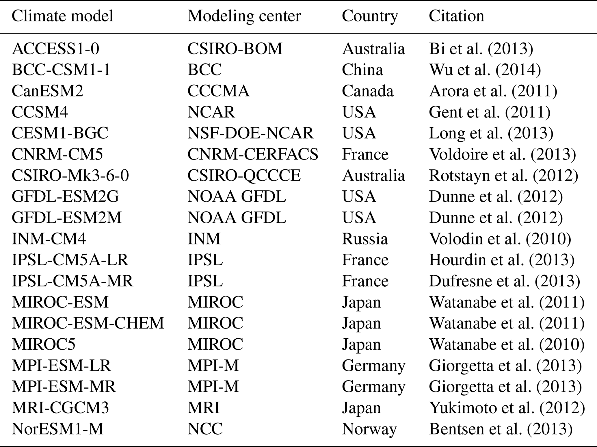
Table 1 Climate models for the Representative Concentration Pathway (RCP) 4.5 scenario used in the research. Full names for each modeling center can be found in Table S1 in the Supplement.

2.3 Climate projections

The calibrated hydrological model was forced with 1950–2099 climate projections from downscaled and bias-corrected outputs of the Coupled Model Intercomparison Project Phase 5 (CMIP5) multimodel ensemble (Taylor et al., 2012; US Bureau of Reclamation, 2013; Maurer et al., 2007). These models were downscaled to a 1^∘ latitude/longitude grid (Fig. 1) and bias-corrected using the Bias Correction and Constructed Analogs (BCCA) method (Maurer et al., 2010), which corrects bias by quantile mapping with historic data (US Bureau of Reclamation, 2013). A 1^∘ grid resolution was chosen for these projections because it matched the resolution of our snowpack data for calibration (Mote et al., 2018). It was important to have our snow data and climate projections at the same resolution so that we could calibrate the model for snow processes at the same scale as the response to air temperature and precipitation. These processes could be sensitive to differences between grids (Rajulapati et al., 2021; Winchell et al., 2013; Myers et al., 2021a).

Global climate models (GCMs) can be a major source of uncertainty when modeling the hydrological impacts of climate change (Wang et al., 2020; Chegwidden et al., 2019). Thus, 19 climate models for the Representative Concentration Pathway (RCP) 4.5 were used to account for variation in climate projections (Table 1). We chose to include 19 climate models because that was the total number of models using the RCP4.5 scenario that had been downscaled and bias-corrected in the multimodel ensemble (Maurer et al., 2007). RCP4.5 is a moderate greenhouse gas scenario that considers long-term changes in emissions, land cover change, the global economy, and climate change mitigation (Thomson et al., 2011). The mean of this multimodel ensemble was used to represent our projection (Christensen et al., 2010), with the standard deviation of the GCM ensemble shown in Fig. 3.

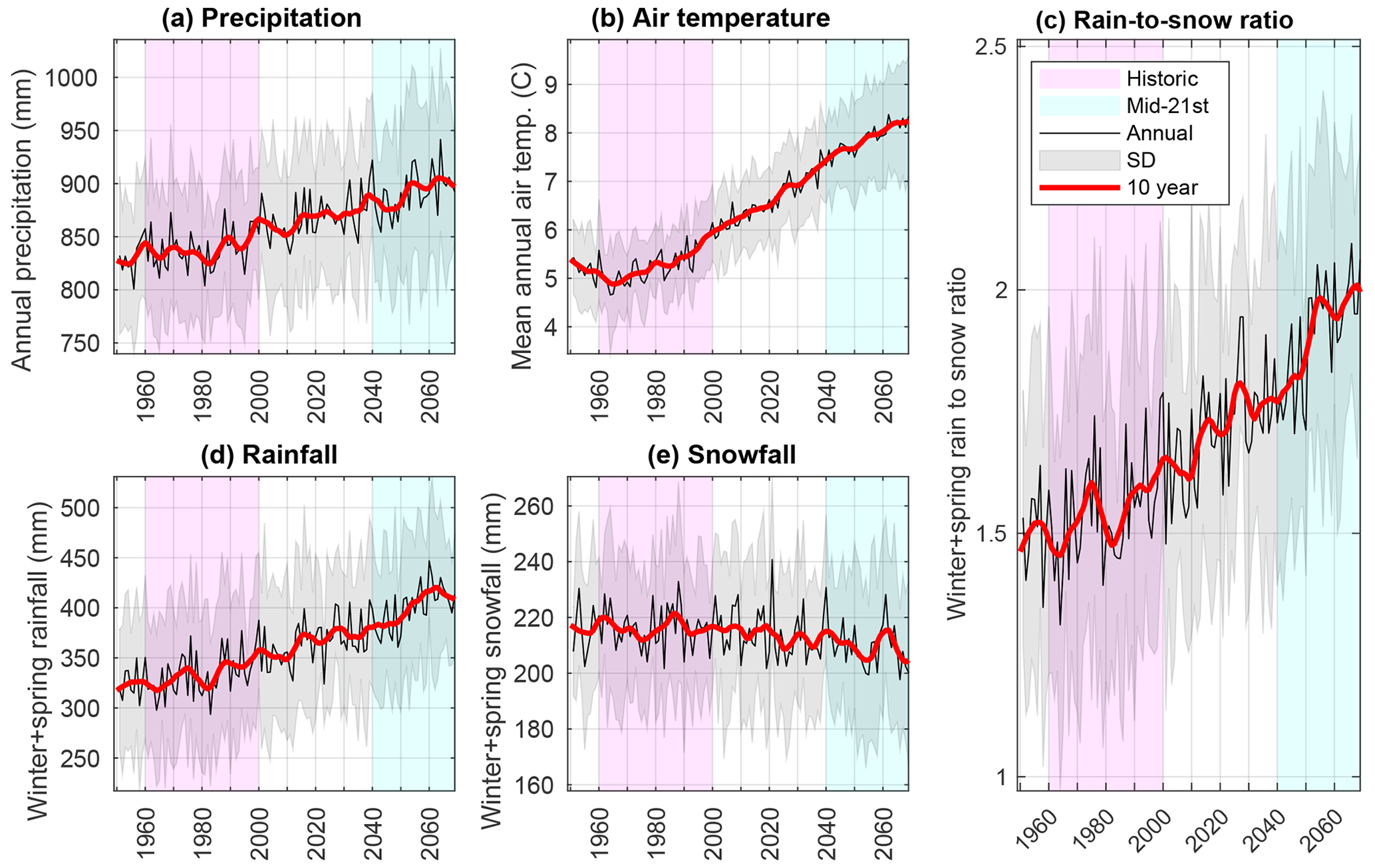
Figure 3 Basin-wide ensemble-averaged (a) annual total precipitation, (b) annual air temperature, (c) combined winter and spring rain to snow ratio, (d) combined winter and spring rainfall, and (e) combined winter and spring snowfall from the climate input data, with 10-year averages (red lines), based on the RCP4.5 pathway. Shading indicates historic (1960–1999; red) and mid-21st century (2040–2069; blue) periods, in addition to ensemble standard deviations (gray).

2.4 Analyses

Hydrological outputs from the SWAT model were aggregated to the boundaries of regulatory river basins for the USA (Hydrologic Unit Code (HUC) 8; USGS, 2022) and Canada (tertiary-level watersheds; Government of Ontario, 2022) using spatial averaging. Aggregating our subbasins into the regulatory major river basins from the USGS HUC 8 and Ontario tertiary-level watersheds data allowed us to compare SWAT outputs with the existing basin structure and facilitate the comparison and discussion of our results with other studies.

Results were analyzed by comparing the averages and extreme high events among historic (1960–1999) and mid-21st century (2040–2069) time periods at the subbasin scale, based on water years (1 October to 30 September). The mid-21st century period was the focus for informing water resources management and because of better agreement among the models. Simulations of ROS changes generally agree across CMIP5 RCPs (4.5 and 8.5) until the mid-century but then diverge by the late century (Musselman et al., 2021a). Calculations of basin-wide averages were weighted by subbasin area. Seasons were defined as winter (December, January, and February), spring (March, April, and May), summer (June, July, and August), and fall (September, October, and November). ROS melt events were defined as days with >1 mm rainfall on >1 mm snowpack SWE and snowmelt occurring, which is a definition that has been previously used to model ROS events and project climate change impacts (Jeong and Sushama, 2018). The ROS center of volume statistic, defined as the day of the water year when half the total volume of ROS melt has passed, was used to examine changes to the timing of ROS melt events (adapted from Hodgkins et al., 2003).

Pearson's correlation was used to evaluate the strength of the linear relationships, with significant relationships defined as p<0.05. For comparisons between time periods, statistical significance was evaluated by comparing the annual area-weighted ensemble-averaged values for the Great Lakes Basin between the historic (1960–1999; n=40 years) and mid-21st century (2040–2069; n=30 years) periods using two-tailed unpaired t tests. Box plots and percentiles were spatially weighted by major river basin area (Willmott et al., 2007). Finally, the SWAT model outputs for water yield represent the area-averaged water export through the outlet (in mm).

3 Results

3.1 Precipitation and air temperature projections

Across the Great Lakes Basin, the CMIP5 ensemble average annual precipitation and air temperatures are projected to increase between the historic (1960–1999) period and mid-21st century using RCP4.5. Spatially averaged annual precipitation increases by 53 mm (6.3 %) from 839±63 mm (mean and standard deviation of GCM ensemble) during 1960–1999 to 892±77 mm by the mid-21st century (p<0.001), while spatially averaged annual air temperatures increase 2.7 ^∘C from 5.2±0.7 ^∘C during the 1960–1999 period to 7.9±1.0 ^∘C (p<0.001; Fig. 3a and b). Changes in ensemble mean combined winter and spring air temperatures are most prominent in northern parts of the basin, where combined winter and spring air temperatures are projected to rise approximately 3 ^∘C between the historic (1960–1999) period and mid-21st century, using the RCP4.5 scenario (Fig. 4a and b). Using the GCM ensemble mean, changes in mean combined winter and spring rainfall are strongest in the Lake Superior region, where the amount of rainfall is projected to increase over 40 % (Figs. 4c–d and 3d). Northern areas experience the least change in ensemble mean combined winter and spring snowfall amount between the historic (1960–1999) period and mid-21st century, while southern parts of the basin have a decrease in snowfall over 10 % (Figs. 4e–f and 3e). Furthermore, our model shows that combined winter and spring rain-to-snow ratios over the basin (calculated by dividing the total combined winter and spring rainfall by total combined winter and spring snowfall) increase from around 1.5 historically to 1.9 by mid-century (p<0.001), which means that proportionally more rainfall could contribute to the declines in snowmelt and snowpack SWE (Fig. 3c).

Figure 4 Historic and projected climate changes for the Great Lakes Basin between the historic (1960–1999) period and mid-21st century (2040–2069) for RCP4.5 ensemble mean combined winter and spring. (a, b) Air temperatures. (c, d) Rainfall. (e, f) Snowfall. Each of these categories is based on water years. (a, c, e) Historic amounts. (b, d, f) Absolute or percent changes.

3.2 Snowpack and snowmelt projections

Between the historic (1960–1999) period and mid-21st century, winter months generally see an increase in the amount of ROS melt for individual subbasins due to the increased amount of rainfall (not snowfall) under RCP4.5 projections. For instance, the area-weighted median (value of a ranked set, where half of the total area is ranked lower; Willmott et al., 2007) amount of January ROS melt among subbasins increases 59 % from 3.2 mm historically to 5.1 mm by mid-21st century (Fig. 5a). Similarly, area-weighted median February ROS melt rises 50 % from 7.0 mm historically to 10.5 mm in the mid-21st century. In the spring, the amount of ROS melt decreases due to the reduction in snowpack. For instance, the area-weighted median amount of April ROS melt among subbasins decreases 56 % from 52.3 mm historically to 22.9 mm by the mid-21st century.

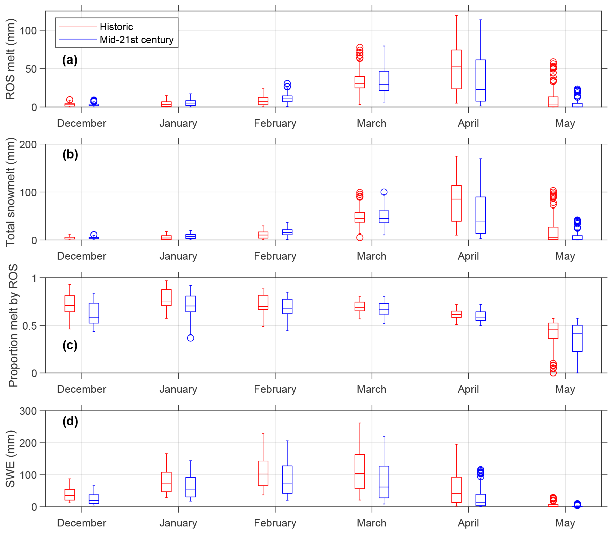
Figure 5 Changes in RCP4.5 ensemble mean monthly (a) rain-on-snow (ROS) melt, (b) total snowmelt (including temperature-based melt and ROS), (c) the proportion of monthly snowmelt from ROS events, and (d) snowpack snow water equivalent (SWE) for 158 individual major river basins of the Great Lakes Basin between the historic (1960–1999) and mid-21st century periods. Box plots display the median and interquartile range of results for major river basins and are weighted by river basin area (Willmott et al., 2007).

Mean monthly snowmelt (including temperature-based melt and ROS melt) among individual Great Lakes Basin subbasins is projected to experience a decrease and shift to earlier timing in the spring by the mid-21st century (Fig. 5b) using the RCP4.5 pathway. Historically, the maximum snowmelt overall has been in April, with an area-weighted median of 85.3 mm, while the March median snowmelt has been less at 44.8 mm. By the mid-21st century, the median amount of monthly snowmelt among subbasins reaches a maximum at 44.8 mm in March but drops to only 39.5 mm in April, which is a 54 % decrease during April between the two periods.

Changes in the amount of monthly snowmelt among individual subbasins are affected by changes to ROS melt amounts because days that have ROS melt occurrences account for more than 50 % of the total snowmelt for most subbasins from December through April (Fig. 5c). Temperature-based snowmelt is usually a slower process, while ROS melt events combined with temperature-based melt on these days can rapidly melt snowpack. However, the proportion of melt occurring during December ROS days (compared with all December melt) decreases from an area-weighted median of 71 % historically (1960–1999) to 59 % by mid-21st century (a decrease of 12 %). With warmer temperatures, temperature-based melt can have more of an influence on total snowmelt. The proportion of total annual snowmelt from ROS tends to increase in the northern and eastern parts of the Great Lakes Basin but decrease in the south and west between the historic (1960–1999) period and the mid-21st century by about 5 % in each direction as temperatures warm (Fig. 6a and b). Additionally, snowpack SWE decreases throughout the winter and spring. For instance, by March in the mid-21st century, only 61.6 mm of the area-weighted median snowpack SWE is left in the basin, compared to a median of 104.0 mm historically (a decrease of 41 %; Fig. 5d).

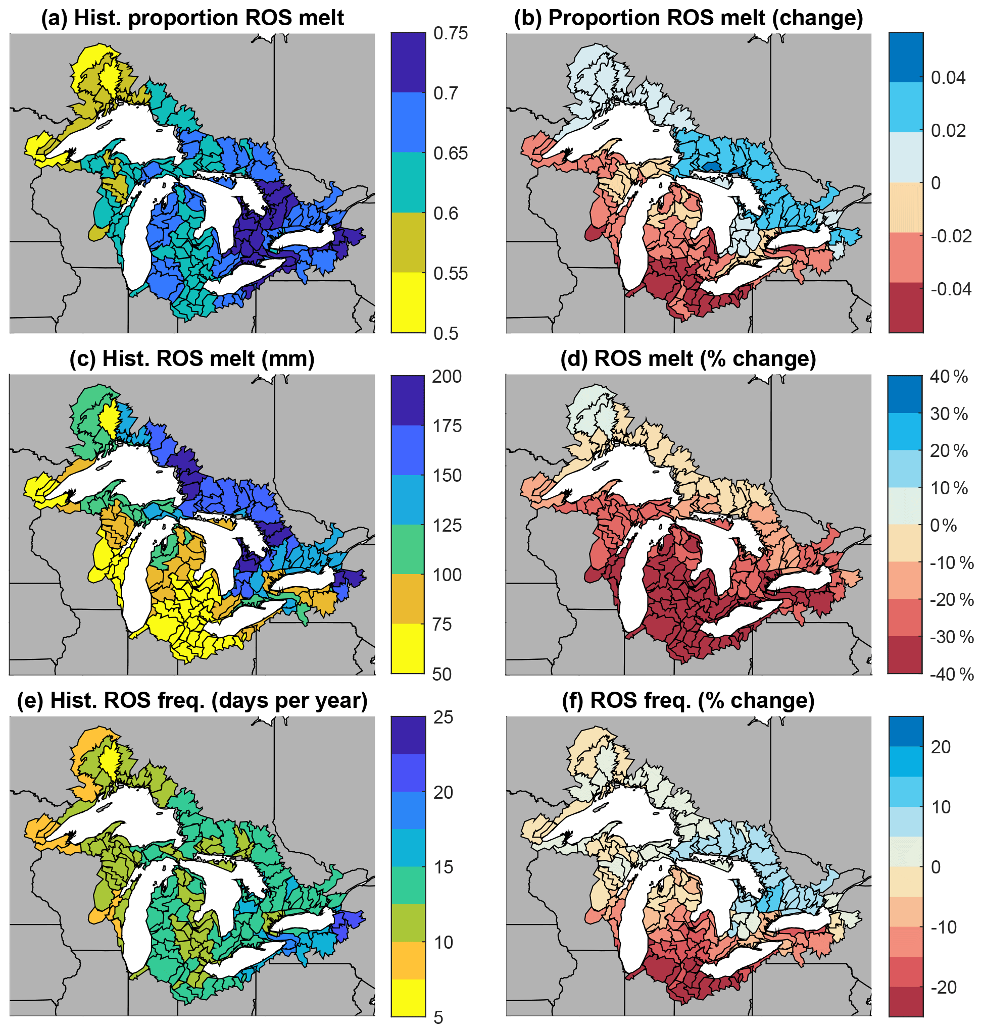
Figure 6 Changes in (a, b) the proportion of total snowmelt from ROS, (c, d) subbasin ROS melt, and (e, f) frequency of ROS events between the historic (1960–1999) period and mid-21st century. (a, c, e) Historic conditions. (b, d, f) Absolute or percent changes. Projections represent the RCP4.5 ensemble mean.

3.3 ROS melt projections

ROS melt is affected by the changing climate, and there will be different intensities and frequencies of ROS melt events in the future using the RCP4.5 pathway. The northernmost subbasins near Lake Superior experience the fewest changes in the annual amount of ROS melt between the historic (1960–1999) period and mid-21st century, with less than a 5 % change. However, the central and southern areas of the basin experience large decreases in annual ROS melt, with the greatest reduction in southern subbasins in Michigan and southern Ontario, with a >30 % decrease in the amount of annual ROS melt and a >20 % decrease in the frequency of ROS events (Fig. 6c–f). Overall, at the major river basin scale using the RCP4.5 scenario, the ensemble average amount of annual snowmelt during ROS events changes by −42 % to +1 %, with a basin-wide, area-weighted average of −22 % (p<0.001). Meanwhile, the range among climate projections in the ensemble for this change in the basin-wide average annual snowmelt during ROS events is −50 % to −3 %, suggesting that the climate models agree that there will be a reduction in annual ROS melt for the basin overall.

Additionally, northern and central subbasins around eastern Lake Huron and the southern shore of Lake Superior tend to see a slight increase in the annual frequency of ROS events of +5 %, while more southern subbasins experience the greatest decrease in frequency around −25 % (Fig. 6e and f). This is because the northern subbasins, which maintain substantial snowpack throughout the winter and spring and have temperatures well below freezing, have ROS frequencies that are resilient to increases in air temperature (through mid-century), while ROS frequencies in southern subbasins with combined winter and spring air temperatures around the freezing and melting points are sensitive to even small perturbations in air temperature, with threshold-like responses around these temperature points to the partitioning between rainfall and snowfall.

Following the earlier timing of ROS melt, the center of volume for ROS melt (the day of the water year when half of the total annual ROS melt is passed) decreases between the historic (1960–1999) period and mid-21st century. Historically, the ROS melt center of volume ranged from day 145 (23 February) in the southern part of the Great Lakes Basin to day 207 (26 April) in the northern part (Fig. 7a). By the mid-21st century, the ROS melt center of volume becomes earlier and ranges from day 134 (12 February) to day 198 (16 April), which is approximately 2 weeks earlier (Fig. 7b).

3.4 Relationships with climate and snowpack

The cause of the reduction in annual ROS melt across the basin is largely from a reduction in snowpack SWE due to the rising air temperatures. Although an increase in ensemble average combined winter and spring precipitation in major river basins by +7 % to +15 % contributes to ROS melt (Figs. 3a and 4c–f), its influence is negated by a decrease in the annual amount of winter snowpack SWE in river basins of −10 % to −52 % (Fig. 7c and d). This is due to proportionally more winter rainfall, as the combined winter and spring rain-to-snow ratio increases from 1.55±0.32 (mean and standard deviation of GCM ensemble) during the historic (1960–1999) period to 1.91±0.31 by the mid-21st century (Fig. 3c).

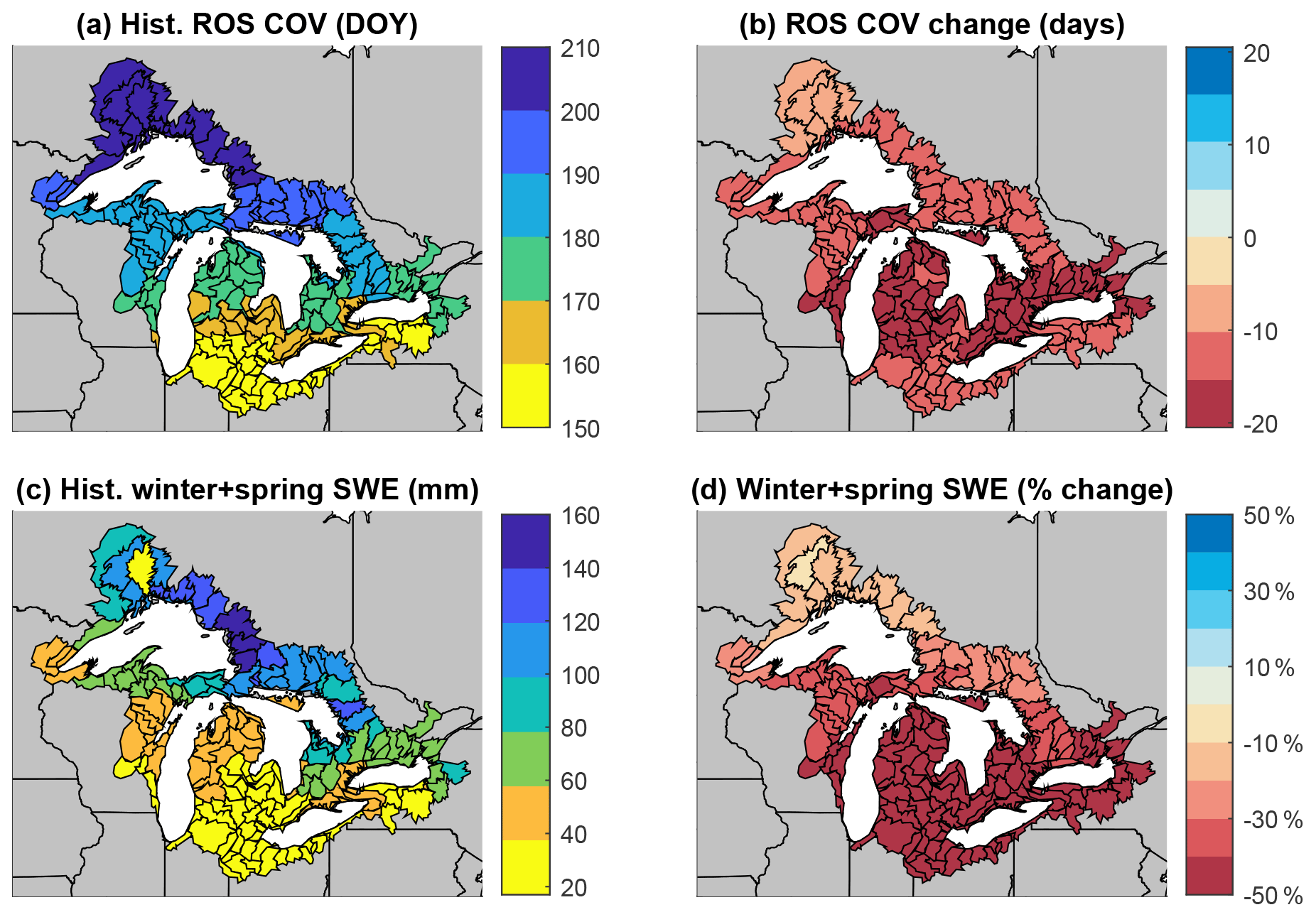
Figure 7 Changes in (a, b) the center of volume (COV) for ROS events (the day of the water year (DOY) when half the total annual ROS melt is passed) and (c, d) daily mean combined winter and spring snowpack SWE between the historic (1960–1999) period and mid-21st century. (a, c) Historic conditions. (b, d) Percent changes. Projections represent the RCP4.5 ensemble mean. The water year lasts from 1 October to 30 September.

Changes in the annual amount of ROS melt are strongly correlated with historic combined winter and spring snowpack SWE (r=0.87; p<0.001) and also with the frequency of ROS events (r=0.82; p<0.001). These relationships are also related to the location, with higher latitudes experiencing less of a change in ROS melt and frequency (Fig. 8a and b). A decrease in combined winter and spring SWE is consistently larger in the southern subbasins, where warming mean temperatures above the freezing and melting points reduce the ability of snow to accumulate (Fig. 7d). The lack of snowpack means that ROS melt events may be unable to occur as often or as intensely in these southern subbasins as they were able to historically. Changes to the amount of annual ROS melt and frequency of ROS events are not correlated with historic winter and spring total precipitation amounts (Fig. 8c and d), as the type of precipitation is more influential and depends on air temperatures (and thus latitude).

Figure 8 Relationships between the historic (1960–1999) conditions and the percent change from the historic period to mid-21st century for RCP4.5 ensemble means. (a) Historic combined winter and spring SWE and ROS melt amount change, (b) historic combined winter and spring SWE and ROS frequency change, (c) historic combined winter and spring precipitation and ROS melt change, (d) historic combined winter and spring precipitation and ROS frequency change, (e) historic combined winter and spring air temperature and ROS melt change, and (f) historic combined winter and spring air temperature and ROS frequency change. Colors are coded with the latitudinal gradient.

Mean historic winter and spring air temperatures have a strong relationship with changes to ROS melt. Subbasins that have colder combined winter and spring air temperatures during the historic (1960–1999) period have weaker changes to the amount of ROS melt ($r=-\mathrm{0.95}$; p<0.001; Fig. 8e) and frequency of ROS events ($r=-\mathrm{0.72}$; p<0.001; Fig. 8f). For example, subbasins in the Lake Superior watershed historically have mean combined winter and spring air temperatures of around −5 ^∘C (Fig. 4a). Even with an increase in mean combined winter and spring air temperatures of +3 ^∘C (Fig. 4b), temperatures remain cold enough to have a reduced influence on ROS occurrences for much of the winter and spring. Areas in which ROS is most sensitive to the changing climate are the central and southern river basins of the Great Lakes Basin, where historic mean combined winter and spring air temperatures were around 0 ^∘C. Here, perturbations to air temperatures due to climate change can have the greatest effects on ROS melt, leading to decreases in the amount of annual ROS melt stronger than −30 %, as the locations that experience these temperatures are often near the freezing and melting points (Fig. 6c and d).

3.5 Relationships with seasonal hydrology

The earlier center of volume for ROS melt has a lagged response on monthly water yields for the major river basins that lasts throughout the spring but becomes obscured by summer. There is a positive correlation between changes in the ROS melt center of volume and March (r=0.42; p<0.001) and April (r=0.70; p<0.001) water yields between the historic (1960–1999) period and mid-21st century, due to the influence of ROS melt on daily water yields when snowpacks are actively melting (Fig. 9a and b). In May, this relationship abruptly switches to negative ($r=-\mathrm{0.33}$; p<0.001), as the reduced impact of ROS means that less water is rapidly exported from the watershed during large melt events, and there is a delayed contribution to water yield (Fig. 9c). However, by the summer months of June, July, and August, correlations are weak, if any (Fig. 9d–f). Changes in summer water yields have much stronger relationships with summer precipitation than they do with ROS, for instance, in July (r=0.74; p<0.001) and August (r=0.84; p<0.001), obscuring the influence of the timing of ROS melt on summer water yields over time. This suggests that the earlier timing of ROS melt events (by center of volume) is related to hydrology through the spring, although the relationship can be obscured by summer by other factors such as summer precipitation.

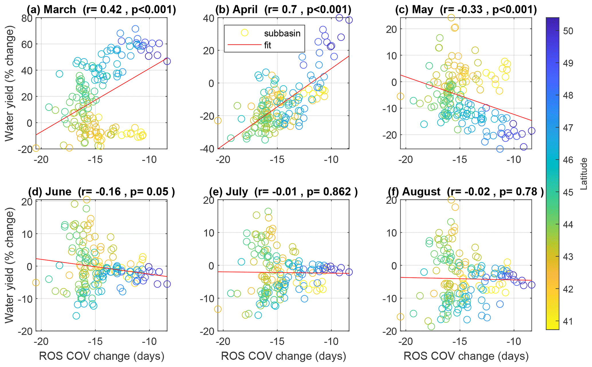
Figure 9 Correlations of the change in the COV for ROS melt events between the historic (1960–1999) period and mid-21st century, with the percent change in monthly water yield during that time for spring and summer months. Markers represent projections of the RCP4.5 ensemble mean for individual major river basins. Colors are coded with the latitudinal gradient. The water year lasts from 1 October to 30 September.

4 Discussion

4.1 Implications

It is important to understand the factors affecting spatial variability in ROS changes in the Great Lakes Basin to realize the impacts of this variability on aquatic resources. Spatial variability in ROS melt changes has previously been shown to occur because of differences in latitude, elevation, and atmospheric processes (Pan et al., 2018; Ye et al., 2008; Jeong and Sushama, 2018; Cohen et al., 2015), although there were not large elevation changes in the Great Lakes Basin to observe elevation-based variability at our scale. There are particularly large increases in ROS melt runoff predicted for northeastern North America but decreases in more southern latitudes due to a decrease in snow cover (Jeong and Sushama, 2018). The frequency of ROS melt events can be affected by latitude because of its association with air temperature, precipitation type (rain or snow), and snow cover (Suriano, 2022). This aligns with our findings for the Great Lakes Basin that the change in ROS melt amounts decreases by mid-century and is strongly related to latitude, with the greatest decreases in southern subbasins, where snowpack becomes exhausted, as latitude affects whether mean winter air temperatures will be near the threshold around the freezing and melting points, where ROS is most sensitive to changes in climate.

Similarly, an understanding of the temporal factors affecting variability in ROS changes can provide insights to the timing of hydrological impacts. Temporally, the frequency of ROS events in a warming climate has the potential to increase as more rain falls on snowpack but decline after a warming threshold is reached and the snowpack becomes scarce (Beniston and Stoffel, 2016). For instance, in eastern Russia, the frequency of ROS events has historically increased with warming air temperatures because of more winter rainfall, at a rate of 0.5 to 2.5 events per degree Celsius of air temperature increase, but future increases could be limited by a lack of snow in warmer regions (Ye et al., 2008). Suriano (2022) has found snowfall amounts to be a dominant control on the frequency of North American ROS melt events.

The earlier timing of ROS melt (and earlier passage of its annual center of volume) has the potential to influence other parts of the hydrologic cycle. In the eastern USA, since 1940, the timing of the center of streamflow volume passing through gages in the winter and spring has become earlier, at a rate of 1.6 d per decade, due to increasing air temperatures in snowmelt-driven regions and earlier snowmelt occurrences (Dudley et al., 2017). A similar trend of earlier snowmelt timing has been found for the western USA as well (Stewart et al., 2004; Musselman et al., 2021b). The earlier timing of snowmelt aligns with what our projections show for the basin overall, due to winter precipitation increases and ROS, supporting that the earlier center of volume for ROS melt could influence spring water yields. Also, following a 2 ^∘C warming scenario, prior research has found that the frequency of ROS melt events are expected to become approximately 1 month earlier in the eastern USA as cold-season snowfall switches to rainfall (Li et al., 2019), which aligns with our findings for the earlier center of volume for ROS melt over the water year. As the contributions of snowmelt to peak spring water yields become weaker due to the earlier timing of ROS events, vegetation green-up can have a more dominant influence on spring hydrographs in a changing climate (Khodaee et al., 2022).

Changing rain-to-snow ratios can have meaningful impacts on hydrological systems. The rain-to-snow ratio is important because it was previously found to be the primary avenue for changing air temperatures to affect snowpack in the Sierra Nevada of California, USA, exacerbating runoff during early season flooding (Huang et al., 2018). As more precipitation falls as rain rather than snow, the size of floods from rainfall and ROS events can far exceed the size of typical snowmelt-driven floods, due to the rapid contributions of rainfall and ROS runoff, with the largest increases being over 2.5 times in size for the western USA (Davenport et al., 2020). The rain-to-snow ratio can also influence the size and timing of spring snowmelt and summer baseflow (Huntington et al., 2004). Thus, the rain-to-snow ratio could help explain the earlier center of volume (COV) of ROS melt for the Great Lakes Basin by the mid-21st century, since we found that, as the basin-averaged rain-to-snow ratio increases from approximately 1.5 historically to 1.9 by mid-21st century, the COV of ROS melt occurs 2 weeks earlier.

The proportion of total snowmelt from ROS or temperature-based melt also has important hydrological impacts. Research in the western USA has found that climate change can decrease the speed at which snowpack melts, as warmer air temperatures mean that there will be bare ground later in the snowmelt season, while radiative energy fluxes are high, and more snowmelt occurs during the colder part of winter when energy fluxes are low, causing snowmelt to be a slower process (Musselman et al., 2017). This increase in the proportion of temperature-based melt to total snowmelt reflects a transition to slower, earlier snowmelt and helps explain the decrease in high spring streamflow that historically influenced hydrological regimes in the Great Lakes Basin (Hodgkins et al., 2007). The decrease in the proportion of total snowmelt from ROS in the Great Lakes Basin could also contribute to groundwater recharge (Earman et al., 2006; Wilson et al., 1980) and the increases in May water yields in subbasins where the annual amount of ROS decreases (Fig. 9c), as the water would not have been rapidly exported from the subbasins in earlier ROS events.

4.2 Historic ROS melt

Previous work by Jeong and Sushama (2018), whose definition of ROS we adopted, produced estimates of historic frequencies of ROS events comparable to ours, with approximately 10–20 ROS days per year in the Great Lakes Basin. Also, Jeong and Sushama (2018) report a 1976–2005 average annual amount of ROS runoff of approximately 100 mm or greater throughout the basin, which is similar to our historic (1960–1999) estimates that were approximately 75 mm annual ROS melt in the southwestern part of the basin and 175 mm in the northeast. Jeong and Sushama (2018) evaluated their model results using observations and found that spatial patterns in ROS were captured reasonably well, although some errors likely were due to data uncertainties rather than model errors. Using a different definition of a ROS event (air temperature > 0 ^∘C and precipitation > 5 mm during 2 d extreme snowmelt events), Welty and Zeng (2021) produced far fewer ROS events than we did. Additionally, Suriano (2022) defined a ROS event as a snow depth decrease of at least 1 cm, with average daily temperature > 0 ^∘C, at least 0.01 cm precipitation, and no more than 2.54 cm snowfall (by depth) on the previous day, over a historic (1960–2009) period. With this definition, Suriano (2022) reported a historic frequency of approximately 5 to 15 ROS events per year in the Great Lakes Basin, which is slightly less than our estimate of approximately 10–20 annual ROS events during 1960–1999.

To verify our historic estimates, we identified ROS amounts and frequencies in observed data using the same approach and definition as our GCM-forced SWAT model. The historic climate observations were from Maurer et al. (2007), used in Myers et al. (2021b), and our historic SWE observations were from Myers et al. (2021b), which had been estimated from the daily gridded North American snow depth dataset (Mote et al., 2018), both using the same 1^∘ latitude/longitude grid with 50 evaluation points over the Great Lakes Basin. We found that, for historic annual estimates of ROS melt, the mean among the gridded evaluation points for our GCM ensemble was 120 mm, while the mean calculated from observations was 118 mm, which was not a significant difference (two-sample t test; p=0.90). For individual evaluation points, the estimates of annual ROS melt were positively related and had a MAE of 33 mm (Fig. S1a in the Supplement). This suggests that our GCM ensemble produced reasonable estimates of historic ROS melt amounts in the basin. We also found that the historic observations produced an average annual ROS frequency of 20 d across the evaluation points, which was greater than the mean of 12 d estimated by our GCM ensemble for the points over the historic (1960–1999) period (p<0.001). This was because our ROS definition included historic observed events that were the result of natural stochasticity in snowpack SWE amounts (i.e., sporadic daily increases or decreases in the SWE data due to factors such as the timing of measurements at different stations, rather than clean modeled melt; Suriano and Leathers, 2017; Suriano, 2022). Thus, our definition underestimated the frequency of ROS days when applied to model data, due to the lack of additional stochastic small melt events identified by the criteria, producing a MAE of 8 d between observations and modeled ROS frequency (Fig. S1b). However, when ROS amounts are accumulated over the season, then this issue is remedied (Fig. S1a).

5 Conclusions

Climate change is disrupting ROS patterns globally, potentially impacting ecosystems, communities, and economies in regions where these events are prevalent. This study used the Soil and Water Assessment Tool (SWAT) rain-on-snow (ROS) melt model, which builds upon SWAT by incorporating energy budget equations to simulate ROS melt (Myers et al., 2021b), to study the impacts of climate change on ROS melt due to altered snowpack, air temperatures, and precipitation. An ensemble of RCP4.5 climate projections (representing moderate greenhouse gas concentrations) was used to study the relationships. Although combined winter and spring precipitation increases in the Great Lakes Basin by the mid-21st century, compared with historic (1960–1999) amounts, its influence on ROS melt is limited by an exhausted snowpack with warmer air temperatures, particularly for southern subbasins. Combined winter and spring rain-to-snow ratios from the climate input data rise from around 1.5 historically to 1.9 by mid-21st century, so proportionally more rainfall decreases snowpack SWE. Changes in ROS melt are positively correlated with snowpack snow water equivalent and combined winter and spring precipitation.

We find that relationships with ROS patterns and latitude are strong in the Great Lakes Basin, as ROS amounts in northern subbasins that had mean combined winter and spring air temperatures well below freezing are more resilient to air temperature increases, while southern subbasins that had mean combined winter and spring temperatures around freezing historically are more sensitive to changes in air temperature. The changing temperature directly affects whether snowpack would form or melt or whether precipitation would be snow or rain. We expect this result of increased sensitivity for ROS changes to apply to cold regions around the globe with average combined winter and spring air temperatures around 0 ^∘C. With increasing air temperatures, temperature-based snowmelt can have more of an influence on total monthly snowmelt, as the proportion of monthly melt from ROS decreases (e.g., −12 % in December) between the historic (1960–1999) period and mid-21st century.

We also find there are temporal relationships with ROS melt timing in the Great Lakes Basin by mid-21st century, as the center of volume (the day of the water year when at least half the total ROS melt volume has passed) becomes earlier by approximately 2 weeks when compared to the historic (1960–1999) period. The temporal scale of impacts from this earlier timing on monthly water yields lasts through the spring (positively correlated in March and April but negative in May), although these relationships can be obscured by summer because of changing summer precipitation. Investigations projecting the response of extreme water yields to changing ROS conditions in future climates are an additional avenue for future research, with meaningful implications for water resources management.

Finally, it is important that future work involve collaborations outside the academic realm so that the findings of climate change impacts to ROS melt can inform management of aquatic resources (Meadow and Owen, 2021) and engage communities with the research (Serreze et al., 2021). Future work could also investigate how changing ROS conditions affect other components of the water balance, including groundwater and soil water storage in the Great Lakes Basin. The implications of this work, specifically involving the influence of changing ROS melt on extreme hydrological events and future water availability, in addition to the climate-related sensitivities to changing ROS melt, could help prepare managers of ecosystems and human water use for the climatic changes in the mid-21st century.