A storm-centered multivariate modeling of extreme precipitation frequency based on atmospheric water balance

Conventional rainfall frequency analysis faces several limitations. These include difficulty incorporating relevant atmospheric variables beyond precipitation and limited ability to depict the frequency of rainfall over large areas that is relevant for flooding. This study proposes a storm-based model of extreme precipitation frequency based on the atmospheric water balance equation. We developed a storm tracking and regional characterization (STARCH) method to identify precipitation systems in space and time from hourly ERA5 precipitation fields over the contiguous United States from 1951 to 2020. Extreme “storm catalogs” were created by selecting annual maximum storms with specific areas and durations over a chosen region. The annual maximum storm precipitation was then modeled via multivariate distributions of atmospheric water balance components using vine copula models. We applied this approach to estimate precipitation average recurrence intervals for storm areas from 5000 to 100 000 km² and durations from 2 to 72 h in the Mississippi Basin and its five major subbasins. The estimated precipitation distributions show a good fit to the reference data from the original storm catalogs and are close to the estimates from conventional univariate GEV distributions. Our approach explicitly represents the contributions of water balance components in extreme precipitation. Of these, water vapor flux convergence is the main contributor, while precipitable water and a mass residual term can also be important, particularly for short durations and small storm footprints. We also found that ERA5 shows relatively good water balance closure for extreme storms, with a mass residual on average 10 % of precipitation. The approach can incorporate nonstationarities in water balance components and their dependence structures and can benefit from further advancements in reanalysis products and storm tracking techniques.

1 Introduction

The probability of extreme rainfall is of great interest and importance in flood risk estimation and management (e.g., Koutsoyiannis et al., 1998; Langousis et al., 2009; Nerantzaki and Papalexiou, 2022; Troutman and Karlinger, 2003). Standard practice is to fit a univariate probability distribution to either the largest rainfall observations each year (an annual maxima series) or the rainfall values that exceed a high threshold (a peaks-over-threshold or partial duration series (Coles, 2001; Madsen et al., 1997; Miniussi et al., 2020). In either case, the rainfall series corresponds to a given duration (e.g., 1, 24 h, etc.) and spatial scale. The latter is usually the sampling orifice of a rain gauge (roughly 0.1 m²), although larger spatial scales are within reach via techniques such as area reduction factors (ARF; e.g., Durrans et al., 2002), spatial interpolation (e.g., Yang et al., 2015), and stochastic storm transposition (Wright et al., 2013). The resulting probability distributions are then used to extrapolate tail quantiles such as the 100-year average recurrence interval (ARI) storm, which has a 0.01 annual exceedance probability. Though such approaches have proved extremely useful through decades of research and practice, they are not without limitations. To motivate this study, we highlight two such shortcomings here.

First, relying exclusively on rainfall observations – as opposed to using atmospheric and land surface processes and variables that contribute to rainfall – can preclude knowledge and measurements that could be informative for precipitation frequency analysis (Katz et al., 2002; Klemeš, 1993). This contrasts with techniques that estimate probable maximum precipitation – widely used in flood hazard analyses for major dams and nuclear facilities – which for decades have considered concepts and measurements of atmospheric water vapor storage and transport (e.g., Chen and Bradley, 2006; Rakhecha and Clark, 1999; Rousseau et al., 2014; World Meteorological Organization, 2009), and have recently expanded to dynamic atmospheric simulations (e.g., Alaya et al., 2018; Lee and Kim, 2018; Toride et al., 2019). To overcome this limitation, some recent rainfall frequency studies have attempted to use rainfall-related variables (e.g., sea surface temperature and dew point temperature) and changes in large-scale weather systems as predictors of rainfall frequency and its changes (see, e.g., Kunkel et al., 2020; Roderick et al., 2020a).

Second, while a single rain gauge can provide local observations that lead to ready-to-use quantile estimates (e.g., for flood hazard modeling), it severely restricts the number of extremes and cannot represent areal maxima over a large region. This is because much of the instrumental record at a gauge consists of local and smaller events, which have limited value for understanding rarer and more extreme storms at large scales (e.g., Durrans et al., 2002; Steiner et al., 1999; Svensson and Jones, 2010). While this shortcoming can be ameliorated using regionalization techniques that utilize multiple nearby gauges (e.g., Dawdy et al., 2012; Schaefer, 1990), these gauge-based analyses still struggle to represent precipitation areal maxima due to rain gauges' limited sampling area (Matsoukas et al., 1999; Villarini et al., 2008) and the complexity of storm spatiotemporal extents (Efstratiadis et al., 2014; Krajewski, 1987).

In this study, we present an alternative approach for rainfall frequency analysis that addresses these two aforementioned limitations. Here, we highlight two key features of our approach:

• First, our approach integrates a more physically detailed (albeit still highly simplified) rainfall-producing process. Specifically, we consider the atmospheric water balance equation, in which the change of water vapor storage within a control volume is balanced by water vapor flux in and out – namely precipitation, evapotranspiration, and water vapor flux convergence (Bradbury, 1957; Banacos and Schultz, 2005; Su and Smith, 2021). Due to mass conservation, precipitation can be modeled as a combination of the remaining components that jointly form a multivariate distribution (Alaya et al., 2020; Klemeš, 1993; Gao et al., 2005). Previous multivariate precipitation modeling of precipitation frequency can be seen in De Michele and Salvadori (2003), Jun et al. (2017), and Salvadori and De Michele (2007), but these focused on joint modeling of “precipitation dimensions” (e.g., rainfall intensity, volume, and duration) rather than the atmospheric water balance. Here, we use vine copulas to represent this multivariate distribution by decomposing it into bivariate dependence structures and marginal distributions (Aas et al., 2009). Applications of vine copula models have been seen in risk analysis (Bevacqua et al., 2017; Sarhadi et al., 2018; Xiong et al., 2014), rainfall simulation (Gyasi-Agyei and Melching, 2012; Vernieuwe et al., 2015), and streamflow modeling (Pereira and Veiga, 2018), but to the best of our knowledge, no study has applied vine copulas to extreme rainfall frequency analysis.

• Second, our approach is “storm-centered” (Chang et al., 2016; Li et al., 2020; National Research Council, 1988, 1994) rather than gauge-centered. We use storm tracking methods to identify and follow two-dimensional rainfall systems (i.e., storm objects) in space and time within a land–atmosphere reanalysis dataset. These storm objects, particularly their high-rainfall areas, are considered as control volumes to compute the atmospheric water balance for multivariate modeling. Our “storm-centered” approach has three main properties: (1) unlike gauge-centered approaches (Restrepo-Posada and Eagleson, 1982), we can identify all major storms over a region. (2) We can examine precipitation frequency and drivers over user-defined areas, rather than over the spatial scale of a rain gauge orifice. This further allows us to derive “storm-centered” depth–area–duration (DAD) relationships and ARIs over a region. Specifically, based on areal precipitation extracted from storm objects, we can characterize how precipitation estimates change with storm area, given a certain ARI and storm duration. (3) The ARIs estimated by our approach represent the frequency of extreme storms within a chosen region. Such ARIs should be interpreted differently from those in traditional gauge-based analysis that represent local precipitation frequencies. The last two properties are discussed in more detail in Sect. 5. Previous “storm-centered” studies have investigated precipitation properties based on observations and model simulations (e.g., Chang et al., 2016; Davis et al., 2006; Hoskins and Hodges, 2002; Pérez-Alarcón et al., 2022; Shaw et al., 2016). Though there has been long-standing recognition that storm-centered methods hold some advantages over gauge-based methods in rainfall frequency analysis (e.g., National Research Council, 1994), far fewer studies have explored the topic (see Wright et al., 2020 for recent review and discussion).

Table 1 Descriptions of used ERA5 variables.

The objective of this study is to develop an alternative approach for extreme precipitation frequency, by integrating storm tracking with a multivariate vine copulas model of atmospheric water balance. The approach allows an explicit representation of the dependencies between rainfall-contributing components. It also highlights some of the strengths and limitations of using reanalysis and other atmospheric simulations to study extreme rainfall and its drivers. We use the approach to investigate the frequencies and characteristics of major storms in the Mississippi Basin and its five major subbasins. The remainder of the paper is organized as follows: Sect. 2 describes the study basin and datasets. Section 3 details the proposed methods for storm identification and multivariate modeling. Results are shown in Sect. 4, followed by discussion in Sect. 5. Conclusions are provided in Sect. 6.

2 Study site and datasets

2.1 Study site

The study site is the Mississippi River Basin, located in the central United States with a drainage area of over 3 220 000 km² and consisting of five major subbasins: the Arkansas-Red, Missouri, Upper Mississippi, Ohio-Tennessee, and Lower Mississippi (Fig. 1). With abundant atmospheric moisture supply from the Gulf of Mexico and the Pacific (e.g., Benedict et al., 2020; Smith and Baeck, 2015), the Mississippi Basin has experienced multiple major storm-induced flood events in recent decades, including in 1993, 2011, and 2019 (Allison et al., 2013; Pal et al., 2020; Rabalais et al., 1998). These caused major socio-economic impacts throughout the basin (Mutel, 2010; Myers and White, 1993). Previous studies have shown links between extreme storms and anomalously large atmospheric water vapor transport (Holman and Vavrus, 2012; Su and Smith, 2021; Sudradjat et al., 2003) and high precipitable water (Kim et al., 2022; Kunkel et al., 2020b) in the basin.

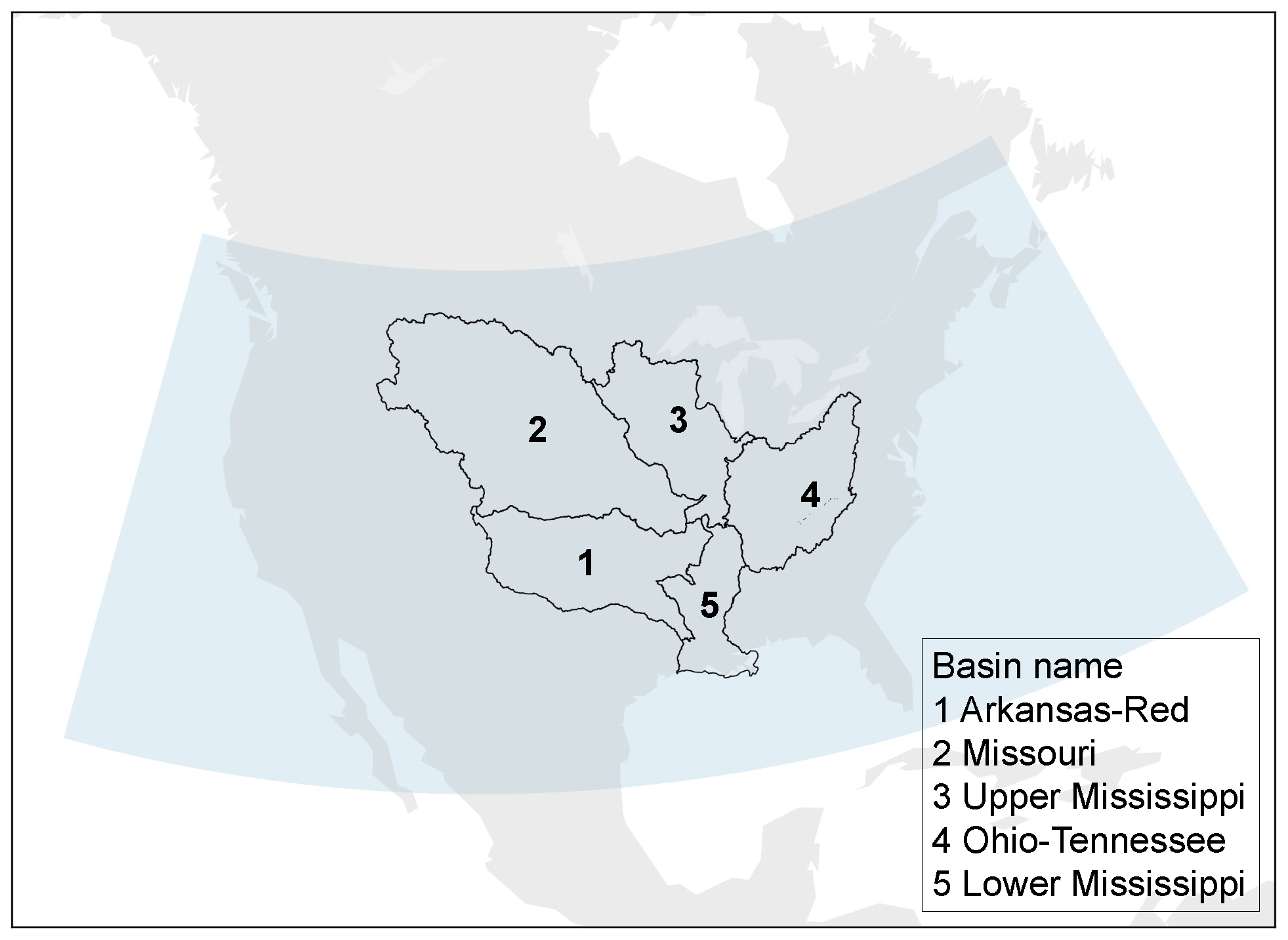
Figure 1 Mississippi Basin, including (1) Arkansas-Red, (2) Missouri, (3) Upper Mississippi, (4) Ohio-Tennessee, and (5) Lower Mississippi subbasins. Blue shading denotes the domain over which storm tracking was applied (24–52^∘ N, 60–130^∘ W).

2.2 Datasets

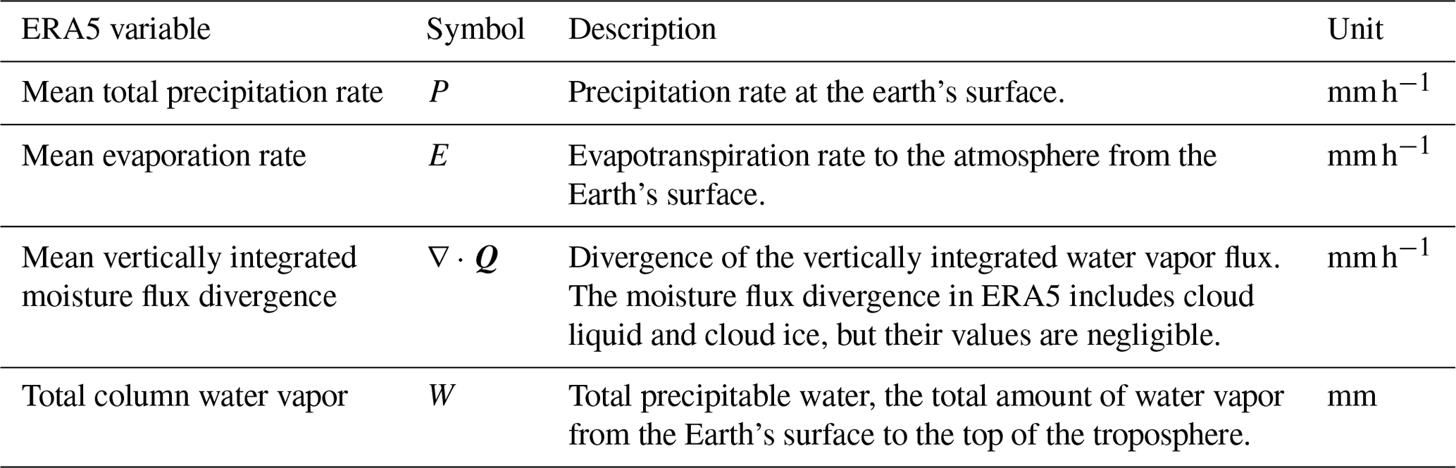
ERA5 Reanalysis was used to identify storms and to compute atmospheric moisture components. This dataset, produced by the European Center for Medium-Range Weather Forecasting (ECMWF), provides hourly estimates of global climate variables on a 0.25^∘ grid from 1950 to the present (Hersbach et al., 2020). Studies have shown that ERA5 has improved performance over its predecessor ERA-Interim due to advances in numerical schemes, data assimilation systems, and spatiotemporal resolution (Beck et al., 2019; Urraca et al., 2018; Zhang et al., 2018). In this study, we used 70 years of ERA5 hourly data from 1951 to 2020 over the contiguous United States (24–52^∘ N, 60–130^∘ W). The names and descriptions of the variables used are shown in Table 1.

Meanwhile, Integrated Multi-satellite Retrievals for Global precipitation measurement (IMERG) data from 2001 to 2019 were used to validate storm tracking results. IMERG surface precipitation rates are estimated globally on a 30 min 0.1^∘ scale using a constellation of satellite-based passive microwave and infrared sensors (Huffman et al., 2019); the Final Run version of IMERG V06B used here incorporates monthly gauge-based bias correction. We aggregated IMERG to the hourly scale and used a conservative method from the Python package “xESMF” (Zhuang et al., 2020) to regrid IMERG to 0.25^∘ grid to match the boundary and spatial resolution of ERA5.

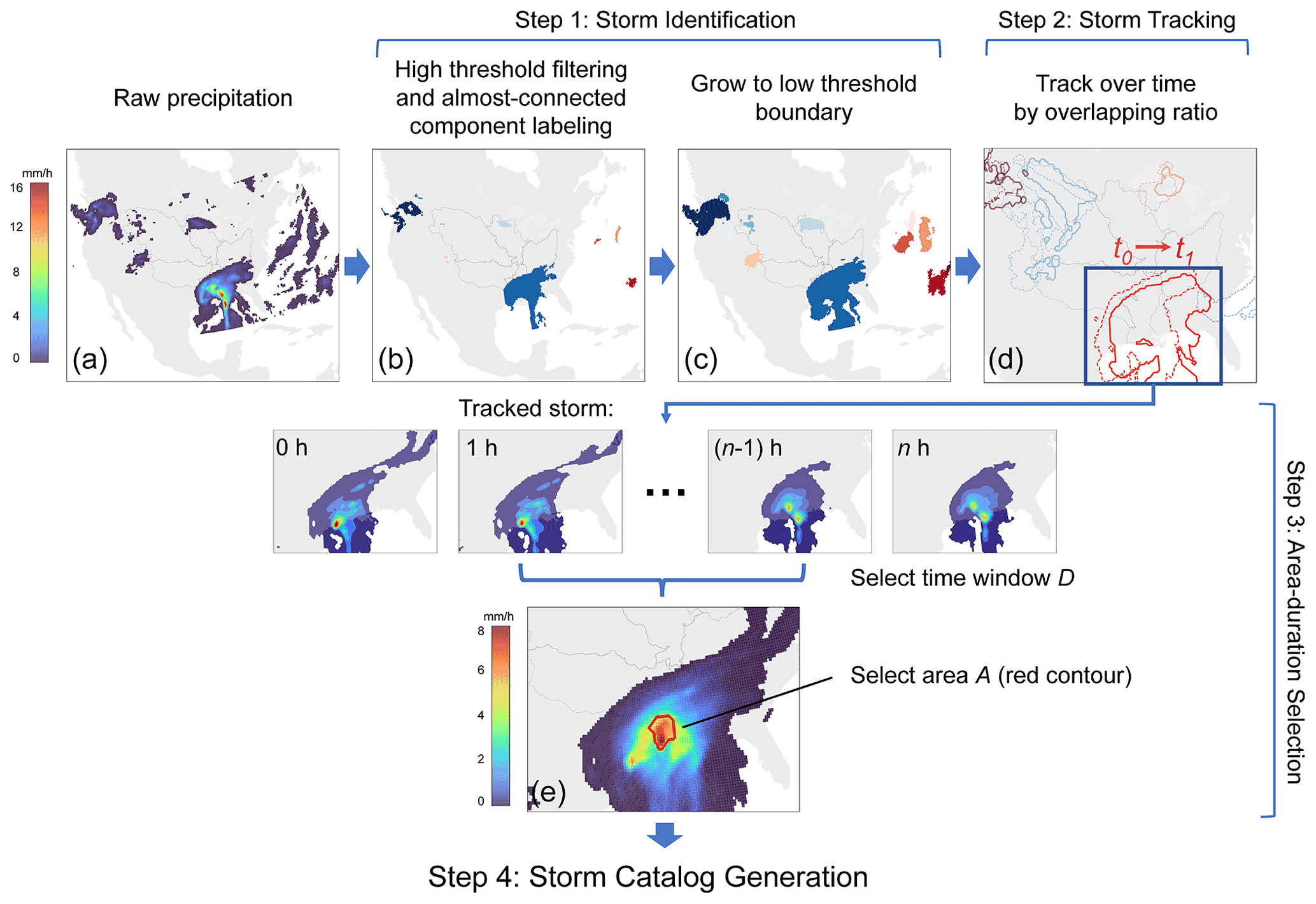
Figure 2 Process of the storm tracking and regional characterization method (STARCH). (a) ERA5 precipitation at 11:00 UTC on 25 October 2015; (b) identified storms after high threshold filtering (0.5 mm h⁻¹) and almost-connected component labeling; each color denotes one storm object; (c) identified storms after growing to low threshold boundaries (0.03 mm h⁻¹); (d) example of storm tracking. Dashed (solid) lines denote storm locations at 10:00 (11:00) UTC on 25 October 2015; (e) selected storm object (red) with 50 000 km² area and 24 h duration (11:00 UTC on 25 October to 10:00 UTC on 26 October 2015). Background colors denote the total precipitation in the 24 h period.

3 Methodology

3.1 Storm tracking and regional characterization method (STARCH)

To identify and analyze regional extreme storm events in the Mississippi Basin we developed the storm tracking and regional characterization method (STARCH, publicly available at https://github.com/lorenliu13/starch, last access: 18 September 2022). The method is a novel combination of two prior storm tracking algorithms: (1) double-threshold identification from the Thunderstorm Identification, Tracking, Analysis, and Nowcasting (TITAN) algorithm (Dixon and Wiener, 1993) and (2) “almost-connected component labeling” from the Storm Tracking and Evaluation Protocol (STEP; Chang et al., 2016). An area–duration selection algorithm is also developed to search storms with user-defined duration and area. STARCH can not only track storms based on successive two-dimensional precipitation fields but can also create catalogs of extreme storm events with specific areas and durations within a chosen region. The method, summarized graphically in Fig. 2, consists of four key steps:

• Step 1 – storm identification: individual storm objects within a precipitation field were identified at a single time step. First, an initial threshold of 0.5 mm h⁻¹ was applied to the precipitation field to identify storm regions. Second, almost-connected-component labeling classified closely distributed precipitating regions as a single storm (Fig. 2b). This labeling algorithm used a circular morphing structure with radius R_m to erode and dilate precipitating regions, clustering small regions with nearby larger ones (more details on almost-connected labeling can be found in Chang et al., 2016). Lastly, the identified storm objects were morphologically “grown” to a low threshold boundary of 0.03 mm h⁻¹ (Fig. 2c). The combination of two thresholds with the almost-connected component labeling algorithm can accurately identify individual storms while preserving original storm structures. Since a storm system can consist of multiple separated precipitation regions, using a single threshold usually results in either too many isolated objects or too few overly-large storms (Steiner et al., 1995). A high threshold within the labeling algorithm can help associate high-precipitation storm centers with nearby low-precipitation areas. After that, growing to a low boundary preserves more precipitation grids and can thus better represent the original storm spatial structures. The high and low thresholds were chosen through visual inspection and trial and error.

• Step 2 – storm tracking: in this step, storms were tracked across time steps using the overlapping ratio method (NCAR, 2019). For storm i in current time step t₁ and storm j in previous time step t₀, the overlapping ratio R is the sum of the proportions of the overlapping area to the two storm areas:

  $$\begin{array}{}\text{(1)}& R\left(t_{\mathrm{1}},i,j\right)={\displaystyle \frac{A}{A_i\left(t_{\mathrm{1}}\right)}}+{\displaystyle \frac{A}{A_j\left(t_{\mathrm{0}}\right)}},\end{array}$$

  where $R(t_{\mathrm{1}},i,j)\subset [\mathrm{0},\mathrm{2}]$ is the overlapping ratio, A is the overlapping area between storm i and storm j, A_i(t₁) is the area of storm i at time step t₁, and A_j(t₀) is the area of storm j at time step t₀; all the areas are measured by pixels. If two storm objects from Step 1 have a sufficiently high threshold value of R, they are deemed to be a single storm and tracked as such; otherwise, the more recent object is labeled as a new storm. If multiple possible matches are found between current storms and the previous storm, the two having the highest R are tracked. Based on visual inspection, two consecutive storm objects should generally have R>0.3, whereas two unrelated objects should have a value around 0. We selected an R threshold of 0.3 based on visual inspection and trial and error. An example of storm tracking is shown in Fig. 2d.

• Step 3 – area–duration selection: the third step is to extract extreme precipitation events of desired duration D and area A for each subbasin based on the storms identified in Steps 1 and 2. A storm was deemed to have occurred in a subbasin if its area within that subbasin exceeds 2500 km² (about 5 ERA5 pixels) or its average precipitation over the subbasin exceeded 0.1 mm h⁻¹. For such a storm in the subbasin, we extracted the D-hour period during which the storm had the highest total precipitation over the subbasin. Within that extracted period, we applied an area selection algorithm to find a contiguous region of area A that has the highest precipitation in the subbasin. To do this, a binary search was implemented to find a precipitation threshold whose corresponding contour area on the total precipitation map is close to but less than the desired area A. We began with a threshold at the midrange of the precipitation interval, i.e., (maximum + minimum)$/\mathrm{2}$ and computed the contour areas, i.e., areas of precipitation regions above the threshold. The largest contour area was compared with the desired area A. If the contour area was less than A, we narrowed the precipitation interval to the lower half, i.e., from the minimum to the midrange. Otherwise, we narrowed the interval to the upper half. We then repeatedly calculated the midrange of the new interval as the next threshold and compared the contour area with the desired area A. All the thresholds and associated contour areas were recorded throughout the iterations. The binary search stops if the difference between the contour area and desired area is less than one pixel, or the selected contour area does not change in three consecutive iterations. From the search record, we found a threshold with a contour area that is close to but less than the desired area A. Thereafter, the area selection algorithm recursively expands and recalculates the contour by one pixel at a time until the difference between the contour area and area A is less than one pixel. An example of the area–duration selection result of a storm event of 24 h and 50 000 km² in the Lower Mississippi Basin is shown in Fig. 2e.

• Step 4 – storm catalog generation: the final step is to quantify storm characteristics and build annual maximum “storm catalogs”. For each storm selected in Step 3, we computed the storm area, duration, centroid speed, bearing (clockwise direction for north of centroid movement), and atmospheric water balance components (described below in Sect. 3.2). The annual maximum storm catalogs were created by collecting the largest storm each year with area A and duration D for the Mississippi Basin and each subbasin.

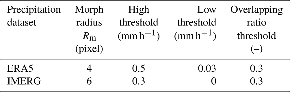
STARCH was applied to ERA5 from 1951 to 2020 and IMERG from 2001 to 2019 using the parameters from Table 2. Since the precipitation patterns in IMERG are somewhat more scattered than those in ERA5, we increased the morphing structure radius and reduced the precipitation thresholds to avoid overly isolated storm regions. The same overlapping ratio threshold was used for both datasets. Afterward, the area–duration selection was applied to ERA5 storms for the five subbasins and the whole Mississippi Basin. Values of storm area A were 5000, 25 000, 50 000, and 100 000 km², and values of storm duration D were 2, 6, 12, 24, 48, and 72 h. This combination of areas and durations resulted in 24 annual maximum storm catalogs for each subbasin and 144 cases in total.

Table 2 Parameter settings used in STARCH.

3.2 Atmospheric water balance

This study treats each storm area identified by STARCH as a control volume for computing a vertically integrated atmospheric water balance (Su and Smith, 2021), which can be written as

$$\begin{array}{}\text{(2)}& {\displaystyle \frac{\partial W}{\partial t}}=E-P-\mathrm{\nabla }\cdot \mathit{Q},\end{array}$$

where W is total precipitable water (mm), E is evapotranspiration to the atmosphere from the Earth's surface (mm h⁻¹, positive if directed upward, i.e., entering the storm control volume), P is precipitation (mm h⁻¹, positive if directed downward); ∇⋅Q is the divergence of the vertically integrated water vapor flux vector (mm h⁻¹, negative ∇⋅Q indicates convergence of water vapor into the storm). Equation (2) relates the temporal change in precipitable water to land surface evapotranspiration, precipitation from the atmosphere, and water vapor flux convergence; W, in units of mm, is defined as

$$\begin{array}{}\text{(3)}& W=\underset{\mathrm{0}}{\overset{z_t}{\int }}{\mathit{\rho }}_{\mathrm{v}}\left(z\right)\mathrm{d}z,\end{array}$$

where ρ_v(z) is the water vapor density (kg m⁻³), and z_t is the height of the troposphere above ground level. The divergence term is based on the vertically integrated water vapor flux vector $\mathit{Q}=(Q_x,Q_y)$, defined as

$$\begin{array}{}\text{(4)}& {\displaystyle }& {\displaystyle }{Q}_x=\underset{\mathrm{0}}{\overset{z_t}{\int }}{\mathit{\rho }}_{\mathrm{v}}\left(z\right)u\left(z\right)\mathrm{d}z,\text{(5)}& {\displaystyle }& {\displaystyle }{Q}_y=\underset{\mathrm{0}}{\overset{z_t}{\int }}{\mathit{\rho }}_{\mathrm{v}}\left(z\right)v\left(z\right)\mathrm{d}z,\end{array}$$

where u(z) and v(z) are the east–west and north–south components of the wind (m s⁻¹), Q_x and Q_y have the units of kg m⁻¹ s⁻¹, representing the mass flux of water vapor across a plane of unit width in the east–west and north–south directions, respectively, extending to the top of the troposphere.

All water balance components $\left(\frac{\partial W}{\partial t}\right.$, E, P, and ∇⋅Q) in Eq. (2) were computed for storms in each storm catalog described in Sect. 3.1 based on the ERA5 variables in Table 1. The time derivative term $\frac{\partial W}{\partial t}$ was computed by central differencing the total precipitable water W within the storm duration. These components form the basis of the multivariate extreme precipitation modeling described next.

3.3 Multivariate vine copula model

This section describes a multivariate vine copula model to estimate the frequency of extreme precipitation based on other atmospheric water balance components. According to Eq. (2), precipitation can be calculated as the sum of the evapotranspiration, water vapor flux divergence, and the time derivative of total precipitable water. In principle, the water balance is closed by mass conservation. However, due to data assimilation and differencing schemes, ERA5 does not guarantee water balance closure (see Sect. 5.1 for further discussion). Therefore, a residual error term was introduced to Eq. (2):

$$\begin{array}{}\text{(6)}& P=E-\mathrm{\nabla }\cdot \mathit{Q}-{\displaystyle \frac{\partial W}{\partial t}}+\mathit{\epsilon },\end{array}$$

where ε is the water balance residual (mm h⁻¹), i.e., the difference between precipitation and the sum of remaining water balance components.

Treating the right-hand side terms in Eq. (6) as random variables, precipitation can be represented by a multivariate distribution $P=F\left(E,\mathrm{\nabla }\cdot \mathit{Q},\frac{\partial W}{\partial t},\mathit{\epsilon }\right)$. According to Sklar's theorem, a four-variate distribution can be expressed using copulas and marginal distributions of random variables (Aas et al., 2009):

$$\begin{array}{}\text{(7)}& F\left(x_{\mathrm{1}},x_{\mathrm{2}},x_{\mathrm{3}},x_{\mathrm{4}}\right)=C\left(F_{\mathrm{1}}\left(x_{\mathrm{1}}\right),F_{\mathrm{2}}\left(x_{\mathrm{2}}\right),F_{\mathrm{3}}\left(x_{\mathrm{3}}\right),F_{\mathrm{4}}\left(x_{\mathrm{4}}\right)\right),\end{array}$$

where F(⋅) is the joint cumulative distribution function (CDF), F₁(x₁) ⋯ F₄(x₄) represent the marginal CDFs of the components on the right-hand side of Eq. (6), and C is the copula describing the dependence structure between those components. The joint probability density function (PDF) of the multivariate model p(⋅) can be factorized with conditioning:

$$\begin{array}{}\text{(8)}& \begin{array}{rl}p\left(x_{\mathrm{1}},x_{\mathrm{2}},x_{\mathrm{3}},x_{\mathrm{4}}\right)=& p\left(x_{\mathrm{1}}\mathrm{|}{x}_{\mathrm{2}},x_{\mathrm{3}},x_{\mathrm{4}}\right)p\left(x_{\mathrm{3}}\mathrm{|}{x}_{\mathrm{2}},x_{\mathrm{4}}\right)\\ & p\left(x_{\mathrm{2}}\mathrm{|}{x}_{\mathrm{4}}\right)p\left(x_{\mathrm{4}}\right),\end{array}\end{array}$$

among which the conditional PDF can be rewritten with a bivariate copula, for example:

$$\begin{array}{}\text{(9)}& \begin{array}{rl}p\left(x_{\mathrm{1}},x_{\mathrm{2}}\mathrm{|}{x}_j\right)=& c_{\mathrm{12}\mathrm{|}j}\left(F_{\mathrm{1}\mathrm{|}j}\left(x_{\mathrm{1}}\mathrm{|}{x}_j\right),F_{\mathrm{2}\mathrm{|}j}\left(x_{\mathrm{2}}\mathrm{|}{x}_j\right)\right)\\ & p\left(x_{\mathrm{1}}\mathrm{|}{x}_j\right)p\left(x_{\mathrm{2}}\mathrm{|}{x}_j\right),\end{array}\end{array}$$

where c_12|j is the copula density between x₁|x_j and x₂|x_j. Based on Eq. (9), Eq. (8) is further decomposed into bivariate copulas and marginal PDFs:

$$\begin{array}{}\text{(10)}& \begin{array}{rl}p\left(x_{\mathrm{1}},x_{\mathrm{2}},x_{\mathrm{3}},x_{\mathrm{4}}\right)& =p_{\mathrm{1}}\left(x_{\mathrm{1}}\right)p_{\mathrm{2}}\left(x_{\mathrm{2}}\right)p_{\mathrm{3}}\left(x_{\mathrm{3}}\right)p_{\mathrm{4}}\left(x_{\mathrm{4}}\right)\\ & \cdot c_{\mathrm{12}}\left(x_{\mathrm{1}}{x}_{\mathrm{2}}\right)c_{\mathrm{24}}\left(x_{\mathrm{2}},x_{\mathrm{4}}\right)c_{\mathrm{43}}\left(x_{\mathrm{4}},x_{\mathrm{3}}\right)T_{\mathrm{1}}\\ & \cdot c_{\mathrm{14}\mathrm{|}\mathrm{2}}\left(x_{\mathrm{1}\mathrm{|}\mathrm{2}},x_{\mathrm{4}\mathrm{|}\mathrm{2}}\right)c_{\mathrm{23}\mathrm{|}\mathrm{4}}\left(x_{\mathrm{2}\mathrm{|}\mathrm{4}},x_{\mathrm{3}\mathrm{|}\mathrm{4}}\right)T_{\mathrm{2}}\\ & \cdot c_{\mathrm{13}\mathrm{|}\mathrm{24}}\left(x_{\mathrm{1}\mathrm{|}\mathrm{24}},x_{\mathrm{3}\mathrm{|}\mathrm{24}}\right)T_{\mathrm{3}}.\end{array}\end{array}$$

The decomposition can be illustrated by the tree structure in Fig. 3a, where the nodes are variables and the edges are bivariate copulas; T₁, T₂, and T₃ are the tree levels that represent the corresponding parts of Eq. (10). This representation of the joint PDF via bivariate copulas is called a vine copula. Vine copulas hold advantages for high-dimension modeling, since one only needs to estimate bivariate copulas and corresponding conditional CDFs to obtain an estimator of the joint PDF. On the other hand, the decomposition in Eq. (8) is not unique, leading to different possible tree structures and necessitating model selection.

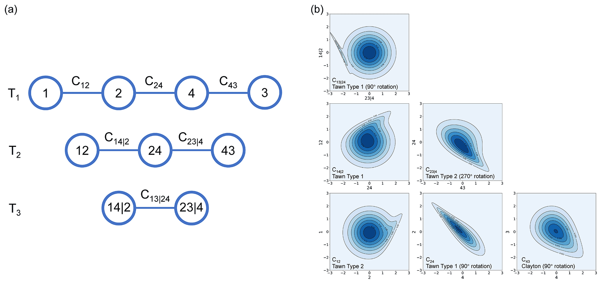
Figure 3 (a) A vine copula tree structure for atmospheric water balance components (d=4), where 1, 2, 3, and 4 represent water balance components. Note that the permutation is not unique and depends on model fitting; (b) normalized bivariate copula contour plots of all pair copulas specified in the copula tree structure in (a). The contour colors represent the copula densities.

We used the R package “VineCopula” to sequentially select vine structures and estimate copula parameters (Nagler et al., 2021). First, the tree structure at the top level (T₁) was determined by the max spanning trees to maximize the sum of the edge weights. The commonly used edge weight is the absolute value of Kendall's τ correlation coefficient between variables on the nodes. Second, for each pair of variables, the parameters of the bivariate copulas were estimated using maximum likelihood estimation, and the best bivariate copula was chosen based on the Akaike information criterion. The above procedure was repeated on the next tree level until reaching the bottom level to complete the vine copula estimation. The marginal CDFs of the water balance components are also required. We fitted empirical CDFs for E, $\frac{\partial W}{\partial t}$, and ε with Weibull plotting position (Dingman, 2015), which is commonly chosen in fitting vine copulas. However, empirical CDFs will constrain the simulated water balance components to the maximum in the sample data, which can lead to unrealistic upper-bounded tail behavior. To overcome this, we fitted the divergence term ∇⋅Q using the generalized extreme value (GEV; e.g., Walshaw, 2013) distribution:

$$\begin{array}{}\text{(11)}& F(x;\mathit{\mu },\mathit{\sigma },\mathit{\gamma })=\exp \left\{-{\left[\mathrm{1}+\mathit{\gamma }\left({\displaystyle \frac{x-\mathit{\mu }}{\mathit{\sigma }}}\right)\right]}^{-\frac{\mathrm{1}}{\mathit{\gamma }}}\right\},\end{array}$$

where F(⋅) is the CDF of the GEV distribution, x is the divergence term, $\mathit{\mu }\in (-\mathrm{\infty },+\mathrm{\infty })$ is the location parameter measuring the central tendency of extremes, $\mathit{\sigma }\in (\mathrm{0},+\mathrm{\infty })$ is the scale parameter measuring the variability of extremes; $\mathit{\gamma }\in (-\mathrm{\infty },+\mathrm{\infty })$ is the shape parameter that determines the type of the GEV distribution and tail behavior. We chose the divergence term to fit the GEV distribution because of its dominant role in the atmospheric water balance in extreme storms (described further in Sect. 4.4.2). The GEV distribution was estimated by the L moments method (e.g., Gubareva and Gartsman, 2010) via the R package “extRemes” (Gilleland and Katz, 2016). Figure 3b shows an example of a fitted vine copula model, where each subplot is a normalized bivariate copula contour representing the dependence structure between variables in Fig. 3a. The orientation of the contours denotes positive or negative tail dependence, while the contour width denotes the strength of the correlation.

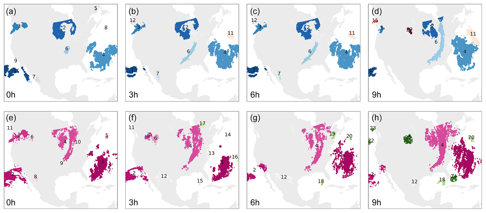
Figure 4 Comparison of storm tracking results based on ERA5 (a–d) and IMERG (e–h) starting at 20:00 UTC on 12 October 2015. Each tracked storm object is marked with one label and color through time.

For each annual maximum storm catalog described in Sect. 3.1 (144 cases in total), we fitted an individual vine model to the water balance components (E, ∇⋅Q, $\frac{\partial W}{\partial t}$, and ε). The fitted model was used to simulate samples, where each sample represents a possible combination of water balance components in an annual maximum event. “Synthetic” precipitation annual maxima were then calculated from these components based on Eq. (6). Model uncertainty was quantified via the parametric bootstrapping method of Bevacqua et al. (2017) and summarized here. First, a vine copula model was fitted based on the annual maximum storm catalog (n=70). Second, we used the fitted model to simulate samples of size 70 and repeated 100 times (i.e., to obtain 100 bootstrap realizations). Based on each bootstrap realization, we fitted a new vine copula model, retaining the same vine copula structure as that fitted based on the original storm catalog but reselecting and re-estimating the bivariate copulas. We used each fitted model to simulate 500 samples to calculate associated precipitation, equivalent to 500 years of annual maxima. Precipitation frequency was then estimated by the empirical CDF using the Cunnane plotting position (Cunnane, 1978; other plotting position formulae were tested and results were very similar):

$$\begin{array}{}\text{(12)}& \widehat{F}\left(x_{\left(i\right)}\right)={\displaystyle \frac{i-\mathrm{0.4}}{n+\mathrm{0.2}}},\end{array}$$

where $\widehat{F}(\cdot )$ is the empirical CDF, x_(i) is the ith ranked value of precipitation, and n is the number of simulated events. Another way of bootstrapping is to generate bootstrap realizations (n=70) by randomly sampling data with replacements from the annual maximum storm catalog and to use each realization to fit a vine copula model. These bootstrapping results were not shown because the estimates were similar.

We also computed relative root mean square error (RRMSE) to measure discrepancies between simulated and reference precipitation at the same recurrence intervals:

$$\begin{array}{}\text{(13)}& \mathrm{RRMSE}={\displaystyle \frac{\sqrt{\frac{\mathrm{1}}{n}\sum _{i=\mathrm{1}}^n{\left(x_{\left(i\right)}-x_{\left(i\right)}^{\mathrm{ref}}\right)}^{\mathrm{2}}}}{\frac{\mathrm{1}}{n}\sum _{i=\mathrm{1}}^n{x}_{\left(i\right)}^{\mathrm{ref}}}},\end{array}$$

where $x_{\left(i\right)}^{\mathrm{ref}}$ is the ith ranked reference precipitation from the storm catalog with recurrence interval empirically determined by the Cunnane plotting position, x_(i) is the ith mean simulated precipitation with the same recurrence interval, and n=70 is the size of the storm catalog.

4 Results

4.1 Storm identification and tracking

In this section, STARCH storm tracking results based on ERA5 were compared with those from IMERG. This comparison is intended to validate the basic spatiotemporal properties of ERA5-simulated storm systems against observation-based IMERG results. This was done via visual inspection of storm tracks and comparing storm characteristics between the two datasets for the 2001–2019 period. An example over 9 h is shown in Fig. 4. Precipitation regions in ERA5 are generally more contiguous in space than in IMERG. Despite some local differences, storm patterns are generally similar between the two datasets. This is confirmed by the large-sample comparison of the storm characteristics shown in Table 3. The average area (maximum precipitation intensity) of ERA5 storms is 7 % (2 %) higher than IMERG storms, while the average speed (bearing) differs by 4 % (7 %). Discrepancies in storm duration and number are slightly larger; storms in ERA5 last 26 % longer than those in IMERG, while the number of storms per hour is about 20 % smaller. These differences are attributable to the intermittent precipitation regions in IMERG, where the scattered precipitation grids around the storm body are likely to be identified as individual storms with a shorter duration. In summary, despite some discrepancies, ERA5 storm object properties are roughly consistent with a satellite-based observational dataset, lending support to subsequent analyses that rely on ERA5-based objects.

Table 3 Comparison of the average storm characteristic based on ERA5 and IMERG datasets from 2001 to 2019.

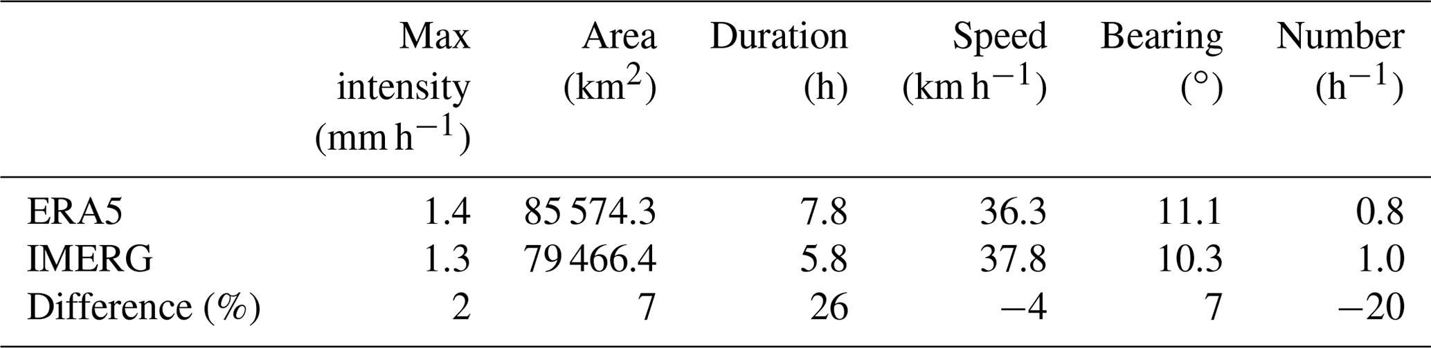
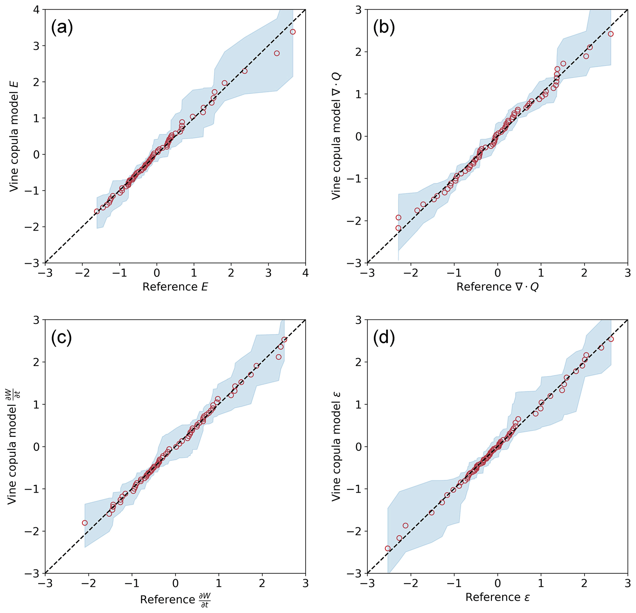
Figure 5 Q–Q plots of standardized atmospheric water balance components between vine copula simulations and reference data from the storm catalog in the Arkansas-Red Basin with a storm area of 25 000 km² and a duration of 2 h. The red circle denotes the mean of simulated values with the reference data at the same percentile. Blue shading denotes the spread of simulations from bootstrapping.

4.2 Goodness-of-fit of the vine copula model

Goodness-of-fit of the vine copula models was assessed by comparing model simulations with reference data from the annual maximum storm catalogs. Quantile–quantile (Q–Q) plots were used to compare water balance components from reference data against simulated values at the same quantile. The simulations here were generated from 100 bootstrap realizations with a sample size of 70. By examining the Q–Q plots of all the 144 cases, we found that the points of reference values and mean simulations fall approximately on the diagonal line, indicating satisfying model fitting (see Fig. 5 for one example). The good fitting is also supported by Pearson's correlation coefficients between sorted reference data and mean simulations. The mean correlation coefficient is 0.995 for E, 0.992 for ∇⋅Q, 0.997 for $\frac{\partial W}{\partial t}$, and 0.993 for ε, with standard deviations of 0.005, 0.005, 0.002, and 0.007, respectively.

We compared copula-simulated precipitation annual maxima against the reference ERA5 precipitation annual maxima from each storm catalog. The ARI of the reference and simulated precipitation was estimated using the Cunnane plotting position. An example of one storm catalog can be seen in Fig. 6; a GEV distribution fitted to the ERA5 precipitation annual maxima using L moments is also shown. Both the univariate GEV and vine copula models can describe the distribution of reference precipitation, with copula estimates slightly exceeding those of the GEV – and cleaving more closely to the reference – for recurrence intervals above 10 years. By examining all 144 storm catalogs, we found that both vine and GEV models agree well with the empirical distributions of the reference data. Good agreement between the model and reference data is also supported by small RRMSEs with a mean of 3 % and a standard deviation of 1 %, indicating that the vine model can depict the dependence structures between atmospheric water balance components to generate realistic precipitation ARIs.

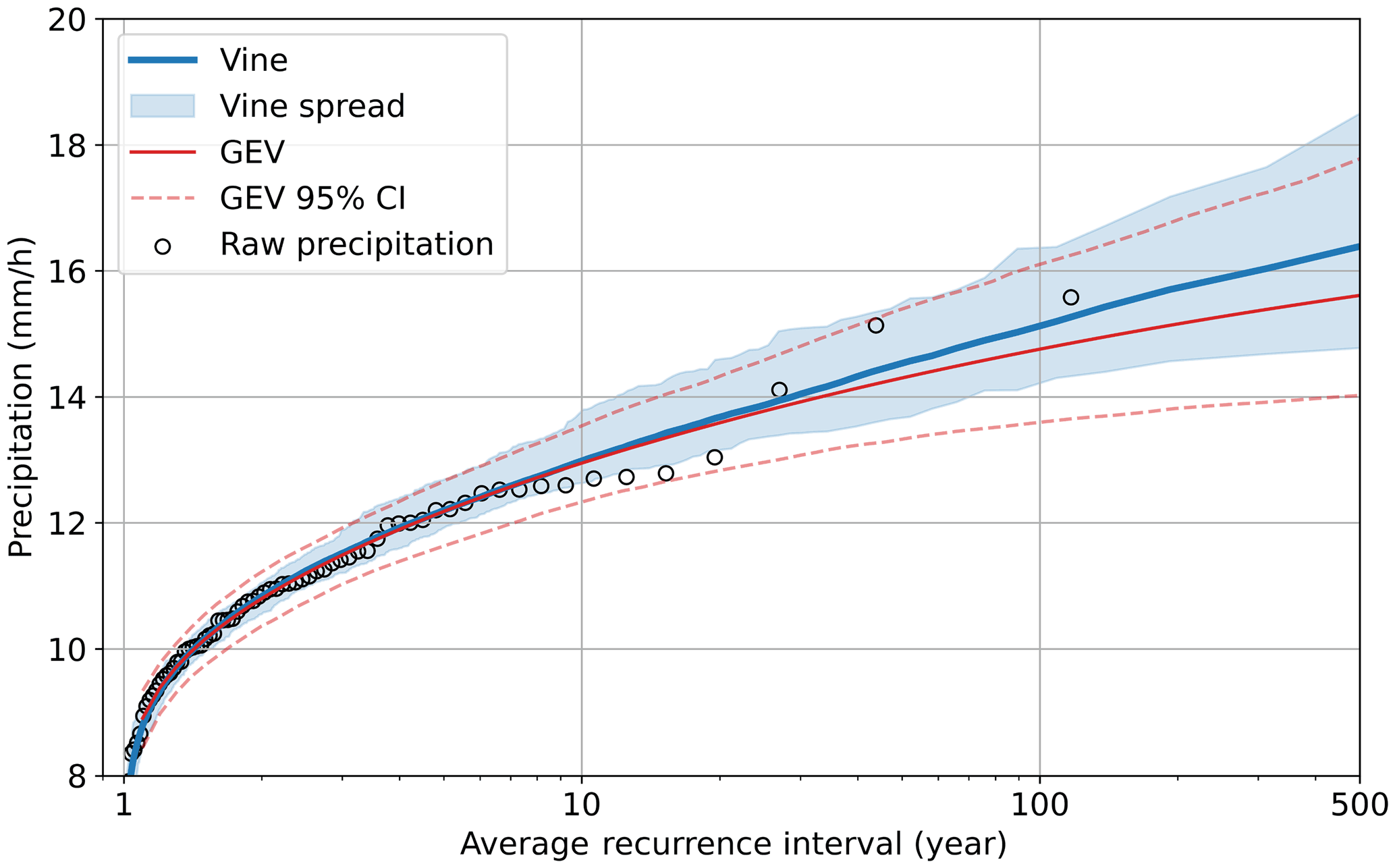
Figure 6 Comparison of estimated return levels of precipitation between vine copula and GEV models in the Arkansas-Red Basin with a storm area of 25 000 km² and duration of 2 h.

4.3 Recurrence interval estimates of the vine copula model

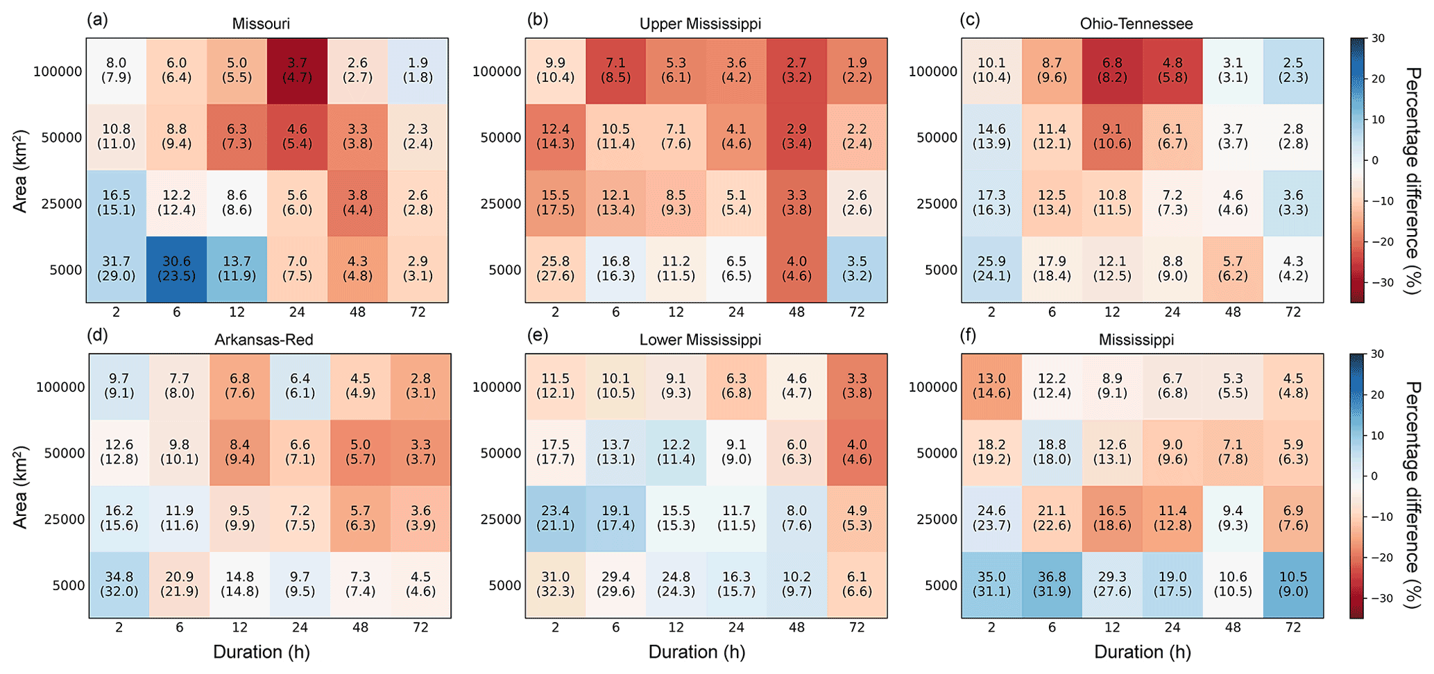
100-year precipitation rate return levels from the vine copula and univariate GEV models were calculated for all 144 storm catalogs (Fig. 7; results of 10-year and 500-year return levels are also shown in Figs. A1 and A2 in Appendix A, respectively). As expected, the precipitation rate decreases with increasing storm area and duration. The storm catalog for the entire Mississippi Basin yields the overall highest precipitation estimates, varying from 3.8 to 31.0 mm h⁻¹, depending on the storm area and duration; this is to be expected since the storm catalog consists of the most extreme storms from all individual subbasins. The Lower Mississippi Basin is the wettest subbasin, with precipitation ranging from 2.9 to 28.8 mm h⁻¹. Estimates generally decrease for subbasins farther away from the Gulf of Mexico's moisture supply. The 100-year precipitation rate from the vine models agrees well with that from the GEV, with the percentage difference on average less than 4 %. Generally, the vine model estimates are higher than GEV for 100-year storms with durations  ≤ 12 h or area ≤ 25 000 km². The difference between the two models grows as ARI increases (see Figs. A1 and A2).

Figure 7 Estimated 100-year precipitation rate (mm h⁻¹) by vine copula and univariate GEV models. GEV estimates are shown in parentheses. The background color denotes the percentage difference between vine copula and GEV estimates.

100-year DAD relationships based on vine copula estimates for the Upper Mississippi Basin are shown in Fig. 8a. At the 5000 km² scale, the precipitation depth increases by 105 % (21 %) from 2 to 6 h (48 to 72 h). When the area grows from 5000 to 100 000 km², the difference between 72 and 2 h depths reduces from 165 to 107 mm. For a fixed duration, the depth decreases quickly between 5000 and 25 000 km² and then slowly until reaching 100 000 km². For 72 h storms, the depth decreases by 41 % (210 to 124 mm) from 5000 to 100 000 km², while for 2 h storms, the decrease is 61 % (45 to 18 mm).

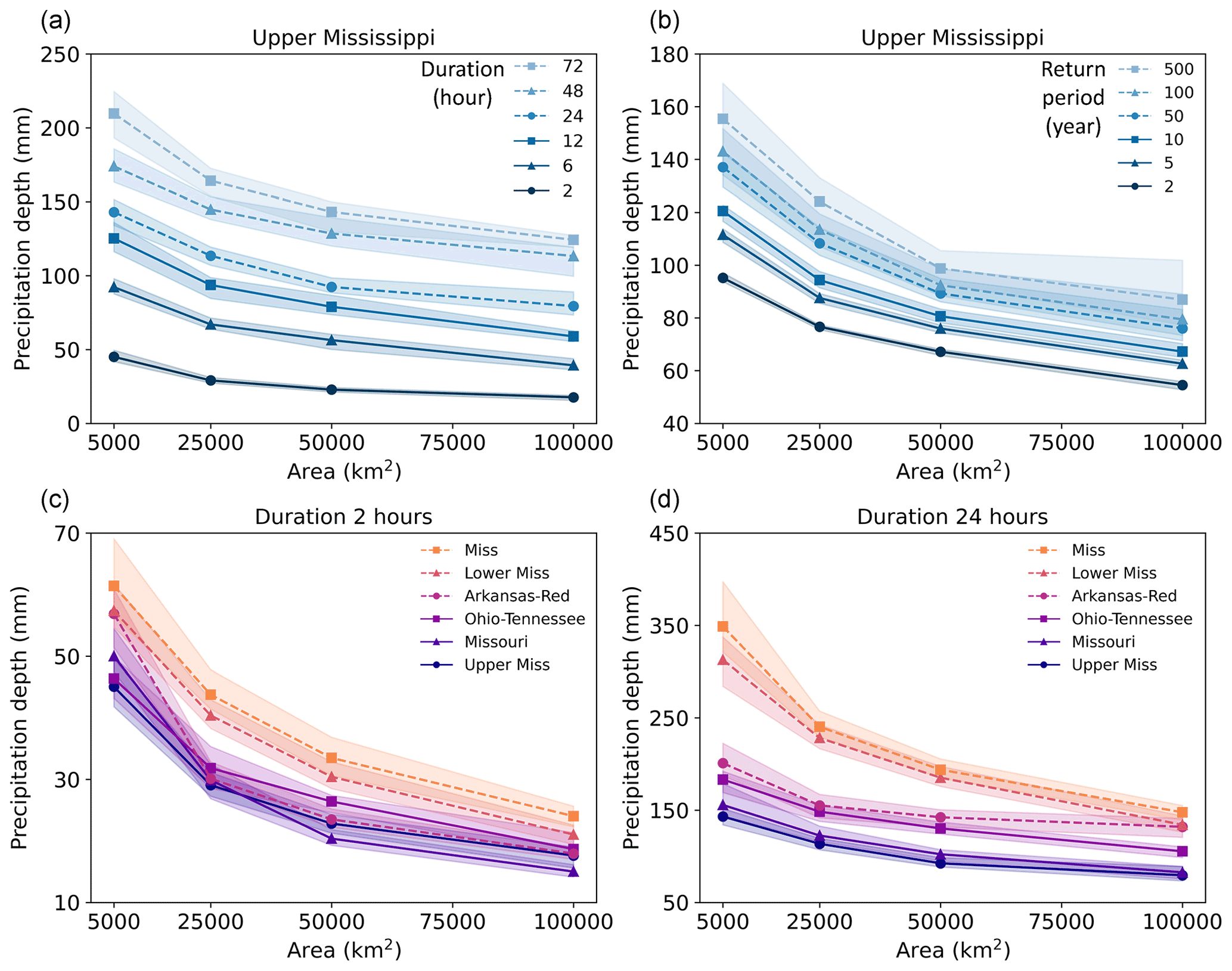
Figure 8 Estimated DAD curves. (a) Upper Mississippi basin with 100-year ARI and different durations. (b) Upper Mississippi basin with the duration of 24 h and different ARIs. (c) Comparison between subbasins with 2 h duration and 100-year ARI. (d) Comparison between subbasins with 24 h duration and 100-year ARI. Markers denote the mean precipitation depth with the specific area. Shading denotes the spread of model estimates.

Our approach can characterize the areal distributions of storm precipitation at different frequency levels. Figure 8b shows depth–area relationships for 24 h storms with ARIs ranging from 2 to 500 years in the Upper Mississippi Basin. The precipitation estimates are the highest at 5000 km², ranging from 95 mm (2-year ARI) to 155 mm (500-year ARI). Such a difference between 2-year and 500-year depths decreases as the area increases. The reduction in precipitation depth with increasing area (i.e., the slope of line segments connecting different areas) is relatively consistent across all ARIs. This suggests that area–depth relationships tend to be independent of storm recurrence intervals. Similarly to other types of statistical models of extremes, the uncertainties increase with ARI (also shown in Fig. 6).

We also compared DAD relationships across subbasins. Figure 8c and d shows the precipitation estimates for 2 and 24 h storms with 100-year ARI in the six basins. Many of these largest storms are from the Lower Mississippi Basin. At the 2 h duration, the overall Mississippi Basin has depth estimates between 24 mm (100 000 km²) and 61 mm (5000 km²), followed by the Lower Mississippi Basin ranging from 21 to 57 mm. The depth in the Arkansas-Red Basin is 57 mm at 5000 km², dropping to 30 mm at 25 000 km² and 18 mm at 100 000 km². The remaining three subbasins have similar results of 15–19 mm at 100 000 km² and 45–50 mm at 5000 km².

Subbasin differences between the DAD curves are more substantial at the 24 h duration (Fig. 8d). Akin to the 2 h duration, Mississippi and Lower Mississippi Basins have similar curves and higher precipitation than the other subbasins. The 24 h duration curves for the Arkansas-Red and Ohio-Tennessee Basins are similar, while Missouri and Upper Mississippi Basins are quite close. Overall, the differences in DAD relationships indicate strong spatial heterogeneity of extreme storms inside the Mississippi Basin, presumably stemming from distance to significant moisture sources.

4.4 Atmospheric water balance in extreme storms

4.4.1 Magnitude of water balance components

This section provides a deeper examination of ERA5 water balance components used in the vine copula model. ∇⋅Q represents the water vapor supply from nearby regions. Recall that a negative value – which is the case in all catalogs – indicates that water vapor is moving into the storm (i.e., convergence). The divergence term has the highest magnitude, indicating its central role in extreme precipitation (Fig. 9a). The mean (standard deviation) of divergence decreases from −9.1 to −3.5 mm h⁻¹ (6.7 to 1.9 mm h⁻¹) with increasing area and decreases from −12 to −2 mm h⁻¹ (5.5 to 0.6 mm h⁻¹) with increasing duration, reflecting the reality that very high rates of water vapor inflow cannot be sustained over large areas or long periods.

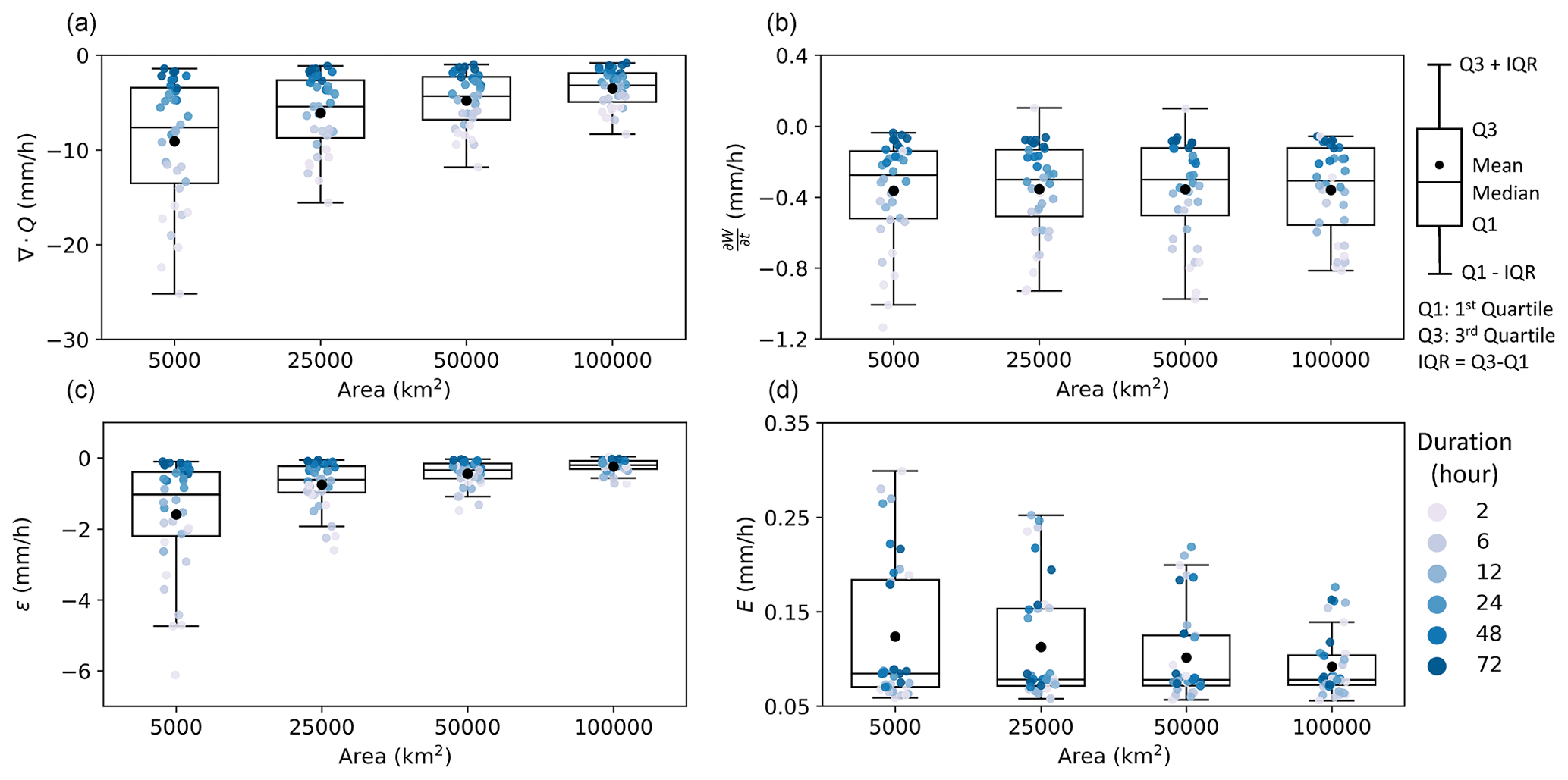
Figure 9 Boxplots of the average water balance components. Points show the average of the water balance components from each storm catalog, with colors denoting storm durations.

The sum of $\frac{\partial W}{\partial t}$ and ε constitute an average of 17 % of precipitation, with some cases reaching as high as 35 %; $\frac{\partial W}{\partial t}$ is negative in most cases (Fig. 9b), indicating that water vapor is “lost” to precipitation. The term does not vary with storm area, remaining around 0.3 mm h⁻¹. However, the mean (standard deviation) of $\frac{\partial W}{\partial t}$ does decrease with duration, from −0.6 (0.4) mm h⁻¹ at 2 h to −0.08 (0.02) mm h⁻¹ at 72 h. For longer durations, the mean approaches zero, which is consistent with the expectation of the long-term atmospheric water balance (Gutenstein et al., 2021).

As mentioned in Sect. 3.3, the residual ε is introduced to compensate for the imperfect closure of atmospheric water balance in ERA5. Most residual terms are negative, indicating that the sum of E, ∇⋅Q, and $\frac{\partial W}{\partial t}$ tends to be higher than ERA5 precipitation. The residual constitutes 10 % of the precipitation on average. As shown in Fig. 9c, ε is the highest at 5000 km², with a mean (standard deviation) of −1.6 (1.6) mm h⁻¹. The mean (standard deviation) decreases to −0.2 (0.2) mm h⁻¹ at 100 000 km². The residual also decreases with increasing duration. For 2 h storms, the mean (standard deviation) is −1.6 (1.6) mm h⁻¹, while for 72 h storms, the mean (standard deviation) is −0.12 (0.09) mm h⁻¹.

Contrary to long-term water balances (Berrisford et al., 2011; Gutenstein et al., 2021), the evapotranspiration term for extreme storms is small at around 3 % of precipitation (Fig. 9d). The mean of the evapotranspiration rate decreases from 0.12 to 0.09 mm h⁻¹ with increasing area, and the standard deviation decreases from 0.08 to 0.03 mm h⁻¹ (though the median is relatively constant with area). There is no clear relationship between E and storm duration.

4.4.2 Dependency structure of moisture balance components

Kendall's τ nonparametric rank correlation coefficients (Abdi, 2007) were computed between all water balance components for each of the 144 storm catalogs. The means and standard deviations of these correlations are shown in Table 4. The strongest correlation of −0.64 is found between divergence and precipitation. The divergence term also shows a relatively strong correlation of 0.42 with the residual term. Evapotranspiration is unrelated to the other components, with mean correlations less than 0.1. The correlations between the time derivative term and the residual (precipitation) are also very weak, with average coefficients of 0.07 (−0.05), respectively. We repeated this correlation analysis based on vine copula model simulations, finding very similar results to Table 4 (results not shown).

Table 4 The mean and standard deviation (in parenthesis) of Kendall's τ correlation coefficients between water balance components. For each of the 144 storm catalogs, Kendall's τ correlation coefficient was computed between two components; the means and standard deviations shown here were obtained from Kendall's τ from all the storm catalogs.

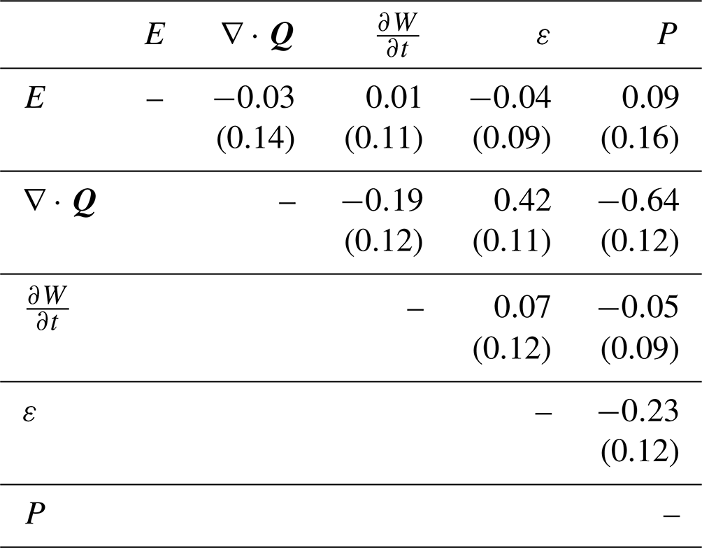
Figure 10 The absolute values of correlation coefficient τ between water vapor components according to (a) area and (b) duration. Points are the absolute values of τ based on each of the annual maximum storm catalogs. Diamonds show the mean of all the computed τ; error bars show the 95 % confidence interval of the mean.

We further examined how correlations between water vapor components depend on storm area and duration (Fig. 10). The average correlation coefficient between the divergence and time derivative term increases with storm area (Fig. 10a), while exhibiting a more complex pattern for duration – increasing from 0.21 at 2 h to 0.24 at 24 h and then decreasing to 0.15 at 72 h (Fig. 10b). For the divergence and the residual terms, the mean correlation drops from 0.5 to 0.34 with increasing area and from 0.46 to 0.35 with increasing duration. The average correlation between the divergence and precipitation terms decreases from 0.69 to 0.58 with increasing area while rising from 0.49 at 2 h duration to 0.75 at 72 h duration. The average correlation between the time derivative and residual terms shows a modest reduction from 0.13 to 0.08 with increasing area, and a larger drop, from 0.29 to 0.17, with increasing duration. The average correlation between residual and precipitation terms drops from 0.29 to 0.17 with increasing area, while it increases from 0.18 at 2 h to 0.27 at 24 h and drops to 0.23 at 72 h duration. In short, there are complex relationships among water balance components that depend on storm spatiotemporal scale and cannot be ignored in any attempt at modeling their joint roles in extreme precipitation.

The correlation analyses shown in Table 4 and Fig. 10 are imperfect representations of the dependency structure between water balance components, since correlation coefficients distill bivariate distributions into a single number. The vine copula, on the other hand, can capture such structures. More detailed relationships can be seen by plotting the simulation results from the vine copula model. Figure 11 shows an example – the 25 000 km², 2 h storm catalog for the Arkansas-Red Basin. The lower portion of the plot shows the conditional distribution of one water balance component for a fixed value of a second component, with the red line showing the median and the shaded contours denoting deciles. Nonlinear relationships can be seen in ε vs. ∇⋅Q, ε vs. $\frac{\partial W}{\partial t}$, and ε vs. P. Note that the correlation coefficients for $\frac{\partial W}{\partial t}$ vs. ε and $\frac{\partial W}{\partial t}$ vs. P are 0.30 and −0.23, respectively, which is much higher than the averages of 0.07 and −0.05 from Table 3. This highlights that considerable variability exists in the dependency relationships across the many storm catalogs, linked to storm region, area, and duration.

Figure 11 Bivariate dependency structure of simulated atmospheric water balance components from the 25 000 km², 2 h duration storm catalog for the Arkansas-Red Basin. Histograms along the diagonal show the marginal distributions of the individual components. Panels below and left of the diagonal show variation in copula simulations of one water balance component conditioned on another component, with the red line denoting conditional median and blue shading denoting deciles. Panels above and to the right of the diagonal shows Kendall's τ correlation coefficients between components.

The histograms along the diagonal show the marginal distributions of each water balance component used in the vine copula model; the divergence term's histogram is smooth due to the use of a GEV marginal distribution, while the other three components used empirical CDFs. We used empirical CDFs for the remaining variables to reduce additional parameters and errors introduced by fitting parametric distributions; this is common practice in vine copula modeling. However, empirical CDFs can constrain the simulated variables to their maximum in the original sample data, leading to unrealistic upper-bounded tail behavior. Therefore, we used GEV distribution to fit the dominant component (i.e., the convergence term) to allow the model to generate extreme precipitation that exceeds the original maximum. Note that it is feasible to fit parametric distributions to all atmospheric water balance components. The influence on the results is rather minor as long as the parametric distribution fits to each component are good. For example, the distribution of the residual term can be fitted by a t-distribution, while the time derivative and evapotranspiration terms can be fitted with beta distributions. Another advantage of using parametric distribution is that nonstationarities (e.g., changing location and scale) in each atmospheric water balance component can be modeled with distribution parameters that vary with time or other climate indices (see Sect. 5.5).

5 Discussion

5.1 Residual in the atmospheric water balance

The residual term ε is introduced in our study to close the atmospheric water balance of reanalysis data, which can affect precipitation estimates. Mass balance errors could come from the data assimilation (DA) scheme and the change of observation systems within ERA5 Reanalysis (Mayer et al., 2021; Lewis et al., 2019). Studies have also shown that the differencing method to compute the water vapor flux divergence is another major source of error (Mayer et al., 2021; Gutenstein et al., 2021; Seager and Henderson, 2013). Nonetheless, the average residual is about 10 % of the precipitation for all cases, indicating that the ERA5 shows relatively good water balance closure for extreme events in the Mississippi Basin. The residual term is the greatest for 5000 km² and 2 h storms and approaches zero as duration and area increase. Compared with the univariate model fitted solely on precipitation, the multivariate vine copula model allows us to explicitly include the residual term and model its dependence structures with other components. In future work, comparisons could be made between vine copulas fitted based on reanalysis and climate models. The latter class of simulations is not subject to DA-related mass balance violations and, thus, could help to identify the dominant sources of water balance closure error (i.e., DA or differencing).

5.2 Uncertainty and bias in ERA5 reanalysis

ERA5 Reanalysis is based on numerical weather forecasts combined with multiple observations and is subject to multiple error sources, including numerical model errors, observation errors, DA errors, and spatiotemporal heterogeneity of data sources (Bosilovich et al., 2008; Nogueira, 2020). As a result, precipitation bias exists in ERA5 over the study region, which can influence our model estimates. Previous studies have shown discrepancies in precipitation climatology between ERA5 and observations over the CONUS. We performed an additional comparison with interpolated gauge-based precipitation fields, supporting that ERA5 underestimates extreme precipitation in the Mississippi Basin (see Appendix B). The underestimation may be related to insufficiently strong water vapor flux divergence, given its primary role in extreme storms and high correlation with precipitation as described in Sect. 4.4. Also, the coarse spatial and temporal resolution of ERA5 may limit its ability to represent small-scale, short-lived convective storms that generate extreme precipitation (Beck et al., 2019; Ebert et al., 2007). Studies have also mentioned precipitation bias coming from orography smoothing and inadequate observations over mountainous areas (Essou et al., 2017; Jiao et al., 2021). Overall, one must be careful when analyzing extreme storms based on reanalysis, since the accuracy can vary greatly in space and time depending on topography, climate region, and the quantity and quality of assimilated observations (Ebert et al., 2007; Essou et al., 2017; Zhang et al., 2018).

Uncertainties also exist in atmospheric water balance components in ERA5 Reanalysis and can influence the precipitation estimates from the vine copula model. Uniquely among reanalyses (to the best of our knowledge), ERA5 includes coarser-resolution (3 h, 0.5^∘ grid scales) ensembles that can be used to examine some forms of uncertainty. To assess these uncertainties, we computed the water balance components in the annual maximum storm catalogs based on 10 ERA5 ensemble members (results not shown). These ensembles estimate the uncertainties of observations in DA and model parameterizations (Hersbach et al., 2020). All the atmospheric water balance components showed certain variations, especially for precipitation and water vapor flux convergence. Nevertheless, the coarser resolution of the ensemble members smooths out high precipitation regions and periods and result in different storm tracking and search results, making it difficult to use these to quantify the uncertainty in our precipitation estimates. However, the variability in ERA5 ensemble members can still qualitatively reflect the uncertainty in atmospheric variables across different subbasins and different storm spatiotemporal scales. Other reanalysis or numerical models, such as MERRA-2 (Gelaro et al., 2017; Moalafhi et al., 2017), can also be alternative sources to evaluate the uncertainty in ERA5 reanalysis. For a valid comparison, a common period of these datasets (e.g., 1980–2020) and transformation to the same spatial-temporal resolution are needed to perform storm tracking and vine copula fitting. An ensemble distribution can be generated from extreme precipitation estimates based on each dataset. It is expected that the variability of the precipitation estimates would increase by incorporating multiple reanalysis/numerical models.

5.3 Connection to DAD and area reduction factors

Our “storm-centered” approach allows the estimation of precipitation frequency for a specific area and duration within a region (as shown in Sect. 4.3). This constitutes an alternative way to approach the long-standing task of deriving DAD relationships, i.e., describing how extreme precipitation depth varies with averaging area and duration, usually for the purpose of flood analysis (Alexander, 1963; USACE, 1945; Weather Bureau, 1946). It should be noted, however, that the derivation of DAD from individual storms has generally not been extended to recurrence intervals as is done here (e.g., in Fig. 8). The one notable exception that we are aware of is stochastic storm transposition (Alexander, 1963; Foufoula-Georgiou, 1989; Wright et al., 2020). Our method – which can produce ARI estimates associated with DAD relationships – shares SST's focus on storm catalogs (Wright et al., 2013; Zhou et al., 2019). While it is not the primary focus of this study, we show the potential of the “storm-centered” idea to address the old question of DAD relationships, with the help of advancements in precipitation products and storm tracking methods.

Both DAD and our approach also share a connection to area reduction factors (ARFs), which are fractions between zero and 1 that depict the ratio of the average precipitation depth over an area to a point-scale precipitation depth, given a fixed duration. DAD and ARF are highly related concepts, despite serving somewhat different purposes. ARFs are used to convert gauge-based (i.e., point-scale) precipitation frequency estimates to areal estimates of the same ARI and duration (e.g., Kao and Deneale, 2021; Miller, 1964; Olivera et al., 2008). Most ARF studies have tried to obtain such ratios using a “fixed-area” approach, i.e., to relate precipitation depth from point to area at a fixed location (e.g., Asquith and Famiglietti, 2000; Breinl et al., 2020; Durrans et al., 2002), though others have argued that storm-centered ARF approaches are more conceptually valid (Kim and Kang, 2017; Thorndahl et al., 2019; Wright et al., 2014). The ability to derive storm-centered DAD relationships using our method can, in principle, obviate the need for ARFs entirely, something that has been advocated previously (Wright et al., 2014). To support this point, we compared vine copula DAD curves with those estimated by the ARFs from Kao et al. (2020) in the Ohio River Basin at 10-year ARI (see Appendix C and Fig. C1). The vine copula DAD estimates agree well with those ARF estimates for storm duration between 6 and 72 h, while for 2 h storms, the vine copula estimates are more conservative, i.e., the precipitation depth reduces much more slowly with increasing area. Such discrepancies may be attributable to the ARF estimation of Kao et al. (2020) being a “fixed-area” approach, i.e., the precipitation depth is compared to areal depth in a watershed. Nevertheless, the number of large watersheds in the Mississippi Basin (e.g., watersheds greater than 50 000 km²) is limited, which may limit the approach's ability to identify truly areal maxima, especially for short-duration large-area storms. This suggests that our “storm-centered” approach may provide more conservative DAD relationships for storms with short durations. An alternative explanation, however, could be that these differences highlight the limits of ERA5 in depicting extreme convective rainfall at small space-time scales. Another contention within the ARF literature is whether or not such ratios are independent of recurrence intervals (e.g., Greener and Roesch, 1997; Osborn et al., 1980; Pavlovic et al., 2016). Relevant to this debate, we found that DAD appears to be independent of recurrence intervals for 5000–100 000 km² scales in the Mississippi Basin.

5.4 Interpretation of average recurrence intervals

The ARI is conventionally interpreted as the expected time interval (in years) between events exceeding a certain magnitude at one specific location (Coles, 2001; Serinaldi, 2015). On the contrary, our “storm-centered” approach identified all the storms at different locations within the basin to create annual maximum storm catalogs. As a result, the ARI estimates in our study describe the probability that an extreme storm will happen somewhere within a region (e.g., the Mississippi basin or subbasin), while the storm location is not specified. Examples of equivalent formulations of ARI can be found in Bosma et al. (2020) and Zhu et al. (2013). Moving from this formulation to the computation of ARIs at one specific site (e.g., a watershed) requires one to model the storm spatial arrival process, which describes the probability that the extreme storm “hits” the chosen site (e.g., Nathan et al., 2016; Wilson and Foufoula-Georgiou, 1990; Wright et al., 2020). The arrival process is challenging because the storm occurrence rate can vary greatly across a region due to inhomogeneous precipitation properties (e.g., Wilson and Foufoula-Georgiou, 1990; Wright et al., 2020; Yu et al., 2021). One simplification is to assume that storm position is independent of storm characteristics, and the storm center is equally likely to occur within the basin (Alexander, 1969; Foufoula-Georgiou, 1989). Then, the exceedance probability at a specific watershed within the basin can be written as

$$\begin{array}{}\text{(14)}& P_{\mathrm{c}}(X>x)={\displaystyle \frac{A_{\mathrm{c}}}{A_{\mathrm{s}}}}\cdot P_{\mathrm{s}}(X>x),\end{array}$$

where P_c(X>x) is the exceedance probability of precipitation X at the specific watershed, A_c is the watershed area, A_s is the basin area where the annual maxima storm catalog is built, and P_s(X>x) is the exceedance probability obtained based on the vine copulas model in this study. More complex arrival formulations could consider watershed shape and orientation (Wright et al., 2013). Such arrival processes could be realized using stochastic models (Foufoula-Georgiou, 1989; Wilson and Foufoula-Georgiou, 1990; England et al., 2014) or Monte Carlo simulations (Wright et al., 2013; Zhou et al., 2019; Yu et al., 2021) but are beyond the scope of this study.

5.5 Nonstationarity in multivariate models

Changes in annual and extreme precipitation due to anthropogenic climate change in the Mississippi Basin have been observed and investigated in many studies (e.g., Karl and Knight, 1998; Groisman et al., 2004; Pan et al., 2016; Gori et al., 2022), with important implications for precipitation frequency estimates (e.g., Milly et al., 2008; Bender et al., 2014; Zscheischler et al., 2018). For multivariate distribution models (e.g., copulas), nonstationarities may exist in the marginal distributions of random variables or their relationships, i.e., dependency structures (Xu et al., 2020). Our approach can consider nonstationarities by using marginal distributions and dependence structures with parameters that vary as a function of, e.g., time, temperature, or climate indices in vine copulas (for examples, see Bender et al., 2014; Jiang et al., 2015; Sarhadi et al., 2018; Xu et al., 2020). This attribute gives our method more flexibility to analyze extreme storm frequency in a changing climate, especially to reveal nonstationary relationships between moisture components. Nevertheless, we expect high uncertainties when using nonstationary models due to statistical issues (Serinaldi and Kilsby, 2015) and a lack of clarity around precipitation change across gridded precipitation datasets (Mallakpour et al., 2022). Therefore, multi-model trend comparison and careful interpretation are necessary components for nonstationary modeling (Mallakpour et al., 2022), especially when using reanalysis that exhibits substantial inter-model variability (Alexander et al., 2020). As mentioned above, such modeling is potentially within reach of our framework but is beyond the scope of this study.

6 Summary and conclusions

In the study, we present a storm-centered multivariate copula model based on the atmospheric water balance equation to estimate the frequency of extreme spatiotemporal precipitation. The model was applied to extreme precipitation within the Mississippi Basin. Two-dimensional storm objects were identified using the storm tracking and regional characterization (STARCH) method applied to ERA5 precipitation fields over the contiguous United States from 1951 to 2020. STARCH identified storm objects at each time step, then merged them across time to track storms. Afterward, an area–duration selection algorithm was used to extract the largest storms from each year with specific areas and durations in order to create “storm catalogs”, each of 70 annual maxima. Selected areas were 5000, 25 000, 50 000, and 100 000 km², and durations were 2, 6, 12, 24, 48, and 72 h. This selection process was applied to the whole Mississippi Basin and its five major subbasins, resulting in 144 storm catalogs. Using the STARCH method, the spatiotemporal properties of ERA5 storms were validated against the observation-based IMERG precipitation dataset, showing good consistency.

The annual maximum precipitation distribution was represented using a joint distribution of atmospheric water balance components: land surface evapotranspiration, water vapor flux divergence, the time derivative of water vapor storage, and a residual error term. The latter was included to account for imperfect water balance closure in ERA5. Within each storm catalog, water balance components from ERA5 were computed for each annual maximum storm object and fitted to a multivariate vine copula model. This model used a GEV marginal distribution for the divergence term and empirical distributions for the other components. The fitted model was then used to simulate samples of water balance components to calculate the associated precipitation via the water balance equation. The frequency of annual precipitation maxima was then estimated nonparametrically based on these simulations. The following conclusions can be drawn:

It is feasible to generate plausible extreme precipitation estimates from a vine copula model that incorporates additional physical information from the atmospheric water balance. Good fits were found based on Q–Q plots and comparisons of estimated ARI against those from more conventional univariate GEV distributions fitted to ERA5 precipitation. This indicates that the copula approach can represent the complex dependence structures between water balance components. Percentage differences between the vine copula and univariate GEV models were on average less than 4 % for the 100-year ARI but increased for rarer quantiles.

Among water balance components, water vapor flux divergence is the dominant term in extreme precipitation. Land surface evapotranspiration plays the smallest role, constituting about 3 % of precipitation. The sum of the time derivative of precipitable water and residual terms constitute an average of 17 % of precipitation. Nonlinear dependencies among water balance components vary with storm region, area, and duration; these cannot be neglected when modeling their joint roles in extreme precipitation.

Prior studies have shown that, due to data assimilation and numerical methods, the atmospheric water vapor mass in ERA5 is not perfectly conserved. Despite this, we found relatively good atmospheric water balance closure for extreme events in the Mississippi Basin, with the residual on average constituting about 10 % of precipitation. To our knowledge, this is the first study that examines atmospheric water balance closure for precipitation extremes in reanalysis data. The residual term is the greatest in the 5000 km² and 2 h storm catalogs and approaches zero as duration and area increase. Users need to treat the residual carefully when examining extreme precipitation from reanalysis (and possibly other atmospheric simulations such as climate models), especially for short durations and small spatial scales.

Despite the advancement in numerical and data assimilation schemes, ERA5 is still subject to model bias; it tends to underestimate extreme precipitation over the Mississippi Basin. This bias may be attributable to the inadequate simulation of water vapor flux divergence due to its dominant role in precipitation extremes. Also, coarse spatiotemporal resolution and limited observations for assimilation over mountainous areas can contribute further to precipitation biases.

Overall, rainfall frequency analysis can benefit from utilizing additional information from atmospheric/land surface processes. Compared with the conventional approach, the vine copula model allows an explicit representation of the dependence structures between atmospheric water balance components and enables us to investigate the main driver of extreme precipitation. The model does not need an explicit parametric form for the tail of the precipitation distribution, as it is determined by the tail of the moisture components and their dependence structures. This dependence structure can also serve as a constraint that prevents unrealistic large estimates (Bevacqua et al., 2017). Though not explored here due to the complications in interpreting the results (e.g., nonstationary ARIs), the approach is also able to accommodate nonstationary conditions by incorporating marginal distributions and dependence structures that vary with time or according to other climate predictions (e.g., temperature or climate indices, see Bender et al., 2014; Sarhadi et al., 2018; Xu et al., 2020).

Our “storm-centered” approach enables us to focus on the major extreme storms over a region, notwithstanding ERA5's tendency to underestimate those extremes. This feature contrasts with more typical gauge-based analyses that may restrict the number of extreme events due to a limited sampling area. By preserving the spatiotemporal structure of the storms, we can investigate extreme precipitation frequency in user-defined areas. Such areal precipitation estimates demonstrate the potential of using the “storm-centered” idea to derive DAD relationships for storms with different ARIs, with the help of long-term reanalysis products and storm tracking techniques.

The ARIs estimated by our approach represent the frequencies of extreme storms that happen over the entire region. To obtain precipitation ARIs for one specific site within that basin, an additional storm arrival process (i.e., the probability that the storm “hits” the site) is needed to modify the ARI estimates. Such arrival processes can be realized using statistical models or Monte Carlo simulations and will be a direction of future study. Despite evident biases in extreme precipitation, reasonable atmospheric water balance closure can be found in ERA5, lending confidence that it and similar reanalyses can represent reasonable water vapor interactions (Brown and Kummerow, 2014), which can help to understand the mechanisms of extreme events. In the longer run, the performance of this approach can be expected to benefit from further developments in numerical weather simulation and data assimilation.

Appendix A: 10- and 500-year precipitation estimates of the vine copula model

Figure A1 Estimated 10-year precipitation from vine copula and univariate GEV models. GEV estimates are in parentheses.

Figure A2 Estimated 500-year precipitation from vine copula and univariate GEV models. GEV estimates are in parentheses.

Appendix B: Comparison of ERA5 and nClimgrid extreme precipitation

To better assess the bias in ERA5 extreme precipitation, here we provide a comparison between ERA5 Reanalysis and a gauge-based product, the Gridded 5 km GHCN-Daily Temperature and Precipitation Dataset (nClimGrid, Vose et al., 2014), which provides daily precipitation on a 0.05^∘ grid for CONUS by interpolating gauge observations. The nClimGrid data were regridded to 0.25^∘ using the conservative method described in Sect. 2.2 to match ERA5's spatial resolution. To match the temporal resolutions of the two datasets, we shifted the ERA5 time zone from Universal Time Coordinated (UTC) to Central Standard Time (CST) and computed daily precipitation using the daily interval (07:00–06:59) in nClimGrid. ERA5 daily precipitation patterns were generally consistent with those from nClimGrid, suggesting similar storm spatiotemporal properties (results not shown). We computed the difference in the 99th percentile daily precipitation between ERA5 and nClimGrid in the 1951–2020 period, shown in Fig. B1. Basin-average 99th daily precipitation from ERA5 and nClimGrid, and their differences are summarized in Table B1. The ERA5 99th percentile of daily precipitation is on average 8 % lower than that of nClimgrid in the Mississippi Basin, with strong spatial variation across subbasins. Specifically, ERA5 underestimates extreme precipitation in the Lower Mississippi Basin; this underestimation diminishes in areas further inland. On the other hand, ERA5 overestimates precipitation over the mountainous areas in the west Missouri Basin.

Table B1 Comparison of basin-averaged 99th percentile daily precipitation between ERA5 and nClimGrid from 1951 to 2020. The percentage difference is computed by (nClimGrid-ERA5)/nClimGrid × 100.

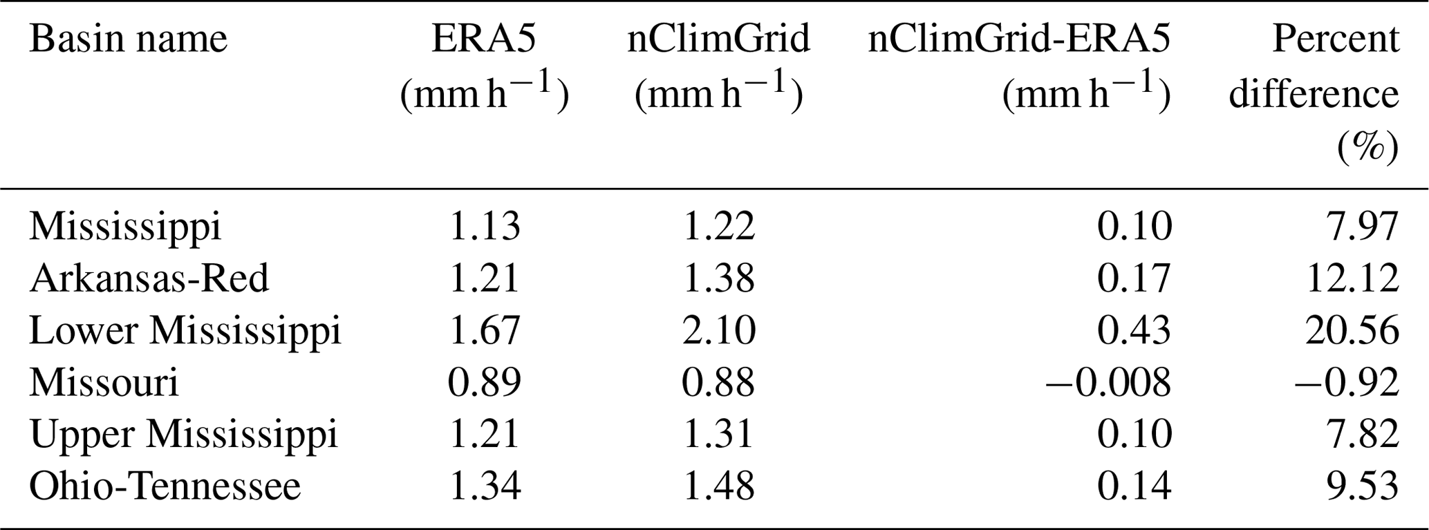
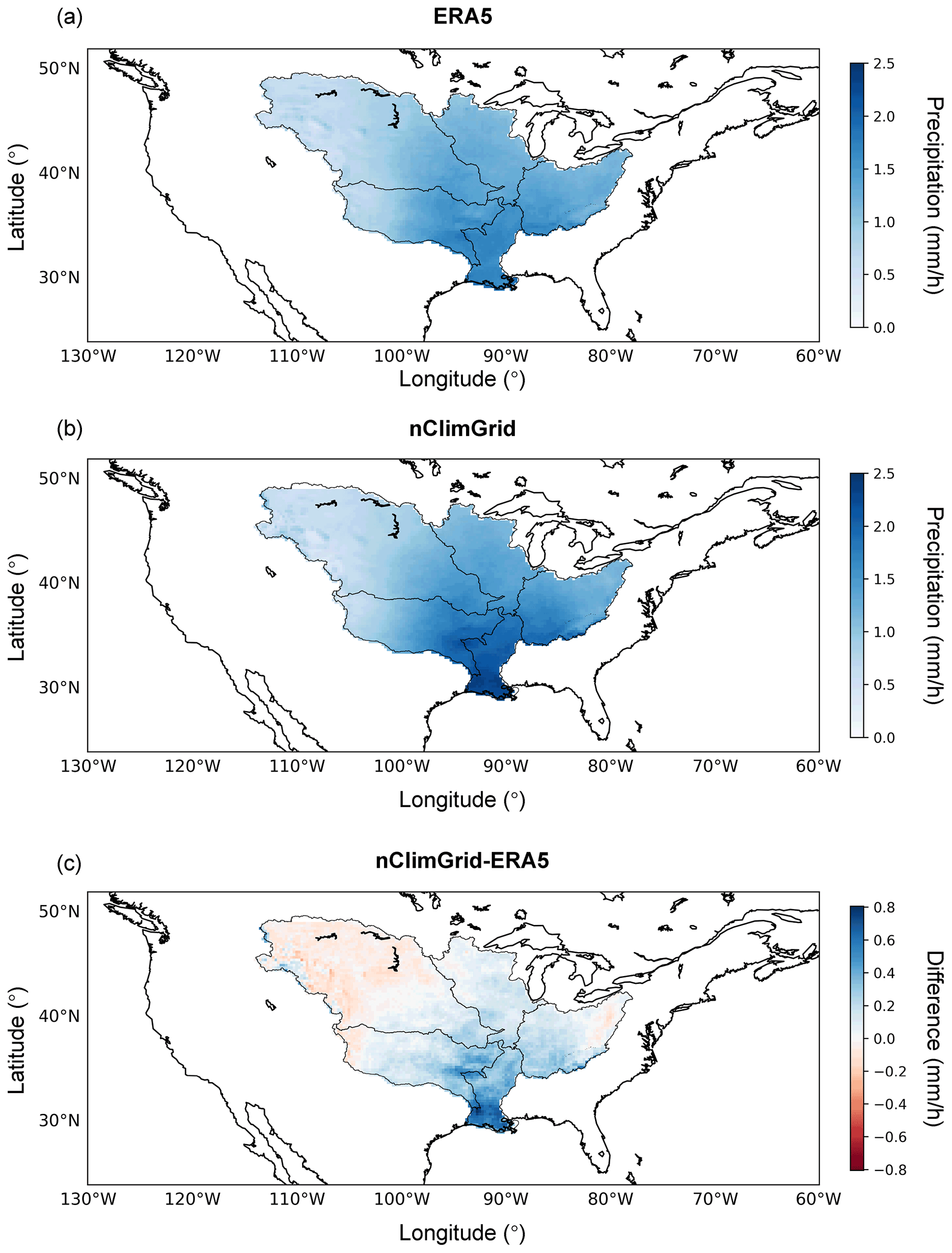
Figure B1 99th percentile daily precipitation during 1951–2020 for (a) ERA5, (b) nClimGrid, and (c) the difference between the two datasets.

Appendix C: Validation of vine copula DAD relationships

The vine copula DAD curve was compared against the ARFs in Kao et al. (2020). The ARFs were estimated for 10-year precipitation with durations of 2–72 h and areas of 10–100 000 km² in the Ohio River Basin, using a watershed-based approach and gauge-based dataset (DSI-3240, National Climatic Data Center, 2003). We calculated new DAD curves by converting the vine copula hourly precipitation depth at 5000 km² to the depths at larger areas based on the ARFs. The new DAD curves were then compared with the original DAD curves estimated from vine copulas, as shown in Fig. C1. More discussion of this figure can be found in Sect. 5.3.

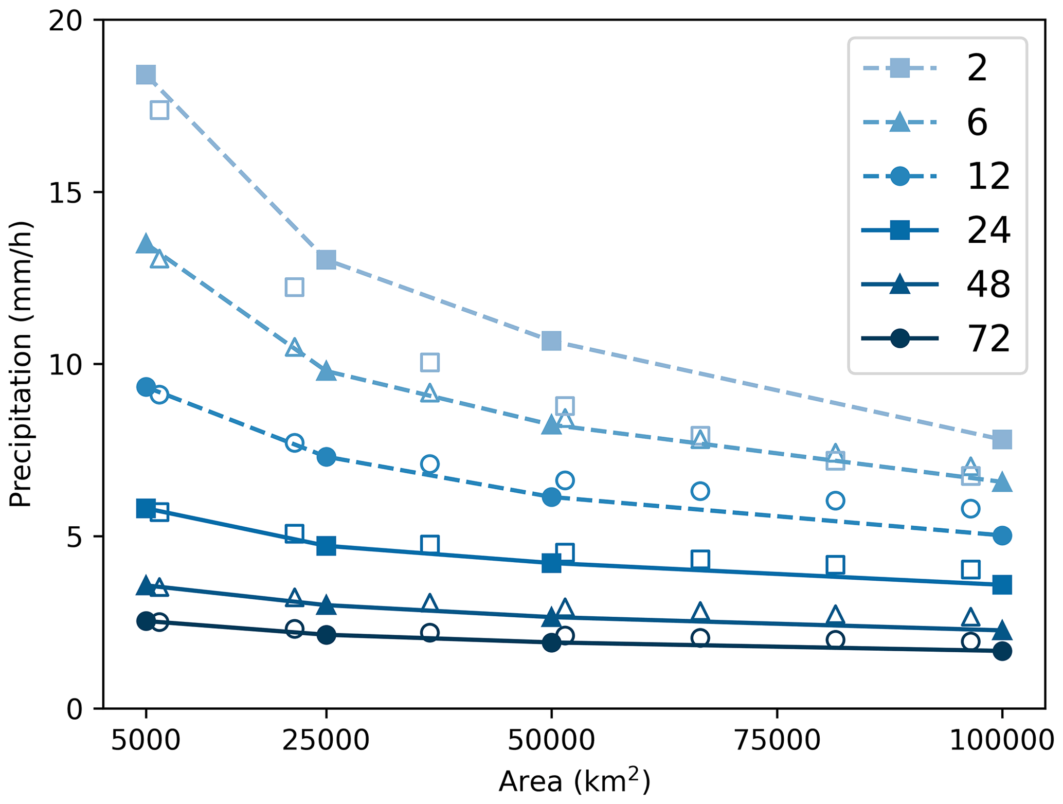
Figure C1 Comparison of DAD curves estimated from vine copulas (solid markers) and ARFs from Kao et al. (2020) (empty makers) for Ohio River Basin with 10-year ARI and 2–72 h durations.