the Creative Commons Attribution 4.0 License.
the Creative Commons Attribution 4.0 License.
 | 11 Oct 2022
Improving hydrologic models for predictions and process understanding using neural ODEs
Andreas Scheidegger
Marco Baity-Jesi
Carlo Albert
Fabrizio Fenicia
Deep learning methods have frequently outperformed conceptual hydrologic models in rainfall-runoff modelling. Attempts of investigating such deep learning models internally are being made, but the traceability of model states and processes and their interrelations to model input and output is not yet fully understood. Direct interpretability of mechanistic processes has always been considered an asset of conceptual models that helps to gain system understanding aside of predictability. We introduce hydrologic neural ordinary differential equation (ODE) models that perform as well as state-of-the-art deep learning methods in stream flow prediction while maintaining the ease of interpretability of conceptual hydrologic models. In neural ODEs, internal processes that are represented in differential equations, are substituted by neural networks. Therefore, neural ODE models enable the fusion of deep learning with mechanistic modelling. We demonstrate the basin-specific predictive performance for 569 catchments of the continental United States. For exemplary basins, we analyse the dynamics of states and processes learned by the model-internal neural networks. Finally, we discuss the potential of neural ODE models in hydrology.
- Article
(3894 KB) - Full-text XML
- BibTeX
- EndNote


1.1 Machine learning in hydrology
Deep learning models, in particular long-short-term memory (LSTM) neural networks, have outperformed traditionally used conceptual models in hydrologic modelling (Kratzert et al., 2018; Feng et al., 2020; Lees et al., 2021). Machine learning methods provide great versatility (Shen, 2018; Shen et al., 2018; Reichstein et al., 2019) and have demonstrated unprecedented accuracy in various modelling tasks like predictions in ungauged basins (PUB; e.g. Kratzert et al., 2019b; Prieto et al., 2019), transfer learning to data-scarce regions (Ma et al., 2021) or flood forecasting (Frame et al., 2022; Nevo et al., 2022). Nonetheless, deep learning remains a field of progress with gaps to fill. Here, we want to focus on three of them that are particularly relevant in hydrology.
First, machine-learning models are still not as easily interpretable as traditionally used physics-based conceptual hydrologic models are (Samek et al., 2019; Reichstein et al., 2019). Although high predictive accuracy is crucial to all modelling tasks, it is often not the only purpose. When dealing with complex systems, as is the case in hydrology, learning about the system and understanding its internal and external interrelations is just as important to many researchers. There have been first attempts in this direction by investigating what happens inside machine-learning models (Kratzert et al., 2019a). Generally, research on explainable artificial intelligence (XAI) or “interpretable machine learning” (e.g. Samek et al., 2019; Montavon et al., 2018; Molnar et al., 2020; Molnar, 2022) has strongly advanced in recent years. Specifically, in hydrologic modelling, ties between internal model states and hydrologic processes are being elicited like the correlation between the dynamics of certain hidden states of LSTM models with measured soil moisture (Lees et al., 2022).
Therefore, it is becoming more and more inaccurate to label machine-learning methods as black box models since techniques exist that shed light on the internal information processing of machine-learning methods (see also Nearing et al., 2021; Lees et al., 2022). Yet, internal investigation of machine-learning models relies on additional methods that come with their own assumptions and caveats, and the current straightforward interpretability of conceptual models serves as a benchmark in the hydrologic community. Much environmental research is dedicated toward extrapolation in space and in time and of boundary conditions, in order to investigate extreme events (Frame et al., 2022), climate change projections (Nearing et al., 2019) and so on. In all these fields, ease of interpretability is desirable.
Second, while the introduction of system memory as a physical principle (like in LSTM models) has turned out to be crucial for hydrograph prediction, other basic physical principles have not necessarily been fulfilled, yet. Currently used machine-learning approaches are limited to fixed time steps, which restricts their usage. For instance, while LSTM approaches have been shown to perform well at the task of discharge prediction on daily resolution in many different cases (e.g. Kratzert et al., 2018, 2019b), high-flow events often occur at a higher temporal resolution. For LSTM models, recent developments show adaptation approaches to finer time intervals, i.e. from daily to hourly (Gauch et al., 2021), or introduce continuous time hidden states within the LSTM framework in order to internally update their step-wise dynamics (Lechner and Hasani, 2020). Yet, thereby, modelling becomes more interlaced, and computational effort increases without increasing system understanding. Despite all the progress in this field, real-world systems with their states and processes are continuous in time, and from a physics perspective, it remains unsatisfactory when models are restricted to certain timescales. Further, attempts to enforce fundamental principles like mass balance were made but showed that this constraint might even worsen predictive power compared to the unconstrained LSTM variants (Hoedt et al., 2021).
Third, there is often prior knowledge that cannot be included in machine-learning models. Data-driven modelling demonstrates impressive abilities in terms of mimicking and/or improving the translation from driving forces variables through the system into its output, like from precipitation to discharge in hydrology. Yet, the question remains as to why such models only have to use data to learn all the internal processes of the system from scratch. Much knowledge about hydrology has been gathered in the past, so why not provide such knowledge, for example, mechanistic structure, reliable causal interrelations and context-specific information (Rackauckas et al., 2020), to the models directly? Of course, the risk impends that certain constitutive relations as they are used in mechanistic processes might be inexact or misleading. Nonetheless, on the one hand we can rely on many basic principles that are generally agreed upon, and on the other hand, including constitutive relations has the potential of providing additional knowledge on hydrological processes aside from data alone.
1.2 Conceptual hydrologic models
For conceptual hydrologic models, these gaps have been mostly closed over the last decades: the development of conceptual bucket-type models (e.g. HBV or GR4J; see Knoben et al., 2020, and references therein) rests on the deductive insight that physical principles do hold in general. Basic building blocks have been elicited, and modular frameworks allow models to be tailored to any task at hand (Fenicia et al., 2011; Clark et al., 2015) while maintaining full interpretability of each element. Knowledge about local conditions is used to improve the models (Gnann et al., 2021), fostering both system understanding and accuracy in predictions (Kirchner, 2006; Fenicia et al., 2014) in typically data-limited modelling tasks (Fenicia et al., 2008; Li et al., 2021).
Yet, there remains a dichotomy between bottom-up and top-down approaches in hydrology (Savenije, 2009; Gharari et al., 2021). In the former, process knowledge that was acquired at smaller scales is generalized to the catchment scale, while in the latter, prediction and interpretation of the hydrologic system are based on the overall catchment response (Sivapalan et al., 2003). The bottom-up approach yields physically based and distributed models (Abbott et al., 1986; Loritz et al., 2018), and, over recent years, different methods have been investigated to learn constitutive equations directly from data (Gharari et al., 2021). Top-down models have been widely explored using different modelling approaches which include the present range of conceptual model structures (see Knoben et al., 2020), aided by flexible frameworks such as Superflex (Fenicia et al., 2011) or the Framework for Understanding Structural Errors (FUSE; Clark et al., 2008), or transfer function models (Young, 2003). Both approaches seek to obtain parsimonious models that shall be as simple as possible for the sake of interpretability and complex enough to achieve high predictive accuracy (Höge et al., 2018; Gharari et al., 2021). Often enough, only a few model states and processes (see, for example, Patil and Stieglitz, 2014) are sufficient as an effective theory to describe an entire hydrologic system (Kirchner, 2009; Fenicia et al., 2016). However, the plethora of hydrologic models itself points to the fact that no single model or framework exists that is always applicable.
Recently, hybrid attempts have been made to extend conceptual hydrologic models with machine-learning methods in order to alleviate their shortcomings. For example, Jiang et al. (2020) used convolutional neural networks (CNNs) to predict discharge time series, taking meteorological input time series and the output from a conceptual hydrologic model as inputs. There, the hydrologic model output acts as physical guidance that is used aside of driving input forces like precipitation by the CNN to achieve better discharge predictions. In their workflow, the application of the neural network serves as a postprocessing step to the hydrologic model simulation.
1.3 Scientific machine learning and neural ODEs
Other approaches that combine principles from physical process-based models (PBMs) and deep learning have increasingly been developed in recent years. Mixtures of PBMs and deep learning methods have been used to model the global hydrological cycle (Kraft et al., 2022) or evapotranspiration (Zhao et al., 2019) and latent energy fluxes (Bennett and Nijssen, 2021). So-called physics-informed neural networks (PINNs; Raissi et al., 2019) have to satisfy physical constraints from differential equations aside of minimizing residuals between predictions and data in the loss function during training, and this technique has been used, for example, to solve subsurface flow inverse problems (Tartakovsky et al., 2020). Such approaches are also applied in various other scientific domains and belong to a field that goes by various names like physics-informed machine learning (Karniadakis et al., 2021) or theory-guided data science (Karpatne et al., 2017).
Here, we introduce a modelling approach that addresses the above gaps regarding interpretability, physics and knowledge simultaneously and that therefore has the potential to help dissolving the dichotomy in hydrology. The approach is also a hybrid of deep learning and differential equations, but it does not apply deep learning only in a postprocessing step like in the hybrid CNN approach above, and it does not only use constraints from differential equations in the loss function like in PINNs. We employ neural ordinary differential equation (ODE) models (Chen et al., 2018; Rackauckas et al., 2020), i.e. models based on differential equations with terms that are substituted by neural networks partially or entirely. Neural ODEs fuse mechanistic physics with machine learning, and their appeal is twofold: first, differential equations as mathematically elegant representations of scientific interrelations have been well investigated and widely used. Neural ODEs extend this framework. Second, it is much easier for a neural network to not learn the behaviour of the observable directly, but encoding the mechanism behind that determines the observed behaviour (Rackauckas et al., 2020). In other words, the derivatives often have simpler functional relationships than their solution. Comparably, simple mechanistic interrelations sometimes lead to very complex observable outcomes like, for example, chaos.
Neural ODEs are part of so-called scientific machine learning (Rackauckas et al., 2020) that seeks to bring together both the knowledge contained in data (bottom-up) and knowledge from expertise (top-down) and leverage both for greater knowledge gain, higher predictive power and increased system understanding. The rationale behind scientific machine learning is that reliable inter- and extrapolation in science has always overwhelmingly been due to mechanistic laws that impose a physical structure on the problem at hand. With pure data-driven approaches, this structure has to be learned entirely from data. Here, the inclusion of mechanistic principles might help to fill knowledge gaps, especially in data-limited contexts, and novel differentiable programming tools foster its application in scientific computing (Innes et al., 2019). In scientific machine learning, it is possible (and desired) to include physical structure and processes that are known mechanistically as hard-coded features and leave what is not known or only known vaguely to the data-driven method.
Deep learning methods in hydrology have proven their ability to process integrated site-specific information to improve discharge prediction tremendously (Kratzert et al., 2019c). This has not been possible with conceptual models. Nonetheless, there might be catchments with unique features or site-specific conditions that are invisible to machine-learning methods due to only using averaged attributes or due to the fact that these features are exceptions and distinctively different from any other basin. Further, it might be impossible to provide respective information (like highly resolved spatially explicit features) to a machine-learning method since it becomes computationally infeasible. Pure machine-learning approaches are not meant to be modified by adding specifics via hard-coding additional formulas into the model. Contrarily, scientific machine learning provides an interactive framework where knowledge can be included explicitly, allowing us to put “humans in the loop” (e.g. Holzinger, 2016) if desired and not to leave this resource of knowledge aside. This pertains to, for example, identifying plausible processes based on mechanistic understanding or to providing context information: seasonal features, specific topography, geology (e.g. karst) and so on. We introduce scientific machine learning for hydrology by leveraging a physics-based conceptual hydrologic model with one or several neural networks, substituting mechanisms in the underlying mass-balance ODEs.
The remainder of this article is structured as follows: in Sect. 2, we introduce our model and the data used, as well as the chosen training and evaluation procedure. In Sect. 3, we rate predictive accuracy of our models on a few common hydrologic metrics. There, we present our internal hybrid approach in direct conjunction to state-of-the-art results from Jiang et al. (2020). In Sect. 4 we analyse model internal states and processes dynamics of our neural ODE models. We discuss the results and their implication in Sect. 5. Finally, we close with a conclusion and outlook in Sect. 6.

Figure 1Schemes of the neural ODE models M50 (a) and M100 (b): (a) the two small neural networks in M50 that substitute evapotranspiration () and discharge () have only one output node, and each has an additional input variable compared to the basic mechanistic process. (b) The large neural network (NN100) has five output nodes – one for each substituted process – and all driving forces and model states as input. The structure of two model states and five processes without neural networks resembles the plain conceptual model M0.
2.1 Models
As a baseline conceptual framework, we work with a typical hydrologic bucket-type model. We employ the structure of the simple rainfall-runoff model EXP-Hydro (Patil and Stieglitz, 2014). The model comprises only two state variables as buckets, snow storage Ssnow and the so-called catchment water storage Swater, and five mechanistic processes, precipitation of rain Prain and snow Psnow, melting M, evapotranspiration and discharge Q. In general terms, the coupled ODE model structure is written as
with time t, length of day Lday(t) and model parameters Θ. Model inputs and internal states are defined as , Ssnow(t), Swater(t))T, with temperature T(t) and precipitation P(t) as driving forces and model states Ssnow(t) and Swater(t). Depending on the process, not every element in the generally formulated I(t) might be used. Note that the actual estimated evapotranspirative flux ET is multiplied by Lday(t). The conceptual model structure is shown schematically in Fig. 1.
EXP-Hydro as originally developed by Patil and Stieglitz (2014) and re-implemented by Jiang et al. (2020) is discretized for daily time steps. Opposed thereto, we use a solver with adaptive time stepping (see Rackauckas and Nie, 2017). Since input data series are only available with fixed observation times, we apply monotonic interpolation using Steffen's method (Steffen, 1990). To foster comparability, we use EXP-Hydro as implemented by Jiang et al. (2020) as a starting point but transferred it to the programming language Julia (Bezanson et al., 2017). All original equations of the five mechanistic processes with process-specific driving forces, model states and model parameters can be found in Appendix A1. Note that, there, the precipitation terms in Eqs. (1) and (2) do not have any dependence on model states, while discharge only depends on the model state Swater(t).
We refer to our implementation of EXP-Hydro as model M0. In total, we set up three different models, with numbers in the model name indicating the percentage of neural network fraction within the model. Our models M50 and M100 have terms in Eqs. (1) and (2) substituted by feed-forward neural networks. To build M50, we replaced the mechanistic formulas of evapotranspiration and discharge by two small neural networks, and , respectively. As indicated in Fig. 1a, both NNs have two hidden layers with 16 nodes each, one output node and input nodes for all driving forces variables and model states that are considered relevant. Compared to the plain mechanistic process (see Eq. A3), Ssnow is also an additional input to the , accounting for any interference of snow cover with evapotranspirative fluxes. Regarding discharge Q50, precipitation (without specification about whether as rain or as snow) serves as an additional input, potentially allowing the network to emulate processes like direct surface run-off.
As shown in Fig. 1b, M100 contains only one single neural network NN100 with five output nodes substituting all mechanistic processes in the model. M100 has both external input variables temperature and precipitation as well as the internal states of snow and water storage as inputs. The neural network has five hidden layers, each with 32 nodes, and the five model processes in Eqs. (1) and (2) are replaced by output nodes , , M100(t), ET100(t) and Q100(t), respectively. A more detailed rationale for developing models M50 and M100 from M0 is available in Sect. A2.
2.2 Data
We use the data provided in the CAMELS (Catchment Attributes and Meteorology for Large-sample Studies) dataset (Addor et al., 2017) that contains catchment-specific uniformly organized data for 671 catchments in the continental United States. The dynamic time series in this dataset have a daily resolution. Besides the discharge time series, they also cover the three input forcing variables to the model: day length, temperature and precipitation. Specifically, the forcings are based on the Daymet dataset, that has the spatial highest resolution (1 km × 1 km) compared to the available alternatives (Newman et al., 2015, and references therein). Daymet was also used by Jiang et al. (2020), and it was shown to give the best results among the alternative input data sources in other modelling attempts (Newman et al., 2015; Kratzert et al., 2021).
In our model evaluation, we also use lumped snow water equivalent (SWE) time series data for each basin. Aside of the catchment-integrated time series such as those for temperature or precipitation, the CAMELS dataset contains dynamic data provided for different elevation bands in each basin, including SWE time series. Each elevation band is assigned a respective area as fraction of the full catchment area. Using this information, we integrate the SWE data as an area-weighted average in order to obtain lumped SWE data for each catchment. Note that SWE is not used as model input in calibration. The observed SWE data are solely used for comparison with the dynamics of the snow storage Ssnow of the models.
From the 671 available catchments, we use the same 569 as in Jiang et al. (2020). Likewise, the calibration/training period is set to 1 October 1980–30 September 2000 and the validation/test period to 1 October 2000–30 September 2010, comprising 20 and 10 hydrologic years, respectively. Model evaluation is based on the validation period only.
2.3 Procedure and model rating
Our models are calibrated to each catchment specifically and validated on the same catchment. The procedure is structured as follows, with steps 2 and 3 only applying to neural ODE models M50 or M100:
-
Conceptual hydrologic model training. M0 is calibrated with the training data using only Nash–Sutcliffe efficiency (see Eq. 3 below) as the objective function. The results from this step are used as the M0 benchmark in the model comparison.
-
Neural network pre-training. Each internal process of the calibrated M0 is simulated individually using the required driving variables or simulated model states over the training period. Then, the neural network(s) from M50 or M100 that shall substitute the respective processes are trained on these simulated process data series with the sum of squared errors as the objective function. No regularization is applied in this step, since it shall only roughly inform the neural network parameters.
-
Neural ODE model training. The pre-trained neural networks are inserted into M50 or M100, respectively, and the entire neural ODE models are individually trained on the calibration data using again only Nash–Sutcliffe efficiency as the objective function. In this step, the neural networks are fine-tuned, and the model structure acts as regularization.
Over the different steps, we enable knowledge transfer between the models: results from the trained conceptual hydrologic model are used as an example for the neural network(s) to learn general relations between input variables and output quantities. These relations are then improved and refined in the neural ODE training step. After successful training, we conduct a twofold evaluation of the models with validation data from the test period between 1 October 2000 and 30 September 2010:
-
We benchmark the models by three metrics commonly used in hydrology (cf. Jiang et al., 2020) and compare them to state-of-the-art model approaches (see Sect. 3).
-
We analyse internal model states and processes between the conceptual (M0) and the neural ODE (M50, M100) models (see Sect. 4).
First, for benchmarking, the following metrics are used: the Nash–Sutcliffe efficiency (NSE), as defined in Eq. (3) with α=2, compares the used model to simply using the average of observed discharges for predictions. With NSE<0, the model is worse than just using the observed average, while the maximum value of 1 indicates a perfect fit. Values above 0.55 are considered to represent “some model skill” (Newman et al., 2015). Generally, there is no fixed scheme to interpret NSE values, but rules of thumb are available (see Moriasi et al., 2007; Schaefli and Gupta, 2007). Following Legates and McCabe Jr (1999), NSE (α=2) is only a special case of the so-called coefficient of efficiency over N corresponding observed Qobs and simulated Qsim discharge values:
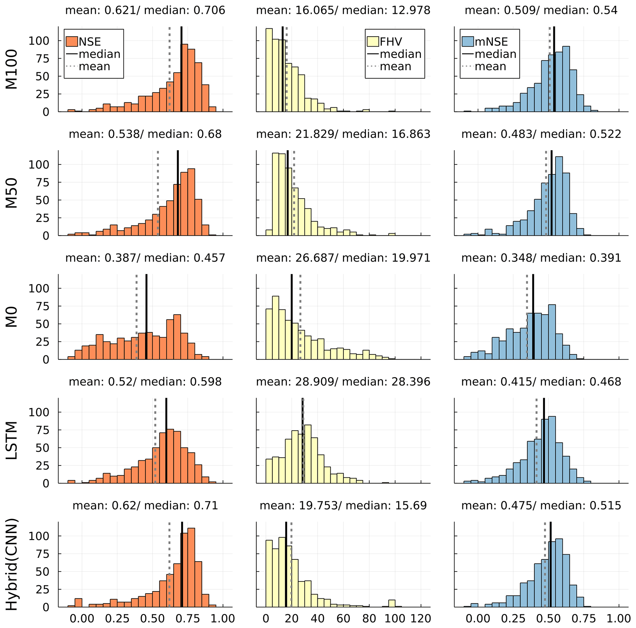
Figure 2Histograms of NSE (orange; optimal value: 1), FHV (yellow; optimal value: 0) and mNSE (blue; optimal value: 1) for the developed neural ODE models M100 and M50, the plain conceptual baseline model M0 and state-of-the-art LSTM and postprocessing hybrid CNN models (bottom; cf. Jiang et al., 2020).
Another special case with α=1 is referred to as the modified coefficient of efficiency (Legates and McCabe Jr, 1999) or, briefly, as mNSE (Jiang et al., 2020). The values of mNSE (CoE1) can be interpreted similarly to NSE (CoE2). The mNSE, however, gives less weight to extreme fluctuations than the NSE, which typically relate to peak flow. Hence, mNSE is better suited to rate low and base flow. Peak flow is rated specifically by the percent bias in the flow duration curve high-segment volume (FHV; Yilmaz et al., 2008):
where Qobs:high and Qsim:high refer to the observed and simulated discharges sorted in descending order, respectively. H defines the number of highest values according to a chosen exceedance probability. Here, for comparability reasons, we use the exceedance probability 0.01 like in Jiang et al. (2020). This means that FHV is based on the highest percent of discharges, as opposed to the typical chosen exceedance probability of 0.02 (Yilmaz et al., 2008). The optimal value of FHV is 0. For comparability and since FHV values can become negative, we use only the absolute values like in Jiang et al. (2020) (where FHV was renamed to absolute peak flow bias, PFAB).
Second, the evaluation of internal model states and processes is conducted in direct comparison between the conceptual model M0 and the neural ODE models M50 and M100: the dynamics of snow and water storages is inspected alongside the model-specific estimated streamflow. Further, the internal processes for discharge, evapotranspiration and melting are isolated and explored over plausible ranges of input variables and model states, for example, discharge as a function of water storage. Additional input variables to the neural networks in M50 and M100 that shall not be explored are kept fixed with catchment-specific values (like mean temperature) as specified in Sect. 4.
Figure 2 shows the distributions of the three evaluation metrics per evaluated model over all 569 considered catchments. NSE, FHV and mNSE are displayed in one row per model, i.e. the two newly developed neural ODE models (M50 and M100), the conceptual model M0 and two state-of-the-art models. The performance values shown for both the hybrid CNN and LSTM model are the original values from Jiang et al. (2020).
For both FHV and mNSE, the M100 scores better in both mean and median than all other models. The distributions over all catchments show clear shifts towards the optimal scores 0 for FHV and 1 for mNSE, respectively. Considering NSE, which is also the calibration metric, M100 outperforms all other models except for the hybrid CNN approach. Yet, both mean and median NSE between the two models do only deviate by a small margin. Looking at the histograms, it can be seen that the hybrid CNN model shows an accumulation of scores slightly above the median for NSE and mNSE and slightly below the median for FHV. Contrarily, the M100 achieves substantially more high scores for NSE and mNSE and lower peak flow errors. At the tails of the histograms, M100 managed to reduce the number of bad results (NSE and mNSE below 0 and FHV around 100 and above).
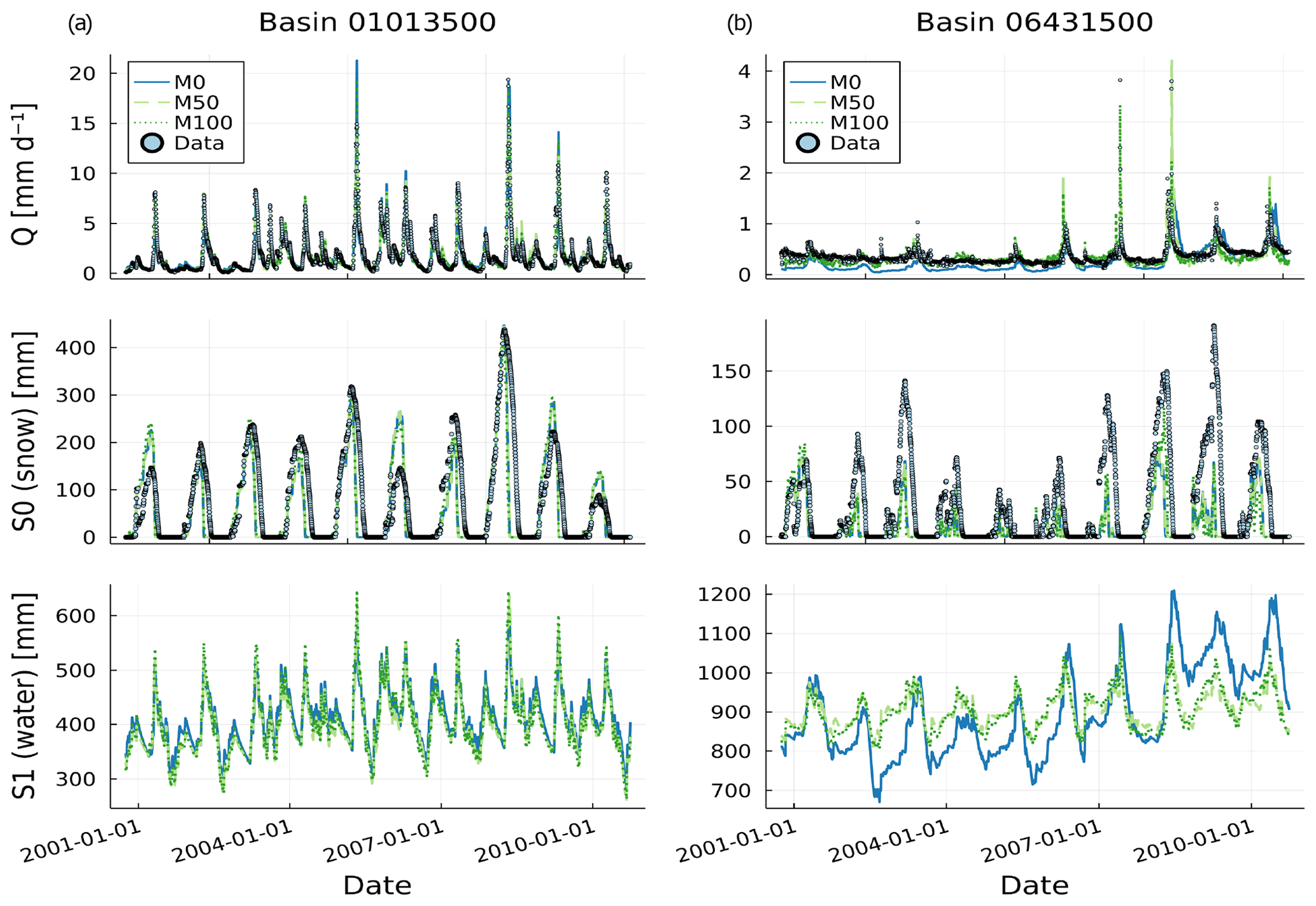
Figure 3Time series of data and model predictions from models M0, M50 and M100 for discharge (top), snow storage (centre) and water storage (bottom; no data) for the test period in basin 1013500 (a) and in basin 6431500 (b).
Considering M50 and M0, the neural ODE model M50 achieves a significant improvement in all metrics over the plain conceptual model: NSE mean and median improve by about 0.15 and 0.23, respectively; mNSE increases in both statistical moments by more than 0.1, while FHV drops by about 25 %. This shows that the conceptual model clearly benefits already from substituting only two processes (ET and Q) by more flexible methods.
It can easily be seen that all models except for model M0 and LSTM achieve performances in a similar range with similar means and medians over all metrics, although the distributions show noticeable differences. While M0 shows better FHV scores with the whole distribution tending toward lower values, the LSTM is considerably better regarding NSE and mNSE. Yet, all distributions for both models deviate clearly from the other models, showing more insufficient values that are low (around 0.0) for NSE and mNSE and high for FHV. This is further discussed in Sect. 5.1, with a special focus on LSTM models.
As with conceptual hydrologic models, the temporal dynamics of processes and states can directly be inspected and analysed in the neural ODE approach. We chose two exemplary basins for demonstration purposes: Fish River near Fort Kent, Maine (ID: 1013500), and Spearfish creek, South Dakota (ID: 6431500). The former one in Maine is a comparably large basin (> 2000 km2) at an average altitude of 250 m, with temperate climate at about 1140 mm annual precipitation and 3.3 ∘C mean temperature. The latter one in South Dakota is a medium-sized (ca. 430 km2), high-altitude basin (average altitude ca. 1890 m) with an annual precipitation of 700 mm and mean temperature of about 5 ∘C. Both basins are covered by forest by slightly more than 90 % and have similar fractions of precipitation that falls as snow of 0.31 and 0.36, respectively.
Figure 3 shows the time series of discharge, snow storage and water storage states from the plain conceptual (M0) and the neural ODE models (M50 and M100) for both basins. For discharge and snow storage, observations are available and are displayed, with the latter being the lumped snow water equivalent (SWE) data. Note that SWE was not used in the calibration.
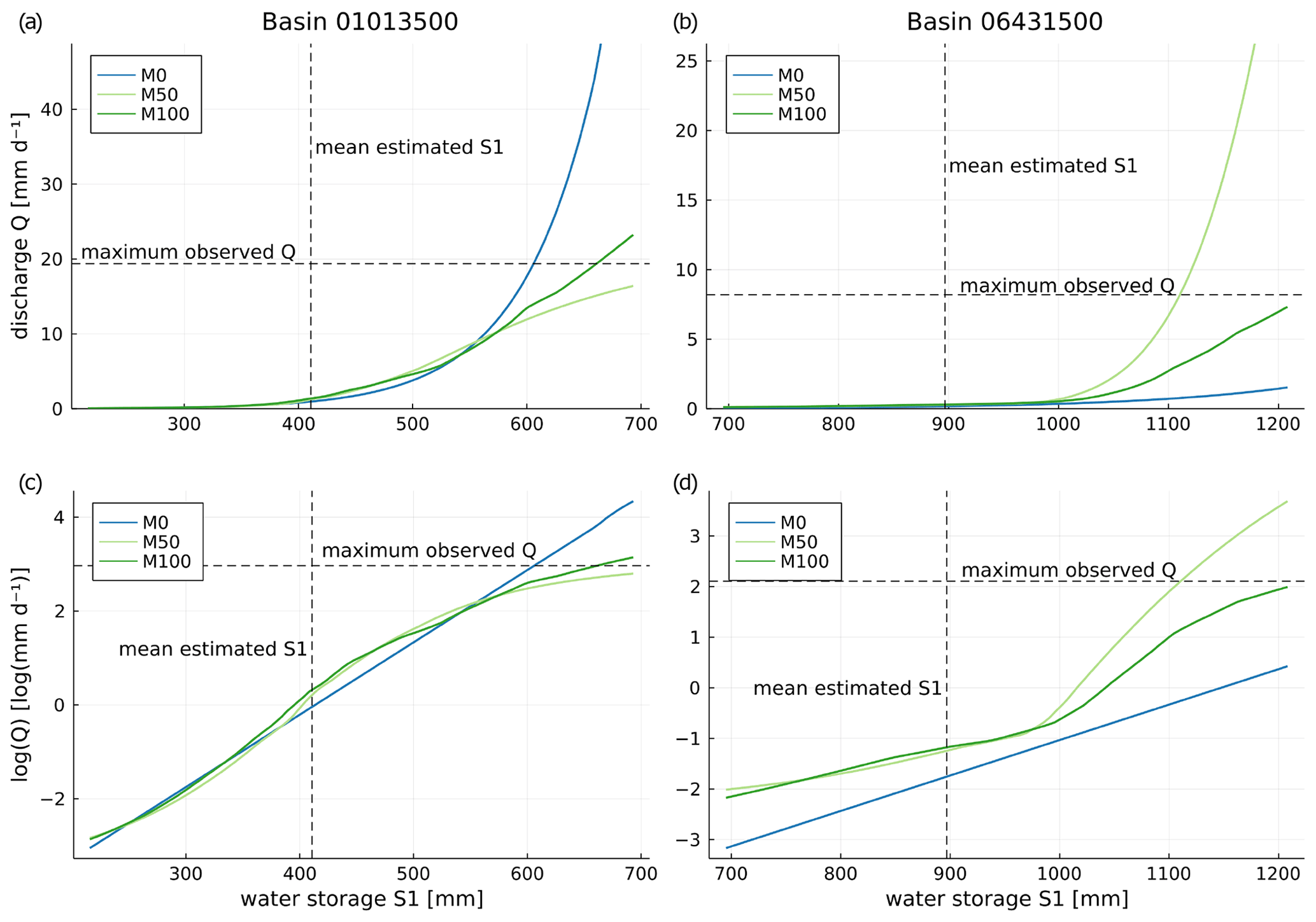
Figure 4Relation between water storage and discharge (a, b) or logarithmic discharge (c, d) in basin 1013500 (left) and basin 6431500 (right) for models M0 (hard-coded relation), M50 and M100 (learned by a neural network, with additional neural network input snow storage fixed at 0 for both M50 and M100 and both precipitation and temperature fixed at basin averages over the training period).
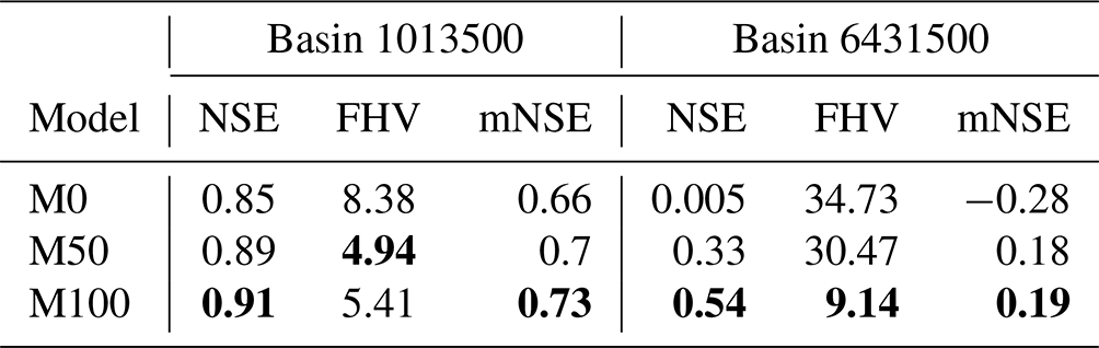
The two basins cover different magnitudes for all depicted variables. For the basin 1013500, model predictions of the three models are very similar. Discharge predictions of all models match observations very well, which is also indicated by overall good metrics in Table 1. The agreement between models is weaker for snow storage, although the general pattern is similar and approximately matches observations. For basin 6431500, model predictions deviate more strongly and show a larger discrepancy to data. As supported by rather bad performance metrics, model M0 underestimates baseflow in large parts and misses both timing and flashiness of peaks.
Table 1Streamflow prediction performance based on NSE (optimum: 1), FHV (optimum: 0) and mNSE (optimum: 1) of the conceptual model (M0) and both neural ODE models (M50 and M100) for basins 1013500 and 6431500. Bold values indicate best performance.
In neither basin do the neural ODE models alter the snow storage component much from the plain conceptual model, although there are small differences in specific years. Overall, the models do catch the temporal pattern of snow accumulation, but there are discrepancies in the magnitude. The models for basin 1013500 show acceptable estimates, while for basin 6431500 they tend to underestimate SWE systematically. At the end of each snow season, the models predict snow to disappear much earlier compared to the observed values for most years. This issue is further discussed in Sect. 5.2. Regarding water storage, there are no data for a direct comparison available. For basin 1013500, all models strongly agree on the dynamics and magnitude of the model state. This is different with model estimates for the second basin 6431500, where the two neural ODEs are similar with only small deviations but both differ strongly from the conceptual model estimate. Apart from variations in the annual cycles, M50 and M100 show much smaller variance, while M0 indicates a general magnitude shift to higher water storage in the last third of the testing period. Together with the significantly better scores in Table 1 of both neural ODE models, this indicates that M0 might not be a suitable choice as model for this particular basin.
Like in plain conceptual models, internal processes like discharge, evapotranspiration and melting can be analysed over plausible ranges of input variables in neural ODE models. Figure 4 shows the relations between water storage S1 and (logarithmic) discharge Q for models M0 (hard-coded, Eq. A5), M50 (learned by ) and M100 (learned by NN100) for both basins. All three discharge–water storage relations appear similar for small to medium water storage values in Fig. 4a and b. Beyond, strong differences evolve: in basin 1013500, the hard-coded relation in M0 shows a strong increase for large values of S1, reaching values much higher than the maximum discharge that was observed over both the training and the testing period. At the same time, M50 shows a linear trend for large water storages, underestimating the maximum observed discharge slightly. For basin 6431500 it is the opposite; M0 underestimates discharge, and model M50 shows a strong tendency to overshoot. In both basins, M100 shows the most plausible relation.
The discrepancies of the learned relations between the three models become even more apparent on the logarithmic scale in Fig. 4c and d. While it is revealed that for basin 1013500 both neural ODE models M50 and M100 estimate higher discharge already for medium storage values, the learned relations flatten toward high storage states. This indicated that the sigmoidal shape prevents the overshooting of discharge in this range as it occurs in M0. For basin 6431500 in Fig. 4d, the learned relations in M50 and M100 even deviate entirely from the simple exponential increase of discharge in M0 that is shown as a straight line on the logarithmic scale. Both neural ODE models generally estimate a higher order of magnitude of the discharge there and also suggest a sigmoidal shape. Generally, both M50 and M100 estimate larger discharge over all storage values than M0. For higher water storage values, M100 learns that discharge grows more than exponentially until it starts flattening again, reaching discharge maxima that are about 2 orders of magnitude higher than those from M0. This pattern is similar for M50 but it overshoots discharge in the high water storage range.

Figure 5Dependence of discharge on precipitation (rain) and water storage for neural ODE models M0, M50 and M100 in basin 1013500 (left; a, c and e, respectively) and in basin 6431500 (right; b, d and f, respectively). For NN100 the additional neural network input snow storage was fixed at 0 in both basins, and temperature was fixed at the average temperatures over the training period (3.3 ∘C for basin 1013500 and 5 ∘C for basin 6431500).
Exceeding plain conceptual models, the neural ODE approach further allows us to directly analyse the (cross-)impact of additionally assigned variables to specific processes. Both neural networks and NN100 in M50 and M100, respectively, also use precipitation as input. Figure 5 depicts the relations of discharge to water storage and precipitation for the three models in each basin. Note that the magnitudes of discharge vary between basins and that discharge in the conceptual model M0 depends only on water storage. For model M0, the very high discharge predictions in basin 1013500 and the very low ones in basin 6431500 are clearly shown in Fig. 5a and b, respectively.
For basin 1013500, models M50 and M100 show an overall similar pattern in Fig. 5c and e, respectively, with M100 reaching higher magnitudes. Both models locate the highest discharge in the same region of high water storage and medium to low precipitation. For very small precipitation at high water storage M100 in particular indicates a slight decline in discharge. Interestingly, neither model shows an increase of discharge with stronger precipitation. The decline in discharge could be related to the lower frequency of strong rain events in the basin and the resulting detriment of the neural networks to learn another relation. Hence, it might be subject to higher uncertainty in this variable range. This is further discussed in Sect. 5.2.
The expected trend of increasing discharge for increasing rain is clearly visible for both models in basin 6431500 (Fig. 5d and f). Notably, a peak in discharge for high water storage and small rain rates is visible, similar to the other basin. Investigations about whether this could be an indication of a general non-linearity require further discussion (see Sect. 5.2).
Figure 6 depicts the models' dependences of the evapotranspiration terms (without Lday) on temperature and water storage. Note that the magnitude ranges of evapotranspiration indicated by colours are the same between the basins. The hard-coded relation according to Hamon's formula in the conceptual model M0 shows the most regular behaviour in Fig. 6a and b for both catchments: for temperatures below 0 ∘C, there is very small to no evapotranspiration. Overall, increasing temperatures or water storages are associated with increasing evapotranspiration, although the general magnitude is smaller for basin 6431500.
For basin 1013500, M0 shows much higher ET estimates over a large range of temperature–water storage combinations compared to the other two models. M50 only reaches maximal ET in the region of medium to high water storage and very high temperatures (extreme to unrealistic for the considered basin) as shown in Fig. 6c. The general trend of higher ET for higher temperature is also learned by the , but the pattern is not as regular as in M0. In particular, for water storage values at the extremes, a decrease of evapotranspiration is assumed. This indicates that either the water storage–ET relation is not as proportional in these regions as assumed by Hamon's formula, or there are a lack of data points covering these ranges, making it challenging for to elicit the underlying relation. Nonetheless, the elicited relation appears plausible, in particular for small water storage.
In contrast to M50, M100 shows a much more regular dependence of ET on temperature and water storage, as shown in Fig. 6e. It shows the same regular increase of ET with temperature as in M0 but a smaller dependence on water storage. Yet, the magnitude of ET estimated by the neural network in M100 is generally smaller. Hence, according to M100, evapotranspiration plays an overall smaller role in the water balance than represented in the conceptual model M0.
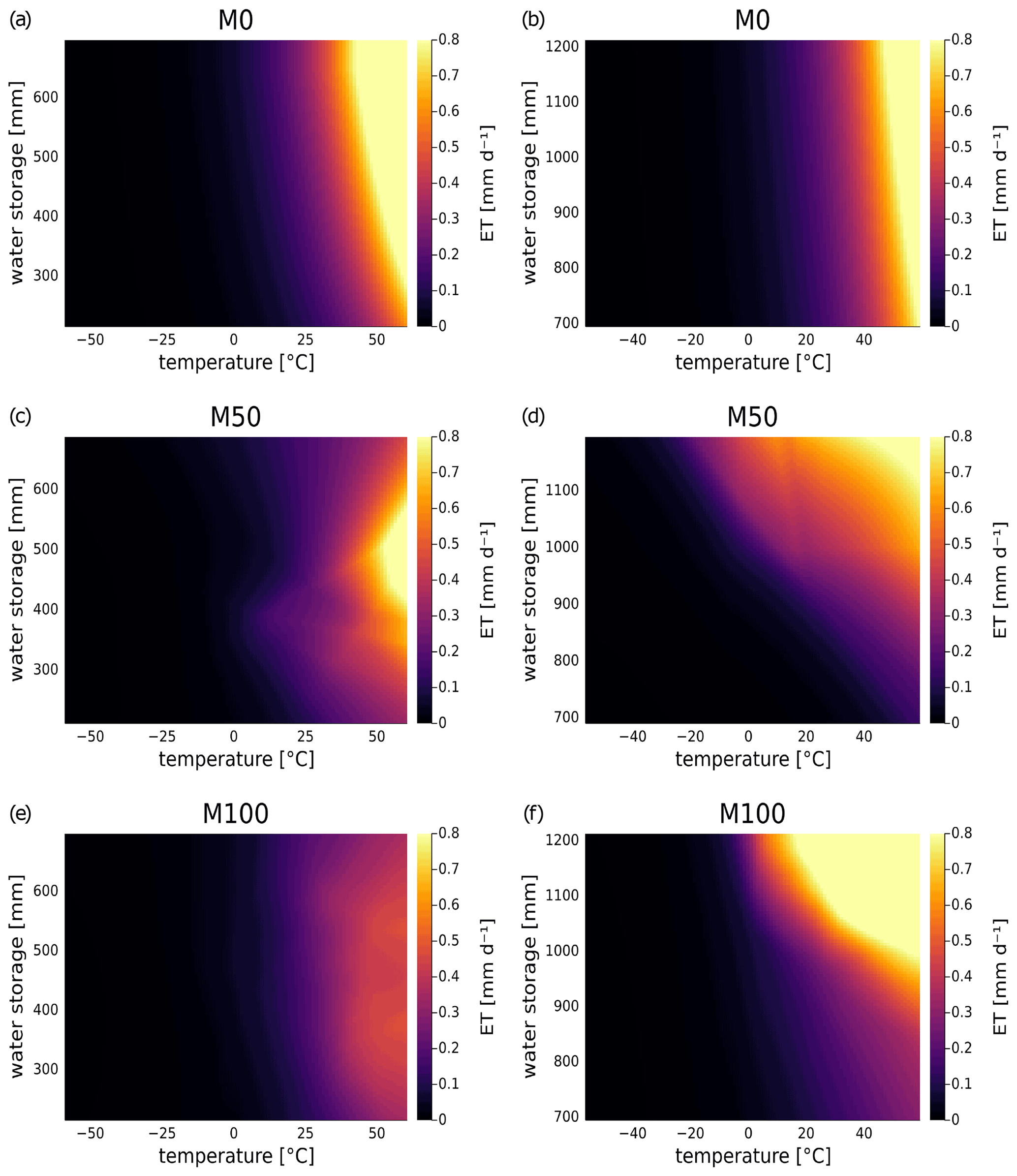
Figure 6Dependence of evapotranspiration on temperature and water storage for neural ODE models M0, M50 and M100 in basin 1013500 (left; a, c and e, respectively) and in basin 6431500 (right; b, d and f, respectively). For and NN100, the additional neural network input snow storage was fixed at 0 in both basins, and precipitation for NN100 was fixed at the average over the training period (3 mm d−1 for basin 1013500 and 1.9 mm d−1 for basin 6431500).
In basin 6431500, both models show a much more similar pattern for the maxima of evapotranspiration (Fig. 6d and f) although M100 indicates a much stronger increase in magnitude for rising temperatures and water storage. In contrast to Hamon's formula in M0, the neural networks do not allocate strong ET rates to small to medium water storages even for higher temperatures, but both models depict higher rates even for lower temperatures if water storage is high.
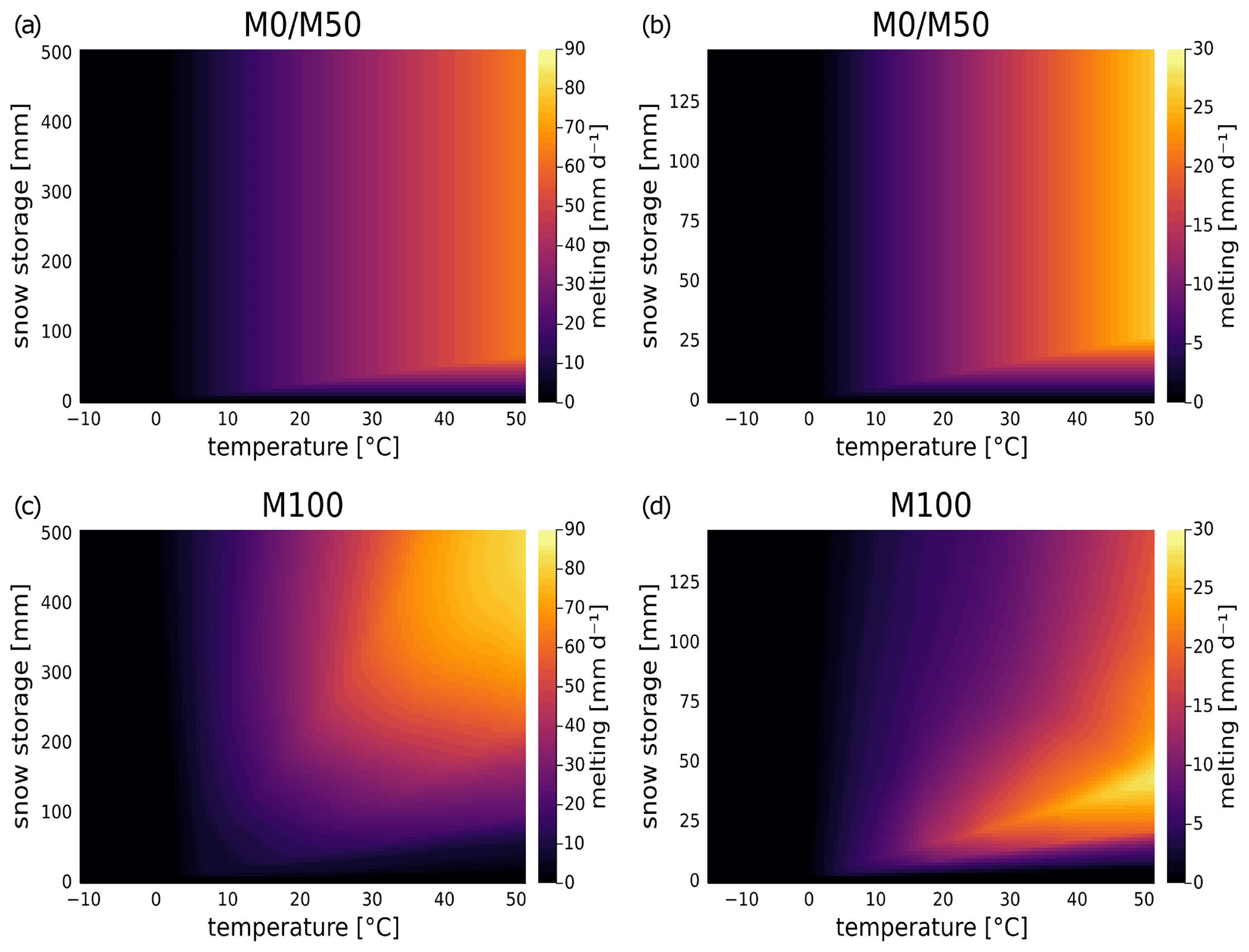
Figure 7Dependence of melting rate on temperature and snow storage for neural ODE models M0/M50 and M100 in basin 1013500 (left; a and c, respectively) and in basin 6431500 (right; b and d, respectively). For NN100, the additional neural network inputs were fixed at basin averages of water storage and precipitation (3 mm d−1 for basin 1013500 and 1.9 mm d−1 for basin 6431500) over the training period.
The effect of snow storage and temperature on melting rates is displayed in Fig. 7. M0 and M50 employ the same hard-coded melting formula (see Eq. A4), while in M100, the relation is learned by NN100. Note that the range of magnitudes of melting rates and snow storage is much higher in basin 1013500 than in basin 6431500. Despite some differences, there are also general trends over all models and both basins: plausibly, no relation shows snowmelt for temperatures below 0 ∘C – this is determined for M50 and M0 but also not altered in M100. For larger temperatures, melting rates constantly increase. The only exception is very small snow storage values where no to only slowly growing melting occurs in the models.
For M100, differences between the basins and from the hard-coded melting linear relationship in M0/M50 are clearly observable: for basin 1013500 (Fig. 7c) M100 shows the smoothest increase in the direction of higher temperatures and higher snow storage and also reaches considerably higher magnitudes. Yet, with small but growing snow storage for higher temperatures, M0/M50 shows a stronger increase over a smaller range. This increase is similar for M100 in basin 6431500 (Fig. 7d), although for higher snow storage, there is a decline in melting rate over the entire range for temperatures above 15 ∘C. Further discussed in Sect. 5.2, this could again be due to a lack of training points in a catchment of warmer climate.
Of course, the highest temperatures covered in the above analysis are unrealistic to be associated with snow cover. Elevation information that would make it possible to consider snow cover in high altitudes while already having warm temperatures in lower parts of the catchment is neglected. Nonetheless, we demonstrate that a physical extrapolation and analysis of individual processes is possible with the neural ODE approach, just as is traditionally done with conceptual models.
5.1 Benchmarking
All four machine-learning-based hydrologic models show a significant improvement over the plain conceptual hydrologic model M0. Results indicate that more information from training data can be leveraged by partial or pure data-driven models, and considerably higher rating scores are achieved. Arguably, the EXP-Hydro is a very simplistic bucket model, and more sophisticated conceptual hydrologic models exist that achieve higher scores (see SAC-SMA (Sacramento Soil Moisture Accounting Model) in Appendix A3). Yet, more complex conceptual hydrologic models also require more tailored model features and higher parameterizations that again entail more assumptions and fine-tuning.
Note that the displayed results for LSTM are the original values from Jiang et al. (2020). There, they were obtained by catchment-specific calibration and validation. However, over recent years, LSTM models have achieved much higher scores when being calibrated to many catchments simultaneously while also including static catchment attributes (like topography and climatic indices, etc.) as additional inputs to the model (Kratzert et al., 2019c; Feng et al., 2020). LSTM models have demonstrated their ability to transfer learned relations between input variables, attributes and streamflow to unseen catchments, often yielding highly accurate predictions. This application case of large-sample hydrology is however different from the application scenario here.
Despite their success, machine-learning models in hydrology like LSTMs are known for often underestimating high flow events (Kratzert et al., 2018). They often miss sharp peaks as they regularly occur in hydrographs. Conceptual models with their hard-coded peak flow relations are typically very good at this task. Both neural ODE models – and especially M100 – show a clear improvement in this respect based on learned relations that do not have to use a threshold to distinguish between base and peak flow. FHV scores of M50 are similar (yet still higher) to the hybrid CNN model that already showed an improvement in peak flow prediction, taking conceptual model predictions as additional model input (see Jiang et al., 2020). M100 achieves an even higher level of performance, with a median of about 13 and a mean of about 16. The improved base flow prediction performance is likewise indicated by the highest mNSE scores (median 0.54 and mean 0.51). Overall, we summarize that neural ODE models perform similarly well as or better than alternative state-of-the art partial or pure machine-learning models.
5.2 Internal states and processes
The overall better performance of neural ODE models compared to plain conceptual models is associated with decisive differences in the model internal dynamics and process relations. Results demonstrate that the pre-training of neural networks in order to mimic hard-coded processes before the full neural ODE training does not prevent the neural networks from learning new and vastly different relations. With neural ODEs being built on the same conceptual model structure, individual states and processes can easily be analysed and compared between different models, or they can be investigated over specific ranges of input variables and model states. Ultimately, the dependencies learnt by the neural networks might help to develop more sophisticated relations for discharge and other processes.
In the variable ranges where many data were available, the neural ODE models elicited plausible relations for the investigated processes. Yet, the analyses indicated that in the extreme ranges of the process-dependent variables learned, relations might be counter-intuitive or subject to uncertainty. This is partially caused by a lack of data: 20 years of training data for a single catchment typically does not provide enough information to certainly extrapolate towards these limits. Although general process trends often appeared to be plausible, cases remain that are hardly explainable (e.g. a decrease of melting rate for growing snow storage). More data might help to refine functional relations for broader data ranges to a higher level of accuracy and to turn parts of the extrapolation into an interpolation problem. Yet, this will only be one part of the solution since further extrapolation is always a challenging task – especially for purely data-driven methods. Here, we conjecture that the hybrid neural ODE models benefit from their physical structure that enforces regularization. It informs the model parameters aside of data during training and naturally constrains predictions during interpolation and extrapolation tasks – just like the modelled natural system at hand being constrained by physical limits. We think that this combination of more data and physical structure might help neural ODE models to elicit reliable functional relations that can then be evaluated in plausibility testing. An example for this could be a centennial rainfall-runoff event that might not be covered by our data, but we would still be able to qualitatively judge whether the extrapolated relation to predict it is plausible or not.
None of the models were trained on snow water equivalent data, but due to their conceptual structure M0/M50 and M100 learned snow dynamics indirectly via the snow storage state of the model. Despite the close agreement regarding their predictions of snow in both considered basins, all models depict limitations of the lumped snow storage approach: melting of snow is often predicted earlier than shown for the catchment by data (see Fig. 3). In higher altitudes, snow stays much longer, and new precipitation might also fill the snow storage there, even if spring and summer might already have started in lower altitudes. Using only lumped driving forces like average temperature as input variables to the model prohibits the models from accounting for these effects and leads to potentially inaccurate estimates. Since the CAMELS dataset provides elevation-band data for snow water equivalent, we assume that including elevation-resolved snow storage units in the neural ODE models might improve this. Generally, a lumped model structure with only a few processes and states facilitates information from data being taken up falsely by parameters, even though it should be encoded in other parts of the model. This might additionally exacerbate the elicitation of clear relations. As a remedy, a more detailed conceptual structure might improve the encoding of underlying functional relations.
Hydrologic neural ODE models fuse the modular bucket-type structure of conceptual hydrologic models with machine learning. Plainly spoken, neural ODE models are conceptual hydrologic models with deep learning cores. The presented models M50 and M100 depict hydrologic implementations of the general neural ODE approach (Chen et al., 2018; Rackauckas et al., 2020) – and to our knowledge the first ones in hydrology. The substitution of constitutive functions by neural networks has shown to significantly increase predictive performance compared to a plain conceptual model while keeping the same natural physical constraints. Overall, hydrologic neural ODE models perform similarly well as or better than state-of-the-art pure or partial machine-learning models but overcome three different limitations of former approaches as introduced in Sect. 1:
-
First, using the conceptual hydrologic model structure preserves the interpretability of the model as traditionally given by conceptual models and appreciated by the hydrologic community. Internal model states and processes can directly be inspected for plausibility, and their physical interpretation fosters system understanding. The neural ODE approach might further trigger advancement in a more fundamental manner of building “conceptual” models: theoretically, modellers only need to set up the conceptual framework but do not have to specify parameterizations within the model and let the neural networks learn plausible relations. Potentially, even features that are often neglected in typical conceptual models, like hysteresis (Gharari and Razavi, 2018), could be elicited.
-
Second, the neural ODE allows for physically constrained, continuous time solutions. In principle, this also allows us to include data at an irregular temporal resolution for both training and testing. Physical principles and mechanistic structure act as guide rails that are naturally included and do not have to be learned or enforced as with pure machine-learning approaches. The physical constraints act as regularization that bound variability of the model. At the same time, the method is flexible enough to learn constitutive relations from data.
-
Third, our approach invites prior physical knowledge to be incorporated into the model. For instance, the neural ODE approach allows us to include processes that are fully known as hard-coded features, like a sewage treatment plant discharging into the stream at a known temporal pattern. Locally, expert knowledge might be available about hydrologic systems that can be accounted for. Pure data-driven methods might not be able to infer this knowledge from data alone, and pure mechanistic models might not provide the desired flexibility like neural ODE models.
In principle, the introduced approach can be applied to any conceptual hydrologic model. Numerous alternative bucket-type models and frameworks exist that can be fused with neural networks partially or entirely. The number of states and processes is adjustable according to specific requirements of the modelling problem at hand or in a more generic setup for multiple catchments. Already the EXP-Hydro model used as a rather simplistic example of conceptual model facilitated a drastic improvement of model performance when used as a basis for neural ODE models. Many sophisticated conceptual models exist (like SAC-SMA) that could also serve as a framework for more sophisticated hydrologic neural ODE models.
With the hydrological neural ODE model, we seek to introduce a tool in between existing top-down and bottom-up approaches that paves the way for various subsequent research routes. For example, the deterministic model can be made probabilistic to enable uncertainty assessments as currently performed for stochastic hydrologic models (Reichert et al., 2021). Also, due to its generic setup, the neural ODE approach appears to be suitable for being trained with multiple basins simultaneously, including static attributes like in respective investigations for LSTM models (Kratzert et al., 2019c; Feng et al., 2020; Jiang et al., 2020). This large-sample hydrology setting might be particularly useful to further investigate process relations in data-scarce variable ranges. We will investigate this in a subsequent step.
A1 EXP-Hydro equations
The simple rainfall-runoff model EXP-Hydro (Patil and Stieglitz, 2014) comprises only two state variables representing buckets, five mechanistic processes and six parameters Θ (see Table A1). There are three inputs to the model: length of day Lday, temperature T and precipitation P.
Table A1EXP-hydro parameter definitions, meaning and units (cf. Patil and Stieglitz, 2014).

For ease of readability and comparability to Jiang et al. (2020), parameters are written in Table A1 as they were originally defined by Patil and Stieglitz (2014). Further, the storage state Ssnow is written as S0, and Swater is written as S1. For ease of readability, dependence on time is implicitly assumed, and t is dropped. Moreover, the driving forces and model states relevant for each process are explicitly named. Hence, the processes in EXP-Hydro are formulated as follows.
A2 Rationale behind M50 and M100
With the substitutions from M0 to M50, we want to highlight two important features of the neural ODE modelling approach. First, physical knowledge can directly be included in the model: the ET prescription uses potential evapotranspiration based on Hamon's formula (Hamon, 1963), in which length of day Lday is factored (see Appendix A1). This is a fully accessible input variable to the model – for a certain latitude and time, it is physically fixed information (that theoretically could also be calculated within the model). When used in a multiplication as in the chosen ET prescription, it can therefore simply be kept as a factor, and only the rest of the ET formula has to be substituted and learned by a neural network. It is a plausible assumption that ET is proportional to the length of day, as represented in the mechanistic description of Hamon's formula, referring to the light activation of plants' stomata. This proportionality is therefore kept in M50 when substituting the rest of the ET formula by a neural network. As can be seen in the model scheme in Fig. 1a, the NNET does not obtain Lday as input but instead Ssnow as there could be interference of snow cover with evapotranspiration.
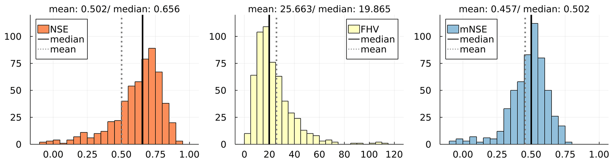
Figure A1Histograms of NSE (orange; optimal value: 1), FHV (yellow; optimal value: 0) and mNSE (blue; optimal value: 1) for the SAC-SMA model over 569 basins.
Second, in hydrologic models, discharge is often split up into (at least) a base flow component and an excess or peak flow component that acts above a certain threshold of the water storage. In the neural ODE approach, these two flow components can be substituted by a neural network with a single output node because neural networks are particularly suited to learn nonlinearities. Hence, rather than defining an “artificial” threshold beyond which a new process is added, NNs can learn a continuous relation between water storage and model inputs to discharge. Unlike the Q formula in M0, we added precipitation as a second input to the NNQ in M50 to potentially account for direct runoff.
M50 is meant to demonstrate how strongly predictive performance can be increased by including some more flexible, data-driven model parts, i.e. only partial modifications within the traditional modelling approach. This approach is similar to the one in Bennett and Nijssen (2021), although there, fixed time stepping was applied, only one internal process was substituted and exactly the same inputs were given to the NN as were given to the mechanistic process. Further, their goal was not to ultimately enhance stream flow prediction but to substitute the internal process, i.e. the turbulent heat flux.
In the next step from M50 to M100, the other mechanistic processes that are “hard-coded” in the plain EXP-Hydro are also substituted. These are to distinguish between precipitation as rain or snow and the melting process that transfers water from the snow storage unit to the main storage unit. As opposed to ET and Q, over certain parts of the year, these processes do not occur; for example, if all snow was molten in spring, there is no melting process going on in summer. Hence the neural ODE model has to learn these regime differences. Again, Lday is factored out in the ET process, which highlights a feature of the neural ODE approach: if Lday shall be included, it could also be given to the NN as input. Yet, the NN could also learn a relation between Lday and Q which is physically implausible. In a plain machine-learning approach, this specific use of Lday cannot be as easily assigned.
A3 SAC-SMA
The current benchmark hydrologic model for the CAMELS US dataset is the Sacramento Soil Moisture Accounting Model (SAC-SMA; see Newman et al., 2015, and references therein). The simulated discharge values from the SAC-SMA model used for evaluation are taken from the CAMELS dataset (Addor et al., 2017) (discharge predictions for the test period 1 October 2000–30 September 2010).
Note, however, that training and testing periods for the SAC-SMA were different from those used here. The SAC-SMA was calibrated with a split-sample approach, where 30 years of data (1 October 1980 to 30 September 2010) was split up into two parts, each covering 15 years. For details, refer to Newman et al. (2015). In contrast, we used the first 20 years for training and the last 10 years for testing. The scores of NSE, FHV and mNSE for the SAC-SMA model shown in Fig. A1 are evaluated for this 10-year testing period. Hence, the results should only be considered an indication and not a strict assessment when being directly compared to the results in Sect. 3.
Figure A1 shows the overall performance of the SAC-SMA model on all the 569 basins for the testing period. It is significantly better than the simple conceptual EXP-Hydro model implemented as M0, and it achieves comparable levels of performance compared to the partial and pure machine-learning models evaluated (see Sect. 3). Yet, it does not score better than these, although many more processes and interrelations (and corresponding assumptions) were put into the model: 20 of in total 35 parameters were calibrated and the rest adjusted according to expert knowledge (Newman et al., 2015). This demonstrates that, in principle, conceptual models do have the ability to reach high scores in model rating – but come with comparably high effort in setup, tuning and adjustment compared to pure or hybrid machine-learning-based methods.
All software was written in the programming language Julia (https://julialang.org/; Julia, 2022). The code is available at https://github.com/marv-in/HydroNODE (Höge, 2022a) and citable via https://doi.org/10.5281/zenodo.7085028 (Höge, 2022b).
MH had the original idea and developed the conceptualization and methodology of the study. MH developed the software with initial support by AS. MH conducted all model simulations and their formal analysis. Results were discussed and further research steps planned between CA, MBJ, AS, FF and MH. The visualizations and the original draft of the manuscript were prepared by MH, and reviewing and editing were provided by MBJ, CA, AS and FF. Funding was acquired by FF. All authors have read and agreed to the current version of the paper.
At least one of the (co-)authors is a member of the editorial board of Hydrology and Earth System Sciences. The peer-review process was guided by an independent editor, and the authors also have no other competing interests to declare.
Publisher's note: Copernicus Publications remains neutral with regard to jurisdictional claims in published maps and institutional affiliations.
The authors would like to thank Shijie Jiang for providing the original results from Jiang et al. (2020) for the model benchmarking in this work. We thank Peter Reichert for fruitful discussions and suggestions that helped improve the manuscript. Further, we thank Andreas Wunsch, Miyuru Gunathilake and Juan Pablo Carbajal for valuable comments and suggestions during the review and interactive discussion.
This paper was edited by Marnik Vanclooster and reviewed by Miyuru Gunathilake and Andreas Wunsch.
Abbott, M., Bathurst, J., Cunge, J., O'Connell, P., and Rasmussen, J.: An introduction to the European Hydrological System – Systeme Hydrologique Europeen, “SHE”, 1: History and philosophy of a physically-based, distributed modelling system, J Hydrol., 87, 45–59, https://doi.org/10.1016/0022-1694(86)90114-9, 1986. a
Addor, N., Newman, A. J., Mizukami, N., and Clark, M. P.: The CAMELS data set: catchment attributes and meteorology for large-sample studies, Hydrol. Earth Syst. Sci., 21, 5293–5313, https://doi.org/10.5194/hess-21-5293-2017, 2017. a, b
Bennett, A. and Nijssen, B.: Deep learned process parameterizations provide better representations of turbulent heat fluxes in hydrologic models, Water Resour. Res., 57, e2020WR029328, https://doi.org/10.1029/2020WR029328, 2021. a, b
Bezanson, J., Edelman, A., Karpinski, S., and Shah, V. B.: Julia: A fresh approach to numerical computing, SIAM Rev., 59, 65–98, 2017. a
Chen, R. T., Rubanova, Y., Bettencourt, J., and Duvenaud, D.: Neural ordinary differential equations, arXiv [preprint], arXiv:1806.07366, 2018. a, b
Clark, M. P., Slater, A. G., Rupp, D. E., Woods, R. A., Vrugt, J. A., Gupta, H. V., Wagener, T., and Hay, L. E.: Framework for Understanding Structural Errors (FUSE): A modular framework to diagnose differences between hydrological models, Water Resour. Res., 44, W00B02, https://doi.org/10.1029/2007WR006735, 2008. a
Clark, M. P., Nijssen, B., Lundquist, J. D., Kavetski, D., Rupp, D. E., Woods, R. A., Freer, J. E., Gutmann, E. D., Wood, A. W., Brekke, L. D., Arnold, J. R., Gochis, D. J., and Rasmussen, R. M.: A unified approach for process-based hydrologic modeling: 1. Modeling concept, Water Resour. Res., 51, 2498–2514, 2015. a
Feng, D., Fang, K., and Shen, C.: Enhancing streamflow forecast and extracting insights using long-short term memory networks with data integration at continental scales, Water Resour. Res., 56, e2019WR026793, https://doi.org/10.1029/2019WR026793, 2020. a, b, c
Fenicia, F., Savenije, H. H., Matgen, P., and Pfister, L.: Understanding catchment behavior through stepwise model concept improvement, Water Resour. Res., 44, W01402, https://doi.org/10.1029/2006WR005563, 2008. a
Fenicia, F., Kavetski, D., and Savenije, H. H.: Elements of a flexible approach for conceptual hydrological modeling: 1. Motivation and theoretical development, Water Resour. Res., 47, W11510, https://doi.org/10.1029/2010WR010174, 2011. a, b
Fenicia, F., Kavetski, D., Savenije, H. H., Clark, M. P., Schoups, G., Pfister, L., and Freer, J.: Catchment properties, function, and conceptual model representation: is there a correspondence?, Hydrol. Process., 28, 2451–2467, 2014. a
Fenicia, F., Kavetski, D., Savenije, H. H., and Pfister, L.: From spatially variable streamflow to distributed hydrological models: Analysis of key modeling decisions, Water Resour. Res., 52, 954–989, 2016. a
Frame, J. M., Kratzert, F., Klotz, D., Gauch, M., Shalev, G., Gilon, O., Qualls, L. M., Gupta, H. V., and Nearing, G. S.: Deep learning rainfall–runoff predictions of extreme events, Hydrol. Earth Syst. Sci., 26, 3377–3392, https://doi.org/10.5194/hess-26-3377-2022, 2022. a, b
Gauch, M., Kratzert, F., Klotz, D., Nearing, G., Lin, J., and Hochreiter, S.: Rainfall–runoff prediction at multiple timescales with a single Long Short-Term Memory network, Hydrol. Earth Syst. Sci., 25, 2045–2062, https://doi.org/10.5194/hess-25-2045-2021, 2021. a
Gharari, S. and Razavi, S.: A review and synthesis of hysteresis in hydrology and hydrological modeling: Memory, path-dependency, or missing physics?, J. Hydrol., 566, 500–519, 2018. a
Gharari, S., Gupta, H. V., Clark, M. P., Hrachowitz, M., Fenicia, F., Matgen, P., and Savenije, H. H. G.: Understanding the Information Content in the Hierarchy of Model Development Decisions: Learning From Data, Water Resour. Res., 57, e2020WR027948, https://doi.org/10.1029/2020WR027948, 2021. a, b, c
Gnann, S. J., McMillan, H. K., Woods, R. A., and Howden, N. J.: Including regional knowledge improves baseflow signature predictions in large sample hydrology, Water Resour. Res., 57, e2020WR028354, https://doi.org/10.1029/2020WR028354, 2021. a
Hamon, W. R.: Computation of direct runoff amounts from storm rainfall, Vol. 63, International Association of Scientific Hydrology Publication, 52–62, https://iahs.info/uploads/dms/063006.pdf (last access: 11 October 2022), 1963. a, b
Hoedt, P.-J., Kratzert, F., Klotz, D., Halmich, C., Holzleitner, M., Nearing, G., Hochreiter, S., and Klambauer, G.: MC-LSTM: Mass-Conserving LSTM, arXiv [preprint], arXiv:2101.05186, 2021. a
Höge, M.: HydroNODE, GitHub [code], https://github.com/marv-in/HydroNODE (last access: 21 August 2022), 2022a. a
Höge, M.: HydroNODE-v1.0.0, Zenodo [code], https://doi.org/10.5281/zenodo.7085028, 2022b. a
Höge, M., Wöhling, T., and Nowak, W.: A primer for model selection: The decisive role of model complexity, Water Resour. Res., 54, 1688–1715, 2018. a
Holzinger, A.: Interactive machine learning for health informatics: when do we need the human-in-the-loop?, Brain Informatics, 3, 119–131, 2016. a
Innes, M., Edelman, A., Fischer, K., Rackauckas, C., Saba, E., Shah, V. B., and Tebbutt, W.: A differentiable programming system to bridge machine learning and scientific computing, arXiv [preprint], arXiv:1907.07587, 2019. a
Jiang, S., Zheng, Y., and Solomatine, D.: Improving AI system awareness of geoscience knowledge: symbiotic integration of physical approaches and deep learning, Geophys. Res. Lett., 47, e2020GL088229, https://doi.org/10.1029/2020GL088229, 2020. a, b, c, d, e, f, g, h, i, j, k, l, m, n, o, p, q
Julia: The Julia Programming Language, https://julialang.org/, last access: 11 October 2022. a
Karniadakis, G. E., Kevrekidis, I. G., Lu, L., Perdikaris, P., Wang, S., and Yang, L.: Physics-informed machine learning, Nature Reviews Physics, 3, 422–440, 2021. a
Karpatne, A., Atluri, G., Faghmous, J. H., Steinbach, M., Banerjee, A., Ganguly, A., Shekhar, S., Samatova, N., and Kumar, V.: Theory-guided data science: A new paradigm for scientific discovery from data, IEEE T Knowl. Data En., 29, 2318–2331, 2017. a
Kirchner, J. W.: Getting the right answers for the right reasons: Linking measurements, analyses, and models to advance the science of hydrology, Water Resour. Res., 42, W03S04, https://doi.org/10.1029/2005WR004362, 2006. a
Kirchner, J. W.: Catchments as simple dynamical systems: Catchment characterization, rainfall-runoff modeling, and doing hydrology backward, Water Resour. Res., 45, W02429, https://doi.org/10.1029/2008WR006912, 2009. a
Knoben, W. J., Freer, J. E., Peel, M., Fowler, K., and Woods, R. A.: A brief analysis of conceptual model structure uncertainty using 36 models and 559 catchments, Water Resour. Res., 56, e2019WR025975, https://doi.org/10.1029/2019WR025975, 2020. a, b
Kraft, B., Jung, M., Körner, M., Koirala, S., and Reichstein, M.: Towards hybrid modeling of the global hydrological cycle, Hydrol. Earth Syst. Sci., 26, 1579–1614, https://doi.org/10.5194/hess-26-1579-2022, 2022. a
Kratzert, F., Klotz, D., Brenner, C., Schulz, K., and Herrnegger, M.: Rainfall–runoff modelling using Long Short-Term Memory (LSTM) networks, Hydrol. Earth Syst. Sci., 22, 6005–6022, https://doi.org/10.5194/hess-22-6005-2018, 2018. a, b, c
Kratzert, F., Herrnegger, M., Klotz, D., Hochreiter, S., and Klambauer, G.: NeuralHydrology–interpreting LSTMs in hydrology, in: Explainable AI: Interpreting, explaining and visualizing deep learning, edited by: Samek, W., Montavon, G., Vedaldi, A., Hansen, L., and Müller, K. R., Springer, 347–362, https://doi.org/10.1007/978-3-030-28954-6_19, 2019a. a
Kratzert, F., Klotz, D., Herrnegger, M., Sampson, A. K., Hochreiter, S., and Nearing, G. S.: Toward improved predictions in ungauged basins: Exploiting the power of machine learning, Water Resour. Res., 55, 11344–11354, 2019b. a, b
Kratzert, F., Klotz, D., Shalev, G., Klambauer, G., Hochreiter, S., and Nearing, G.: Towards learning universal, regional, and local hydrological behaviors via machine learning applied to large-sample datasets, Hydrol. Earth Syst. Sci., 23, 5089–5110, https://doi.org/10.5194/hess-23-5089-2019, 2019c. a, b, c
Kratzert, F., Klotz, D., Hochreiter, S., and Nearing, G. S.: A note on leveraging synergy in multiple meteorological data sets with deep learning for rainfall–runoff modeling, Hydrol. Earth Syst. Sci., 25, 2685–2703, https://doi.org/10.5194/hess-25-2685-2021, 2021. a
Lechner, M. and Hasani, R.: Learning long-term dependencies in irregularly-sampled time series, arXiv [preprint], arXiv:2006.04418, 2020. a
Lees, T., Buechel, M., Anderson, B., Slater, L., Reece, S., Coxon, G., and Dadson, S. J.: Benchmarking data-driven rainfall–runoff models in Great Britain: a comparison of long short-term memory (LSTM)-based models with four lumped conceptual models, Hydrol. Earth Syst. Sci., 25, 5517–5534, https://doi.org/10.5194/hess-25-5517-2021, 2021. a
Lees, T., Reece, S., Kratzert, F., Klotz, D., Gauch, M., De Bruijn, J., Kumar Sahu, R., Greve, P., Slater, L., and Dadson, S. J.: Hydrological concept formation inside long short-term memory (LSTM) networks, Hydrol. Earth Syst. Sci., 26, 3079–3101, https://doi.org/10.5194/hess-26-3079-2022, 2022. a, b
Legates, D. R. and McCabe Jr, G. J.: Evaluating the use of “goodness-of-fit” measures in hydrologic and hydroclimatic model validation, Water Resour. Res., 35, 233–241, 1999. a, b
Li, L., Sullivan, P. L., Benettin, P., Cirpka, O. A., Bishop, K., Brantley, S. L., Knapp, J. L., van Meerveld, I., Rinaldo, A., Seibert, J., Wen, H., and Kirchner, J. W.: Toward catchment hydro-biogeochemical theories, Wiley Interdisciplinary Reviews: Water, 8, e1495, https://doi.org/10.1002/wat2.1495, 2021. a
Loritz, R., Gupta, H., Jackisch, C., Westhoff, M., Kleidon, A., Ehret, U., and Zehe, E.: On the dynamic nature of hydrological similarity, Hydrol. Earth Syst. Sci., 22, 3663–3684, https://doi.org/10.5194/hess-22-3663-2018, 2018. a
Ma, K., Feng, D., Lawson, K., Tsai, W.-P., Liang, C., Huang, X., Sharma, A., and Shen, C.: Transferring Hydrologic Data Across Continents–Leveraging Data-Rich Regions to Improve Hydrologic Prediction in Data-Sparse Regions, Water Resour. Res., 57, e2020WR028600, https://doi.org/10.1029/2020WR028600, 2021. a
Molnar, C.: Interpretable Machine Learning, 2nd edn., https://christophm.github.io/interpretable-ml-book (last access: 21 August 2022), 2022. a
Molnar, C., Casalicchio, G., and Bischl, B.: Interpretable machine learning–a brief history, state-of-the-art and challenges, in: Joint European Conference on Machine Learning and Knowledge Discovery in Databases, Springer, 417–431, https://doi.org/10.1007/978-3-030-65965-3_28, 2020. a
Montavon, G., Samek, W., and Müller, K.-R.: Methods for interpreting and understanding deep neural networks, Digit. Signal Process., 73, 1–15, https://doi.org/10.1016/j.dsp.2017.10.011, 2018. a
Moriasi, D. N., Arnold, J. G., Van Liew, M. W., Bingner, R. L., Harmel, R. D., and Veith, T. L.: Model evaluation guidelines for systematic quantification of accuracy in watershed simulations, T. ASABE, 50, 885–900, 2007. a
Nearing, G. S., Pelissier, C. S., Kratzert, F., Klotz, D., Gupta, H. V., Frame, J. M., and Sampson, A. K.: Physically Informed Machine Learning for Hydrological Modeling Under Climate Nonstationarity, in: 44th NOAA Annual Climate Diagnostics and Prediction Workshop, UMBC Faculty Collection, https://www.nws.noaa.gov/ost/climate/STIP/44CDPW/44cdpw-GNearing.pdf (last access: 21 August 2022), 2019. a
Nearing, G. S., Kratzert, F., Sampson, A. K., Pelissier, C. S., Klotz, D., Frame, J. M., Prieto, C., and Gupta, H. V.: What role does hydrological science play in the age of machine learning?, Water Resour. Res., 57, e2020WR028091, https://doi.org/10.1029/2020WR028091, 2021. a
Nevo, S., Morin, E., Gerzi Rosenthal, A., Metzger, A., Barshai, C., Weitzner, D., Voloshin, D., Kratzert, F., Elidan, G., Dror, G., Begelman, G., Nearing, G., Shalev, G., Noga, H., Shavitt, I., Yuklea, L., Royz, M., Giladi, N., Peled Levi, N., Reich, O., Gilon, O., Maor, R., Timnat, S., Shechter, T., Anisimov, V., Gigi, Y., Levin, Y., Moshe, Z., Ben-Haim, Z., Hassidim, A., and Matias, Y.: Flood forecasting with machine learning models in an operational framework, Hydrol. Earth Syst. Sci., 26, 4013–4032, https://doi.org/10.5194/hess-26-4013-2022, 2022. a
Newman, A. J., Clark, M. P., Sampson, K., Wood, A., Hay, L. E., Bock, A., Viger, R. J., Blodgett, D., Brekke, L., Arnold, J. R., Hopson, T., and Duan, Q.: Development of a large-sample watershed-scale hydrometeorological data set for the contiguous USA: data set characteristics and assessment of regional variability in hydrologic model performance, Hydrol. Earth Syst. Sci., 19, 209–223, https://doi.org/10.5194/hess-19-209-2015, 2015. a, b, c, d, e, f
Patil, S. and Stieglitz, M.: Modelling daily streamflow at ungauged catchments: what information is necessary?, Hydrol. Process., 28, 1159–1169, 2014. a, b, c, d, e, f
Prieto, C., Le Vine, N., Kavetski, D., García, E., and Medina, R.: Flow prediction in ungauged catchments using probabilistic random forests regionalization and new statistical adequacy tests, Water Resour. Res., 55, 4364–4392, 2019. a
Rackauckas, C. and Nie, Q.: Differentialequations. jl–a performant and feature-rich ecosystem for solving differential equations in julia, Journal of Open Research Software, 5, 15, https://doi.org/10.5334/jors.151, 2017. a
Rackauckas, C., Ma, Y., Martensen, J., Warner, C., Zubov, K., Supekar, R., Skinner, D., Ramadhan, A., and Edelman, A.: Universal differential equations for scientific machine learning, arXiv [preprint], arXiv:2001.04385, 2020. a, b, c, d, e
Raissi, M., Perdikaris, P., and Karniadakis, G. E.: Physics-informed neural networks: A deep learning framework for solving forward and inverse problems involving nonlinear partial differential equations, J. Comput. Phys., 378, 686–707, 2019. a
Reichert, P., Ammann, L., and Fenicia, F.: Potential and Challenges of Investigating Intrinsic Uncertainty of Hydrological Models with Stochastic, Time-Dependent Parameters, Water Resour. Res., 57, e2020WR028400, https://doi.org/10.1029/2020WR028400, 2021. a
Reichstein, M., Camps-Valls, G., Stevens, B., Jung, M., Denzler, J., Carvalhais, N., and Prabhat: Deep learning and process understanding for data-driven Earth system science, Nature, 566, 195–204, 2019. a, b
Samek, W., Montavon, G., Vedaldi, A., Hansen, L. K., and Müller, K.-R.: Explainable AI: interpreting, explaining and visualizing deep learning, Springer Nature, in: vol. 11700, Springer Nature, https://doi.org/10.1007/978-3-030-28954-6, 2019. a, b
Savenije, H. H. G.: HESS Opinions “The art of hydrology”*, Hydrol. Earth Syst. Sci., 13, 157–161, https://doi.org/10.5194/hess-13-157-2009, 2009. a
Schaefli, B. and Gupta, H. V.: Do Nash values have value?, Hydrol. Process., 21, 2075–2080, 2007. a
Shen, C.: A transdisciplinary review of deep learning research and its relevance for water resources scientists, Water Resour. Res., 54, 8558–8593, 2018. a
Shen, C., Laloy, E., Elshorbagy, A., Albert, A., Bales, J., Chang, F.-J., Ganguly, S., Hsu, K.-L., Kifer, D., Fang, Z., Fang, K., Li, D., Li, X., and Tsai, W.-P.: HESS Opinions: Incubating deep-learning-powered hydrologic science advances as a community, Hydrol. Earth Syst. Sci., 22, 5639–5656, https://doi.org/10.5194/hess-22-5639-2018, 2018. a
Sivapalan, M., Blöschl, G., Zhang, L., and Vertessy, R.: Downward approach to hydrological prediction, Hydrol. Process., 17, 2101–2111, 2003. a
Steffen, M.: A simple method for monotonic interpolation in one dimension, Astron. Astrophys., 239, 443–450, 1990. a
Tartakovsky, A. M., Marrero, C. O., Perdikaris, P., Tartakovsky, G. D., and Barajas-Solano, D.: Physics-informed deep neural networks for learning parameters and constitutive relationships in subsurface flow problems, Water Resour. Res., 56, e2019WR026731, https://doi.org/10.1029/2019WR026731, 2020. a
Yilmaz, K. K., Gupta, H. V., and Wagener, T.: A process-based diagnostic approach to model evaluation: Application to the NWS distributed hydrologic model, Water Resour. Res., 44, W09417, https://doi.org/10.1029/2007WR006716, 2008. a, b
Young, P.: Top-down and data-based mechanistic modelling of rainfall–flow dynamics at the catchment scale, Hydrol. Process., 17, 2195–2217, 2003. a
Zhao, W. L., Gentine, P., Reichstein, M., Zhang, Y., Zhou, S., Wen, Y., Lin, C., Li, X., and Qiu, G. Y.: Physics-constrained machine learning of evapotranspiration, Geophys. Res. Lett., 46, 14496–14507, 2019. a