Comparison between canonical vine copulas and a meta-Gaussian model for forecasting agricultural drought over China

Agricultural drought mainly stems from reduced soil moisture and precipitation, and it causes adverse impacts on the growth of crops and vegetation, thereby affecting agricultural production and food security. In order to develop drought mitigation measures, reliable agricultural drought forecasting is essential. In this study, we developed an agricultural drought forecasting model based on canonical vine copulas in three dimensions (3C-vine model) in which antecedent meteorological drought and agricultural drought persistence were utilized as predictors. Furthermore, a meta-Gaussian (MG) model was selected as a reference to evaluate the forecast skill. The agricultural drought in China in August of 2018 was selected as a typical case study, and the spatial patterns of 1- to 3-month lead forecasts of agricultural drought utilizing the 3C-vine model resembled the corresponding observations, indicating the good predictive ability of the model. The performance metrics – the Nash–Sutcliffe efficiency (NSE), the coefficient of determination (R²), and the root-mean-square error (RMSE) – showed that the 3C-vine model outperformed the MG model with respect to forecasting agricultural drought in August for diverse lead times. Moreover, the 3C-vine model exhibited excellent forecast skill with respect to capturing the extreme agricultural drought over different selected typical regions. This study may help to guide drought early warning, drought mitigation, and water resource scheduling.

1 Introduction

Agriculture is the source of livelihood for over 2.5 billion people worldwide, but this sector also sustains 82 % of all drought impacts (FAO, 2021). Thus, a cascade of impacts from droughts, such as crop reduction and failure, increased human and tree mortality, and ecological disturbance, has attracted considerable attention (FAO, 2021; Lu et al., 2012; Modanesi et al., 2020; Su et al., 2018; Q. Zhang et al., 2018, 2019; Zscheischler et al., 2020). Droughts reduced global crop production by about 9 %–10 % in the 1964–2007 period (Lesk et al., 2016). Additionally, droughts have caused overall crop and livestock production loss of USD 37 billion over the least-developed and lower-middle-income countries (FAO, 2021). Agricultural drought forecasting, therefore, lies at the core of overall drought risk management and is critical for food security, early warning, and drought preparedness and mitigation.

Agricultural drought is generally referred to as soil moisture shortage, which adversely affects crop yield and vegetation health (Modanesi et al., 2020; Zhang et al., 2016; T. Zhang et al., 2021). Under natural conditions, atmospheric precipitation is a paramount source for the replenishment of soil moisture (Wu et al., 2021b). Therefore, reduced soil moisture (agricultural drought) mainly arises from a precipitation deficit (meteorological drought) (Modanesi et al., 2020; Orth and Destouni, 2018). Moreover, soil moisture has a good drought memory due to the time-integration effects (Long et al., 2019), i.e., agricultural drought persistence. Hence, previous meteorological drought and antecedent agricultural drought can be taken into consideration as predictors of subsequent agricultural drought.

In hydrology, some physically based hydrological models (e.g., the Distributed Time-Variant Gain Hydrological Model – DTVGM, Ma et al., 2018, and the Soil and Water Assessment Tool – SWAT, Wu et al., 2019) are widely used in hydrological simulation and prediction, including the prediction of droughts. However, physically based hydrological models typically only apply at the catchment or subregional scale, and they generally require numerous hydrometeorological variables to achieve more accurate real-time predictions (Liu et al., 2021a; L. Xu et al., 2021). Traditional methods, such as regression models, machine learning models, and hybrid models (considering both statistical and dynamical predictions) (Hao et al., 2016), have been extensively employed to forecast drought. However, these models tend to be limited with respect to considering complex nonlinear factors (e.g., regression models), explicit physical mechanisms, and overfitting (e.g., machine learning models) as well as the demand of massive hydroclimatic data input (e.g., hybrid models). The copula functions, first introduced by Sklar (1959), overcome the limitations of the abovementioned conventional statistical methods, with the application of copulas in hydrology and geosciences stretching back to the 2000s (e.g., De Michele and Salvadori, 2003; Favre et al., 2004; Salvadori and De Michele, 2004). As copulas are flexible, joining arbitrary marginal distributions of variables, they have been widely employed by the hydrological research community in applications such as frequency analysis and risk assessment (De Michele et al., 2013; Hao et al., 2017; Liu et al., 2021b; Sarhadi et al., 2016; Y. Xu et al., 2021; T. Zhang et al., 2021, 2022; Zhou et al., 2019), flood and runoff forecasting (Bevacqua et al., 2017b; Hemri et al., 2015; Liu et al., 2018; Zhang and Singh, 2019), and drought forecasting (Ganguli and Reddy, 2014; Wu et al., 2021b). However, when bivariate copulas are extended to higher-dimensional (≥ three-dimensional) cases, they are restricted due to the nonexistence of analytical expressions (Liu et al., 2021a). Symmetric Archimedean copulas and nested Archimedean copulas have partially addressed the issues of dimensionality, but characterizing the various dependence structures with single-parameter and Archimedean class copulas is difficult (Aas and Berg, 2009; Hao et al., 2016; Wu et al., 2021b). Fortunately, vine copulas, developed by Joe (1996) and Bedford and Cooke (2002), can be adopted to address these limitations.

Vine copulas are flexible with respect to decomposing any multidimensional joint distribution into a hierarchy of bivariate-copula or pair-copula constructions (Aas et al., 2009; Bedford and Cooke, 2002; Liu et al., 2021a; Vernieuwe et al., 2015; Xiong et al., 2014). These copulas have been extensively applied in the hydrological field (Bevacqua et al., 2017b; Liu et al., 2021b; Vernieuwe et al., 2015; Wu et al., 2021a, b). For instance, Xiong et al. (2014) derived annual runoff distributions using canonical vine copulas; Liu et al. (2018) developed a framework to investigate compound floods based on canonical vine copulas; Wang et al. (2019) utilized regular vine copulas with historical streamflow and climate drivers to simulate monthly streamflow for the headwater catchment of the Yellow River basin; Liu et al. (2021a) developed a hybrid ensemble forecast model, using Bayesian model averaging combined canonical vine copulas, to forecast water level; and Wu et al. (2021b) proposed an agricultural drought forecast model based on vine copulas using four-dimensional scenarios.

The meta-Gaussian (MG) model, a popular statistical model in the hydrometeorological community, has explicit conditional distributions, which are apt for forecasting and risk assessment purposes (Hao et al., 2016, 2019a; Wu et al., 2021c; Y. Zhang et al., 2021). The forecast skill of the MG model for drought or compound dry–hot events, for example, has outperformed persistence-based or random forecast models (Hao et al., 2016, 2019a; Wu et al., 2021c). However, the MG model only depicts the linear relationship among explanatory variables (predictors) and the forecasted variable via a covariate matrix, and it cannot characterize the nonlinear or tail dependence existing in the variables (Hao et al., 2016). Fortunately, vine copulas can flexibly combine multiple variables via bivariate copula to characterize numerous or complex dependencies. To date, there has been rather limited investigation, to our knowledge, into model comparisons between vine copulas and the MG model with respect to agricultural drought forecasting under the same conditions. Therefore, comparative investigations into drought forecasting skill between vine copulas and the MG model are needed to obtain more reliable drought forecasts.

With the abovementioned facts in mind, the objective of this study was to compare the ability of canonical vine copulas in three dimensions (i.e., the 3C-vine model) and the MG model to forecast agricultural drought in August of every year in the 1961–2018 period using a three-dimensional scenario. Thus, the remainder of this paper is structured as follows: in Sect. 2, we briefly describe the study area and data used; the MG and 3C-vine models and performance metrics utilized are presented in Sect. 3; the results of the 3C-vine model application and assessment are displayed in Sect. 4; and, finally, the discussion and conclusions are presented in Sect. 5.

2 Study area and data used

China stretches across a vast area that covers diverse climate regimes and is a major agricultural producer (Wu et al., 2021b; Zhang et al., 2015). For the convenience of analyzing the spatial patterns of agricultural drought, the climate of China was divided into seven subclimate regions, based on of Zhao (1983) and Yao et al. (2018), as shown in Fig. 1. For each subclimate region, the combined temperature and moisture conditions are roughly similar, and the soil and vegetation types have a certain common characteristic (Zhao, 1983).

Figure 1 The seven subclimate regions over China used in this work. Specific information on climate regions D1–D7 is listed in the bottom left of the panel.

In this study, the gridded monthly precipitation at a 0.25^∘ × 0.25^∘ spatial resolution was obtained from the CN05.1 data set for the 1961–2018 period over mainland China (excluding the Taiwan Province), which was provided by the Climate Change Research Center, Chinese Academy of Sciences (available at http://ccrc.iap.ac.cn/resource/detail?id=228, last access: 17 August 2021). The Copernicus Climate Change Service (C3S) at the European Center for Medium-Range Weather Forecasts (ECMWF) has begun the release of the ERA5 “back extension” data covering the 1950–1978 period on the Climate Data Store (CDS). Therefore, the gridded monthly soil moisture at a 0.25^∘ × 0.25^∘ spatial resolution corresponding to three soil depths (0–7 cm, 7–28 cm, and 28–100 cm) is available from the ECMWF ERA5 reanalysis data sets for the 1961–1978 period (https://cds.climate.copernicus.eu/cdsapp#!/dataset/reanalysis-era5-single-levels-monthly-means-preliminary-back-extension?tab=overview, last access: 14 May 2021) and the 1979–2018 period (https://cds.climate.copernicus.eu./cdsapp#!/dataset/reanalysis-era5-single-levels-monthly-means?tab=overview, last access: 14 May 2021). The CN05.1 and ERA5 reanalysis data sets have been extensively utilized in numerous studies for applications such as drought monitoring and forecasting (Wu et al., 2021b; T. Zhang et al., 2021), long-term climatic analysis (He et al., 2021; Wu et al., 2017), and flash-drought attribution analysis (Wang and Yuan, 2021).

3 Methodology

The standardized precipitation index (SPI; based on monthly precipitation) and the standardized soil moisture index (SSI; based on monthly cumulative soil moisture at the top three soil depths) are leveraged to characterize meteorological drought and agricultural drought at a 6-month timescale, respectively. The empirical Gringorten plotting position formula (Gringorten, 1963) was used to obtain the empirical cumulative probabilities of these two indexes, which were then transformed into standardized variables via normal quantile transformation. As meteorological drought is a source of other drought types (e.g., agricultural drought), the antecedent precipitation deficiency (i.e., meteorological drought) has a stronger effect on the subsequent soil moisture deficiency (i.e., agricultural drought). Moreover, soil moisture has a good memory for prior drought (i.e., agricultural drought persistence), which is attributed to the soil porosity characteristics and time-integration effects (Long et al., 2019; Wu et al., 2021b).

We attempted to use the prior meteorological drought (SPI_t−i, where t denotes the target month (e.g., August), and i indicates the lead time (month)) and agricultural drought persistence (SSI_t−i) to forecast the subsequent agricultural drought (SSI_t) based on canonical vine copulas using three-dimensional scenarios (3C-vine model). We selected the meta-Gaussian (MG) model as a reference model to assess the agricultural drought forecast performance of the 3C-vine model. Here, the 6-month timescale SPI (SSI) in August, which is calculated using the cumulative precipitation (soil moisture) from March to August, can indirectly reflect water surplus or deficit conditions in the spring (March–April–May) and summer (June–July–August) seasons. Furthermore, August is a key growth period for crops (e.g., anthesis, fruiting, and seed filling) and vegetation and is also a period with frequent droughts (Wu et al., 2021b). Undoubtedly, agricultural drought forecast can be implemented in any month of interest using the 3C-vine and MG models. More detailed information is given in the following.

3.1 The meta-Gaussian model using three-dimensional scenarios

The meta-Gaussian (MG) model can effectively combine multiple hydrometeorological variables, which have gained attention with respect to drought forecasting and risk assessment (Hao et al., 2019a, b; Wu et al., 2021c; Y. Zhang et al., 2021). Thus, if the series of SPI_t−i, SSI_t−i, and SSI_t correspond to random variables Y₁, Y₂, and Y₃, respectively, the predictand y₃, under the given conditions of y₁ and y₂ based on the MG model, can be expressed as follows (Wilks, 2020):

$$\begin{array}{}\text{(1)}& y_{\mathrm{3}}\left|\right(y_{\mathrm{1}},y_{\mathrm{2}})\sim N({\mathit{\mu }}_{y_{\mathrm{3}}\left|\right(y_{\mathrm{1}},y_{\mathrm{2}})},{\mathrm{\Sigma }}_{y_{\mathrm{3}}\left|\right(y_{\mathrm{1}},y_{\mathrm{2}})}),\end{array}$$

where N signifies the Gaussian distribution function, ${\mathit{\mu }}_{y_{\mathrm{3}}\left|\right(y_{\mathrm{1}},y_{\mathrm{2}})}$ denotes the conditional mean, and ${\mathrm{\Sigma }}_{y_{\mathrm{3}}\left|\right(y_{\mathrm{1}},y_{\mathrm{2}})}$ represents the conditional covariate matrix.

Furthermore, we remove the forecast values in a specific year of y₁, y₂, and y₃, which denote $y_{\mathrm{1}}^{-\mathrm{yr}}$, $y_{\mathrm{2}}^{-\mathrm{yr}}$, and $y_{\mathrm{3}}^{-\mathrm{yr}}$, respectively. Under this circumstance, the covariate matrix Σ regarding $y_{\mathrm{1}}^{-\mathrm{yr}}$, $y_{\mathrm{2}}^{-\mathrm{yr}}$, and $y_{\mathrm{3}}^{-\mathrm{yr}}$ can be written as follows:

$$\begin{array}{}\text{(2)}& \begin{array}{rl}& \mathbf{\Sigma }=\mathrm{Cov}\left[\begin{array}{cc}\left.\underset{\mathrm{¯}}{\begin{array}{cc}(y_{\mathrm{1}}^{-\mathrm{yr}},y_{\mathrm{1}}^{-\mathrm{yr}})& (y_{\mathrm{1}}^{-\mathrm{yr}},y_{\mathrm{2}}^{-\mathrm{yr}})\\ (y_{\mathrm{2}}^{-\mathrm{yr}},y_{\mathrm{1}}^{-\mathrm{yr}})& (y_{\mathrm{2}}^{-\mathrm{yr}},y_{\mathrm{2}}^{-\mathrm{yr}})\end{array}}\right|& \left|\underset{\mathrm{¯}}{\begin{array}{c}(y_{\mathrm{1}}^{-\mathrm{yr}},y_{\mathrm{3}}^{-\mathrm{yr}})\\ (y_{\mathrm{2}}^{-\mathrm{yr}},y_{\mathrm{3}}^{-\mathrm{yr}})\end{array}}\right.\\ \left.\stackrel{\mathrm{‾}}{\begin{array}{cc}(y_{\mathrm{3}}^{-\mathrm{yr}},y_{\mathrm{1}}^{-\mathrm{yr}})& (y_{\mathrm{3}}^{-\mathrm{yr}},y_{\mathrm{2}}^{-\mathrm{yr}})\end{array}}\right|& \left|\stackrel{\mathrm{‾}}{(y_{\mathrm{3}}^{-\mathrm{yr}},y_{\mathrm{3}}^{-\mathrm{yr}})}\right.\end{array}\right]\\ & =\left[\begin{array}{cc}\left.\underset{\mathrm{¯}}{\begin{array}{cc}{\mathrm{Cov}}_{\mathrm{11}}& {\mathrm{Cov}}_{\mathrm{12}}\\ {\mathrm{Cov}}_{\mathrm{21}}& {\mathrm{Cov}}_{\mathrm{22}}\end{array}}\right|& \left|\underset{\mathrm{¯}}{\begin{array}{c}{\mathrm{Cov}}_{\mathrm{13}}\\ {\mathrm{Cov}}_{\mathrm{23}}\end{array}}\right.\\ \left.\stackrel{\mathrm{‾}}{\begin{array}{cc}{\mathrm{Cov}}_{\mathrm{31}}& {\mathrm{Cov}}_{\mathrm{32}}\end{array}}\right|& \left|\stackrel{\mathrm{‾}}{{\mathrm{Cov}}_{\mathrm{33}}}\right.\end{array}\right]=\left[\begin{array}{cc}{\mathbf{\Sigma }}_{\mathrm{11}}& {\mathbf{\Sigma }}_{\mathrm{12}}\\ {\mathbf{\Sigma }}_{\mathrm{21}}& {\mathbf{\Sigma }}_{\mathrm{22}}\end{array}\right],\end{array}\end{array}$$

where Cov_mn= Cov($y_m^{-\mathrm{yr}}$, $y_n^{-\mathrm{yr}}$) denotes the covariance between $y_m^{-\mathrm{yr}}$ and $y_n^{-\mathrm{yr}}$ (m= 1, 2, 3; n= 1, 2, 3). The forecast of specific years (i.e., $y_{\mathrm{3}}^{\mathrm{yr}}$) can be derived as follows (Wilks, 2020):

$$\begin{array}{}\text{(3)}& y_{\mathrm{3}}^{\mathrm{yr}}={\mathit{\mu }}_{y_{\mathrm{3}}^{-\mathrm{yr}}}+{\mathbf{\Sigma }}_{\mathrm{21}}{\mathbf{\Sigma }}_{\mathrm{11}}^{-\mathrm{1}}\left[\begin{array}{c}{y}_{\mathrm{1}}^{\mathrm{yr}}-{\mathit{\mu }}_{y_{\mathrm{1}}^{-\mathrm{yr}}}\\ y_{\mathrm{2}}^{\mathrm{yr}}-{\mathit{\mu }}_{y_{\mathrm{2}}^{-\mathrm{yr}}}\end{array}\right],\end{array}$$

where ${\mathit{\mu }}_{y_{\mathrm{1}}^{-\mathrm{yr}}}$, ${\mathit{\mu }}_{y_{\mathrm{2}}^{-\mathrm{yr}}}$, and ${\mathit{\mu }}_{y_{\mathrm{3}}^{-\mathrm{yr}}}$ represent the mean of $y_{\mathrm{1}}^{-\mathrm{yr}}$, $y_{\mathrm{2}}^{-\mathrm{yr}}$, and $y_{\mathrm{3}}^{-\mathrm{yr}}$, respectively; $y_{\mathrm{1}}^{\mathrm{yr}}$ and $y_{\mathrm{2}}^{\mathrm{yr}}$ denote that y₁ and y₂ provided the forecast information at time t−i in a specific year. More details about forecasting agricultural drought based on the MG model can be found in Fig. 3.

3.2 The canonical vine copulas model using three-dimensional scenarios

Copulas can effectively combine multiple variables without the restriction of marginal distributions (Nelsen, 2006; Sarhadi et al., 2016; Wang et al., 2019; Xiong et al., 2014). They were initially utilized for deriving joint distributions of two-dimensional variables, as parameters are easy to assess and the analytical solution is easy to obtain (Liu et al., 2021a; Sadegh et al., 2017). However, in higher-dimensional (e.g., d≥ 3) scenarios, owing to the limitations of a great deal of parameters and complexity, the copulas (mainly referring to bivariate copulas) are difficult to promote and apply (Joe, 2014; Liu et al., 2018, 2021a; Sadegh et al., 2017). To overcome these limitations, Joe (1996) and Aas et al. (2009) developed vine copulas, which are a hierarchy of pair-copula constructions, for multidimensional cases. Vine copulas possess two subclasses: canonical vine copulas (C-vine copulas) and drawable vine copulas (D-vine copulas). Here, we mainly employed C-vine copulas to establish the forecast model of agricultural drought under three-dimensional conditions. Undoubtedly, the application of a similar scheme would be possible using D-vine copulas.

C-vine copulas may have numerous tree structures, especially in the case of higher dimensions, which are associated with the quantity and ordering of variables (Aas et al., 2009; Liu et al., 2018, 2021a; Wu et al., 2021b). Moreover, the different ordering of variables affects the estimation of the parameters of C-vine copulas (Liu et al., 2021a; Wang et al., 2019). Given the ordering of variables Y₁, Y₂, and Y₃ for the three-dimensional C-vine copula model (hereinafter referred to as the 3C-vine model; Fig. 2a), the joint probability density function (PDF), g₁₂₃, can be expressed as follows (Aas et al., 2009):

$$\begin{array}{}\text{(4)}& g_{\mathrm{123}}=g_{\mathrm{1}}\cdot g_{\mathrm{2}}\cdot g_{\mathrm{3}}\cdot c_{\mathrm{12}}\cdot c_{\mathrm{13}}\cdot c_{\mathrm{23}|\mathrm{1}},\end{array}$$

where g₁, g₂, and g₃ correspond to the margin density functions of g₁(y₁), g₂(y₂), and g₃(y₃), respectively; c is the bivariate-copula density; and c₁₂, c₁₃, and c_23|1 signify the abbreviation of c_1,2[G₁(y₁), G₂(y₂)], c_1,3[G₁(y₁), G₃(y₃)], and $c_{\mathrm{2},\mathrm{3}|\mathrm{1}}$[G(y₂|y₁), G(y₃|y₁)], respectively. The term G_m(y_m) corresponds to the cumulative density function (CDF) of the y_m, and G(y₂|y₁) denotes the conditional probability distribution of y₂ under known conditions of y₁, which is similar for G(y₃|y₁). The Gaussian (or normal), Student t, Clayton, and Frank copulas as well as their rotated (survival) forms (Dißmann et al., 2013; Liu et al., 2021b) are utilized to obtain the optimal internal bivariate copulas for distinct trees in the 3C-vine model based on the Akaike information criterion (AIC). With the help of the “CDVineCondFit” R function in the “CDVineCopulaConditional” R package (Bevacqua, 2017a), based on the AIC, we selected the optimal tree structures (i.e., detected the suitable variable ordering; as seen in Fig. 2).

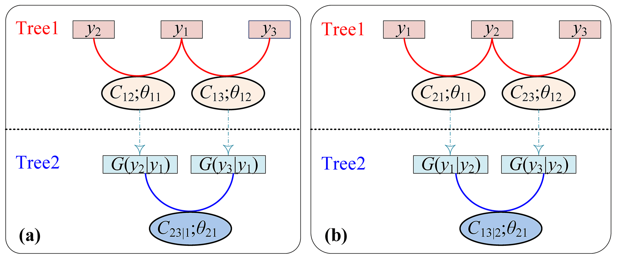
Figure 2 Different schematics (two types) for C-vine copulas using three-dimensional scenarios. For the first type (a), the ordering variables are y₁, y₂, and y₃; for the second type (b), they are y₂, y₁, and y₃. C₁₂(C₂₁), C₁₃(C₂₃), and $C_{\mathrm{23}|\mathrm{1}}\left(C_{\mathrm{13}|\mathrm{2}}\right)$ denote bivariate copulas with parameters of θ₁₁, θ₁₂, and θ₂₁, respectively. Here, θ_ij signifies the parameters of the jth edge with respect to the ith tree. G($\cdot |\cdot$) represents conditional distribution functions.

A conditional copula density needs to be addressed in Eq. (4), i.e., G(y|w), where w is a d-dimensional vector w= (w₁, …, w_d). Here, regarding the conditional distribution of y given the conditions w, we introduced the h function, h(y, w; θ), to indicate G(y| w) as follows (Aas et al., 2009; Joe, 1996):

$$\begin{array}{}\text{(5)}& \begin{array}{rl}h& (y,\mathit{w};\mathit{\theta }):=G\left(y\right|\mathit{w})\\ & ={\displaystyle \frac{\partial C_{y,w_j|{\mathit{w}}_{-j}}\left[G\left(y\right|{\mathit{w}}_{-j}),G(w_j\left|{\mathit{w}}_{-j}\right)\right]}{\partial G\left(w_j\right|{\mathit{w}}_{-j})}},\end{array}\end{array}$$

where θ denotes the parameter(s) of the bivariate-copula function $C_{y{w}_j|{\mathit{w}}_{-j}}$, w_j represents an arbitrary component of w, and w_−j indicates the excluding element w_j from the vector w.

If we set the ordering variables as y₁, y₂, and y₃, the conditional variables as y₁ and y₂, and the predictand as y₃, G(y₃|y₁, y₂), based on Eq. (5), can be expressed as follows:

$$\begin{array}{}\text{(6)}& \begin{array}{rl}G\left(y_{\mathrm{3}}\right|y_{\mathrm{1}},y_{\mathrm{2}})& ={\displaystyle \frac{\partial C_{y_{\mathrm{3}},y_{\mathrm{1}}\left|y_{\mathrm{2}}\right.}\left[G\left(y_{\mathrm{3}}\right|y_{\mathrm{1}}),G(y_{\mathrm{2}}\left|y_{\mathrm{1}}\right)\right]}{\partial G\left(y_{\mathrm{2}}\right|y_{\mathrm{1}})}}\\ & =h\left\{h\left(u_{\mathrm{3}}\left|u_{\mathrm{1}};{\mathit{\theta }}_{\mathrm{12}}\right.\right)\left|h(u_{\mathrm{2}}\left|u_{\mathrm{1}};{\mathit{\theta }}_{\mathrm{11}});{\mathit{\theta }}_{\mathrm{21}}\right.\right.\right\}.\end{array}\end{array}$$

Here, θ_ij (where i denotes a tree and j is an edge) represents the parameters of different conditional copulas in the 3C-vine model (Fig. 2a), and u_k (k= 1, 2, 3) is the marginal CDF of y_k. The CDF for each variable is substituted by the corresponding empirical Gringorten cumulative probability (Bevacqua et al., 2017b; Genest et al., 2009; Wu et al., 2021b).

Next, we introduced the τth copula–quantile curve (Chen et al., 2009; Liu et al., 2018) to simulate u₃ based on Eq. (6) and derived its inverse distribution function as follows:

$$\begin{array}{}\text{(7)}& \begin{array}{rl}{y}_{\mathrm{3}}& =N^{-\mathrm{1}}\left\{G\left(\mathit{\tau }\right|y_{\mathrm{1}},y_{\mathrm{2}})\right\}=N^{-\mathrm{1}}\left(u_{\mathrm{3}}\right)\\ & =N^{-\mathrm{1}}\left[h^{-\mathrm{1}}\left\{h^{-\mathrm{1}}(\mathit{\tau }\left|h(u_{\mathrm{2}}\left|u_{\mathrm{1}};{\mathit{\theta }}_{\mathrm{11}});{\mathit{\theta }}_{\mathrm{21}})\left|u_{\mathrm{1}};{\mathit{\theta }}_{\mathrm{12}}\right.\right.\right.\right\}\right],\end{array}\end{array}$$

where N⁻¹ and h⁻¹ signify the inverse forms of the Gaussian distribution and the h function, respectively; y₃ is the forecasted agricultural drought at time t (i.e., SSI_t); and y₁ and y₂ are the predictors corresponding to the antecedent meteorological drought and agricultural drought persistence at time t−i (i.e., SPI_t−i and SSI_t−i, respectively). The “BiCopHfunc” and “BiCopHinv” R functions in the “VineCopula” R package (Nagler et al., 2021) were utilized to model the h function and its inverse form for Eq. (7), respectively.

The tree structure is related to the ordering variables; thus, when the ordering variables are y₂, y₁, and y₃ (conditional variables are y₁ and y₂; Fig. 2b), Eqs. (6) and (7) can be changed analogously as follows:

$$\begin{array}{}\text{(8)}& {\displaystyle }G\left(y_{\mathrm{3}}\left|y_{\mathrm{2}},y_{\mathrm{1}}\right.\right)=h\left\{h\left(u_{\mathrm{3}}\left|u_{\mathrm{2}};{\mathit{\theta }}_{\mathrm{12}}\right.\right)\left|h(u_{\mathrm{1}}\left|u_{\mathrm{2}};{\mathit{\theta }}_{\mathrm{11}});{\mathit{\theta }}_{\mathrm{21}}\right.\right.\right\};\text{(9)}& {\displaystyle }\begin{array}{rl}{y}_{\mathrm{3}}& =N^{-\mathrm{1}}\left(u_{\mathrm{3}}\right)=N^{-\mathrm{1}}\\ & \left[h^{-\mathrm{1}}\left\{h^{-\mathrm{1}}(\mathit{\tau }\left|h(u_{\mathrm{1}}\left|u_{\mathrm{2}};{\mathit{\theta }}_{\mathrm{11}});{\mathit{\theta }}_{\mathrm{21}})\left|u_{\mathrm{2}};{\mathit{\theta }}_{\mathrm{12}}\right.\right.\right.\right\}\right].\end{array}\end{array}$$

For agricultural drought forecast via the 3C-vine model (see Fig. 3 for details), we first selected the best 3C-vine model (i.e., selected the best model from Eqs. (7) and (9) according to the minimum AIC). A sample size of 1,000 uniformly distributed random values was then generated over the [0, 1] interval using Monte Carlo simulation. Finally, the best 3C-vine model was utilized to obtain 1000 simulations (or estimations) of $y_{\mathrm{3}}^{\mathrm{yr}}$. The best forecast of $y_{\mathrm{3}}^{\mathrm{yr}}$ was finally calculated using the mean value of these simulations. Note that leave-one-out cross-validation (LOOCV) (Wilks, 2020) is applied to forecast agricultural drought for each grid cell in August of every year during 1961–2018 based on the 3C-vine model or MG model, namely, each time one sample (or observation) was left for validation, and the rest were used to establish the 3C-vine model or MG model and obtain the corresponding parameters of these models. In other words, this process was repeated 58 times (the length of years used in this study) for a specific grid cell.

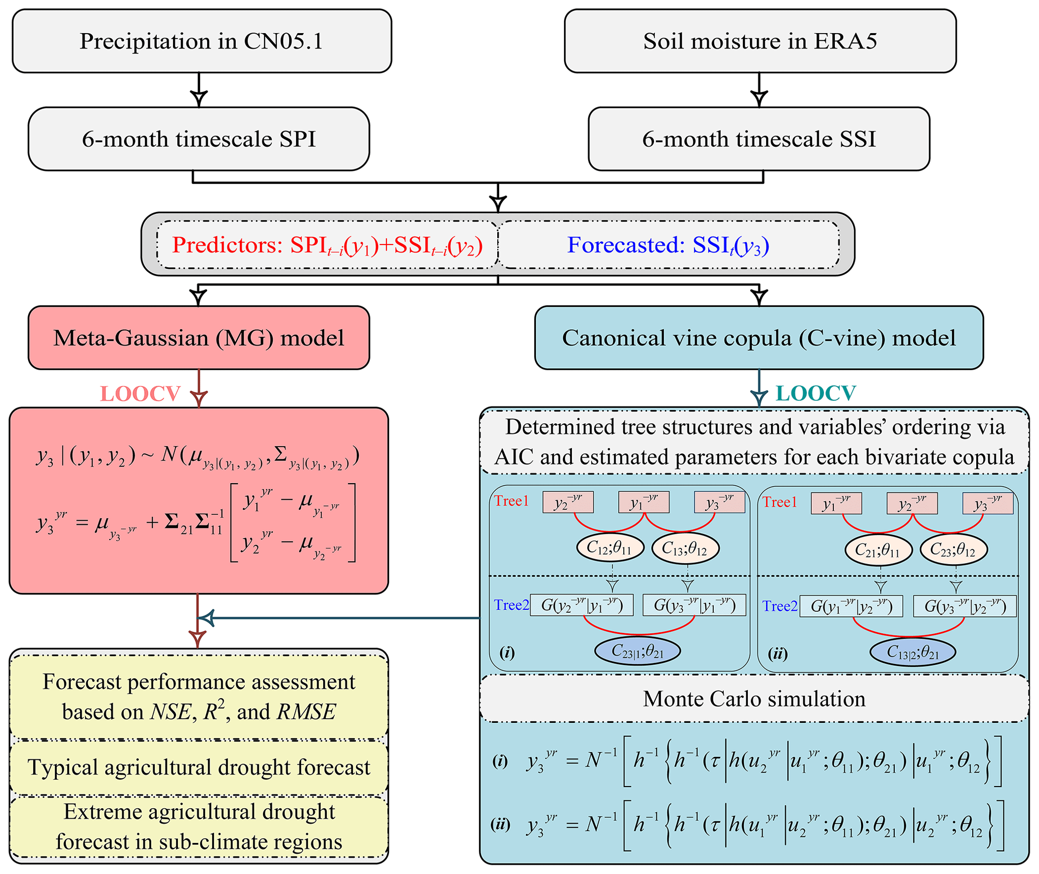
Figure 3 Flowchart of agricultural drought forecasting based on the canonical vine copulas (3C-vine) and meta-Gaussian (MG) models using three-dimensional scenarios. Here, t denotes the target month (e.g., August), i signifies the lead times (1–3 months), LOOCV stands for leave-one-out cross-validation, $y_{\mathrm{1}}^{-\mathrm{yr}}\left(y_{\mathrm{2}}^{-\mathrm{yr}}\right)$ indicates the series after removing a sample ($y_{\mathrm{1}}^{\mathrm{yr}}\left(y_{\mathrm{2}}^{\mathrm{yr}}\right))$ for a specific year, and $y_{\mathrm{3}}^{\mathrm{yr}}$ is the agricultural drought forecast value for the target month of a specific year. Note that the optimal tree structure (i or ii on the right-hand side of this figure) is selected based on the AIC to forecast agricultural drought.

3.3 Performance metrics

Three evaluation metrics – the Nash–Sutcliffe efficiency (NSE), the coefficient of determination (R²), and the root-mean-square error (RMSE) – were utilized to assess the forecast performance of the 3C-vine and MG models. These metrics can be expressed as follows:

$$\begin{array}{}\text{(10)}& {\displaystyle }\mathrm{NSE}=\mathrm{1}-{\displaystyle \frac{\sum _{i=\mathrm{1}}^n({\mathrm{AP}}_i-{\mathrm{AO}}_i{)}^{\mathrm{2}}}{\sum _{i=\mathrm{1}}^n({\mathrm{AO}}_i-\stackrel{\mathrm{‾}}{\mathrm{AO}}{)}^{\mathrm{2}}}}\mathrm{NSE}\in (-\mathrm{\infty },\mathrm{1}];\text{(11)}& {\displaystyle }{R}^{\mathrm{2}}={\displaystyle \frac{{\left[\sum _{i=\mathrm{1}}^n({\mathrm{AO}}_i-\stackrel{\mathrm{‾}}{\mathrm{AO}})({\mathrm{AP}}_i-\stackrel{\mathrm{‾}}{\mathrm{AP}})\right]}^{\mathrm{2}}}{\sum _{i=\mathrm{1}}^n({\mathrm{AO}}_i-\stackrel{\mathrm{‾}}{\mathrm{AO}}{)}^{\mathrm{2}}\cdot \sum _{i=\mathrm{1}}^n({\mathrm{AP}}_i-\stackrel{\mathrm{‾}}{\mathrm{AP}}{)}^{\mathrm{2}}}}{R}^{\mathrm{2}}\in [\mathrm{0},\mathrm{1}];\text{(12)}& {\displaystyle }\mathrm{RMSE}=\sqrt{{\displaystyle \frac{\mathrm{1}}{n}}\sum _{i=\mathrm{1}}^n({\mathrm{AP}}_i-{\mathrm{AO}}_i{)}^{\mathrm{2}}}\mathrm{RMSE}\in [\mathrm{0},+\mathrm{\infty }).\end{array}$$

Here, n is the number of forecast periods; AO_i and AP_i are the ith observed and forecasted agricultural droughts (i.e., SSI), respectively; and $\stackrel{\mathrm{‾}}{\mathrm{AO}}$ and $\stackrel{\mathrm{‾}}{\mathrm{AP}}$ denote the mean of the SSI observations and forecasts in the target month (e.g., August), respectively. Moreover, a more positive NSE and R² value and a lower RMSE value indicate good forecast performance for the 3C-vine or MG models.

4 Results

4.1 Correlation patterns of agricultural drought with potential predictors

The dependence between variables can be measured by the correlation coefficient, which indirectly characterizes the quantity of common information between two variables. We employed Kendall's correlation coefficient (τ_k) to measure the dependence of agricultural drought at current time t (SSI_t, where t is August in this work) on the previous meteorological drought (SPI_t−i, where i indicates the 1- to 3-month lag or lead times in this work) and agricultural drought persistence (SSI_t−i). It should be mentioned that the widely used significant correlation threshold may overestimate or overinterpret the dependence between variables (Wilks, 2016). Therefore, we adopted the maximum false discovery rate (FDR) of 0.1 to correct τ_k at the 0.05 significance level (Benjamini and Hochberg, 1995; Röthlisberger and Martius, 2019; Wilks, 2016).

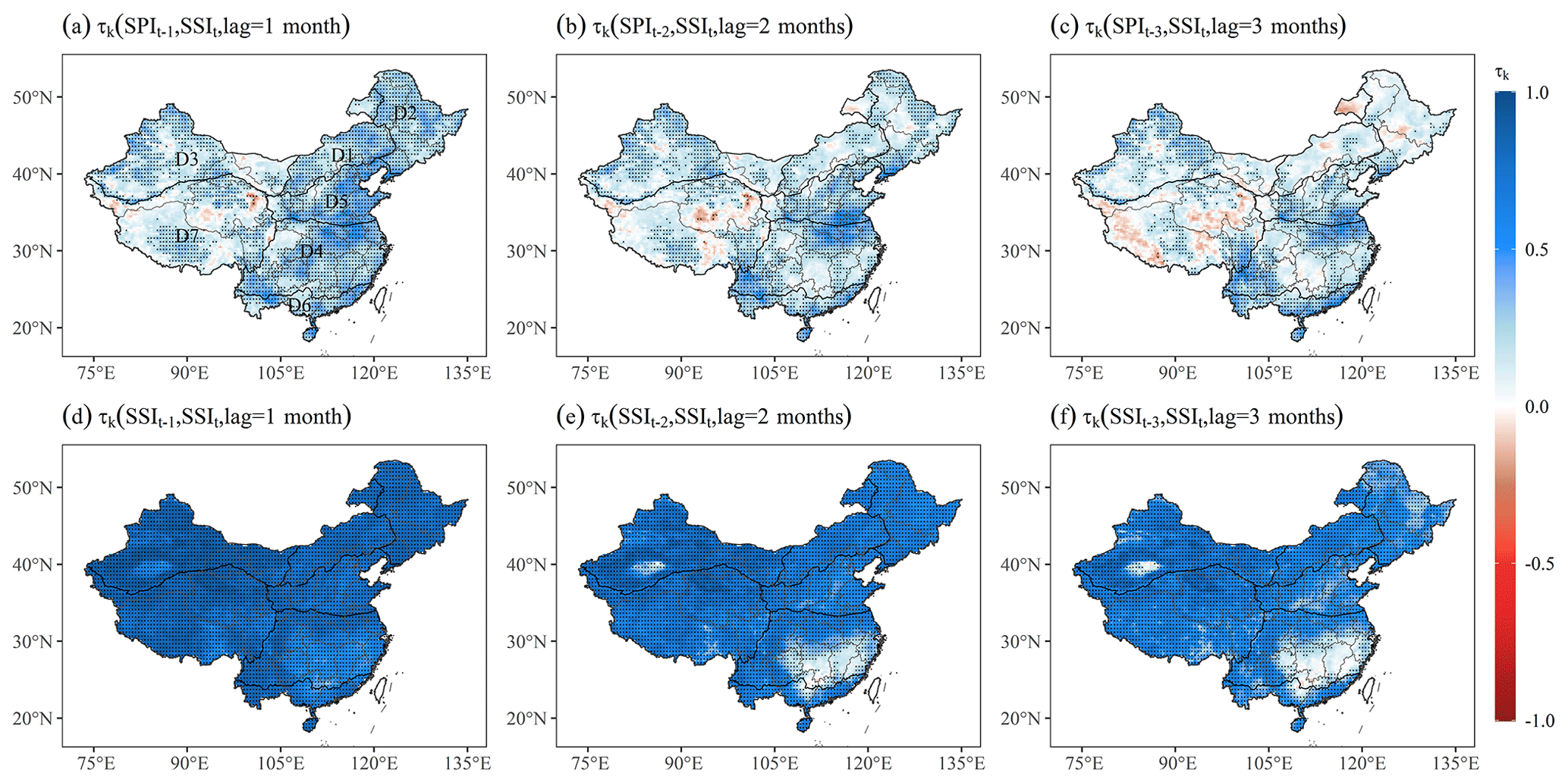
Figure 4 Spatial patterns of 1- to 3-month lag times for the Kendall's correlation coefficient (τ_k) between SPI_t−i and SSI_t (where t denotes August, and i is the 1- to 3-month lag time) (top row) and between SSI_t−i and SSI_t (bottom row) for August during 1961–2018 over China. Note that the stippling indicates where τ_k is at a 0.05 significance level, which is corrected via the false discovery rate (FDR) of 0.1.

Figure 4 summarizes the 1- to 3-month lag τ_k between an antecedent SPI (SSI) and succedent SSI for August during 1961–2018 over China. For most regions of China, the previous meteorological drought or agricultural drought persistence (memory) showed significant positive correlations (i.e., stippling in Fig. 4) with the target agricultural drought when using 1- to 3-month lag times. Moreover, we found perfect agricultural drought memory over many regions of China (excluding D4, a humid climate region; Fig. 4e, f), as overlapping information existed in SSI_t and SSI_t−i. Additionally, the dependency pattern varied both temporally and spatially, and this phenomenon evidently occurred with the lag (or lead) time extended, especially between SPI_t−i and SSI_t (Fig. 4a, b, c). Overall, the prior meteorological drought and agricultural drought memory provided reliable and useful forecast information for subsequent agricultural drought for most areas of China.

4.2 Forecast performance comparison between the 3C-vine and MG models

We leveraged the MG model as a reference model to measure the performance of the 3C-vine model with respect to forecasting agricultural drought for the 1961–2018 period over China. Figure 5a–i show the difference in the NSE, R², and RMSE between the 3C-vine and MG models (i.e., ΔNSE = NSE_3C − NSE_MG; $\mathrm{\Delta }{R}^{\mathrm{2}}=R_{\mathrm{3}\mathrm{C}}^{\mathrm{2}}$ − $R_{\mathrm{MG}}^{\mathrm{2}}$; and ΔRMSE = RMSE_3C −RMSE_MG) for respective 1- to 3-month lead times for August. In terms of the spatial extent of ΔNSE > 0, ΔR² > 0, and ΔRMSE < 0, the agricultural drought forecast ability of the 3C-vine model was superior to the MG model, which occupied 65 %, 68 %, and 58 % of land areas in China, respectively, for the 1-month lead SSI forecast (Fig. 5a, d, g). The relationship between the predictors and the forecasted variable was simple at a 1-month lead time; thus, the MG model better showed their connection. However, when using a prolonged lead time, the forecast skill of the 3C-vine model was superior to the MG model for most regions of China, accounting for 72 % and 74 % of land areas in China for ΔR² > 0 for 2- and 3-month lead times, respectively (e.g., Fig. 5e, f). This indicates the 3C-vine model sufficiently utilized the forecasted information on previous meteorological drought and agricultural drought persistence, in contrast with the MG model under the same conditions.

Figure 5 Forecast performance based on (a)–(c) ΔNSE (the difference in NSE between the 3C-vine and MG models, NSE_3C − NSE_MG), (d–f) ΔR² ($R_{\mathrm{3}\mathrm{C}}^{\mathrm{2}}$ − $R_{\mathrm{MG}}^{\mathrm{2}}$), and (g–i) ΔRMSE (RMSE_3C − RMSE_MG) for the 1- to 3-month lead times in August during 1961–2018 over China. The corresponding box plots of (j) ΔNSE, (k) ΔR², and (l) ΔRMSE relative to a threshold of zero (horizontal black dash line) for agricultural drought forecast in August for 1- and 3-month lead times in climate regions D1–D7 over China are also shown. The percentages of ΔNSE > 0, ΔR² > 0, and ΔRMSE < 0 are listed in the bottom left of the corresponding subfigures.

The forecast ability of the 3C-vine model, compared with the MG model, is limited over climate region D5 (e.g., Fig. 5b, c). This may be related to the fact that D5 is a crucial grain-producing region in China (Lu et al., 2012; Xiao et al., 2019; Zhang et al., 2016), and the related intensive anthropogenic activities (e.g., irrigation and urbanization) in the area may alter the linkage between meteorological drought and agricultural drought as well as the strength of the agricultural drought memory (AghaKouchak et al., 2021). To ensure food security, if D5 had experienced a drought event at the previous stage, agricultural managers and policymakers would have mitigated the drought through irrigation in a variety of ways, such as groundwater exploitation and reservoir operation (Zhang et al., 2016). However, in this case, the soil water obtaining the supplement from the irrigation water would affect the performance of agricultural drought forecast. Thus, in contrast with the MG model, the 3C-vine model yielded a better forecast performance for August under 1- to 3-month lead times for agricultural drought across most areas of China, except for the climate region D5.

4.3 Case study and subclimate region assessment

A severe drought hit most regions of China in summer 2018, especially southern and northern China, due to the abnormal impact of the western North Pacific subtropical high (Liu and Zhu, 2019; Zhang et al., 2020; Y. Zhang et al., 2018). We chose the agricultural drought that occurred in August of 2018 as a case study to investigate the forecast ability of the 3C-vine model. The MG model was selected as a benchmark model. Figure 6 presents the SSI observations and the 1- to 3-month lead time SSI forecasts for this agricultural drought using the 3C-vine and MG models. Obviously, the 1- to 3-month lead time SSI forecasts from the 3C-vine model resembled the observations (Fig. 6a, b, c, d), which captured the droughts that emerged in southern China, northern China, and northeastern China (i.e., climate regions D1–D2 and D4–D6). Comparing the 3C-vine model with the MG model using 2- to 3-month lead times (Fig. 6a, b, c, and d versus Fig. 6f and g), we observed the deteriorating forecast skill of the MG model in climate region D5, which tended toward a non-drought state (i.e., SSI > 0), but the 3C-vine model better forecasted the agricultural drought for these regions under the same conditions, although the severity of agricultural drought had some decrement. The above analyses indicated that the 3C-vine model, using previous meteorological drought and agricultural drought persistence as two predictors, had the ability to reliably forecast drought over many regions of China.

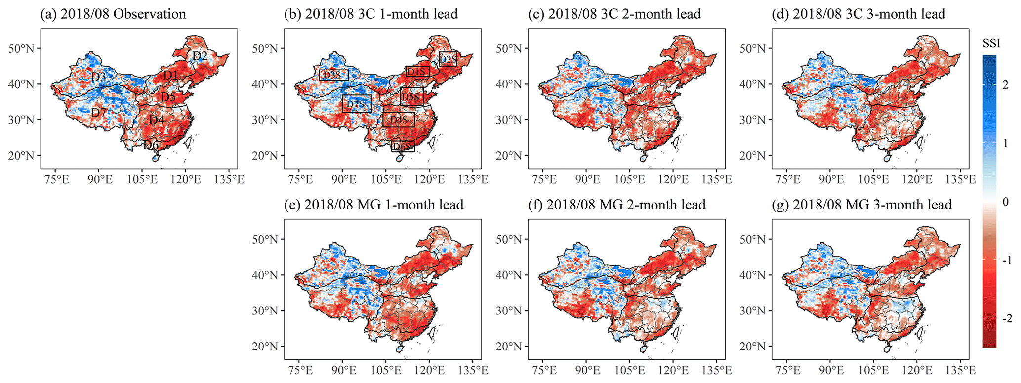
Figure 6 SSI observations in August of 2018 (a) as well as the corresponding SSI forecasts for 1- to 3-month lead times utilizing the 3C-vine model (b–d) and the MG model (e–g) over China. The black rectangles (as shown in b) denote the typical areas (corresponding to D1S–D7S) selected in climate regions D1–D7.

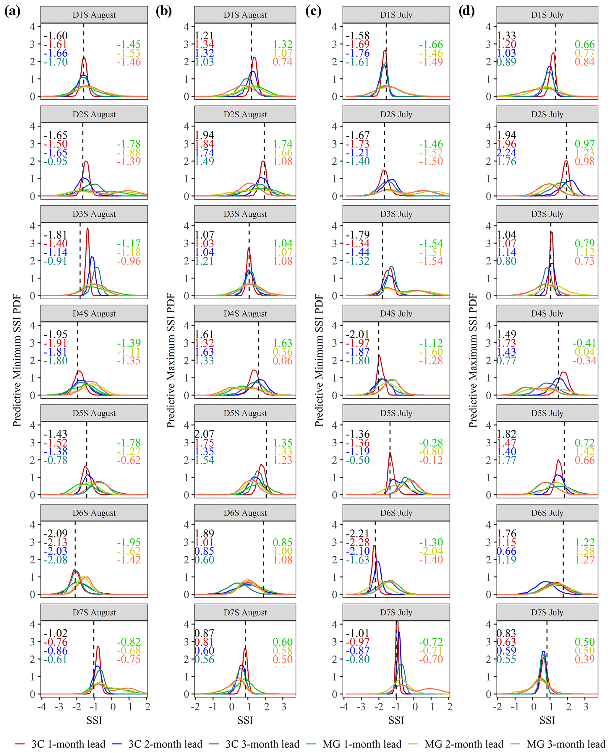
Figure 7 Probability density function (PDF) curve of minimum (a, c) and maximum (b, d) SSI for 1- to 3-month lead times for August (a, b) and July (c, d) during the 1961–2018 period over seven selected typical areas in the climate regions D1–D7 (i.e., the black rectangles in Fig. 6b signify regions D1S–D7S; see labels). The black dashed line and text indicate the minimum and maximum SSI observations in August and July over D1S–D7S. The red (green), blue (yellow), and cyan (coral) text on the left (right) of each subfigure denote SSI forecasts for 1- to 3-month lead times in August or July from the 3C-vine model (MG model), which correspond to the abscissa projected by the peak point of each PDF.

Furthermore, to explore the skill of the 3C-vine model with respect to capturing the extrema of agricultural drought (i.e., minimum and maximum SSIs), we randomly selected a typical area (black rectangles in Fig. 6b) in each climate region. Note that these extreme SSI values were calculated using the spatial average in each typical region. Figure 7a and b show the probability density function (PDF) curves of the minimum and maximum SSIs for these selected typical regions (D1S–D7S) using the 3C-vine and MG models for 1- to 3-month lead times in August. Here, the vertical black dashed line denotes the SSI observation in each subplot. The x-axis value of the peak point (i.e., high probability) for each PDF curve is regarded as the best estimation of the SSI for diverse lead times. Using the 3C-vine model as an example (as for the MG model), for a minimum SSI with 1- to 2-month lead times, the differences between the forecasted SSI and the observed SSI were slight (except for D3S), and all cases reflected the drought state for these typical regions (Fig. 7a). The deteriorated skill of the 3C-vine and MG models in region D3S may be attributed to the lengthy response time existing between precipitation deficiency and soil moisture shortage, which is caused by limited precipitation that cannot effectively replenish soil moisture depletion due to the incrassation of the vadose zone. For the 3-month lead time, poor forecasts were produced in region D5S for the minimum SSI. This phenomenon may result in the agricultural manager utilizing irrigation to mitigate the effect of drought on crop growth; thus, the response relationship between meteorological drought and agricultural drought accordingly would change (Y. Xu et al., 2021).

For the maximum SSI forecasted utilizing the 3C-vine model (as for the MG model) over diverse regions, excellence forecast ability is displayed for the 1- to 3-month lead times (Fig. 7b), excluding regions D5S and D6S (PDF curve shifted left). Due to abundant precipitation and a higher soil moisture content in D6S, the shortened response time between precipitation and soil moisture (Y. Xu et al., 2021) may cause inferior forecasts for the 3C-vine model for the target month.

To display the robustness of the 3C-vine model with respect to forecasting agricultural drought in any month of interest, we further forecasted extreme agricultural drought in July for D1S–D7S (Fig. 7c, d). The difference between the forecasted and observed extreme SSIs for the MG model is larger than that for the 3C-vine model in distinct typical regions, e.g., the forecasted maximum SSI in July for D4S (Fig. 7d). The width of the PDF curve qualitatively provides an estimation of the forecast uncertainty of the 3C-vine and MG models. As shown in Fig. 7, in comparison with the 3C-vine model, we found that the width of the PDF curves of the MG model are broadened, indicating that the MG model produced more pronounced uncertainty with respect to agricultural drought forecast. Furthermore, the skill of the MG model tended to deteriorate over many selected typical regions, especially for 2- to 3-month lead times in July and August. Generally, compared with the MG model using different lead times, agricultural drought forecasts made by the 3C-vine model are more accurate across different typical regions, in terms of predictive uncertainty (i.e., the width of PDF curve) as well as the difference between observed and forecasted extreme SSIs (Fig. 7).

Moreover, to assess the forecast performance (according to the NSE, R², and RMSE) of the 3C-vine model over each climate region, we counted the pixels contained in each climate region and constructed box plots for these performance metrics (Fig. 5j, k, l). We still selected the MG model as the reference model and obtained the difference between these two models (i.e., ΔNSE, ΔR², and ΔRMSE). The forecast performance of the 3C-vine and MG models was generally consistent for a 1-month lead time for August over climate regions D1–D7 (the median percentiles of ΔNSE, ΔR², and ΔRMSE were all around the zero line; Fig. 5j, k, l), indicating that the improved skill of the 3C-vine model was limited under the same conditions. Obviously, the median percentiles of ΔNSE and ΔR² were greater than zero and ΔRMSE was lower than zero for the 2- to 3-month lead time SSI forecasts for August in the different climate regions D1–D7 (except for D5), indicating that the 3C-vine model shows better performance than the MG model with respect to forecasting agricultural drought over diverse climate regions of China.

In conclusion, based the ability of typical agricultural drought forecasts (Fig. 6), the agricultural drought extrema captured in selected typical regions (Fig. 7), and the comprehensive forecast performance shown in diverse climate regions (Fig. 5j, k, l), the 3C-vine model had a good forecast skill for 1- to 3-month lead times for agricultural drought in August over most areas of China.

5 Discussion and conclusions

This study developed a C-vine copula model to forecast agricultural drought over China in three dimensions in which antecedent meteorological drought and agricultural drought persistence were employed as two predictors. We selected the MG model as a reference, in terms of the difference in NSE, R², and RMSE between the 3C-vine and MG models, in order to evaluate the forecast performance of the 3C-vine model. These performance metrics all showed that the 3C-vine model, especially for 2- to 3-month lead times, outperformed the MG model in many climate regions over China (except for D5, which lies in the humid and subhumid regions of northern China) (Fig. 5). Compared with the MG model, the 3C-vine model yielded good forecast skill for the selected typical agricultural droughts (Fig. 5). Furthermore, the nearly perfect forecast of extrema agricultural drought in typical regions (Fig. 7) further certified the excellent ability of the 3C-vine model.

Heterogeneous topography and anthropogenic activities (e.g., irrigation and urbanization) have certainly impacted precipitation interpolation and soil moisture simulation, which may depart from the actual precipitation or soil moisture conditions; notwithstanding, the precipitation of CN05.1 and the soil moisture of ERA5 show good performance with respect to drought monitoring and forecasting over China (Wang and Yuan, 2021; Wu et al., 2021b; Xu et al., 2009; T. Zhang et al., 2021; X. Zhang et al., 2019). The abovementioned factors can also influence the response (propagation) time from meteorological drought to agricultural drought as well as agricultural drought memory and can, thus, lead to the 3C-vine model falling short in some climate regions. To address this issue, we can comprehensively utilize multiple reanalysis data sets, e.g., the precipitation and soil moisture data in Global Land Data Assimilation System (GLDAS) and ERA5, to reduce the uncertainty resulting from a single data source (Wang and Yuan, 2021; Wu et al., 2021b). Currently, it is a challenge to consider irrigation activities in agricultural drought forecasting, especially at large spatial scales. In addition to the antecedent precipitation deficit, air temperature, relative humidity, and evapotranspiration may influence the soil moisture budget. Moreover, from the perspective of driving mechanisms, the effects of certain atmospheric circulation anomalies (e.g., the El Niño–Southern Oscillation, ENSO; the Pacific Decadal Oscillation, PDO; the and North Arctic Oscillation, NAO) on agricultural drought at regional and global scales can also be considered as predictors (Y. Zhang et al., 2021). Therefore, a more efficient space can be established by leveraging these predictors for forecasting agricultural drought.

In recent years, a myriad of extreme events, such as heat waves and flash droughts, have swept many regions around the globe (Wu et al., 2021a). These extreme events have a rapid onset of a few days or weeks and lead to devastating impacts on agricultural production, water resource security, and human well-being (Wang and Yuan, 2021; Yuan et al., 2019; Zscheischler et al., 2020). Therefore, agricultural drought forecasting at finer temporal scales (e.g., weekly) is essential for agricultural managers and policymakers to manage and plan water use. However, with the limited spatiotemporal resolution and the length of model samples, agricultural drought forecasting has not been carried out at sub-monthly or pentad temporal scales.

The limitation of this study is that we choose a “best” model from two C-vine copula candidate models (i.e., Fig. 2) as the ideal forecast. However, due to the inherent structural differences (i.e., ordering variables are different), the utilized best model may underestimate the forecast uncertainty (Liu et al., 2021a). Therefore, to reduce the predictive uncertainty and improve the forecast performance, a multi-model combination technique (e.g., Bayesian model averaging; Liu et al., 2021a; Long et al., 2017) could be considered to merge different C-vine copula candidate models. Moreover, as we only focused on C-vine copulas and several bivariate-copula functions, other D-vine copulas or regular vine copulas as well as a multitude of bivariate-copula families (Sadegh et al., 2017) could be investigated to establish the forecast model for agricultural drought in following work.