the Creative Commons Attribution 4.0 License.
the Creative Commons Attribution 4.0 License.
 | 20 Jun 2022
Seasonal forecasting of lake water quality and algal bloom risk using a continuous Gaussian Bayesian network
Leah A. Jackson-Blake
François Clayer
Sigrid Haande
James E. Sample
S. Jannicke Moe
Freshwater management is challenging, and advance warning that poor water quality was likely, a season ahead, could allow for preventative measures to be put in place. To this end, we developed a Bayesian network (BN) for seasonal lake water quality prediction. BNs have become popular in recent years, but the vast majority are discrete. Here, we developed a Gaussian Bayesian network (GBN), a simple class of continuous BN. The aim was to forecast, in spring, mean total phosphorus (TP) and chlorophyll a (chl a) concentration, mean water colour, and maximum cyanobacteria biovolume for the upcoming growing season (May–October) in Vansjø, a shallow nutrient-rich lake in southeastern Norway. To develop the model, we first identified controls on interannual variability in seasonally aggregated water quality. These variables were then included in a GBN, and conditional probability densities were fit using observations (≤39 years). GBN predictions had R2 values of 0.37 (chl a) to 0.75 (colour) and classification errors of 32 % (TP) to 17 % (cyanobacteria). For all but lake colour, including weather variables did not improve the predictive performance (assessed through cross-validation). Overall, we found the GBN approach to be well suited to seasonal water quality forecasting. It was straightforward to produce probabilistic predictions, including the probability of exceeding management-relevant thresholds. The GBN could be sensibly parameterised using only the observed data, despite the small dataset. Developing a comparable discrete BN was much more subjective and time-consuming. Although low interannual variability and high temporal autocorrelation in the study lake meant the GBN performed only slightly better than a seasonal naïve forecast (where the forecasted value is simply the value observed the previous growing season), we believe that the forecasting approach presented here could be particularly useful in areas with higher sensitivity to catchment nutrient delivery and seasonal climate and for forecasting at shorter (daily or monthly) timescales. Despite the parametric constraints of GBNs, their simplicity, together with the relative accessibility of BN software with GBN handling, means they are a good first choice for BN development with continuous variables.
- Article
(5262 KB) - Full-text XML
- BibTeX
- EndNote


Despite their importance, freshwaters are under intense pressure from human activities. Severe declines in the quantity and quality of habitats and species abundance are widespread, and freshwaters are now one of the most threatened ecosystem types in large parts of the world (Gozlan et al., 2019; Reid et al., 2019; Dudgeon et al., 2006). To try to safeguard freshwater condition, the EU Water Framework Directive (WFD) requires all waterbodies to achieve at least “good” ecological status by 2027, assessed using a set of indicators of ecosystem integrity (ECOSTAT, 2005). However, meeting WFD targets is challenging, and despite widespread implementation of measures to improve water quality, 60 % of European surface waters were still below good ecological status in 2018 (Kristensen et al., 2018). Harmful cyanobacterial blooms are a particular concern worldwide, as they can produce harmful toxins, damage ecosystems, and jeopardise drinking water supplies, fisheries and recreational areas. Harmful blooms are becoming more widespread, frequent, and intense due to eutrophication and climate change (Ibelings et al., 2016; Huisman et al., 2018; Taranu et al., 2015).
Advance warning, a season in advance, that poor water quality was likely could allow for measures to be put in place to reduce the impacts. For example, water levels could be raised or lowered in flow-regulated waterbodies or more stringent farm management or effluent discharge advice could be issued. Although many cyanobacteria forecasting systems have been developed, the majority predict conditions at most a month in advance or focus on multidecadal predictions (reviewed in Rousso et al., 2020). Seasonal forecasts, issued with lead times of 1–6 months, could allow for more comprehensive preventative or mitigative measures. Seasonal forecasting is a growing area of research, taking advantage of developments in seasonal climate forecasting, and there are many potential management applications (Bruno Soares and Dessai, 2016). However, seasonal forecasting within the water sector has so far been largely focused on streamflow forecasting, with very limited applications to lake water quality forecasting. The focus of the WATExR project, a European Union project funded by the European Research Area for Climate Services (ERA4CS), was to help address this gap by developing pilot seasonal forecasting tools for lake water quality and ecology. Tools were co-developed with water managers at five catchment–lake case study sites, with four in Europe and one in South Australia (Jackson-Blake et al., 2022). Tools linked seasonal climate forecasts with models for predicting river discharge, lake water level and water temperature (Mercado-Bettín et al., 2021), water quality, algal bloom risk, and fish migration. Here, we describe the model developed to forecast lake water quality at one of the case study sites, Vansjø in Norway.
A multitude of potential methods exists for water quality modelling and forecasting. Here, we adopt a Bayesian network (BN) approach. BNs are a type of probabilistic multivariate model which is well suited to environmental modelling, risk assessment, and forecasting (Aguilera et al., 2011; Kaikkonen et al., 2021; Uusitalo, 2007). In brief, BNs are graphical models in which the joint probability distribution among a set of variables X=[X1, … Xn] is represented in terms of (1) a directed acyclic graph, where each vertex (or node) represents a variable in the model and an edge (or arc) linking two variables indicates statistical dependence, and (2) conditional distributions for each variable Xi, p(Xi|pa(Xi)), given the probability distribution pa(Xi) of any parent nodes, which quantify the strength and shape of dependencies between variables (Pearl, 1986). In recent years, BNs have become popular in a broad range of environmental modelling disciplines, including modelling lake water quality and algal bloom risk (e.g. Shan et al., 2019; Rigosi et al., 2015; Williams and Cole, 2013; Couture et al., 2018; Gudimov et al., 2012). Particular strengths in terms of our seasonal forecasting aims are that, as nodes are modelled using probability distributions, risk and uncertainty can be estimated easily and accurately compared to many other modelling approaches. They can thus be powerful tools to assess the probability of events (e.g. WFD ecological status class). They are also well suited for communicating and visualising the model to end-users, and it is easy to update the model given new data. Other benefits include the ability to model complex systems in a quick and efficient way, to combine data and expert knowledge, easy handling of missing values, and the potential to be used for inference, as well as prediction.
BNs were originally designed to deal with discrete data. Relationships between nodes in discrete BNs can be nonlinear and complex, thereby allowing for the full power of BN analysis, and the vast majority of environmental BN models are discrete (Aguilera et al., 2011). When using a discrete BN, any continuous variables must first be discretised. However, this involves an information loss as discretisation can only capture the rough characteristics of the original distribution. In addition, discretisation choices (number of intervals and division points) affect BN results (e.g. Nojavan et al., 2017) and their interpretation (Qian and Miltner, 2015). In practice, it is usually necessary to restrict the number of intervals, often to just two or three classes, as the more intervals there are, the more data are needed to parameterise the model meaningfully (Hanea et al., 2015). Such restrictions mean that it then becomes difficult to capture complex relationships, thereby diminishing the theoretical benefits of using a discrete network (Uusitalo, 2007). Continuous BNs, by contrast, represent continuous variables using continuous statistical distributions and therefore avoid the need for discretisation. Hybrid BNs, which include both discrete and continuous nodes, have similar benefits.
In recent years, much focus on continuous networks has been aimed at developing algorithms for nonparametric networks, i.e. continuous networks which are not limited by assumptions about the nature of the statistical distribution of continuous variables (Marcot and Penman, 2019). However, Gaussian BNs (GBNs) are a long-established, simple, and powerful class of continuous BN and are often the only type of continuous node available in commonly used BN software (e.g. Bayes server, bnlearn, and Hugin). In GBNs, each random variable is defined by a Gaussian distribution, and variables are linearly related to their parents (Geiger and Heckerman, 1994; Shachter and Kenley, 1989). In some situations, these parametric constraints may be overly limiting, but when this approximation is appropriate, GBNs may be preferable over discretisation. Despite the potential benefits, the use of continuous BNs in environmental modelling is rare. In a review of papers published over the period 1990–2010, Aguilera et al. (2011) found only 6 % included continuous or hybrid nodes, and we could only find nine more recent examples in the literature (Web of Science search in November 2021, with the terms [environmental AND modelling* AND “Bayesian network” AND continuous], with a manual sorting of the results).
The overall aims of the paper are, therefore, (1) to develop a model for the seasonal forecasting of lake water quality and (2) to demonstrate the use of a continuous GBN, compared to more traditional discrete BN approaches. Our case study site is the western basin of Vansjø, a shallow mesotrophic/eutrophic lake in southeastern Norway. A number of BN models have previously been applied in the lake (Couture et al., 2014, 2018; Moe et al., 2016, 2019; Barton et al., 2008), but these were all discrete metamodels, i.e. the BN nodes summarised process-based model simulations, statistical relationships, expert opinion, and/or data distributions, and the studies were focused on the longer-term impacts of climate, land use, and land management change. Here, the aim was to provide medium-term forecasts to support lake management by developing a model able to predict, in the spring of a given year, water quality for the coming growing season (May–October), including the probability of lying within WFD ecological status classes for total phosphorus (TP), chl a, and cyanobacteria. We also forecast lake colour, as elevated lake organic matter content (and associated colour) can cause a number of problems for drinking water treatment (e.g. Matilainen et al., 2010).
To develop the model, we take a data-driven approach, where we first use exploratory statistical analyses to identify the main controls on interannual variability in lake water quality and then combine the results of this with domain knowledge to develop a GBN. We also develop a comparable discrete BN, using discretised data. We then explore the sources of predictability and the importance of weather variables by comparing predictive performance of GBNs with different model structures within a cross-validation scheme. We also compare the performance of the Gaussian and discrete BNs and the performance of a simple benchmark model, a seasonal naïve forecast (where the forecasted value is simply the value observed the previous growing season). Finally, we discuss (1) the results in terms of the potential and limitations for seasonal forecasting of lake water quality and (2) the pros and cons of GBNs compared to discrete BNs and compared to multiple linear regression (which shares some features with GBNs).
2.1 Case study site
Vansjø is a large lake in southeastern Norway (59∘24′ N 10∘42′ E, 25 m a.s.l.), with a highly agricultural catchment by Norwegian standards (15 % of the 690 km2 catchment is agriculture) with clay- and P-rich soils. The lake has two main basins, Storefjorden in the east (24 km2) and Vanemfjorden in the west (12 km2; Fig. 1). The largest input is the Hobøl River (catchment area 301 km2) which enters Storefjorden, and then water flows from Storefjorden to Vanemfjorden through a narrow channel, and from Vanemfjorden through the Moss River towards the Oslofjord (Fig. 1). Over the period 1989–2018, catchment mean annual air temperature was 7.2 ∘C and annual precipitation was 992 mm yr−1.
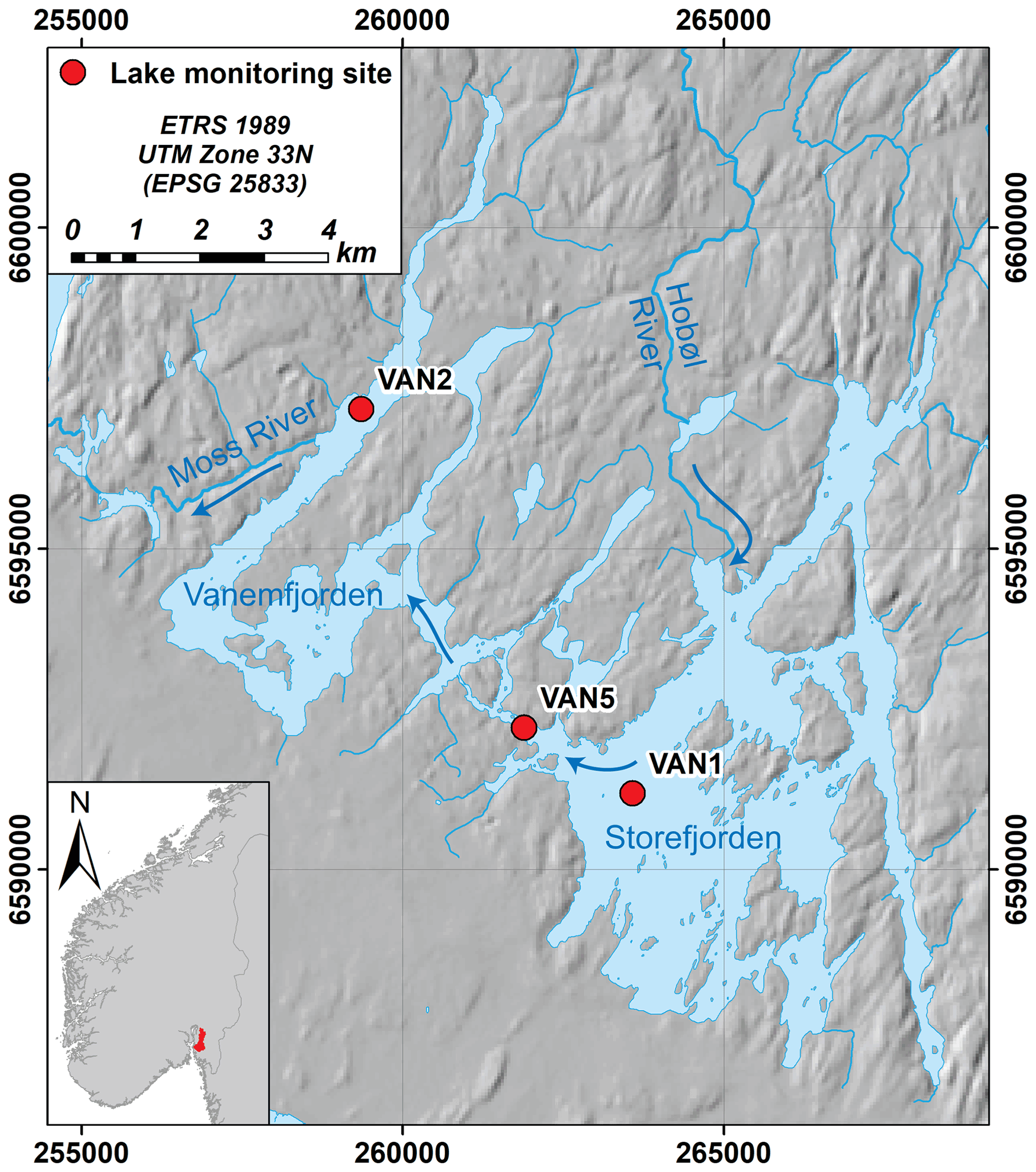
Figure 1Vansjø in southeastern Norway, showing the two main basins, the larger eastern basin (Storefjorden) and Vanemfjorden (the study basin). The two basins are connected by a narrow channel. The largest tributary to Vansjø is the Hobøl River. Main Norwegian Institute for Water Research (NIVA) monitoring sites are shown, and arrows show the dominant flow directions. Here, we use data from VAN2. Hillshade © Kartverket (https://www.kartverket.no/, last access: 9 May 2022); hydrologic data © NVE (https://www.nve.no/english/, last access: 9 May 2022).
Here, we focus on Vanemfjorden, which is shallower (mean depth 3.8 m; max depth 19 m) and more susceptible to eutrophication and cyanobacterial blooms than Storefjorden due to stronger interactions between the water column and the P-rich lake sediments and a more agricultural local catchment. Vanemfjorden has a relatively short residence time (0.21 years), and the water column remains oxygenated throughout the year. Vanemfjorden has a long history of eutrophication and is usually in WFD “moderate” ecological status for mean growing season TP (>20 µg L−1), chl a (>10.5 mg L−1), and maximum cyanobacteria (>1.0 mg L−1; Skarbøvik et al., 2021). Vanemfjorden suffers from toxin-producing cyanobacterial blooms, and bathing bans were in place during much of the early 2000s (Haande et al., 2011).
The outlet of Vanemfjorden is dammed, and the lake water level is regulated for hydropower, recreation, and flood protection. There is a management opportunity for the dam operators to adjust the water level in advance of an anticipated wet, dry, or hot season if problematic water quality is expected. In addition, the local catchment management group (Morsa), responsible for WFD implementation, is interested in seasonal water quality forecasts to inform their management and monitoring plan and, in particular, preparedness for cyanobacterial blooms.
2.2 Overview of the workflow
The aim was to develop a seasonal forecasting model capable of producing probabilistic forecasts, issued in spring of a given year, of expected growing season (May–October) mean concentrations of TP and chl a and maximum cyanobacteria biovolume, as used in WFD status classification for Norwegian lakes (Direktoratsgruppen Vanndirektivet, 2018). Mean lake colour was also forecast, both because it is of interest for drinking water treatment, and because it may influence algal biomass by affecting nutrient and light conditions (Carpenter et al., 1998; Bergström and Karlsson, 2019).
The model development and assessment workflow consisted of the following steps:
-
Feature generation. Data preprocessing and temporal aggregation were carried out to derive an array of potential explanatory variables (known as features in machine learning parlance).
-
Feature selection. Exploratory statistical analyses were conducted to identify key features, using a combination of machine learning (using random forests to compute feature importance), correlation coefficients, and scatterplots. Process knowledge was used as the final selection criteria.
-
BN development. The selected explanatory variables were incorporated into a GBN, using process knowledge to define the structure. Data from the study site were then used to fit the GBN parameters.
-
Discrete BN development. A discrete BN was also developed for comparison, using discretised data and the same structure as the GBN.
-
BN cross-validation and evaluation. We selected the most appropriate GBN structure for each target variable, with a particular focus on any added value from including weather variables. We also compared the predictive performance of the GBN and the discrete BN.
-
Benchmarking. We compared GBN predictive skill to a simple benchmark model, a seasonal naïve forecast.
All pre- and postprocessing were carried out in the Python programming language. BN development and cross-validation were carried out using the bnlearn R package (Scutari, 2010). Scripts and data are available (see section on code and data availability).
2.3 Data and temporal aggregation
Meteorological, river flow, river chemistry, and lake water quality data were used to derive potential explanatory variables. Precipitation and air temperature were derived from the SeNorge 1 km2 gridded data (Lussana et al., 2019), averaged over the whole catchment. Wind speed data were from the Norwegian Meteorological Institute (Met.no) monitoring location at Moss Airport, Rygge, at the southern edge of the lake. Hobøl River discharge is measured hourly by the Norwegian Water Resources and Energy Directorate (NVE) at Høgfoss and was aggregated to a daily sum. TP concentration data from the Hobøl River at Kure were downloaded from Vannmiljø (https://vannmiljo.miljodirektoratet.no/, last access: 1 November 2021).
Lake water quality data were from the surface 0–3 m from the NIVA monitoring point Van2 (see Fig. 1). TP, chl a, and colour data were downloaded from Vannmiljø, while cyanobacteria biovolume was provided directly by NIVA. NIVA colour data were patchy over the period 1998–2007. However, colour is also monitored by MOVAR, the local drinking water company, and data were obtained for the period 2000–2012. Despite different sampling locations and depths (MOVAR monitoring is in Storefjorden at 20 m depth), the two datasets were highly correlated and from the same distribution. We therefore patched the series together, making maximum use of the higher-frequency MOVAR data as follows. NIVA data were used pre-1999, MOVAR data from 1999–2012, and NIVA data from 2013. Cyanobacteria monitoring began in 1996, while all other variables were monitored from 1980. Prior to 2004, sampling took place 6–8 times a year during the period from May or June to September or October. From 2005, sampling was from mid-April to mid-October and with a higher frequency (fortnightly for cyanobacteria, weekly for other variables between 2005 and 2014, and fortnightly thereafter). The number of samples per growing season therefore varies considerably throughout the period 1980–2018, from 5 to 10 per year until 2004, increasing to around 25 (TP, chl a, and colour) until 2013, and then decreasing to around 12. Monthly and seasonally aggregated values pre-2005 are therefore based on substantially fewer data points.
Lake TP concentration in Vanemfjorden is fairly constant throughout the growing season and is almost always in the range 25–40 µg L−1. Meanwhile, Hobøl River TP concentrations are almost always above this level, at around 40–140 µg L−1. Chl a and cyanobacteria tend to peak in July or August. Lake colour is highest in spring and winter and decreases through summer and autumn.

Figure 2Time series of growing season (May–October) mean lake chl a, total phosphorus (TP) and colour, seasonal maxima of cyanobacteria biovolume, seasonal mean wind speed, air temperature and Hobøl River TP concentration, and seasonal sums of rainfall and discharge (Q).
The aim was to predict the WFD status class of a number of key water quality parameters, which in Norwegian lakes are assessed using average or maximum values over the whole growing season (May–October; Solheim et al., 2014). Daily data for the growing season were therefore aggregated over this period by calculating seasonal means, sums, counts, or maxima, depending on the variable. The 6-monthly aggregated data were then used in all subsequent analyses. Time series for the four lake water quality variables of interest and a number of potential explanatory variables, aggregated over the summer growing season, are shown in Fig. 2. Interannual variability in TP is low, aside from a general decline since around 2001. Chl a is more variable, although longer-term trends still dominate, with an increase until 1995, high values between 1995 and 2006, and decreasing thereafter. Cyanobacteria was variable until 2008 and has been low since. There is a step change increase in lake colour between 1997 and 1999. Lake colour has been increasing across Scandinavia over recent decades (de Wit et al., 2016), so this may be real, or it may be due to a change in labs or methods, although this could not be confirmed due to a lack of metadata. Some broad-scale trends are also apparent in the potential explanatory variables. Growing season mean air temperature is generally between 12 and 14 ∘C but was somewhat higher after 2005. Mean wind speed was highest earlier in the period in the 1980s, lowest between 2006 and 2008, and increased thereafter. This increase over the last decade appears to be mostly due to a lack of calm wind days and is observed at other nearby meteorological stations (e.g. Sarpsborg). Precipitation shows high variability but was generally lower in the first half of the study period.
Temporal aggregation over the whole growing season, although of WFD relevance, is coarse and may miss causative relationships. We therefore also carried out finer-scale aggregation to check and expand on the results obtained from the 6-monthly analyses (see Appendix A).
2.4 Feature generation
To issue a forecast for seasonally aggregated summer lake water quality, we need to first understand the key factors controlling interannual variability. Lake TP concentration and colour may be controlled by delivery from the surrounding catchment, interaction with lake sediments, and lake stratification and mixing (Welch and Cooke, 2005; Søndergaard et al., 2013). For algal biomass and harmful algal blooms, the right combination of environmental conditions can lead to bloom formation, including sufficiently high nutrient concentrations, in particular P (e.g. Heisler et al., 2008; Lürling et al., 2018; Stumpf et al., 2012), temperature (e.g. Robarts and Zohary, 1987; Paerl and Huisman, 2009; Kosten et al., 2012), light intensity (e.g. Merel et al., 2013; Kosten et al., 2012), and a stable water column (e.g. Huber et al., 2012; Yang et al., 2016). The relative importance of different drivers varies according to lake type, with nutrients often providing a dominant control in polymictic lakes (shallow lakes whose waters frequently or continuously mix vertically throughout the ice-free period), while dimictic lakes (which fully mix vertically twice a year) are generally more sensitive to climatic variables through their effect on water column stability (Taranu et al., 2012).
To determine the key explanatory variables in our study site, we generated a set of potential variables (or features) for each of the lake water quality variables of interest. As the aim was to produce a seasonal forecasting model, our choice of variables was somewhat limited to data which would be available or could be readily modelled at the time the forecast was issued. Historic lake water quality observations and weather were therefore included, as were interrelationships between growing season water quality variables, as BNs allow for multiple variables to be predicted at the same time. Growing season weather variables and features relating to the delivery of water and TP from the catchment were also generated. For an operational seasonal forecasting model, these would need to be obtained from external forecasting efforts (for example, from seasonal climate forecasts or catchment models driven by seasonal climate forecasts). For these variables, we had the choice of using either observed historic data or model-derived hindcasts in our BN model development. We decided to use real observed data to enable us to assess whether the variables were genuinely important using the best-available data (but see Sect. 4.1.2 for a discussion on using simulated data instead). Some potentially relevant features, such as water temperature and water column stability indices, were not included as, for operational forecasting, these would need to be produced by a chain of models (seasonal climate → catchment hydrology → lake) or by adding latent variables to the GBN, both of which were thought to be too complex for the current workflow. In addition, these variables should be proxied by other variables that were included in the feature set.
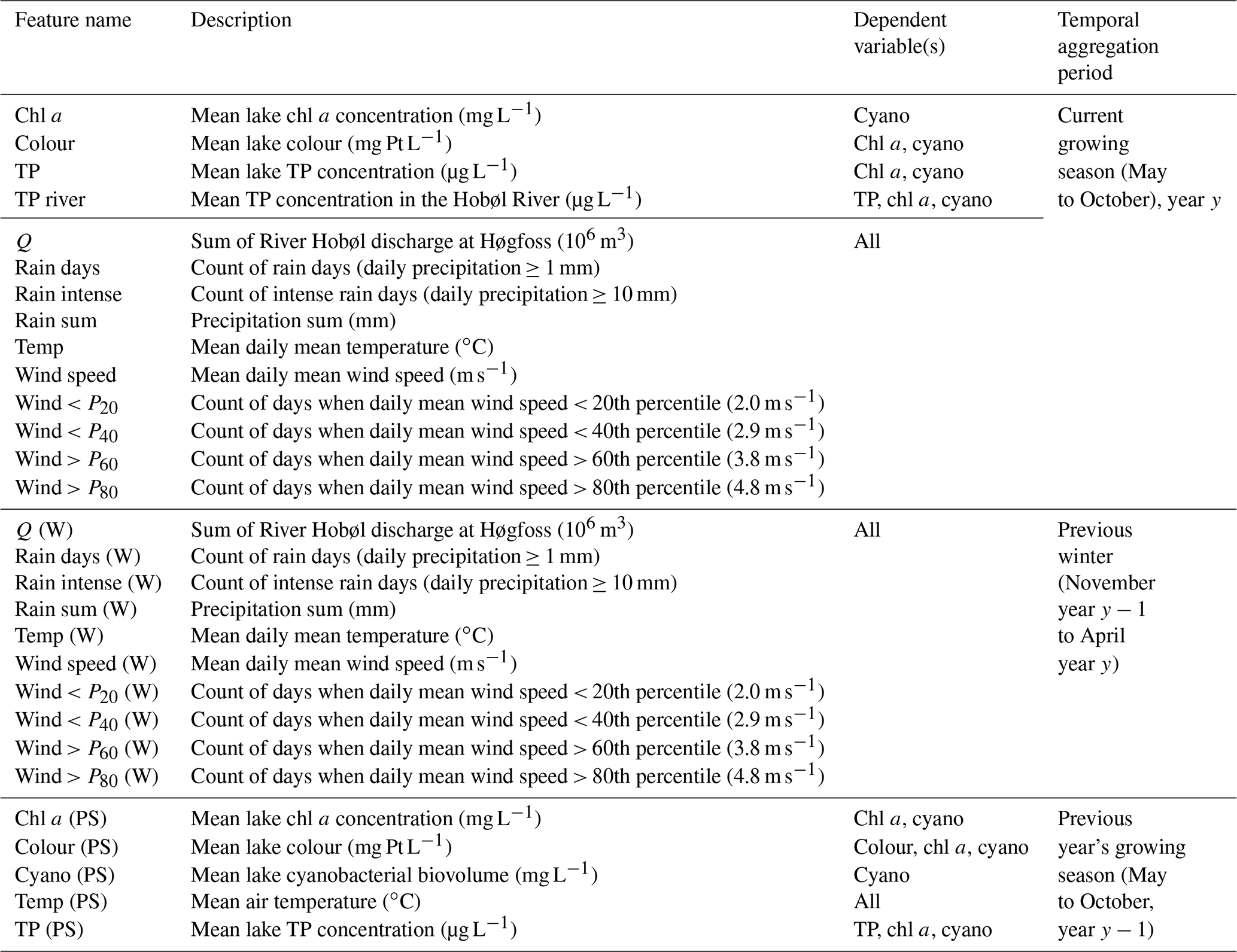
After choosing the variables to include, features were generated for the current May to October growing season, for the previous winter (the November to April 6-month period prior to the current season), and for the previous year's growing season. Overall, we generated up to 29 potential explanatory variables, depending on the response variable (Table 1). Features were derived for the period 1981–2018. Depending on the number of years with missing data, this gave 39 years of data for TP and chl a, 36 for lake colour, and 24 for cyanobacteria.
Table 1Potential explanatory variables (features) considered for each of the four dependent variables (chl a, TP, cyanobacteria, and colour). The temporal aggregation period is given relative to the forecast issue date in spring of the current year, y.
2.5 Feature selection
Having generated a list of potential explanatory variables for each dependent variable, we then carried out exploratory statistical analyses to select the features to include in the GBN, using a combination of the following:
-
Ranked correlation coefficients. As a first screening, we used ranked absolute Pearson's correlation coefficients to highlight potentially important features for each dependent variable.
-
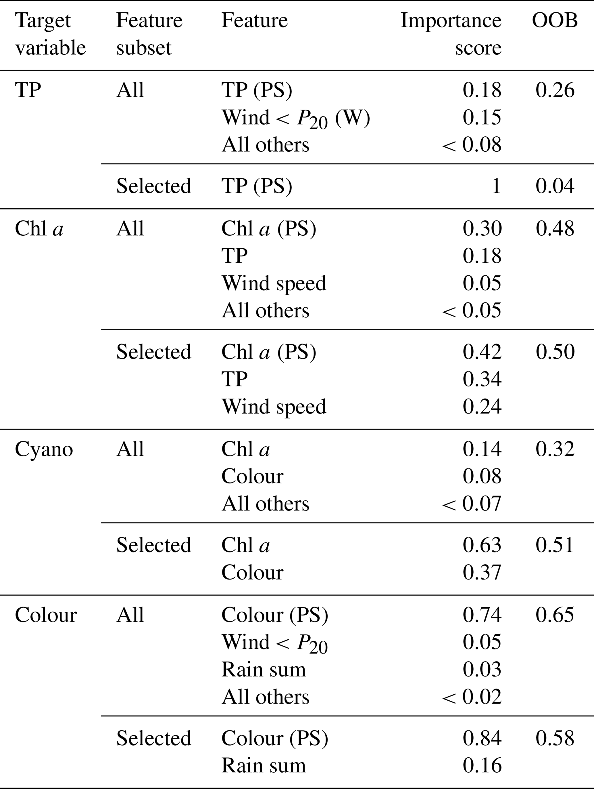
Feature importance. We used a machine learning approach to assess feature importance for each dependent variable, using random forests implemented using the scikit-learn Python package (Pedregosa et al., 2011). Random forests use bootstrapping to partition the data used by each tree, and data not included in each bootstrap sample are used to perform internal validation. We used the out-of-bag (OOB) score and importance scores to rank the feature importance. Random forests have a number of hyperparameters that can be tuned to improve performance. The most important are the number of trees in the forest (n_estimators) and the size of the random subsets of features to consider when splitting a node (max_features). We selected values for these for each dependent variable by plotting the OOB error rate (1 − OOB score) as a function of n_estimators for various choices of max_features.
-
Visual evaluation of relationships. Scatterplot matrices were used for a visual check of whether relationships appeared to be linear and for independence between explanatory variables (required for unconnected nodes in a BN).
-
Process understanding. Finally, we excluded explanatory variables where we did not think there were plausible physical mechanisms underpinning the relationship.
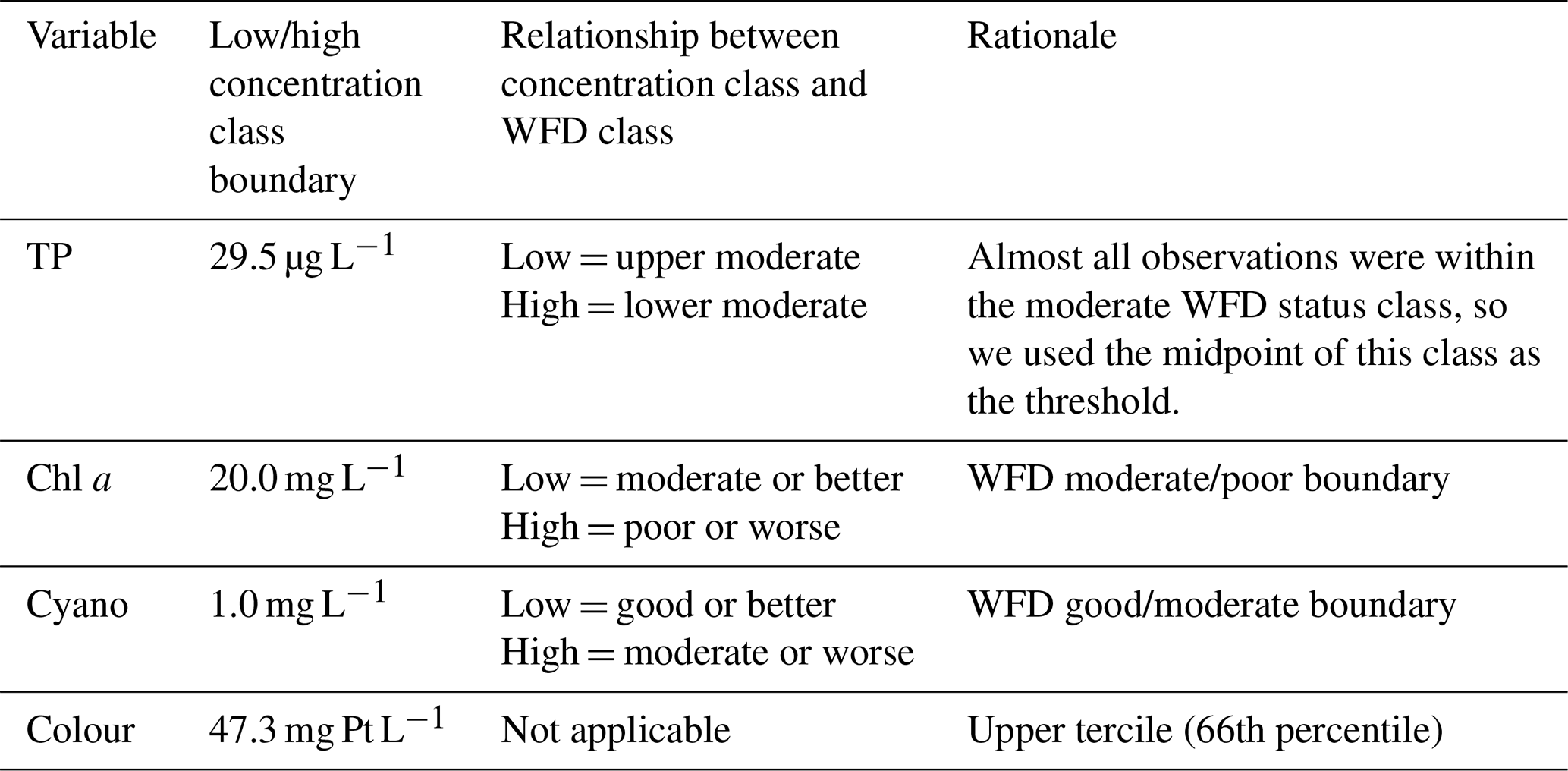
Table 2Management-relevant thresholds used for predicting the probability of lake water quality variables lying within a certain water quality class. The classification is summarised as low concentration (L) and high concentration (H) classes, which translate to a WFD-relevant classification, as described. WFD is the Water Framework Directive.
2.6 Bayesian network development and use in prediction
We first defined the BN structure manually, using the results of the feature selection and process knowledge, to ensure realistic causative relationships between nodes. This structure was then used in both the continuous Gaussian BN and a discrete BN.
2.6.1 Gaussian Bayesian network development
As mentioned in the introduction, Gaussian Bayesian networks (GBNs) are a powerful class of continuous BNs in which all nodes are continuous, and conditional probability distributions (CPDs) are linear Gaussians, which together define a joint Gaussian. Parent nodes therefore have normal distributions with mean μ and variance σ2. Gaussian CPDs of child nodes have a mean which is a linear combination of the parent nodes (with intercept β0 and coefficients βi for each parent node i). To meet the normality requirement of GBNs, we transformed the cyanobacteria data, which were right skewed, by applying a Box–Cox transformation (, with λ=0.1 to give a fairly symmetrical distribution). Predictions for cyanobacteria were then transformed back to the original data scale including bias-adjustment (see Sect. 3.2; Hyndman and Athanasopoulos, 2021). Normality tests were carried out for all variables using scipy.stats (based on D'Agostino and Pearson, 1973). High p values (>0.2) were found for all but lake colour and transformed cyanobacteria (p=0.04 for both). A step change in lake colour is seen around 1998 (Fig. 2), suggesting the distribution of lake colour may be bimodal. The normality assumption was therefore not invalidated at a 1 % significance level but would have been at a 5 % level. Coefficients were then derived for the CPDs at each node using maximum likelihood estimation.
BNs can be used for prediction, our primary aim, by calculating a probability distribution over the variable(s) whose value we would like to know, given the information (evidence) we have about some other variables. Predictions obtained using GBNs contain a mean and a variance, and here, predictions were obtained by averaging likelihood weighting simulations using a subset of nodes as evidence. The predicted value is then the expected value of the conditional distribution. We chose the evidence nodes based on those nodes which could be updated whenever a forecast was produced, using historic data or future forecasts (i.e. observed water quality from the previous summer or forecasted meteorological conditions). As well as predicting absolute values, we also estimated the probability of exceeding a management-relevant threshold for each water quality variable (Table 2).
2.6.2 Discrete Bayesian network development
Finally, we developed a discrete BN for comparison to the GBN. To do this, we first discretised the data, opting for just two classes for most variables given the small sample size. The exception was previous summer's lake colour, for which we used three classes, given a strong relationship between lake colour in the previous and current growing seasons (Sect. 3.1). We used management-relevant thresholds to discretise the current growing season lake TP, chl a, cyanobacteria, and colour (Table 2). For all the other variables (and including lake observations from the previous summer), as we were not constrained by having to discretise into management-relevant classes, we used regression trees to identify the optimal splitting points, to improve the chances of identifying relationships between nodes in the BN. For each dependent variable (TP, chl a, cyanobacteria, and colour), we built a regression tree for each explanatory–dependent variable pair in turn and then used the first or second split point in the tree as the boundary to discretise that explanatory variable (regression trees are in the accompanying GitHub repository; see the code and data availability section). For wind speed, this resulted in highly unbalanced class sizes, so we instead used the median. The chosen boundaries were 31.8 mg L−1 for TP (PS), 16.8 mg L−1 for chl a (PS), 26.8 and 47.3 mg Pt L−1 for colour (PS), 469 mm for rain sum, and 3.55 m s−1 for wind speed. Note that the different discretisation methods used for the current vs. previous year's growing season lake water quality means that the two variables are classified differently, despite having the same underlying data. The resulting classes were relatively well balanced.
We then fitted the conditional probability tables (CPTs) using Bayesian posterior estimation with uniform priors. Including priors helps to avoid overfitting, a common problem with maximum likelihood estimation (mle, where CPTs are fitted just using the relative frequencies), particularly with small sample sizes when the data may not be representative of the underlying distribution. In our case, priors can be thought of as pseudo-state counts added to the actual counts before normalisation. The uniform priors were defined by an imaginary sample size (iss) parameter, whereby the pseudo counts are the equivalent of having observed iss uniform samples of each variable and each parent configuration. The higher the iss, the stronger the effect of the prior on the posterior parameter estimates, while the method becomes mle when iss = 0. The iss parameter thus specifies the weight of the prior compared to the sample and therefore controls the smoothness of the posterior distribution. A common rule of thumb is to use a small non-zero iss to avoid zero entries. However, we experimented with larger values of iss (from 1 to 50) to avoiding overfitting. We did this using a trial-and-error process. During each iteration, we examined the CPTs for spurious relationships and checked the predictive error of the network through cross-validation (see Sect. 2.7.1). We found that an iss of 15 was the smallest value where the majority of unexpected CPT behaviour was smoothed out, while maximising predictive performance.
2.7 BN validation and assessment
We then explored the most appropriate GBN model structure and evaluated the GBN performance using three methods, including (1) cross-validation, carried out on several parts of the network separately and including comparison to the discrete BN, (2) goodness of fit of the whole network compared to observations, and (3) comparison to a simple benchmark model.
2.7.1 Cross-validation of subnetworks
The ability to carry out cross-validation (CV) is a benefit of using bnlearn compared to many graphical BN packages, as it is possible to assess the expected performance of the network for out-of-sample prediction and to compare different models to robustly assess whether certain nodes and arcs are improving the predictive power. Here, we used CV to compare the predictive performance of GBNs with and without meteorological nodes and to compare the GBN and the discrete BN. We used leave-one-out cross-validation, which should produce unbiased skill score estimates even with small sample sizes (e.g. Wong, 2015). In short, the cross-validation was repeated for each predicted node (chl a, cyano, TP, and colour) and involved the following steps: 1 year of data is left out at a time, the BN is fit using the remaining years of data, and then it is used to predict the target node for the left-out year. The procedure is repeated for all years, producing a single time series of predictions. These are then compared to observations to generate skill scores. As the main aim was prediction, we used posterior predictive correlation (reported as R2), mean square error (MSE), and classification error (the proportion of the time the classification was incorrect) as the GBN skill scores and the classification error for the discrete BN. The cross-validation is stochastic and was run for a default 20 times, and the mean skill score was calculated.
Cross-validation requires complete data for all variables and years. For most variables there were few gaps, so we filled up to 1-year gaps by interpolation or backward/forward filling. However, cyanobacteria was only measured from 1996, while other variables were measured from 1980. Rather than dropping all data prior to 1996, which would result in a large loss of training data for TP, chl a, and colour, we instead split the network into a number of smaller networks for the target variables and cross-validated each of these in turn (see Sect. 3.3.1).
2.7.2 Goodness of fit of the whole network
Splitting the BN up into smaller subnetworks is likely to result in a loss of predictive power, so cross-validation could not be used to assess the expected predictive performance of the whole network. Instead, we assessed the performance of the whole network, trained on all data, by simply calculating the goodness of fit of the predictions using the GBN with and without weather nodes. For this, we used correlation, MSE, and classification error, as during cross-validation, and bias (mean of predicted−observed values). We also calculated the Matthews correlation coefficient (MCC) to provide additional information on how well the WFD status class was predicted. MCC is in the range 0 (no skill) to 1 (perfect skill) and has been shown to be a truthful score for evaluating binary classifiers (Chicco and Jurman, 2020). As the training and evaluation data were the same, this may produce an optimistic assessment of model performance.
Table 3Ranked Pearson's correlation coefficients (R) for the four dependent variables (for clarity only are shown). See Table 1 for a description of the variables.

2.7.3 Comparison to a benchmark model
Some extremely simple forecasting methods can be highly effective. As a final test, we compared predictive performance of the GBN to a seasonal naïve forecast (Hyndman and Athanasopoulos, 2021). In this case, the seasonal naïve forecast for the current growing season is simply the observed value from the previous year's growing season.
3.1 Feature selection
For lake TP concentration, key features identified were TP concentration from the previous growing season and, to a lesser extent, wind-related features (Tables 3 and 4). Temporal autocorrelation in lake TP concentration is highly plausible. It is, however, less clear whether the negative correlation with wind speed is causative. We might expect windier conditions to increase sediment resuspension and result in higher TP concentrations (Hanlon, 1999), but higher TP was instead associated with calmer weather (Fig. 3). A positive relationship between the previous summer's TP and winter wind (Fig. 3), together with analyses using monthly aggregated data (Appendix A), suggest that the relationship may not be causative. Wind was therefore not selected for TP.
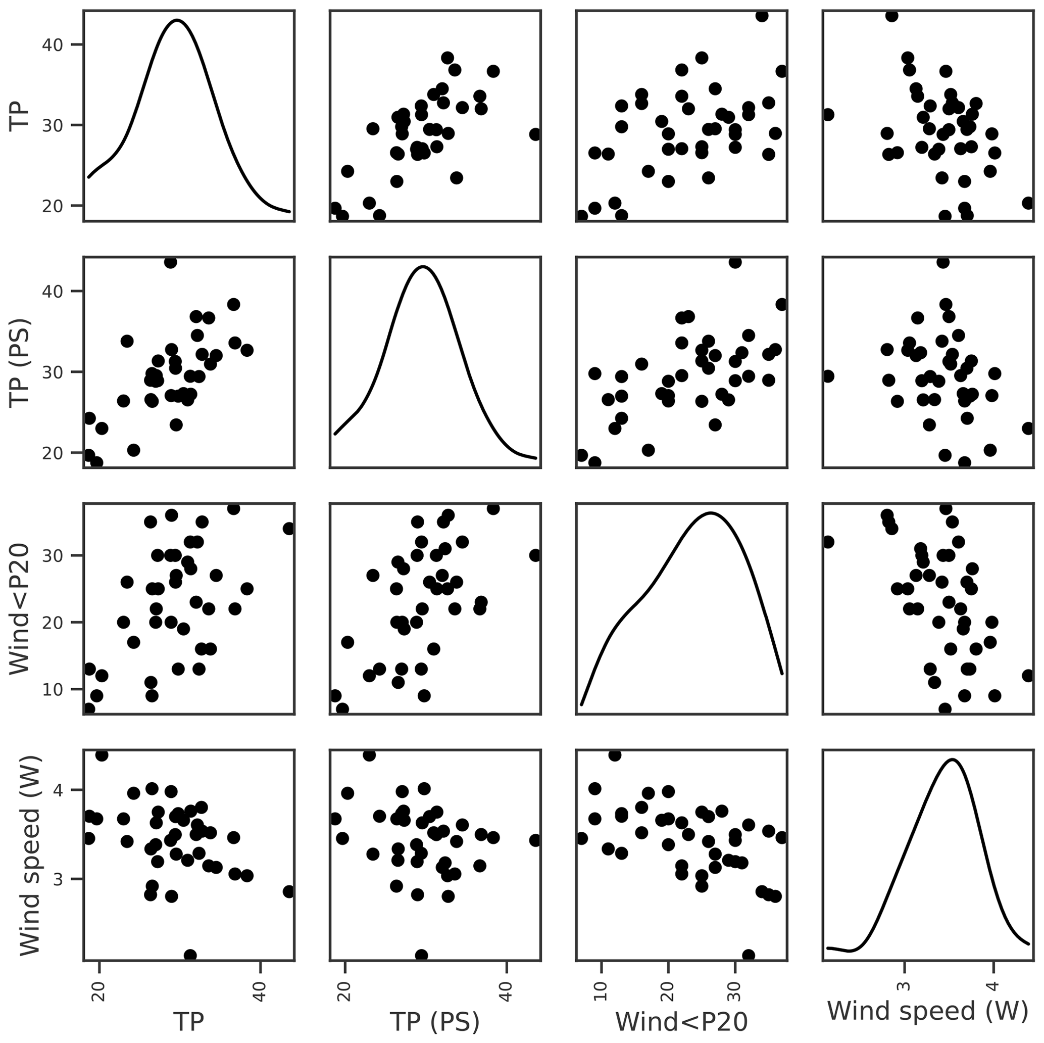
Figure 3Relationships between seasonal mean lake TP concentration and potential explanatory variables of interest, including lake TP from the previous summer (PS), number of days when the daily mean wind speed < 20th percentile (wind < P20), and mean winter (Nov–Apr) wind speed. Density plots estimated using kernel density estimation (kde) are shown along the diagonal.
Table 4Summary of the feature importance analysis for each dependent variable. The out-of-bag (OOB) score gives the overall performance of the random forest regressor model, whilst importance scores rank the importance of the features. Results are shown using all available features (All) and for the feature subset selected for BN development (Selected). See Table 1 for a description of the features.
For chl a, the strongest correlations were with chl a from the previous summer and lake TP concentration (Table 3). Otherwise, the only correlation coefficients above 0.4 were with wind-related features, including a negative relationship with mean wind speed (Fig. 4). This was supported by the feature importance analysis and a model with chl a (PS), lake TP, and wind speed had the highest OOB score (Table 4). There are plausible mechanisms underpinning relationships between these three variables and lake chl a, and all were selected for BN development. In the case of wind, windier weather can cause less stable lake stratification and lower chl a concentrations (Huber et al., 2012; Yang et al., 2016).
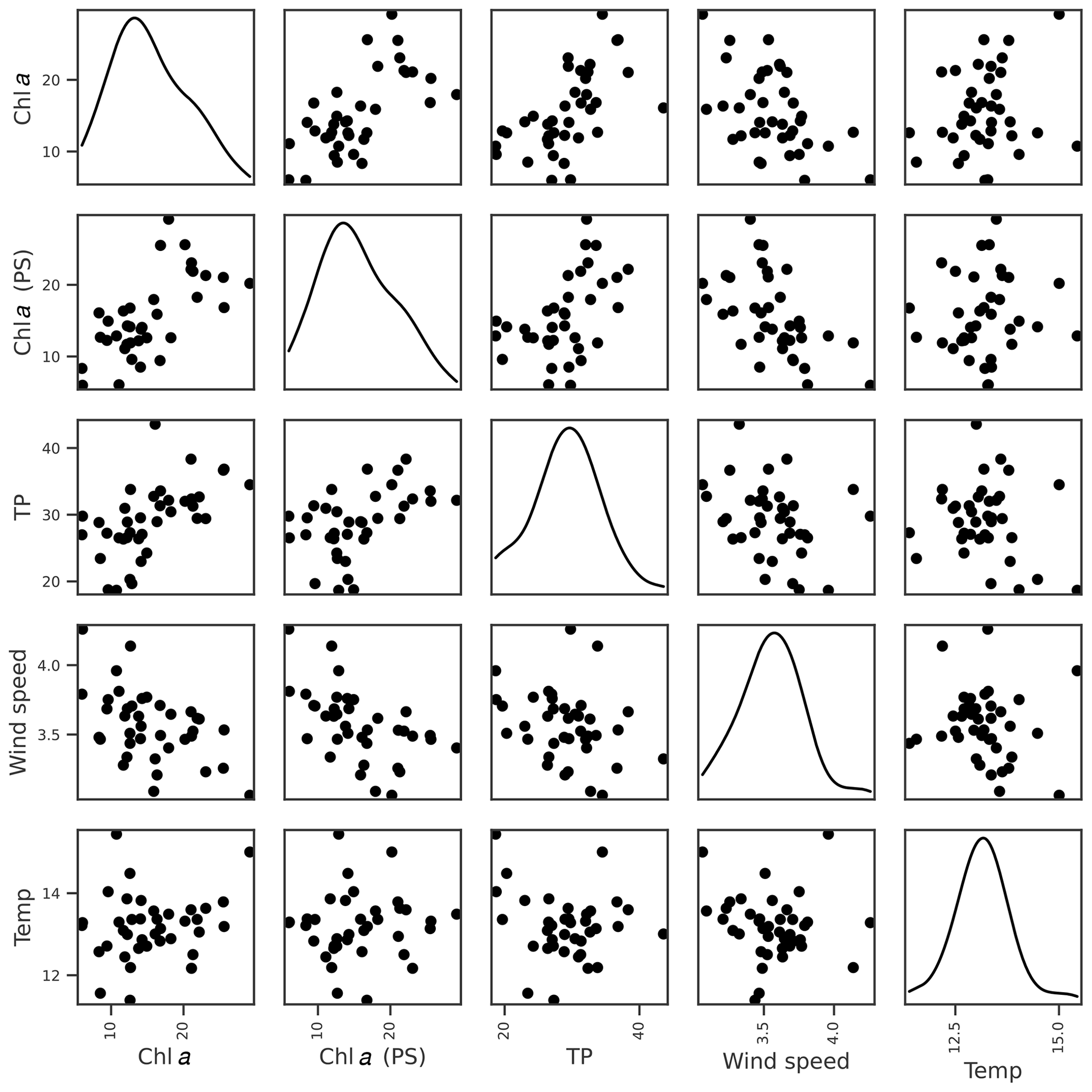
Figure 4Relationships between seasonal mean chl a (mg L−1) and potential explanatory variables of interest, including chl a from the previous summer (PS), seasonal mean TP (µg L−1), wind speed (m s−1), and air temperature (∘C). Density plots estimated using kde are shown along the diagonal.
Air temperature exerted an important control on within-year changes in chl a (Appendix A), but there was no evidence that years with higher summer air temperature were associated with higher mean chl a concentration (Fig. 4).
For cyanobacteria, the strongest correlation was with lake chl a, although a number of other correlations were present (Table 3; Fig. 5). Feature importance analysis also highlighted chl a as being the most important variable (Table 4). Highest OOB values were obtained using just chl a and lake colour, and these were therefore selected as the key explanatory variables for cyanobacteria. The relationship with lake colour is plausible, as an increase in organic matter can affect lake algal communities by reducing the light availability and the availability of nutrients (Nagai et al., 2006), and Senar et al. (2021) found that, above dissolved organic carbon (DOC) concentrations of 8–12 mg L−1, similar to those observed in lake Vanemfjorden (7–10 mg L−1 over the period 1996–2018), cyanobacteria became replaced by mixotrophic species as lake colour increased.
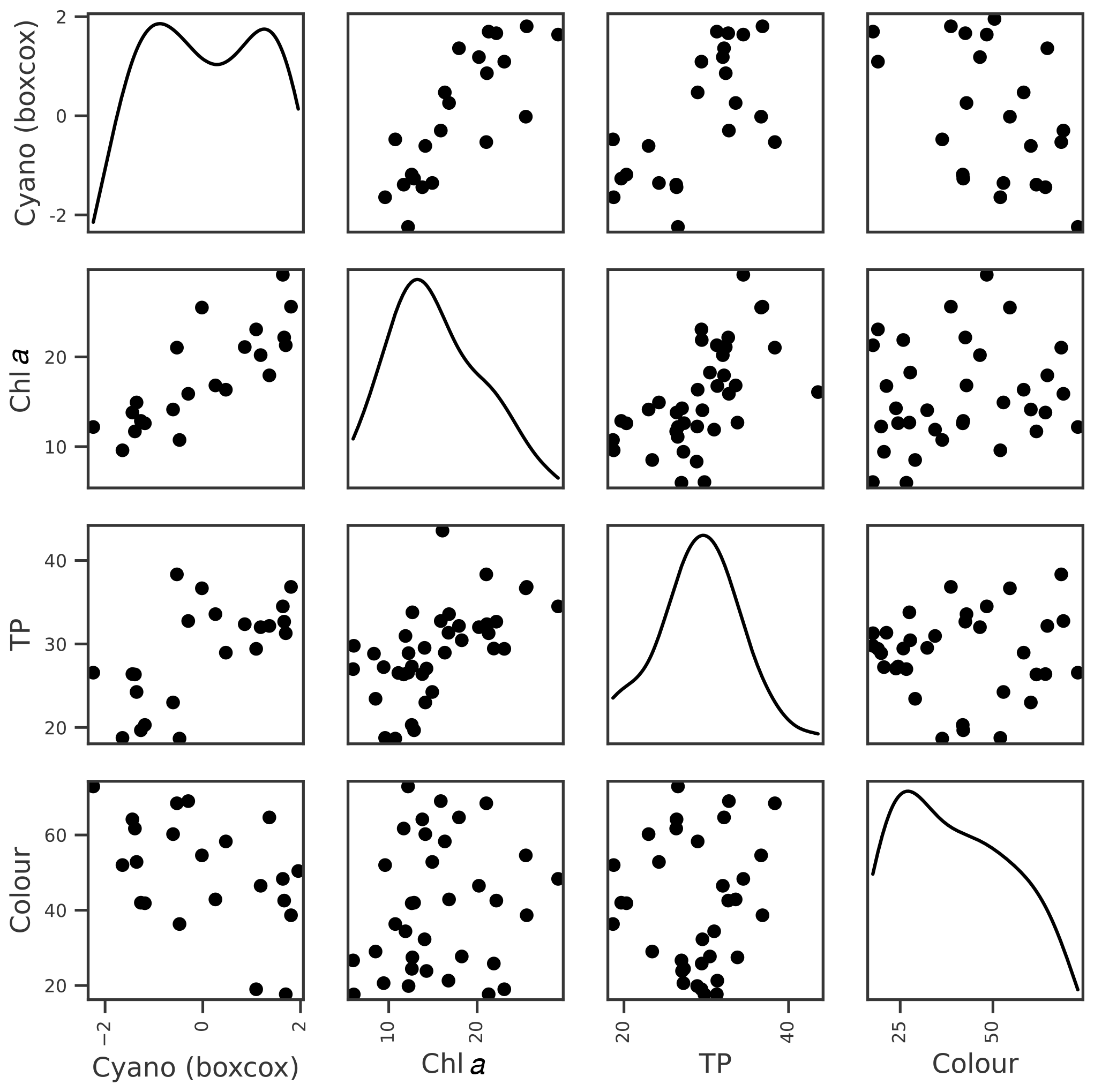
Figure 5Relationships between Box–Cox-transformed seasonal maximum cyanobacteria biovolume and potential explanatory variables of interest, including seasonal means in lake chl a, TP, and colour. Density plots estimated using kde are shown along the diagonal.
Lake colour was very strongly correlated with the previous summer's colour, and probably because of this, the OOB score for lake colour was the highest of all the dependent variables. Colour was also moderately correlated with factors relating to catchment delivery (Table 3; Fig. 6). The three most important features were the previous summer's colour, calm wind days (wind < P20), and rain sum, although the latter two had low importance scores compared to the previous summer's colour (Table 4). As with TP, we suspect that the wind–colour relationship is not causative, as lake colour is relatively uniform throughout the water column in Vansjø, so the impact of wind on lake stratification should be minimal. Wind was therefore dropped, and only the previous summer's colour and rain sum were selected for further BN development.
The findings were relatively robust to the temporal aggregation window, as statistical analyses using a shorter and more causally plausible temporal aggregation resulted in very similar relationships being highlighted (Appendix A). The exception was that higher rainfall and discharge may result in lower cyanobacteria peaks, probably due to flushing, a relationship which was not accounted for in the GBN using 6-monthly aggregation, and a potential area for improvement.
In summary, the following features were selected for BN development for the four target variables:
-
TP – lake TP concentration from the previous summer.
-
Chl a – chl a from the previous summer, lake TP concentration, and wind speed. We also included a relationship between chl a (PS) and TP (PS), as we would not expect these two nodes to be independent.
-
Cyanobacteria – lake chl a and colour.
-
Colour – lake colour from the previous summer and rain sum.
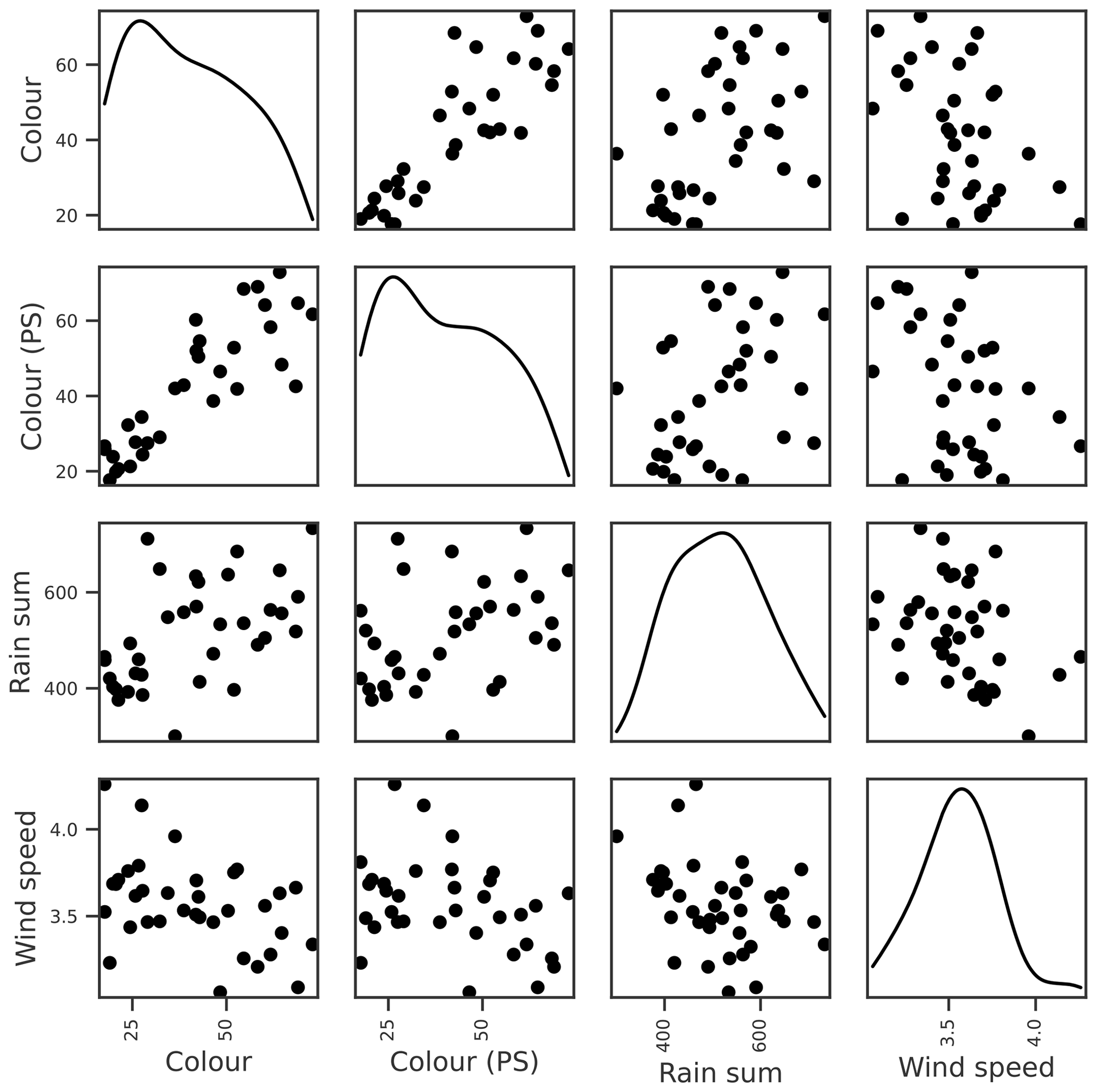
Figure 6Relationships between seasonal mean lake colour and potential explanatory variables of interest, including the colour during the previous summer (PS), seasonal rain sum, and mean wind speed. Density plots estimated using kde are shown along the diagonal.
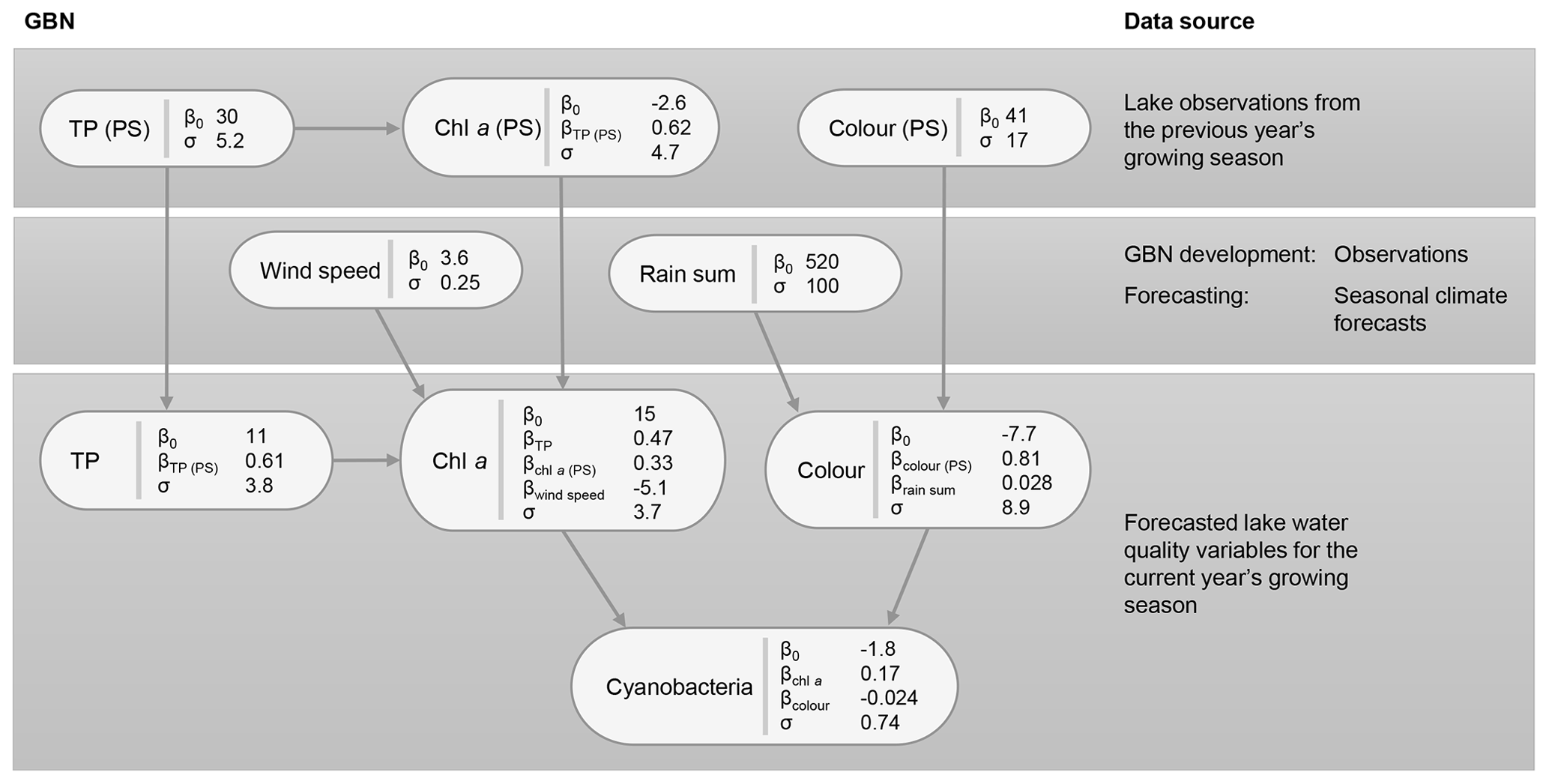
Figure 7Gaussian Bayesian network (GBN) structure and parameters defining the conditional probability densities at each node. Units for standard deviations (σ) and intercepts (β0) are the same as the original data, aside from cyanobacteria, where a Box–Cox transformation was used (λ=0.1). See Table 1 for a detailed description of the variables and Table B1 for 95 % confidence intervals on the fitted coefficients.
3.2 Gaussian Bayesian network development
3.2.1 BN structure and GBN parameters
The key relationships highlighted (Sect. 3.1) were then used to develop the BN structure, which is shown, together with fitted coefficients for the GBN, in Fig. 7. For parentless nodes, coefficients define normal distributions with mean β0 and variance σ2. Child nodes are linear combinations of the parent nodes with intercept β0, coefficients βn, and variance σ2. See Appendix B for 95 % confidence intervals on the fitted coefficients. Fitted coefficients for the GBN were all plausible and matched the simple bivariate relationships between variables seen in the exploratory data analysis.
3.2.2 Fitted discrete BN
The fitted CPTs for the discrete network (Fig. 8) did a slightly more mixed job of representing the relationships between variables. Despite using a relatively high iss value when fitting the network (i.e. giving the priors relatively high weight; see Sect. 2.6.2), several dubious relationships remain in the CPTs. For example, from our exploratory analysis, we expected a negative (or no) wind effect on chl a. However, the opposite effect is seen in the last two rows of the chl a CPT, with an increase in the chance of having high chl a at higher wind speeds. More issues like this were present when a lower iss value was used and are very likely just an artefact due to the small sample size.
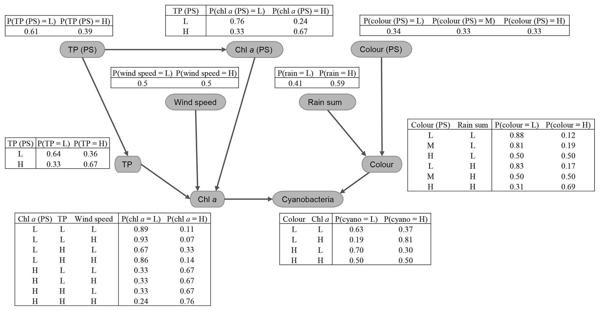
Figure 8Fitted conditional probability tables for the discrete Bayesian network. Values were discretised into low (L) or high (H) classes – a medium (M) class was also included for colour (PS) – as described in Sect. 2.6.2.
3.3 GBN validation and assessment
We then explored the most appropriate GBN model structure and assessed its predictive performance using the following: (1) cross-validation using subsets of the GBN, including a comparison to the discrete BN, (2) goodness of fit of the whole network compared to observations, and (3) a comparison to a simple benchmark model.
3.3.1 Cross-validation using subsets of the network
As mentioned in Sect. 2.7, cross-validation (CV) requires complete data for all variables and years. As cyanobacteria has only been monitored since 1996, to avoid a large loss of data for TP, chl a, and colour, we split the GBN up into smaller subnetworks before performing cross-validation for each target node separately, as follows.
-
TP and chl a – drop cyanobacteria, colour, the previous summer's colour, and rain nodes from the BN and use the whole 1981–2018 period in cross-validation.
-
Colour – as colour was linked to the network through cyanobacteria, to be able to include the full period 1981–2018 we had to drop all nodes, aside from colour and its parents (rain sum and the previous summer's colour).
-
Cyanobacteria – the whole network was used but only with data from 1997.
CV results comparing the classification error of the GBN and the discrete BN are shown in Table 5. We might expect the discrete BN, which was fit to discrete data, to do a better job of predicting the water quality class than the GBN. However, this was only the case for chl a. The discrete network was a worse classifier than the GBN for colour and performed similarly for cyanobacteria and TP.
Table 5Mean predictive performance of different Bayesian network (BN) structures, including the Gaussian Bayesian network (GBN) with and without weather nodes and a discrete BN, assessed through cross-validation. The BNs used for each variable were subsets of the BN shown in Fig. 7, for all but cyanobacteria, to make the most of all available data (see Sect. 3.3.1). GBN cyanobacteria predictions were back-transformed to the original data scale before calculating statistics (see Sect. 2.6.1). Note: RMSE is root mean square error; n/a is not applicable.

Predictive performance of the GBN with and without weather nodes is also shown in Table 5. Lake colour was the only variable for which model performance was a little better when meteorological variables were included, although the gains were marginal. For chl a and TP, performance was near-identical with or without weather nodes, while it was slightly worse for cyanobacteria when weather nodes were included. Further investigation showed that this was due to the wind–chl a arc. Overall, CV results suggest a marginal benefit to using rain sum when predicting lake colour but that wind should be dropped from the GBN.
3.3.2 Goodness-of-fit of the whole network
Model performance of the whole network, using the same data for both fitting and assessment, is shown in Table 6. Performance was best for lake colour (R2>0.7), which showed particularly high temporal autocorrelation. The same general lack of sensitivity to weather nodes was seen as in the CV results and when considering additional model performance statistics (Table 6; Fig. 9).
Table 6Performance of the GBN, with and without weather nodes, fit using the whole historic period (no cross-validation) and the whole BN. Performance of the seasonal naïve forecast is also shown. The MCC and classification error reflect classifier skill, while other statistics reflect how well the mean predicted values match observations. Note: RMSE is root mean square error; MCC is Matthews correlation coefficient.
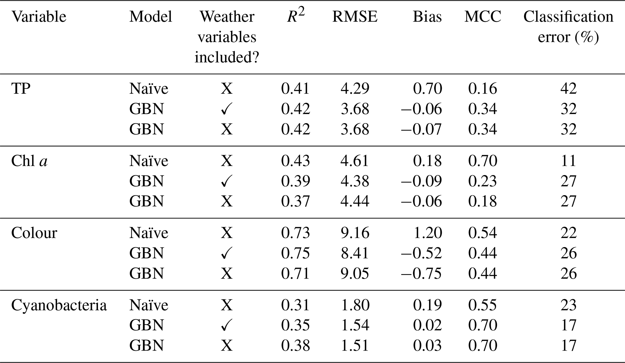
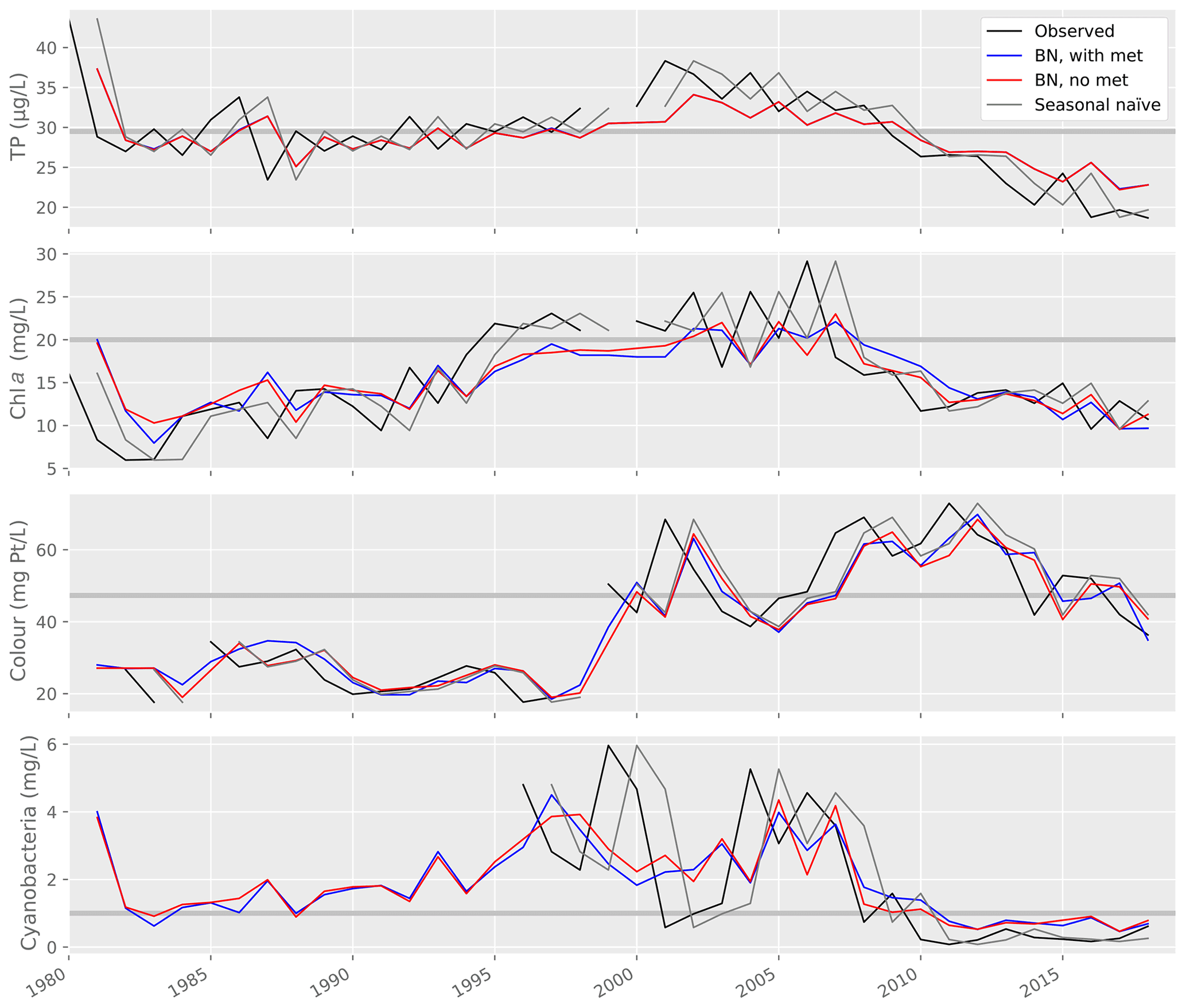
Figure 9Lake water quality observations and predictions from a range of models, including the Gaussian Bayesian network (BN) with and without weather variables, and a seasonal naïve forecast. Horizontal grey lines show the thresholds used to classify predictions into two WFD-relevant classes (see Table 2).
3.3.3 GBN predictions compared to a benchmark model
Model performance was then compared to the performance of a seasonal naïve forecaster (Table 6; Fig. 9). For TP and cyanobacteria, the GBN performed better than the naïve forecast for all statistics. For lake colour, the GBN performed better at all but classification. For chl a, the naïve forecast performed slightly better. It was particularly better at classification and, from an inspection of Fig. 9, this is likely because the GBN predictions often happen to lie slightly under the 20 mg L−1 threshold used in the classification.
3.4 Forecasting to support water management
An example of a prototype seasonal forecast is available at https://watexr.data.niva.no/ (last access: 22 April 2022). The forecast includes the probability of being in one of two WFD-relevant status classes, the expected (mean) value, some historic skill information, and a text summary to aid in the interpretation of the forecast (e.g. chl a is expected to be moderate or better. Confidence level: medium). The forecast's layout was developed together with the regional water manager (Morsa) to ensure that it met their needs, and they have expressed optimism about the use of these kinds of forecasts to support water management and have identified actions which could be taken based on reliable-enough forecasts (Jackson-Blake et al., 2022). As well as providing an easy way of deriving probabilistic forecasts, we found a real benefit of using BNs for forecasting was in stakeholder engagement and model co-development. We found that the easy and transparent visualisation of the model increased stakeholder engagement in the model development process and stakeholders' ability to correctly interpret the probabilistic predictions (Jackson-Blake et al., 2022).
The main aims of this study were (1) to develop a model for seasonal forecasting of lake water quality and (2) to demonstrate the use of a continuous GBN for environmental modelling over more traditional discrete BN approaches. We discuss each of these in turn below.
4.1 Seasonal forecasting of lake water quality
4.1.1 Drivers of interannual variability in lake water quality
In Vansjø, key water quality predictors were values observed during the previous summer. Indeed, for lake TP concentration, this was the only predictor variable selected (Sect. 3.1). The strength of this annual autocorrelation, together with relatively low interannual variability in lake water quality (Fig. 9), are likely the reasons why the seasonal naïve forecast performed only slightly worse than the GBN and even slightly better for chl a (Sect. 3.3.3). Aside from high temporal autocorrelation, we found positive relationships between lake TP concentration and chl a and cyanobacteria, as widely documented elsewhere (Rousso et al., 2020). We also found evidence for a decrease in cyanobacteria as lake colour increased, again a previously documented effect (Sect. 3.1). No link was seen between lake colour and chl a, however, perhaps due to quality issues with the colour data before 1998 (Sect. 2.3), while cyanobacteria data were only available from 1996 and so missed the colour step change. Although we found some evidence for relationships between weather variables and water quality, subsequent analyses suggested that it was not worth including weather nodes in the GBN, as the improvements in predictive performance were marginal (for lake colour) or absent (Sect. 3.3), and it is highly unlikely that the marginal improvements would still be seen after replacing real observed historical meteorological data with seasonal climate model hindcasts.
The lack of a temperature effect on algal biomass or cyanobacteria is interesting, as we might expect warmer summers to be accompanied by more intense blooms. However, the results fit with a number of studies which found that warming effects were minor compared to nutrient effects (Lürling et al., 2018; Robarts and Zohary, 1987) and that water column stability was a key driver of cyanobacteria dynamics in dimictic lakes (Taranu et al., 2012), with wind playing a more dominant role than seasonal air temperature (Huber et al., 2012; Yang et al., 2016). We did, however, find a strong air temperature effect on the within-year variation in chl a and, to a lesser extent, cyanobacteria (Appendix A), likely because the within-year variability is large compared to intra-annual variability and follows a systematic seasonal pattern. When looking in more detail at some of the BN studies in which relationships were identified between air temperature and algal variables (Shan et al., 2019; Rigosi et al., 2015; Williams and Cole, 2013; Moe et al., 2019; Couture et al., 2018), the observations used to fit the BN were not annually aggregated, so both with- and between-year variability were included. This may be appropriate if the aim is to look at algal dynamics within a year. However, it may not be appropriate for predicting interannual variation or for longer-term prognoses. Although temperature is likely to be important in many areas, it seems likely that a number of studies will have overestimated its importance by assuming that within-year relationships between temperature and algal dynamics can be used to infer future algal responses to increases in summer temperature under climate change.
4.1.2 Operational forecasting using seasonal climate forecasting
One of the original aims of the study was to explore whether the latest seasonal climate forecasting products could be used to support water management by enabling improved seasonal water quality forecasting. However, as we did not find a strong sensitivity to seasonal climate, this aim became redundant. In systems which are more sensitive to seasonal climate, a next step would be to assess GBN predictive performance using seasonal climate model hindcasts when making predictions (as in Mercado-Bettín et al., 2021). A comparison of model forecasting skill using seasonal climate model hindcasts versus observed weather would then allow for an assessment of the value of seasonal climate model hindcasts. Seasonal climate forecasts are probabilistic and should only be used to give a broad indication of the likely direction of change, often in terms of tercile probabilities (e.g. there is a 60 % chance that next summer will be windier than normal). A hybrid BN would therefore be a good option, with discrete nodes for the seasonal climate variables.
4.1.3 Data limitations and potential for improvement
As with all data-driven models, the quality of our model strongly relies on the availability and quality of the data. In this regard, we see potential for a number of improvements, as follows:
-
Although the lake has a long history of monitoring, the training dataset is very small for a data-driven model (≤39 data points). The lake showed low interannual variability, with gradual changes over time and few extreme events. Statistical power in a multivariate analysis is therefore limited.
-
Peaks in cyanobacteria were defined by a single point, as in WFD classification, using relatively low-frequency monitoring. An improvement would be for this value to be calculated more robustly, from the mean of a number of consecutive highest points, for example.
-
We only used data from a single point in the lake, while lake water quality can have high spatial variability. In Vanemfjorden, for example, there were bathing bans in place from 2000–2007, and yet the cyanobacteria observations from the monitoring point are not particularly high during this period. Remote sensing products could help address this issue and are increasingly being used in cyanobacteria bloom prediction (Bertani et al., 2017; Stumpf et al., 2012).
Overall, our GBN predictions are almost entirely reliant on conditions observed during the previous summer. Despite the short residence time of the lake, if TP concentrations are buffered by lake sediment P release, seasonal algal peaks are not temperature-limited, and water column stability is relatively insensitive to seasonal wind and temperature (because the water column is regularly mixed, for example), then this rather simple model may be appropriate. All these things are plausible in this shallow lake with a long history of eutrophication. However, it is also likely that our model was limited by the underlying data, as mentioned above, and, for cyanobacteria, by the 6-month temporal aggregation window used (see Appendix A). As an example of a limitation of the model, conditions during the previous winter are not taken into account when making forecasts. However, there is a general consensus that flooding in winter 2000–2001 caused a large input of TP to the lake and was responsible for the cyanobacterial blooms that occurred in subsequent years (Haande et al., 2011). Our bottom-up approach to selecting variables to include in the model meant that, as we did not find a relationship between winter discharge and lake TP concentration, it was not included. While this bottom-up approach ensures that the model is not affected by preconceived (but potentially incorrect) beliefs, it also means that rarely observed, but perhaps important, relationships are not included. In this case, incorporating expert knowledge (to decide on additional nodes to include in the BN and on CPD coefficients) could increase the robustness of the BN at predicting out-of-sample conditions, particularly the impact of extreme events. An alternative, albeit more time-consuming approach, could be to include process-based model simulations to increase the size of the training data, assuming a robust model could be set up. The BN could then be used as a metamodel, as has been done previously at the site in the context of longer-term climate and land use change studies (Moe et al., 2019; Couture et al., 2018). However, process-based lake models typically only predict chl a, so cyanobacteria forecasts would still rely on data-derived empirical relationships or expert knowledge.
4.2 Continuous GBNs for environmental prediction
With GBNs, it is straightforward to produce probabilistic predictions for water quality variables of interest. Predicting the probability of reaching a management target, such as a specific WFD status class, is also straightforward and of direct management relevance (Sect. 3.4), and, although not demonstrated here, it is easy to update the training dataset using new data. These features make the approach well suited to forecasting. In terms of performance, our GBN was modest in its prediction abilities. As discussed above, the performance was likely limited by the nature of the lake and the data available for training, but we believe the approach itself was highly promising and would likely result in a more powerful forecasting tool in lakes or rivers which showed higher interannual variability and sensitivity to seasonal discharge and climate or if used for forecasting at shorter timescales (daily or monthly, for example).
We found that perhaps one of the main benefits of using a GBN over a discrete BN was the speed with which a sensible network could be developed. Our GBN parameters could be easily fit in a physically plausible way using only observed data, despite the small dataset. Developing a comparable discrete BN was a much more subjective and time-consuming process, both in terms of the discretisation of the data and also deciding on the weighting of the uniform prior to try to ensure sensible CPTs (Sect. 2.6.2).
However, the GBN approach has limitations which may be problematic in some settings. The normality assumption may not be appropriate, nor may it be appropriate to assume linear relationships between variables. Although there was no clear evidence for nonlinear relationships (Sect. 3.1), they are common in ecological pressure response relationships, including cyanobacteria blooms (Solheim et al., 2008). Overall, better performance might have been achieved with less stringent parametric requirements. Nonparametric or semi-parametric BN development has received considerable attention in recent years (Marcot and Penman, 2019), with a number of promising developments (e.g. Masmoudi and Masmoudi, 2019; Boukabour and Masmoudi, 2020; Hanea et al., 2015), and we expect that nonparametric continuous BN algorithms will increasingly become available in commonly used BN software. However, the simplicity of the normal approximation used in GBNs means they are likely to remain a good first choice. For people who use BN software that cannot handle continuous nodes, a good alternative could be to make use of commonly available functionality which allows the user to specify a continuous probability distribution for a node, which is then discretised within the software.
GBNs have much in common with multiple linear regression (MLR), where linear relationships and Gaussian error distributions are usually assumed and which are also able to produce probabilistic predictions of continuous variables. Indeed, the local distributions in a GBN are ordinary least squares regressions, i.e. univariate MLR involving only root nodes that are ancestors of the output. Both GBN and MLR approaches have advantages and disadvantages when it comes to environmental modelling and forecasting. MLR models have the advantage that input datasets do not need to be normally distributed, and they are typically easy to implement with standard software. MLR has been successfully applied to algal bloom forecasting in Lake Erie, for example (Ho and Michalak, 2017). The benefits of the BN approach include, for example, the ease of predicting multiple explanatory variables, as was the focus here, where the interest was in forecasting more than just algal bloom risk. Indeed, perhaps the main strength of using a GBN over MLR is that GBNs provide a powerful visual representation of potentially complex interdependencies between variables. By providing a convenient way of defining and visualising a multivariate model, it becomes easier to explicitly incorporate domain knowledge into the model building process (such as which variables affect which other variables) and facilitate collaborative model development and communication of results (Sect. 3.4). Based on our experience in this study, we believe that the process of constructing a GBN forces modellers to think about key relationships and to consider more carefully common MLR pitfalls such as multicollinearity and omitted variable bias.
We developed a continuous GBN to produce probabilistic forecasts for average growing season (May–October) lake water quality (TP, chl a, and colour) and maximum cyanobacteria biovolume. The aim was to provide early warning, in the spring of a given year, of the likely conditions for the coming season. This is, to our knowledge, one of the first continuous GBNs for water quality prediction and one of few continuous BNs in environmental modelling more generally. Overall, we found the GBN approach to be well suited to seasonal water quality forecasting. It is straightforward to produce probabilistic predictions, including the probability of lying within a WFD-relevant status class. The process of developing the GBN was substantially less time-consuming and subjective than developing a discrete BN, and the GBN could be sensibly parameterised just using observed data, despite the small dataset. Despite the parametric constraints of GBNs, their simplicity, together with the relative accessibility of BN software which includes GBN handling, means they are a good first choice for BN development, which we think should be considered more widely when data are continuous.
Although the GBN approach itself proved to be promising, we had more mixed success with forecasting seasonal (or interannual) lake water quality at our study site. Although our exploratory data analysis suggested that wind and precipitation exerted a control on interannual variability in lake water quality, these relationships were weak, and overall our lake showed low sensitivity to seasonal climate. Instead, the dominant source of predictability was simply the lake water quality observed the previous year. Because of this strong inertia, the GBN did not perform much better than a naïve seasonal forecast. Potential improvements, which could make the model more powerful at predicting seasonal water quality, include incorporating expert knowledge on the likely impacts of rare events into the BN structure and conditional probabilities, improving the quality of the training data, and expanding the training set using synthetic process-based model results. We found a much stronger weather control on within-year variability in lake water quality, and we envisage a more management-relevant forecasting tool could be developed by adapting the approach to forecast water quality at subannual timescales or by applying it to forecast seasonal water quality of water bodies (rivers or lakes) that show higher interannual variability and sensitivity to seasonal climate.
A1 Method
Temporal aggregation over the whole growing season is coarse and may miss causative relationships. We therefore also carried out finer-scale aggregation to check and expand on the results obtained from the 6-monthly analyses. This finer-scale aggregation included the following:
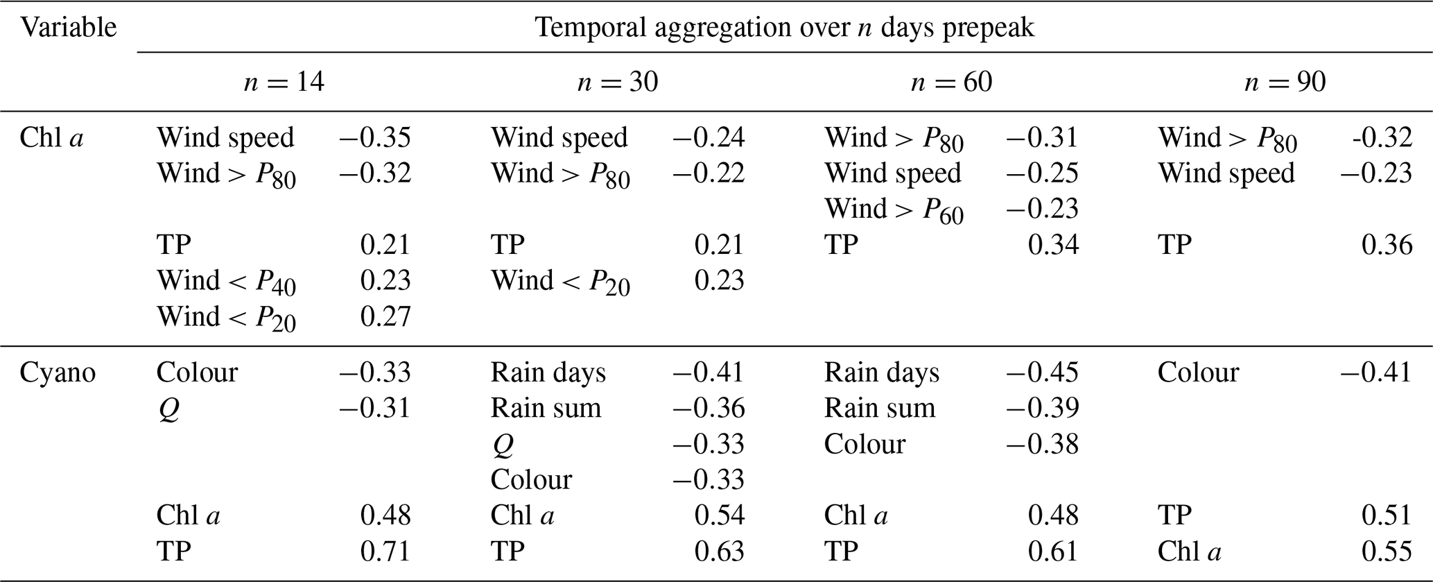
Table A1Pearson's R correlation coefficients for seasonal maxima of chl a and cyanobacteria and potential explanatory variables aggregated (mean or sum) over n days before the algal peak occurred. For clarity, only are shown for chl a and for cyanobacteria.
-
Algal peaks and prepeak conditions for explanatory variables. For each year, we selected peak (maximum) values for chl a and cyanobacteria. We then calculated, for chl a and cyanobacteria in turn, the means or sums of the potential explanatory variables over 14, 30, 60, and 90 d prepeak. By ensuring that the potential explanatory variables only include data from before the observed algal peak, this aggregation method should have more power to identify causative relationships, while still focusing on interannual variation.
-
Monthly aggregation. A repeat of the exploratory statistical analysis (Sect. 2.5) using monthly data to explore the causes of both within- and between-year variability.
A2 Results
A2.1 Algal peaks and prepeak conditions for the explanatory variables
For chl a, the strongest relationships were seen with lake TP concentration and wind-related variables (Table A1), as in the analysis using 6-monthly aggregation. For cyanobacteria, the strongest correlations were with lake TP and chl a concentrations, and there was also a relationship with lake colour, as in the 6-monthly analysis. In contrast to the whole-season analysis, relationships between cyanobacteria and variables relating to wetness and flow were seen for some temporal aggregation windows, suggesting that the larger the rainfall and river discharge (and the shorter the lake water residence time) over the preceding 30–60 d, the lower the cyanobacterial biomass. Overall, this analysis, using a shorter and more causally plausible temporal aggregation, resulted in very similar features being selected as in the whole-season aggregation, with the exception that hydrology and residence time may play more of a role in cyanobacteria bloom development.
A2.2 Monthly aggregation
For all variables, the strongest relationships were with the values observed in the previous month(s), and there were strong correlations between values observed in the previous summer. As well as this strong temporal auto-correlation, potentially important relationships included the following:
-
TP. The strongest correlations were with the previous summer's TP (R=0.45), and there were weaker correlations with wind. For example, the calmer the previous winter or 2–6 months, the higher the TP (R≤0.31, depending on the lag), and the windier the previous winter or 6 months, the lower the TP (, depending on the lag). Stronger correlations were seen between TP and wind over the previous ≥2 months rather than the previous or current month. Wind should have an immediate and relatively short-lived effect on TP via water column mixing, so this suggests that the relationship is not causative. Correlations with all other variables were weak ().
-
Chl a. The strongest correlations were with the current month's air temperature (R=0.50) and the air temperature in previous months. Correlations with all other variables were weaker ().
-
Cyanobacteria. The strongest correlations were with chl a concentration (R=0.71), lake colour (), lake TP concentration (R=0.41), the previous summer's cyanobacteria and TP concentrations (R=0.39 and R=0.37, respectively), and winter wind (R=0.36 or lower, depending on the wind percentile).
-
Colour. The strongest correlations were with the previous summer's colour (R=0.72) and with rain variables, particularly with the precipitation sum and the number of intense rain days over the previous 5 or 6 months (R in the range 0.56–0.60) and with discharge sum the previous 3 months (R=0.54). There was also a negative correlation with air temperature in the current or previous 1–3 months (R in the range −0.51 to −0.44). All other correlations had .
Overall, many of the same variables which were important in explaining interannual differences were highlighted as being important. However, a key difference is the appearance of a strong correlation between air temperature and chl a concentration, discussed further in Sect. 4.1.1.

Data and scripts are available at https://github.com/LeahJB/gbn-vansjo (Jackson-Blake, 2022a), and the first release (v0.1) of the repository is archived at https://doi.org/10.5281/zenodo.6535592 (Jackson-Blake, 2022b).
LJB conceptualised and carried out the analysis, with input on limnological process understanding from SH, SJM, and FC, on Bayesian network development from SJM, and with machine learning and Python/R integration support from JES. LJB prepared the paper, with contributions from all co-authors.
The contact author has declared that neither they nor their co-authors have any competing interests.
Publisher's note: Copernicus Publications remains neutral with regard to jurisdictional claims in published maps and institutional affiliations.
This article is part of the special issue “Frontiers in the application of Bayesian approaches in water quality modelling”. It is a result of the EGU General Assembly 2020, 3–8 May 2020.
Many thanks to the whole WATExR project team, for fruitful collaboration and discussions on the topic of seasonal forecasting and method development. Thanks also to José-Luis Guerrero, for assisting in sourcing the meteorological data.
This work has been carried out as part of the WATExR project, part of ERA4CS, an ERA-NET initiated by JPI Climate. The work has been funded by the Research Council of Norway (project no. 274208), with co-funding by the European Union (grant no. 690462).
This paper was edited by Ibrahim Alameddine and reviewed by two anonymous referees.
Aguilera, P. A., Fernández, A., Fernández, R., Rumí, R., and Salmerón, A.: Bayesian networks in environmental modelling, Environ. Model. Softw., 26, 1376–1388, https://doi.org/10.1016/j.envsoft.2011.06.004, 2011.
Barton, D. N., Saloranta, T., Moe, S. J., Eggestad, H. O., and Kuikka, S.: Bayesian belief networks as a meta-modelling tool in integrated river basin management – Pros and cons in evaluating nutrient abatement decisions under uncertainty in a Norwegian river basin, Ecol. Econ., 66, 91–104, https://doi.org/10.1016/j.ecolecon.2008.02.012, 2008.
Bergström, A.-K. and Karlsson, J.: Light and nutrient control phytoplankton biomass responses to global change in northern lakes, Global Change Biol., 25, 2021–2029, https://doi.org/10.1111/gcb.14623, 2019.
Bertani, I., Steger, C. E., Obenour, D. R., Fahnenstiel, G. L., Bridgeman, T. B., Johengen, T. H., Sayers, M. J., Shuchman, R. A., and Scavia, D.: Tracking cyanobacteria blooms: Do different monitoring approaches tell the same story?, Sci. Total Environ., 575, 294–308, 2017.
Boukabour, S. and Masmoudi, A.: Semiparametric Bayesian networks for continuous data, in: Communications in Statistics – Theory and Methods, Taylor & Francis, 1–23, https://doi.org/10.1080/03610926.2020.1738486, 2020.
Bruno Soares, M. and Dessai, S.: Barriers and enablers to the use of seasonal climate forecasts amongst organisations in Europe, Climatic Change, 137, 89–103, https://doi.org/10.1007/s10584-016-1671-8, 2016.
Carpenter, S. R., Cole, J. J., Kitchell, J. F., and Pace, M. L.: Impact of dissolved organic carbon, phosphorus, and grazing on phytoplankton biomass and production in experimental lakes, Limnol. Oceanogr., 43, 73-80, https://doi.org/10.4319/lo.1998.43.1.0073, 1998.
Chicco, D. and Jurman, G.: The advantages of the Matthews correlation coefficient (MCC) over F1 score and accuracy in binary classification evaluation, BMC Genom., 21, 1–13, 2020.
Couture, R.-M., Tominaga, K., Starrfelt, J., Moe, S. J., Kaste, Ø., and Wright, R. F.: Modelling phosphorus loading and algal blooms in a Nordic agricultural catchment-lake system under changing land-use and climate, Environ. Sci.: Proc. Imp., 16, 1588–1599, 2014.
Couture, R.-M., Moe, S. J., Lin, Y., Kaste, Ø., Haande, S., and Solheim, A. L.: Simulating water quality and ecological status of Lake Vansjø, Norway, under land-use and climate change by linking process-oriented models with a Bayesian network, Sci. Total Environ., 621, 713–724, 2018.
D'Agostino, R. and Pearson, E. S.: Tests for departure from normality. Empirical results for the distributions of b2 and , Biometrika, 60, 613–622, 1973.
de Wit, H. A., Valinia, S., Weyhenmeyer, G. A., Futter, M. N., Kortelainen, P., Austnes, K., Hessen, D. O., Räike, A., Laudon, H., and Vuorenmaa, J.: Current browning of surface waters will be further promoted by wetter climate, Environ. Sci. Technol. Lett., 3, 430–435, 2016.
Direktoratsgruppen Vanndirektivet: Klassifisering av miljøtilstand i vann, 222, https://www.vannportalen.no/veiledere/klassifiseringsveileder/ (last access: 10 May 2022), 2018.
Dudgeon, D., Arthington, A. H., Gessner, M. O., Kawabata, Z.-I., Knowler, D. J., Lévêque, C., Naiman, R. J., Prieur-Richard, A.-H., Soto, D., and Stiassny, M. L.: Freshwater biodiversity: importance, threats, status and conservation challenges, Biol. Rev., 81, 163–182, 2006.
ECOSTAT: Common implementation strategy for the Water Framework Directive (2000/60/EC), Guidance document no. 13: Overall approach to the classification of ecological status and ecological potential, Office for Official Publications of the European Communities, Luxembourg, 53 pp., https://circabc.europa.eu/sd/a/06480e87-27a6-41e6-b165-0581c2b046ad/Guidance No 13 - Classification of Ecological Status (WGA).pdf (last access: 9 June 2022), 2005.
Geiger, D. and Heckerman, D.: Learning Gaussian Networks, in: Uncertainty Proceedings 1994, Elsevier, 235–243, https://doi.org/10.1016/B978-1-55860-332-5.50035-3, 1994.
Gozlan, R., Karimov, B., Zadereev, E., Kuznetsova, D., and Brucet, S.: Status, trends, and future dynamics of freshwater ecosystems in Europe and Central Asia, Inland Waters, 9, 78–94, 2019.
Gudimov, A., O'Connor, E., Dittrich, M., Jarjanazi, H., Palmer, M. E., Stainsby, E., Winter, J. G., Young, J. D., and Arhonditsis, G. B.: Continuous Bayesian Network for Studying the Causal Links between Phosphorus Loading and Plankton Patterns in Lake Simcoe, Ontario, Canada, Environ. Sci. Technol., 46, 7283–7292, https://doi.org/10.1021/es300983r, 2012.
Haande, S., Solheim, A., Moe, J., and Brænden, R.: Klassifisering av økologisk tilstand i elver og innsjøer i Vannområde Morsa iht, Vanndirektivet, ISBN 978-82-577-5901-8, https://niva.brage.unit.no/niva-xmlui/handle/11250/215455 (last access: 10 May 2022), 2011.
Hanea, A., Morales Napoles, O., and Ababei, D.: Non-parametric Bayesian networks: Improving theory and reviewing applications, Reliabil. Eng. Syst. Safe., 144, 265–284, https://doi.org/10.1016/j.ress.2015.07.027, 2015.
Hanlon, C. G.: Relationships Between Total Phosphorus Concentrations, Sampling Frequency, and Wind Velocity in a Shallow, Polymictic Lake, Lake Reserv. Manage., 15, 39–46, https://doi.org/10.1080/07438149909353950, 1999.
Heisler, J., Glibert, P. M., Burkholder, J. M., Anderson, D. M., Cochlan, W., Dennison, W. C., Dortch, Q., Gobler, C. J., Heil, C. A., Humphries, E., Lewitus, A., Magnien, R., Marshall, H. G., Sellner, K., Stockwell, D. A., Stoecker, D. K., and Suddleson, M.: Eutrophication and harmful algal blooms: A scientific consensus, Harmful Algae, 8, 3–13, https://doi.org/10.1016/j.hal.2008.08.006, 2008.
Ho, J. C. and Michalak, A. M.: Phytoplankton blooms in Lake Erie impacted by both long-term and springtime phosphorus loading, J. Great Lakes Res., 43, 221–228, https://doi.org/10.1016/j.jglr.2017.04.001, 2017.
Huber, V., Wagner, C., Gerten, D., and Adrian, R.: To bloom or not to bloom: contrasting responses of cyanobacteria to recent heat waves explained by critical thresholds of abiotic drivers, Oecologia, 169, 245–256, 2012.
Huisman, J., Codd, G. A., Paerl, H. W., Ibelings, B. W., Verspagen, J. M., and Visser, P. M.: Cyanobacterial blooms, Nat. Rev. Microbiol., 16, 471–483, 2018.
Hyndman, R. J. and Athanasopoulos, G.: Forecasting: principles and practice, 3rd Edn., OTexts, Melbourne, Australia, https://otexts.com/fpp3/ (last access: 10 May 2022), 2021.
Ibelings, B. W., Fastner, J., Bormans, M., and Visser, P. M.: Cyanobacterial blooms. Ecology, prevention, mitigation and control: Editorial to a CYANOCOST Special Issue, Aquat. Ecol., 50, 327–331, 2016.
Jackson-Blake, L.: LeahJB/gbn-vansjo, GitHub [code], https://github.com/LeahJB/gbn-vansjo, 2022a.
Jackson-Blake, L.: LeahJB/gbn-vansjo: First release of gbn-vansjo (v0.1), Zenodo [data set and code], https://doi.org/10.5281/zenodo.6535592, 2022b.
Jackson-Blake, L. A., Clayer, F., de Eyto, E., French, A. S., Frías, M. D., Mercado-Bettín, D., Moore, T., Puértolas, L., Poole, R., Rinke, K., Shikhani, M., van der Linden, L., and Marcé, R.: Opportunities for seasonal forecasting to support water management outside the tropics, Hydrol. Earth Syst. Sci., 26, 1389–1406, https://doi.org/10.5194/hess-26-1389-2022, 2022.
Kaikkonen, L., Parviainen, T., Rahikainen, M., Uusitalo, L., and Lehikoinen, A.: Bayesian Networks in Environmental Risk Assessment: A Review, Integrat. Environ. Assess. Manage., 17, 62–78, https://doi.org/10.1002/ieam.4332, 2021.
Kosten, S., Huszar, V. L. M., Bécares, E., Costa, L. S., van Donk, E., Hansson, L.-A., Jeppesen, E., Kruk, C., Lacerot, G., Mazzeo, N., De Meester, L., Moss, B., Lürling, M., Nõges, T., Romo, S., and Scheffer, M.: Warmer climates boost cyanobacterial dominance in shallow lakes, Global Change Biol., 18, 118–126, https://doi.org/10.1111/j.1365-2486.2011.02488.x, 2012.
Kristensen, P., Whalley, C., Zal, F. N. N., and Christiansen, T.: European waters assessment of status and pressures 2018, EEA Report No. 7/2018, EEA, https://www.eea.europa.eu/publications/state-of-water (last access: 10 May 2022), 2018.
Lürling, M., Mello, M. M. E., van Oosterhout, F., de Senerpont Domis, L., and Marinho, M. M.: Response of Natural Cyanobacteria and Algae Assemblages to a Nutrient Pulse and Elevated Temperature, Front. Microbiol., 9, 1851, https://doi.org/10.3389/fmicb.2018.01851, 2018.
Lussana, C., Tveito, O. E., Dobler, A., and Tunheim, K.: seNorge_2018, daily precipitation, and temperature datasets over Norway, Earth Syst. Sci. Data, 11, 1531–1551, https://doi.org/10.5194/essd-11-1531-2019, 2019.
Marcot, B. G. and Penman, T. D.: Advances in Bayesian network modelling: Integration of modelling technologies, Environ. Model. Softw., 111, 386–393, 2019.
Masmoudi, K. and Masmoudi, A.: A new class of continuous Bayesian networks, Int. J. Approx. Reason., 109, 125–138, https://doi.org/10.1016/j.ijar.2019.03.010, 2019.
Matilainen, A., Vepsäläinen, M., and Sillanpää, M.: Natural organic matter removal by coagulation during drinking water treatment: A review, Adv. Colloid Interf. Sci., 159, 189–197, https://doi.org/10.1016/j.cis.2010.06.007, 2010.
Mercado-Bettín, D., Clayer, F., Shikhani, M., Moore, T. N., Frías, M. D., Jackson-Blake, L., Sample, J., Iturbide, M., Herrera, S., and French, A. S.: Forecasting water temperature in lakes and reservoirs using seasonal climate prediction, Water Res., 201, 117286, https://doi.org/10.1016/j.watres.2021.117286, 2021.
Merel, S., Walker, D., Chicana, R., Snyder, S., Baurès, E., and Thomas, O.: State of knowledge and concerns on cyanobacterial blooms and cyanotoxins, Environ. Int., 59, 303–327, 2013.
Moe, S. J., Haande, S., and Couture, R.-M.: Climate change, cyanobacteria blooms and ecological status of lakes: A Bayesian network approach, Ecol. Model., 337, 330–347, 2016.
Moe, S. J., Couture, R.-M., Haande, S., Lyche Solheim, A., and Jackson-Blake, L.: Predicting Lake Quality for the Next Generation: Impacts of Catchment Management and Climatic Factors in a Probabilistic Model Framework, Water, 11, 1767, https://doi.org/10.3390/w11091767, 2019.
Nagai, T., Imai, A., Matsushige, K., and Fukushima, T.: Effect of iron complexation with dissolved organic matter on the growth of cyanobacteria in a eutrophic lake, Aquat. Microb. Ecol., 44, 231–239, 2006.
Nojavan, F. A., Qian, S. S., and Stow, C. A.: Comparative analysis of discretization methods in Bayesian networks, Environ. Model. Softw., 87, 64–71, https://doi.org/10.1016/j.envsoft.2016.10.007, 2017.
Paerl, H. W. and Huisman, J.: Climate change: a catalyst for global expansion of harmful cyanobacterial blooms, Environ. Microbiol. Rep., 1, 27–37, 2009.
Pearl, J.: Fusion, propagation, and structuring in belief networks, Artific. Intell., 29, 241–288, 1986.
Pedregosa, F., Varoquaux, G., Gramfort, A., Michel, V., Thirion, B., Grisel, O., Blondel, M., Prettenhofer, P., Weiss, R., and Dubourg, V.: Scikit-learn: Machine learning in Python, J. Mach. Learn. Res., 12, 2825–2830, 2011.
Qian, S. S. and Miltner, R. J.: A continuous variable Bayesian networks model for water quality modeling: A case study of setting nitrogen criterion for small rivers and streams in Ohio, USA, Environ. Model. Softw., 69, 14–22, https://doi.org/10.1016/j.envsoft.2015.03.001, 2015.
Reid, A. J., Carlson, A. K., Creed, I. F., Eliason, E. J., Gell, P. A., Johnson, P. T. J., Kidd, K. A., MacCormack, T. J., Olden, J. D., Ormerod, S. J., Smol, J. P., Taylor, W. W., Tockner, K., Vermaire, J. C., Dudgeon, D., and Cooke, S. J.: Emerging threats and persistent conservation challenges for freshwater biodiversity, Biol. Rev., 94, 849–873, https://doi.org/10.1111/brv.12480, 2019.
Rigosi, A., Hanson, P., Hamilton, D. P., Hipsey, M., Rusak, J. A., Bois, J., Sparber, K., Chorus, I., Watkinson, A. J., and Qin, B.: Determining the probability of cyanobacterial blooms: the application of Bayesian networks in multiple lake systems, Ecol. Appl., 25, 186–199, 2015.
Robarts, R. D. and Zohary, T.: Temperature effects on photosynthetic capacity, respiration, and growth rates of bloom-forming cyanobacteria, N. Z. J. Mar. Freshw. Res., 21, 391–399, 1987.
Rousso, B. Z., Bertone, E., Stewart, R., and Hamilton, D. P.: A systematic literature review of forecasting and predictive models for cyanobacteria blooms in freshwater lakes, Water Res., 182, 115959, https://doi.org/10.1016/j.watres.2020.115959, 2020.
Scutari, M.: Learning Bayesian networks with the bnlearn R package, J. Stat. Softw., 35, 1–22, https://doi.org/10.18637/jss.v035.i03, 2010.
Senar, O. E., Creed, I. F., and Trick, C. G.: Lake browning may fuel phytoplankton biomass and trigger shifts in phytoplankton communities in temperate lakes, Aquat. Sci., 83, 21, https://doi.org/10.1007/s00027-021-00780-0, 2021.
Shachter, R. D. and Kenley, C. R.: Gaussian influence diagrams, Manage. Sci., 35, 527–550, 1989.
Shan, K., Shang, M., Zhou, B., Li, L., Wang, X., Yang, H., and Song, L.: Application of Bayesian network including Microcystis morphospecies for microcystin risk assessment in three cyanobacterial bloom-plagued lakes, China, Harmful Algae, 83, 14–24, 2019.
Skarbøvik, E., Haande, S., Bechmann, M., and Skjelbred, B.: Vannovervåking i Morsa 2020, Innsjøer, elver og bekker, november 2019–oktober 2020, NIBIO Rapport 7(57), https://nibio.brage.unit.no/nibio-xmlui/handle/11250/2758688 (last access: 10 May 2022), 2021.
Solheim, A. L., Rekolainen, S., Moe, S. J., Carvalho, L., Phillips, G., Ptacnik, R., Penning, W. E., Toth, L. G., O'Toole, C., Schartau, A.-K. L., and Hesthagen, T.: Ecological threshold responses in European lakes and their applicability for the Water Framework Directive (WFD) implementation: synthesis of lakes results from the REBECCA project, Aquat. Ecol., 42, 317–334, https://doi.org/10.1007/s10452-008-9188-5, 2008.
Solheim, A. L., Phillips, G., Drakare, S., Free, G., Järvinen, M., Skjelbred, B., Tierney, D., and Trodd, W.: Northern lake phytoplankton ecological assessment methods, Luxemburg, Publication Office of the European Union, EUR 26503 EN, 259, https://doi.org/10.2788/70684, 2014.
Søndergaard, M., Bjerring, R., and Jeppesen, E.: Persistent internal phosphorus loading during summer in shallow eutrophic lakes, Hydrobiologia, 710, 95–107, https://doi.org/10.1007/s10750-012-1091-3, 2013.
Stumpf, R. P., Wynne, T. T., Baker, D. B., and Fahnenstiel, G. L.: Interannual variability of cyanobacterial blooms in Lake Erie, PLoS ONE, 7, e42444, https://doi.org/10.1371/journal.pone.0042444, 2012.
Taranu, Z. E., Zurawell, R. W., Pick, F., and Gregory-Eaves, I.: Predicting cyanobacterial dynamics in the face of global change: the importance of scale and environmental context, Global Change Biol., 18, 3477–3490, 2012.
Taranu, Z. E., Gregory-Eaves, I., Leavitt, P. R., Bunting, L., Buchaca, T., Catalan, J., Domaizon, I., Guilizzoni, P., Lami, A., and McGowan, S.: Acceleration of cyanobacterial dominance in north temperate-subarctic lakes during the Anthropocene, Ecol. Lett., 18, 375–384, 2015.
Uusitalo, L.: Advantages and challenges of Bayesian networks in environmental modelling, Ecol. Model., 203, 312–318, https://doi.org/10.1016/j.ecolmodel.2006.11.033, 2007.
Vanndirektivet, D.: Klassifisering av miljøtilstand i vann. Veileder 02:2018, Direktoratsgruppen for gjennomføringen av vannforskriften, 222, https://www.vannportalen.no/veiledere/klassifiseringsveileder/ (last access: 9 June 2022), 2018.
Welch, E. B. and Cooke, G. D.: Internal phosphorus loading in shallow lakes: importance and control, Lake Reserv. Manage., 21, 209–217, 2005.
Williams, B. J. and Cole, B.: Mining monitored data for decision-making with a Bayesian network model, Ecol. Model., 249, 26–36, https://doi.org/10.1016/j.ecolmodel.2012.07.008, 2013.
Wong, T.-T.: Performance evaluation of classification algorithms by k-fold and leave-one-out cross validation, Pattern Recog., 48, 2839–2846, https://doi.org/10.1016/j.patcog.2015.03.009, 2015.
Yang, Y., Colom, W., Pierson, D., and Pettersson, K.: Water column stability and summer phytoplankton dynamics in a temperate lake (Lake Erken, Sweden), Inland Waters, 6, 499–508, https://doi.org/10.1080/IW-6.4.874, 2016.
- Abstract
- Introduction
- Methods and data
- Results
- Discussion
- Conclusions
- Appendix A: Exploratory statistical analyses using finer-scale temporal aggregation
- Appendix B: Confidence intervals for fitted GBN coefficients
- Code and data availability
- Author contributions
- Competing interests
- Disclaimer
- Special issue statement
- Acknowledgements
- Financial support
- Review statement
- References