Impact of bias nonstationarity on the performance of uni- and multivariate bias-adjusting methods: a case study on data from Uccle, Belgium

Climate change is one of the biggest challenges currently faced by society, with an impact on many systems, such as the hydrological cycle. To assess this impact in a local context, regional climate model (RCM) simulations are often used as input for rainfall-runoff models. However, RCM results are still biased with respect to the observations. Many methods have been developed to adjust these biases, but only during the last few years, methods to adjust biases that account for the correlation between the variables have been proposed. This correlation adjustment is especially important for compound event impact analysis. As an illustration, a hydrological impact assessment exercise is used here, as hydrological models often need multiple locally unbiased input variables to ensure an unbiased output. However, it has been suggested that multivariate bias-adjusting methods may perform poorly under climate change conditions because of bias nonstationarity. In this study, two univariate and four multivariate bias-adjusting methods are compared with respect to their performance under climate change conditions. To this end, a case study is performed using data from the Royal Meteorological Institute of Belgium, located in Uccle. The methods are calibrated in the late 20th century (1970–1989) and validated in the early 21st century (1998–2017), in which the effect of climate change is already visible. The variables adjusted are precipitation, evaporation and temperature, of which the former two are used as input for a rainfall-runoff model, to allow for the validation of the methods on discharge. Although not used for discharge modeling, temperature is a commonly adjusted variable in both uni- and multivariate settings and we therefore also included this variable. The methods are evaluated using indices based on the adjusted variables, the temporal structure, and the multivariate correlation. The Perkins skill score is used to evaluate the full probability density function (PDF). The results show a clear impact of nonstationarity on the bias adjustment. However, the impact varies depending on season and variable: the impact is most visible for precipitation in winter and summer. All methods respond similarly to the bias nonstationarity, with increased biases after adjustment in the validation period in comparison with the calibration period. This should be accounted for in impact models: incorrectly adjusted inputs or forcings will lead to predicted discharges that are biased as well.

1 Introduction

The influence of climate change is felt throughout many regions of the world, as becomes evident from the higher frequency or intensity of natural hazards, such as floods, droughts, heatwaves and forest fires (IPCC, 2012). As these intensified natural hazards threaten society, it is essential to be prepared for them. Knowledge on future climate change is obtained by running global climate models (GCMs), creating large ensemble outputs such as in the Climate Model Intercomparison Project 6 (CMIP6) (Eyring et al., 2016). Although they are informative on a global scale, the generated data are too coarse for local climate change impact assessments. To bridge the gap from the global to the local scale, regional climate models have become a standard application (Jacob et al., 2014), using the output from GCMs as input or boundary conditions.

Although the information provided by both GCMs and regional climate models (RCMs) is valuable, both are biased with respect to the observations, especially for precipitation (Kotlarski et al., 2014). The biases can occur in any statistic and are commonly defined as “a systematic difference between a simulated climate statistic and the corresponding real-world climate statistic” (Maraun, 2016). These biases are caused by temporal or spatial discretization and unresolved or unrepresented physical processes (Teutschbein and Seibert, 2012; Cannon, 2016). An important example of the latter is convective precipitation, which can only be resolved by very high resolution models. Although the further improvement of models is an important area of research (Prein et al., 2015; Kendon et al., 2017; Helsen et al., 2019; Fosser et al., 2020), such improved models are computationally expensive. As such, it is still necessary practice to statistically adapt the climate model output to adjust the biases (Christensen et al., 2008; Teutschbein and Seibert, 2012; Maraun, 2016).

Many different bias-adjusting methods exist (Teutschbein and Seibert, 2012; Gutiérrez et al., 2019). They all calibrate a transfer function using the historical simulations and historical observations and apply this transfer function to the future simulations to generate future “observed values” or an adjusted future. Of all the different methods, the quantile mapping method (Panofsky et al., 1958) was shown to be the generally best performing method (Rojas et al., 2011; Gudmundsson et al., 2012). Quantile mapping adjusts biases in the full distribution, whereas most other methods only adjust biases in the mean and/or variance.

An important problem with quantile mapping and most other commonly used methods is that they are univariate and do not adjust biases in the multivariate correlation. Although quantile mapping can retain climate model multivariate correlation (Wilcke et al., 2013), the ability of univariate methods to improve the climate model's multivariate correlation has been questioned (Hagemann et al., 2011; Ehret et al., 2012; Hewitson et al., 2014). This is important for impact assessment, as local impact models often need multiple input variables and many high-impact events are caused by the co-occurrence of multiple phenomena, the so-called “compound events” (Zscheischler et al., 2018, 2020). For example, flood magnitude can be projected by a rainfall-runoff model using evaporation and precipitation time series as an input. If the correlation between these variables is biased with respect to the observations, then it can be expected that the model output is biased as well, which can further propagate in the impact models. During the past decade, multiple methods have been developed to counter this problem. The first methods focused on the adjustment of two jointly occurring variables, most often precipitation and temperature, such as those by Piani and Haerter (2012) and Li et al. (2014). However, it became clear that adjusting only two variables would not suffice; hence many more methods have been developed that jointly adjust multiple variables, including those by Vrac and Friederichs (2015), Cannon (2016), Mehrotra and Sharma (2016), Dekens et al. (2017), Cannon (2018), Vrac (2018), Nguyen et al. (2018), and Robin et al. (2019). Yet, the recent growth in availability of such methods comes along with a gap in the knowledge on their performance. In some studies, these methods have been compared with one or two older multivariate methods to reveal the improvements (Vrac and Friederichs, 2015; Cannon, 2018) or with univariate methods (Räty et al., 2018; Zscheischler et al., 2019; Meyer et al., 2019). Each of the latter three studies comparing uni- and multivariate bias adjusting methods indicates that these lead to different results, yet it is difficult to conclude whether uni- or multivariate methods perform best. According to Zscheischler et al. (2019) multivariate methods have an added value. Räty et al. (2018) conclude that the multivariate methods and univariate methods perform similarly, while Meyer et al. (2019) could not draw definitive conclusions. These studies vary in setup, adjusted variables and study area, which all could have caused the difference in added value. In all three studies, the same method, namely the “multivariate bias correction in n dimensions” (MBCn, Cannon, 2018) was the basis for comparison. Only recently, the first studies comparing multiple multivariate bias-adjusting methods were published (François et al., 2020; Guo et al., 2020). The study by François et al. (2020) focused on the different principles underlying the multivariate bias-adjusting methods and concluded that the choice of method should be based on the end user's goal. Besides, they also noticed that all multivariate methods studied fail in adjusting the temporal structure of a time series. In contrast to the focus of François et al. (2020), Guo et al. (2020) studied the performance of multivariate bias-adjusting methods for climate change impact assessment and concluded that multivariate methods could be interesting in this context. However, the performance of the multivariate methods was lower in the validation period and the authors suggested that this could be caused by bias nonstationarity. As the use of multivariate bias-adjusting methods could be an important tool for climate change impact assessment, this deserves more attention.

The bias stationarity – or bias time invariance – assumption is the most important assumption for bias correction. It implies that the bias is the same in the calibration and validation or future periods and that the transfer function based on the calibration period can thus be used in the future period. However, this assumption does not hold due to different types of nonstationarity induced by climate change, which may cause problems (Milly et al., 2008; Derbyshire, 2017). In the context of bias adjustment, this problem has been known for several years (Christensen et al., 2008; Ehret et al., 2012), but it has not received a lot of attention. A few authors have tried to propose new types of bias relationships (Buser et al., 2009; Ho et al., 2012; Sunyer et al., 2014; Kerkhoff et al., 2014). Recently, it has been suggested that it is best to assume a non-monotonic bias change (Van Schaeybroeck and Vannitsem, 2016). Some authors suggested that bias nonstationarity could be an important source of uncertainty (Chen et al., 2015; Velázquez et al., 2015; Wang et al., 2018; Hui et al., 2019), but not all found clear indications of bias nonstationarity (Maraun, 2012; Piani et al., 2010; Maurer et al., 2013).

The availability of new methods and more data enables a more coherent assessment of the bias (non)stationarity issue. By comparing four bias-adjusting methods in a climate change context with possible bias nonstationarity, some of the remaining questions in François et al. (2020) and Guo et al. (2020) can be answered. The four multivariate bias-adjusting methods compared in this study are “multivariate recursive quantile nesting bias correction” (MRQNBC, Mehrotra and Sharma, 2016), MBCn (Cannon, 2018), “dynamical optimal transport correction” (dOTC, Robin et al., 2019) and “rank resampling for distributions and dependences” (R²D², Vrac, 2018; Vrac and Thao, 2020b). These four methods give a broad view of the different multivariate bias adjustment principles, which we will elaborate on in Sect. 3.3. As a baseline, two univariate bias-adjusting methods will be used: quantile delta mapping (QDM, Cannon et al., 2015) and modified quantile delta mapping (mQDM, Pham, 2016). QDM is a classical univariate bias-adjusting method and is chosen for this analysis as it is a robust and relatively common quantile mapping method, especially as one of the subroutines in the multivariate bias-adjusting methods (Mehrotra and Sharma, 2016; Nguyen et al., 2016; Cannon, 2018). mQDM, on the other hand, is one of the so-called “delta change” methods, which are based on an adjustment of the historical time series. Using these univariate bias-adjusting methods, we can assess whether multivariate and univariate bias-adjusting methods differ in their response to possible bias nonstationarity.

The methods will be compared by applying them for the bias adjustment of precipitation, potential evaporation and temperature. The bias-adjusted time series will be used as inputs for a hydrological model in order to simulate the discharge. Discharge time series are the basis for flood hazard calculation, but it can also be considered as an interesting source of validation themselves (Hakala et al., 2018). Here, we present a detailed case study. The bias adjustment and discharge simulation are both assessed at one grid cell/location only. Although this does not allow for investigating the spatial extent and impact of nonstationarity, the focus on one location gives information on the influence of possible bias nonstationarity on local impact models and may hence be a starting point for broader assessments. We will also not account for the differences between models, as we only investigate a single GCM–RCM model chain. This allows for a precise investigation of the possible effects of bias nonstationarity, although it does not allow for assessing other types of uncertainty. The change of some biases from calibration to validation time series will be calculated, to indicate the extent of the bias nonstationarity. Maurer et al. (2013) proposed the R index for this purpose. Calculating the bias nonstationarity between both periods will give an indication of the impact of a changing bias on climate impact studies for the end of the 21st century. As Chen et al. (2015) mentioned: “If biases are not constant over two very close time periods, there is little hope they will be stationary for periods separated by 50 to 100 years”.

2 Data and validation

2.1 Data

The observational data used were obtained from the Belgian Royal Meteorological Institute (RMI) Uccle observatory. The most important time series used is the 10 min precipitation amount, gauged with a Hellmann–Fuess pluviograph, from 1898 to 2018. An earlier version of this precipitation data set was described by Demarée (2003) and analyzed in De Jongh et al. (2006). Multiple other studies have used this time series (Verhoest et al., 1997; Verstraeten et al., 2006; Vandenberghe et al., 2011; Willems, 2013). The 10 min precipitation time series was aggregated to daily level to be comparable with the other time series used.

For the multivariate methods, the precipitation time series was combined with a 2 m air temperature and potential evaporation time series. The daily potential evaporation was calculated by the RMI from 1901 to 2019, using the Penman formula for a grass reference surface (Penman, 1948) with variables measured at the Uccle observatory. Daily average temperatures were obtained using measurements from 1901 to 2019. As the last complete year for precipitation was 2017, the data were used from 1901 to 2017, amounting to 117 years of daily data. As Uccle (near Brussels) is situated in a region with small topographic differences, it is assumed that the precipitation statistics within the grid cell are uniform. Hence, the Uccle data can be used for comparison with the gridded climate simulation data discussed below.

For the simulations, data from the EURO-CORDEX project (Jacob et al., 2014) were used. The Rossby Centre regional climate model RCA4 was used (Strandberg et al., 2015) as it is one of the few RCMs with potential evaporation as an output variable. This RCM was forced with boundary conditions from the MPI-ESM-LR GCM (Popke et al., 2013) and has a spatial resolution of 0.11^∘, or 12.5 km. Historical data and scenario data for the grid cell comprising Uccle were respectively obtained for 1970–2005 and 2006–2100. The former time frame is limited by the earliest available data from the RCM. The latter time frame was only used until 2017, in accordance with the observational data. As climate change scenario, an RCP4.5 forcing was used in this paper (van Vuuren et al., 2011). Since only “near future” (from the model point of view) data were used, the choice of forcing does not have a large impact. However, when studying scenarios in a time frame further away from the present, using an ensemble of forcings is more relevant to be aware of the uncertainty regarding future climate change impact.

2.2 Time frames

As mentioned in the introduction, it is important to assess bias-adjusting methods in a context they will be used in, i.e., under climate change conditions. The time series used in this study were chosen accordingly: 1970–1989 was chosen as the “historical” or calibration time period, and 1998–2017 was chosen as the “future” or validation time period. In this time frame, effects of climate change are already visible (IPCC, 2013). Time series of 20 years were chosen here, although it is advised to use 30 years of data to have robust calculations (Berg et al., 2012; Reiter et al., 2018). However, as no climate model data prior to 1970 are available, using 30 years of data would have led to overlapping time series.

2.3 Validation framework

An important aspect in bias adjustment is the validation of the methods. Different methods are available, of which a pseudo-reality experiment (Maraun, 2012) is one of the most-used ones. In this method, each member of a model ensemble is in turn used as the reference in a cross-validation. However, while such a setup is useful when comparing bias-adjustment methods, it only mimics a real application context. When sufficient observations are available, a “pseudo-projection” setup (Li et al., 2010) can be used. This setup resembles a “differential split-sample testing” (Klemeš, 1986) and is more in agreement with a practical application of bias-adjusting methods. Differential split-sample testing has been used in a bias adjustment context by Teutschbein and Seibert (2013), by constructing two time series with respectively the driest and wettest years. In our case study, it is assumed that the two time series differ enough because of climate change. Consequently, the approach is simple, and as the validation is not set in the future, it is considered a “pseudo-projection”.

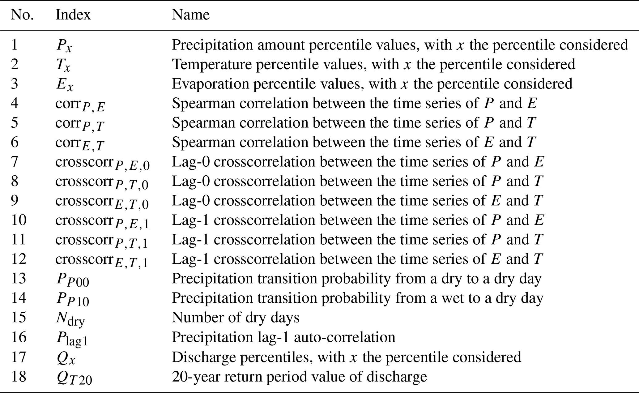
Besides the choice of time frames and data, also the choice of validation indices is of key importance. Maraun and Widmann (2018a) stress that these indices should only be indirectly affected by the bias adjustment, as only validating on adjusted indices can be misleading. Such adjusted indices are the precipitation intensity, temperature and evaporation, which are used to build the transfer function in the historical setting and should be corrected by construction. Under bias stationarity, this correction will be carried over to the future, possibly hiding small inconsistencies that may arise for extreme values. If the bias is not stationary, the effect might be different between adjusted and indirectly affected indices. As such, besides the three adjusted variables (indices 1 to 3 in Table 1) and their correlations (indices 4 to 12, which are directly adjusted by some of the methods), also indices based on the precipitation occurrence and on the discharge Q are used. The occurrence-based indices (13 to 16) allow for assessing how the methods influence the precipitation time series structure. The discharge-based indices (17 and 18) allow for the assessment of the impact of the different bias-adjusting methods on simulated river flow. The discharge-based indices combine the information of the other indices by routing through the rainfall-runoff model. They are the most important aspect of the assessment, as they indicate the natural hazard. As the percentiles focus mostly on the extremes, the Perkins skill score (PSS) (Perkins et al., 2007) is used to assess the adjustment of the full probability density function (PDF) of the variables. All indices are calculated taking all days into account, instead of only calculating them on wet days, as some of the multivariate bias-adjusting methods do not discriminate between wet or dry days in their adjustment.

Table 1 Overview of the indices used.

The indices are all calculated on a seasonal basis for both the calibration and validation period. By comparing over these periods, we can relate the performance to either the method itself or to bias (non)stationarity, on a seasonal basis. The seasons were defined as follows: winter (DJF), spring (MAM), summer (JJA) and autumn (SON).

2.4 Bias nonstationarity

In a study on possible changes in bias, Maurer et al. (2013) proposed the R index:

$$\begin{array}{}\text{(1)}& R=\mathrm{2}{\displaystyle \frac{\mid {\mathrm{bias}}_{\mathrm{f}}-{\mathrm{bias}}_{\mathrm{h}}\mid }{\mid {\mathrm{bias}}_{\mathrm{f}}\mid +\mid {\mathrm{bias}}_{\mathrm{h}}\mid }},\end{array}$$

where bias_f and bias_h are the biases in respectively the future and historical time series, calculated on the basis of the observations and raw climate simulations. The R index takes a value between 0 and 2. If the index is greater than 1, the difference in bias between the two sets is larger than the average bias of the model and it is likely that the bias adjustment would degrade the RCM output rather than improve it. The index is calculated for the indices used for validation in order to have an indication of the influence of bias nonstationarity on these indices. Besides for the indices, the R index is also calculated for the average and standard deviation of each variable, in order to be able to more easily visualize the changes in distribution.

2.5 Hydrological model

Similar to Pham et al. (2018), we use the probability distributed model (PDM, Moore, 2007; Cabus, 2008), a lumped conceptual rainfall-runoff model to calculate the discharge for the Grote Nete watershed in Belgium. This model uses precipitation and evaporation time series as inputs to generate a discharge time series. The PDM as used here was calibrated (RMSE = 0.9 m³ h⁻¹; see Pham et al. (2018) for more details) using the particle swarm optimization algorithm (PSO, Eberhart and Kennedy, 1995). As in Pham et al. (2018), it was assumed that the differences between meteorological conditions in the Grote Nete watershed and Uccle are negligible, and thus the adjusted data for the Uccle grid cell can be used as a forcing for the PDM. This assumption is based on the limited distance of 50 km between the stations used for the observations in Uccle and the gauging station used for the PDM calibration. As mentioned before, the region has a flat topography and, hence, the climatology can be considered to be similar. Furthermore, the goal is not to make predictions, but to assess the impact of different bias adjustment methods on the discharge values. To calculate the bias on the indices, observed, raw and adjusted RCM time series were used as forcing for this model. The discharge time series generated by the observations is considered to be the “observed” discharge, and biases are calculated in comparison with this time series.

2.6 Validation metrics

The residual biases relative to the observations and to the model bias are often used in this paper to graphically present and interpret the results. These residual biases are based on the “added value” concept (Di Luca et al., 2015) and enable a comparison based on two aspects. The first aspect is the extent of the bias removal relative to the original value for the corresponding index for the observation time series, and the second is the performance in removing the bias. The use of the residual biases allows for a detailed study and comparison of the effect of bias adjustment on the different indices.

The residual bias relative to the observations RB_O for an index k is calculated as follows:

$$\begin{array}{}\text{(2)}& {\mathrm{RB}}_{\mathrm{O}}\left(k\right)=\mathrm{1}-{\displaystyle \frac{\mid {\mathrm{bias}}_{\mathrm{raw}\left(k\right)}\mid -\mid {\mathrm{bias}}_{\mathrm{adj}\left(k\right)}\mid }{\mid \mathrm{obs}\left(k\right)\mid }},\end{array}$$

with raw(k) the raw climate model simulations, adj(k) the adjusted climate model simulations and obs(k) the observed values for index k.

The residual bias relative to the model bias RB_MB for an index k is calculated as follows:

$$\begin{array}{}\text{(3)}& {\mathrm{RB}}_{\mathrm{MB}}\left(k\right)=\mathrm{1}-{\displaystyle \frac{\mid {\mathrm{bias}}_{\mathrm{raw}\left(k\right)}\mid -\mid {\mathrm{bias}}_{\mathrm{adj}\left(k\right)}\mid }{\mid {\mathrm{bias}}_{\mathrm{raw}\left(k\right)}\mid }}.\end{array}$$

Absolute values are used in Eqs. (2) and (3) to compute the absolute difference between the raw and adjusted values, thus neglecting a possible change of sign of the bias. If the values of these residual biases are lower than 1 for an index, the method performs better than the raw RCM for this index. The best methods have low scores on both residual biases for as many indices as possible. The low scores imply that the bias adjustment is both effective and has a clear impact relative to the observations. If only RB_MB has a low value (< 0.5), then the bias adjustment was effective, but it had a limited impact relative to the observations. In contrast, if only RB_O has a low value, then the bias adjustment may be limited, but even this limited bias adjustment had an impact relative to the observations.

3 Bias-adjusting methods

3.1 Occurrence-bias adjustment: thresholding

One of the deficiencies of RCMs, especially in northwestern Europe, is the so-called “drizzle days” (Gutowski et al., 2003; Themeßl et al., 2012; Argüeso et al., 2013), during which small amounts of precipitation are simulated while these days should have been dry. This has an influence on the temporal structure of the simulated time series and should thus be adjusted (Ines and Hansen, 2006). This is commonly done in an occurrence-bias-adjusting step before the main step, the intensity-bias adjustment. In this study, we use the thresholding occurrence-bias-adjusting method, which is one of the most common occurrence-bias-adjusting methods (e.g., Hay and Clark, 2003; Schmidli et al., 2006; Ines and Hansen, 2006). This method is only applicable in regions where the assumption holds that the simulated time series has more wet days than the observed time series. This is the case for northwestern Europe (Themeßl et al., 2012) and Belgium in particular. An advanced version of the thresholding method is used here. To adjust the number of wet days, the number of dry days in both the observations and the simulations are calculated. The difference in dry days between the two periods, ΔN, is the number of days of the simulated time series that have to be adapted. If ΔN days have to be converted to dry days, then the ΔN days with the lowest amounts of precipitation are changed to dry days. ΔN is computed for the past and applied in the future and consequently relies on the bias stationarity assumption. However, as thresholding is used prior to all methods, the influence of possible bias nonstationarity on ΔN is assumed to be negligible. Besides, as is shown in Sect. 4.1, the number of dry days is stationary for the time frames studied in this paper.

In this advanced version of thresholding, some considerations are made. First, a day is considered wet if its simulated precipitation amount is above 0.1 mm, to account for measurement errors in the observations. Second, the adjustment is done on a monthly basis, to account for the temporal structure in the observed time series. Third, both historical and future simulations are adjusted, to ensure that the bias can be transferred from the historical to the future time period.

3.2 Univariate intensity-bias-adjusting methods

3.2.1 Quantile delta mapping

The “quantile delta mapping” (QDM) method was first proposed by Li et al. (2010). Its main idea is to preserve the climate simulation trends: it takes trend nonstationarity (changes in the simulated distribution) into account to a certain degree. Although it handles temperature adjustments well, it gives unrealistic values for precipitation and was therefore extended by Wang and Chen (2014) for precipitation adjustment. By combining the methods by Li et al. (2010) (“equidistant CDF-matching”) and Wang and Chen (2014) (“equiratio CDF-matching”), Cannon et al. (2015) developed the QDM method.

Mathematically, this method can be written as

$$\begin{array}{}\text{(4)}& x_i^{\mathrm{fa}}=x_i^{\mathrm{fs}}+F_{x^{\mathrm{ho}}}^{-\mathrm{1}}\left(F_{x^{\mathrm{fs}}}\left(x^{\mathrm{fs}}\right)\right)-F_{x^{\mathrm{hs}}}^{-\mathrm{1}}\left(F_{x^{\mathrm{fs}}}\left(x^{\mathrm{fs}}\right)\right)\end{array}$$

in the additive case and

$$\begin{array}{}\text{(5)}& x_i^{\mathrm{fa}}=x_i^{\mathrm{fs}}{\displaystyle \frac{F_{x^{\mathrm{ho}}}^{-\mathrm{1}}\left(F_{x^{\mathrm{fs}}}\left(x^{\mathrm{fs}}\right)\right)}{F_{x^{\mathrm{hs}}}^{-\mathrm{1}}\left(F_{x^{\mathrm{fs}}}\left(x^{\mathrm{fs}}\right)\right)}}\end{array}$$

in the ratio or multiplicative case. The superscripts hs, ho, fs and fa indicate respectively the historical simulations, the historical observations, the future simulations and the adjusted future. In this paper, the additive version is used for temperature time series and the multiplicative one for precipitation and evaporation time series. This choice is based on the work of Wang and Chen (2014), who have shown that using the additive adjustment for precipitation results in unrealistic precipitation values and introduced a multiplicative adjustment. For evaporation, we follow the few available studies (e.g., Lenderink et al., 2007) in using the same adjustment as for precipitation.

For computational ease, an empirical CDF was used in the QDM equations (as in Gudmundsson et al., 2012; Gutjahr and Heinemann, 2013 for other quantile mapping methods). It is also important to note that for precipitation, Eq. (5) was applied only on the days considered wet, i.e., with a precipitation higher than 0.1 mm. For consistency, a threshold of 0.1 mm was also used for evaporation. It is important to note that although QDM is only applied on wet days, it can still transform low-precipitation wet days into days that are considered to be dry (e.g., with a precipitation amount < 0.1 mm) if the ratio in Eq. (5) is small enough.

3.2.2 Modified quantile delta mapping

Pham (2016) proposed another version of QDM, following the delta change philosophy (Olsson et al., 2009; Willems and Vrac, 2011): the trend established by the RCM is assumed to be more thrust-worthy than the absolute value itself. When applying this type of methods, the simulated change between the historical and the future is applied to the observations. Thus, instead of the future simulations, the historical observations are adjusted to the future “observations”. As Johnson and Sharma (2011) mention, this workflow could be problematic for future impact assessment, as it inherits the temporal structure of the historical observations. This method is mathematically very similar to the QDM method, exchanging the roles of x^fs and x^ho. Thus, it is named “modified quantile delta mapping” (mQDM) and can for the additive case be written as

$$\begin{array}{}\text{(6)}& x_i^{\mathrm{fa}}=x_i^{\mathrm{ho}}+F_{x^{\mathrm{fs}}}^{-\mathrm{1}}\left(F_{x^{\mathrm{ho}}}\left(x^{\mathrm{ho}}\right)\right)-F_{x^{\mathrm{hs}}}^{-\mathrm{1}}\left(F_{x^{\mathrm{ho}}}\left(x^{\mathrm{ho}}\right)\right).\end{array}$$

The ratio version is given by

$$\begin{array}{}\text{(7)}& x_i^{\mathrm{fa}}=x_i^{\mathrm{ho}}{\displaystyle \frac{F_{x^{\mathrm{fs}}}^{-\mathrm{1}}\left(F_{x^{\mathrm{ho}}}\left(x^{\mathrm{ho}}\right)\right)}{F_{x^{\mathrm{hs}}}^{-\mathrm{1}}\left(F_{x^{\mathrm{ho}}}\left(x^{\mathrm{ho}}\right)\right)}}.\end{array}$$

For the implementation, the same principles were used as for the QDM method: empirical CDFs and a minimum value of 0.1 mm d⁻¹ to be considered a wet day.

3.3 Multivariate intensity-bias-adjusting methods

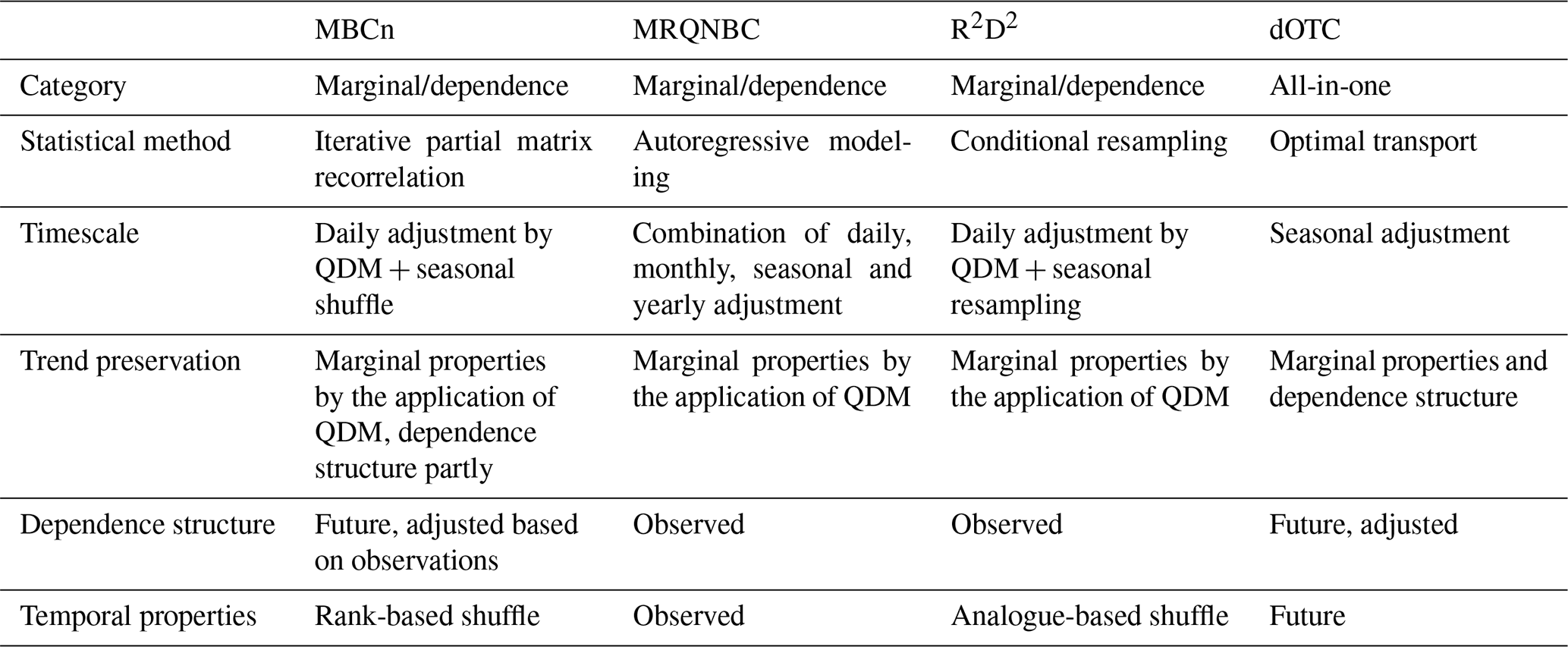
The increasing number of multivariate bias-adjusting methods throughout the 2010s urges the need to classify them according to their properties. One possible classification was done by Vrac (2018), who proposed the “marginal/dependence” versus the “successive conditional” approach. The former approach separately adjusts the 1D-marginal distributions and the dependence structure and is applied in, e.g., Vrac and Friederichs (2015), Cannon (2018) and Vrac (2018). These two components are then recombined to obtain data that are close to the observations for both marginal and multivariate aspects. The latter approach consists of adjusting a variable conditionally on the variables already adjusted. This procedure is applied successively to each variable. Examples can be found in, e.g., Piani and Haerter (2012), Li et al. (2014) and Dekens et al. (2017). Vrac (2018) discusses the limitations of the “successive conditional” approach and advocates for the use of the more robust and coherent “marginal/dependence” approach. Hence, “successive conditional” methods are not included in the present paper. Robin et al. (2019) and François et al. (2020) extended the classification by introducing the “all-in-one” approach, which adjusts the marginal variables and the correlations simultaneously, “dynamical optimal transport correction” (dOTC, Robin et al., 2019) being such a method.

Another perspective on the multivariate bias-adjusting methods is to consider the amount of temporal adjustment that is allowed or applied by the method. This is important, as the amount of temporal adjustment is intrinsically linked with the main goal, the adjustment of the multivariate distribution of the variables. This distribution, in which the dependence is characterized by the underlying copula (Nelsen, 2006; Schölzel and Friederichs, 2008), can be estimated using the ranks. Thus, to adjust the multivariate distribution, the ranks of the climate model are replaced by those of the observations, using methods such as the “Schaake shuffle” (Clark et al., 2004; Vrac and Friederichs, 2015). This implies that the temporal structure and trends of the climate model will be altered, which may have a considerable impact (François et al., 2020). This impact is especially large when multiday characteristics strongly matter, such as in applications as the hydrological example we use in this study (Addor and Seibert, 2014). Vrac (2018) mentions this necessity to modify the temporal structure and rank chronology of the simulations. Yet, he also mentions that the extent of this modification is still a matter of debate. Cannon (2016) describes this as the “knobs” that control whether marginal distributions, inter-variable or spatial dependence structure and temporal structure are more informed by the climate model or the observations. Thus, the choice between the temporal structure of the climate model and unbiased dependence structures is a trade-off that has to be made. Some methods, such as those by Vrac and Friederichs (2015), Mehrotra and Sharma (2016) and Nguyen et al. (2018), rely on the observations for their temporal properties, while other methods try to find the middle ground (e.g., Vrac, 2018 and Cannon, 2018). A last perspective, which is not limited to multivariate methods, is that of trend preservation, i.e., the capacity of methods to preserve the changes simulated by the climate model, such as changes in mean, extremes and temporal structure. Although the amount of trend preservation or adjustment has been a matter of debate (Ivanov et al., 2018), Maraun (2016) argues that it is sensible to preserve the simulated changes and hence the climate change signal, if the model simulation is credible. As such, trend preservation interacts with bias nonstationarity: non-stationarity can be seen as the divergence between the observed and simulated trends. Hence, in a nonstationary context, trend-preserving methods may be disadvantaged, as they will assume that the simulated trend is trustworthy. In the univariate setting, QDM is an example of a trend-preserving method.

Our choice of multivariate bias-adjusting methods takes the above classification into account. The oldest method in the comparison is “multivariate recursive quantile nesting bias correction” (MRQNBC) (Mehrotra and Sharma, 2016). This method replaces the simulated correlations by those of the observations and is a “marginal/dependence” method according to François et al. (2020). As QDM is used for the marginal distributions, the latter are preserved. However, MRQNBC does not preserve the changes in dependence. “Multivariate bias correction in n dimensions” (Cannon, 2018) is both a “marginal/dependence” method and a method that tries to combine information from the climate model and the observations. Similar to MRQNBC, it explicitly preserves the simulated changes in the marginal distributions by applying QDM for the marginal distributions. As the simulated dependence structure is the basis for the adjustment, it will be slightly preserved. The “rank resampling for distributions and dependences” (R²D², Vrac, 2018; Vrac and Thao, 2020b) method preserves the rank correlation of the observations, but it allows the climate model to have some influence on the temporal properties. It is also a “marginal/dependence” method: in the present paper, QDM is used as its univariate routine and thus the changes in marginal distributions are preserved by R²D². The last method, “dynamical optimal transport correction” (Robin et al., 2019), differs considerably from the other two methods: it generalizes the “transfer function” principle using the “optimal transport” paradigm (Villani, 2008), thereby defining a new category of multivariate bias-adjusting methods: the above-mentioned all-in-one approach. It is the only method that explicitly preserves the simulated changes in both the marginal distributions and the dependence structure. Although far from complete, by comparing these four methods, a broad view of the different approaches in multivariate bias adjustment can be obtained. The main principles of the bias-adjusting methods are summarized in Table 2.

Table 2 Overview of the multivariate bias-adjusting methods.

3.3.1 Multivariate recursive quantile nesting bias correction

In 2016, Mehrotra and Sharma (2016) proposed a new multivariate bias adjustment method, named “multivariate recursive quantile nesting bias correction” (MRQNBC), based on a combination of several older methods by Johnson and Sharma (2012), Mehrotra and Sharma (2012) and Mehrotra and Sharma (2015) and by incorporating QDM as the univariate routine for adjusting the marginals. The underlying idea of this method is to adjust on more than one timescale and to nest the results of the different timescales within each other. The adjustment on multiple timescales is rarely incorporated in bias-adjusting methods (Haerter et al., 2011). On each timescale, the biases in lag-0 and lag-1 autocorrelation and lag-0 and lag-1 cross-correlation coefficients, i.e., the persistence attributes, are adjusted, instead of focusing on the mean or the distribution. The biases are adjusted by replacing the modeled persistence attributes with observed persistence attributes, on the basis of autoregressive expressions. Besides replacing the simulated temporal properties with the observed ones, this implies that the simulated dependence structure is also replaced with the observed structure. As QDM is applied on each timescale, the marginal properties are preserved.

After adjusting all timescales, the final daily result is calculated by weighing all timescales. However, as the nesting method cannot fully remove biases at all timescales, Mehrotra and Sharma (2016) suggested to repeat the entire procedure multiple times. Yet, in our case multiple repetitions exacerbated the results. Non-realistic outliers created by the first repetition influenced the subsequent repetitions, creating even more non-realistic values. This was most clearly seen for precipitation. As a bounded variable, precipitation is most sensitive for non-realistic values. Nonetheless, running the method just once yielded satisfactory results for most variables. A full mathematical description of the method can be found in Mehrotra and Sharma (2016).

3.3.2 Multivariate bias correction in n dimensions

In 2018, Cannon (2018) proposed the “multivariate bias correction in n dimensions” (MBCn) method as a flexible multivariate bias-adjusting method. The method's flexibility has attracted some attention, and it has already been used in multiple studies (Räty et al., 2018; Zscheischler et al., 2019; Meyer et al., 2019; François et al., 2020). This method consists of three steps. First, the multivariate data are rotated using a randomly generated orthogonal rotation matrix, adjusted with the additive form of QDM, and rotated back until the calibration period model simulations converge to the observations. This convergence is verified on the basis of the energy distance (Rizzo and Székely, 2016). Second, the validation period simulations are adjusted using QDM, as this method preserves the simulated trends. As the last step, these adjusted time series are shuffled using the Schaake shuffle (Clark et al., 2004) based on the rank order of the rotated data set. This shuffle can remove temporal structure in the resulting time series. A full mathematical description of the method can be found in Cannon (2018).

3.3.3 Rank resampling for distributions and dependences

One of the most recent methods studied in this paper is the “rank resampling for distributions and dependences” (R²D²) method, which was designed by Vrac (2018) as an improvement of the older EC–BC method (Vrac and Friederichs, 2015). Recently, R²D² was further extended for better multisite and temporal representation by Vrac and Thao (2020b) (R²D² v2.0). This method is a marginal/dependence multivariate bias-adjusting method, which adjusts the simulated climate dependence by resampling from the observed dependence. The resampling is applied through the search for an analogue for the ranks of a simulated reference dimension in the observed time series, which makes this an application of the analogue principle (Lorenz, 1969; Zorita and Von Storch, 1999) in bias adjustment. A detailed mathematical description can be found in Vrac (2018) and Vrac and Thao (2020b).

In the present application of R²D², QDM was used as the univariate bias-adjusting method to ensure consistency with the other multivariate bias-adjusting methods. This ensures the preservation of the changes in the marginal distribution. Each variable (precipitation, evaporation and temperature) was in turn used as the reference dimension. As the present study was limited to a single grid cell, the use of additional data was limited. However, to ensure that the selection of analogues is diverse enough, five lags were used to search for analogues, three of which were retained in the resampling. Finally, the results for the three variables were averaged to present the final R²D² result.

3.3.4 Dynamical optimal transport correction

Recently, Robin et al. (2019) indicated that the notion of a transfer function in quantile mapping can be generalized to the theory of optimal transport. Optimal transport is a way to measure the dissimilarity between two probability distributions and to use this as a means for transforming the distributions in the most optimal way (Villani, 2008; Peyré and Cuturi, 2019).

Optimal transport was used by Robin et al. (2019) to adjust the bias of a multivariate data set in the “dynamical optimal transport correction” method (dOTC), which extends the “CDF-transform” (CDF-t) bias-adjusting method (Michelangeli et al., 2009) to the multivariate case. dOTC calculates the optimal transport plans from X^ho to X^hs (the bias between the model and the simulations) and from X^hs to X^fs (the evolution of the model). The combination of both optimal transport plans allows for bias adjustment while preserving the simulated changes in both marginal properties and the dependence structure. A full mathematical description of the method can be found in Robin et al. (2019).

3.4 Experimental design

Prior to all intensity-bias-adjusting methods, the thresholding occurrence-adjusting method was applied. In the intensity-bias-adjustment step, a balance was sought between randomness and computational power for the calculation of the intensity-bias-adjusting methods. Methods with randomized steps were repeated. As such, 10 calculations were made for dOTC. The bias-adjustment methods were always applied with seasonal input to ensure consistency among all methods. Only for MRQNBC, seasonal input was not considered, as this method has a seasonal component. As MRQNBC is developed to take multiple timescales into account, the comparison with the other multivariate bias-adjusting methods allows one to discern whether fine-tuning for seasons or a more general timescale-focused method is the best approach to deal with seasonally varying biases.

The resulting values of each index were averaged for further comparison. Biases on the indices were always calculated as raw or adjusted simulations minus observations, indicating a positive bias if the raw or adjusted simulations are larger than the observations and a negative bias if the simulations are smaller.

4 Results

In this section, we will first discuss the R index calculations for bias change. Next, we will discuss the validation indices. For the validation indices, first the indices based on the adjusted variables are discussed, followed by an elaboration on the indices based on the derived variables. As the effect on discharge is the overarching goal of this paper and the discharge indices are affected by all other indices, those will be discussed last.

4.1 Bias change

The results for the R index vary considerably depending on the season: bias nonstationarity (R index values > 1) is present for all variables, but the extent varies (Tables 3 and 4). For precipitation (Table 3), bias nonstationarity is most clear in winter and summer for the highest percentiles (P₉₉ and P_99.5). For temperature, winter, spring and summer all show some high R index values, but while winter has high R index values for all percentiles, the nonstationarity is restricted to the lower to middle percentiles (T₅, T₂₅, T₅₀ and T₇₅) for spring and the lower percentiles (T₅ and T₂₅) for summer. This is reflected in the mean and standard deviation: both are nonstationary for winter, whereas only the mean is nonstationary for spring and neither the mean nor the standard deviation is nonstationary for summer. In autumn, the behavior is less clear: two percentiles (P₅₀ and P₉₅) have an R index value of 2, but unlike the other seasons, there is no apparent pattern as these values are far apart. However, the standard deviation has an R index value higher than 1 for autumn temperatures, indicating that some bias nonstationarity could be present. For evaporation, spring has the clearest bias nonstationarity: almost all percentiles have an R index value higher than 1. For the other seasons, the nonstationarity is less striking, although present. For winter and autumn, E₇₅ has an R index value of 1 or higher and a clearly nonstationary standard deviation, while in summer, E₂₅ and E₅₀ have an R index value higher than 1, although neither mean nor standard deviation is clearly nonstationary.

Table 3 R index values for the variables for 1970–1989 as historical period and 1998–2017 as future period.

Table 4 R index values for occurrence and correlation for 1970–1989 as historical period and 1998–2017 as future period.

Table 4 presents the R index values for occurrence and correlation. For occurrence, the bias nonstationarity seems limited: only in spring and autumn, the R index value for precipitation lag-1 autocorrelation is higher than 1. For correlation, the bias nonstationarity is also limited, although some of the correlations of evaporation and either temperature or precipitation have an R index value higher than 1, but this depends on the season (crosscorr${}_{E,T,\mathrm{0}}$ and crosscorr${}_{E,T,\mathrm{1}}$ in spring, crosscorr${}_{E,T,\mathrm{1}}$ in winter, corr_E,T in summer and corr_P,E in autumn).

Many of the R index values thus indicate that the bias changes between the two periods considered here (1970–1989 versus 1998–2017) might already be large enough to have an effect on the bias adjustment. As these periods are only separated by 10 years, this is an important indicator for the bias adjustment of late 21st century data, just as Chen et al. (2015) mentioned. The results vary substantially among seasons, variables and distributions of the variables. Although this could give an indication of the reason for poor performance for some of these indices, it is impossible to state exactly what causes the bias nonstationarities purely based on these results. Possible causes could be that recent trends such as those in precipitation extremes (Papalexiou and Montanari, 2019) are poorly captured by the models and that limiting mechanisms such as soil moisture depletion (Bellprat et al., 2013) are poorly modeled or that natural variability (Addor and Fischer, 2015) influences the biases. However, discussing this in depth is out of the scope of the present study and deserves a separate study. In what follows, we will focus on the performance of the bias-adjusting methods and whether or not there is a link with these nonstationarities.

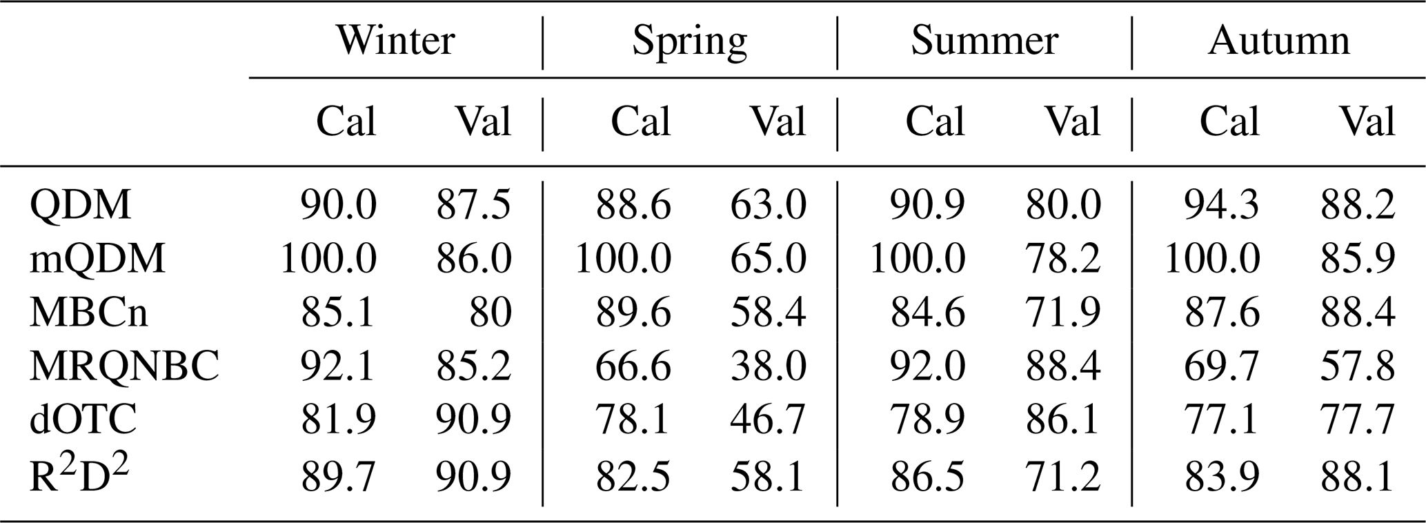
4.2 Precipitation amount

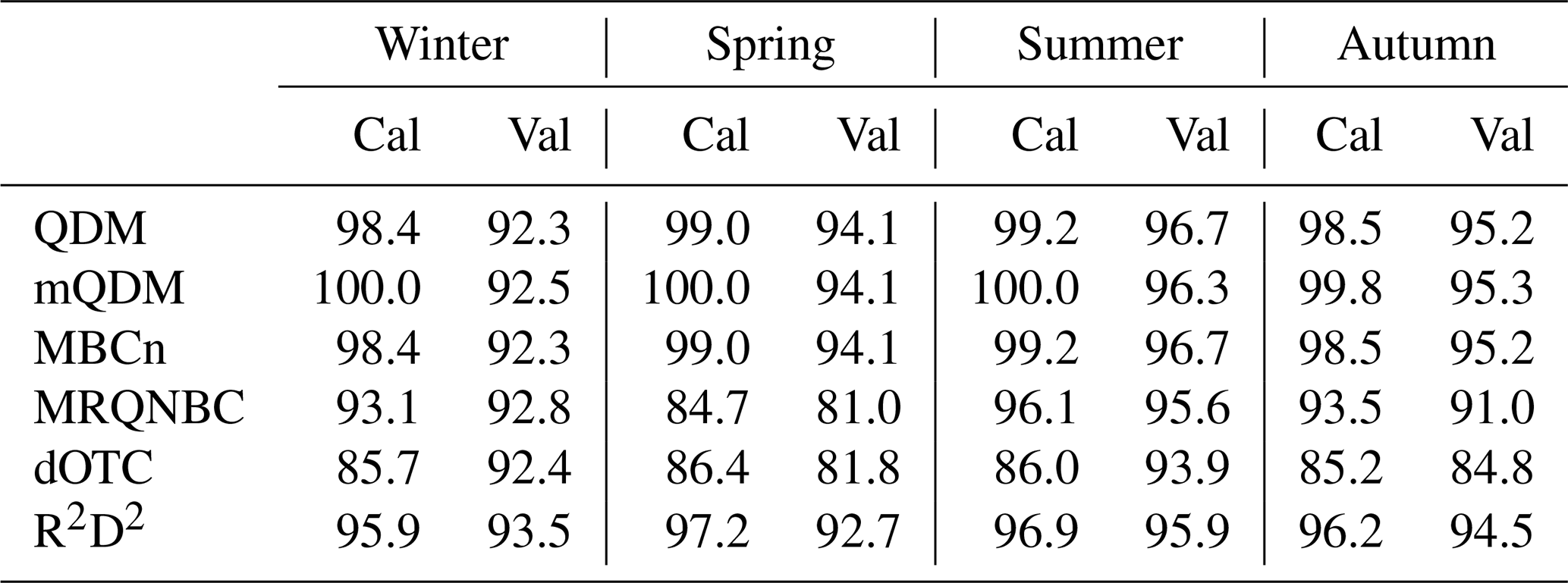
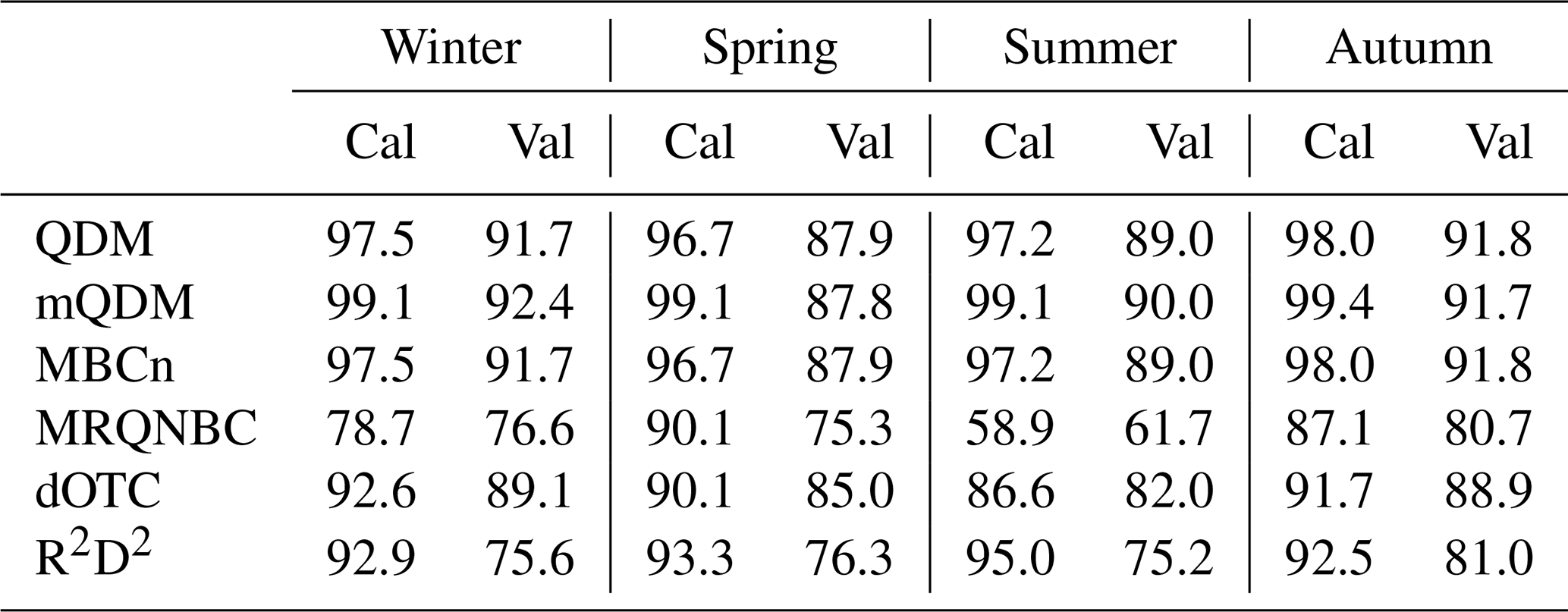
The Perkins skill score (PSS) for precipitation (Table 5) indicates that the PDFs of the observations and adjusted simulations agree rather well. These scores are similar in the calibration and validation period. Nonetheless, some aspects deserve more attention. By focusing on the calibration period, it is possible to understand the basic performance of the methods. By construction, mQDM has a PSS of 100 %. A more peculiar aspect is the slightly lower PSS of MRQNBC and the clearly lower PSS of dOTC: this indicates that these methods are harder to calibrate correctly and thus that the results might be influenced by a poor calibration. Lastly, the results for QDM and MBCn are the same. This corresponds to the expectation, as the marginal aspects of both methods are the same by construction. Moving on to the validation period, it is clear that all methods generally perform worse than in the calibration period. This has been reported before (e.g., Guo et al., 2020). Based on the PSS values alone, it is impossible to distinguish the cause of this decrease in performance. Note that the performance of dOTC increases or is rather stable, making it more difficult to discuss this method.

Table 5 PSS values for precipitation in the calibration (Cal) and validation (Val) periods (%).

The relatively good performance for the full PDF contrasts with the bias adjustment of the extreme values. Figures 1 and 2 present the RB_O and RB_MB values for the highest P percentiles. The lowest percentiles are not included in these plots, as their RB_O or RB_MB values are for most methods lower than 0. In the calibration period (Fig. 1), all methods perform relatively well. For QDM, mQDM and MBCn, the adjustment is nearly perfect (as also indicated by the PSS values), but even for dOTC, the adjustment is acceptable, with the RB_O and RB_MB values for many indices lower than 1. The contrast with the validation period (Fig. 2) can be easily seen for QDM, mQDM and MBCn. Closer inspection yields more details on differences among seasons. For winter (blue) and summer (yellow), only P₇₅ and P₉₀ can be plotted in the validation period, whereas for spring and autumn all percentiles from P₇₅ to P_99.5 can be plotted for all methods. In winter and summer, the highest percentiles have RB_O or RB_MB values higher than 1. To enable comparison between calibration and validation period and between different variables, all plots were chosen to have the same ranges; hence the residual biases for these poorly adjusted variables cannot be plotted. The poor adjustment of the high percentiles in winter and summer is probably caused by bias nonstationarity: the R index values for these percentiles are higher than 1, in contrast with the low and well-adjusted higher percentiles for spring and autumn precipitation. However, although P₉₅ has an R index value lower than 1 for both winter and summer, it is also poorly adjusted. This illustrates that the R index gives an indication of the nonstationarity, but it also hides information on the size of the biases. For summer, the bias for P₉₅ changes from 5.09 mm in the calibration period to 1.89 mm in the validation period, a change of over 3 mm. For winter, the bias changes from 1.44 mm in the calibration period to 0.52 mm in the validation period, a change of almost 1 mm. Yet, these differences have a very similar R index value.

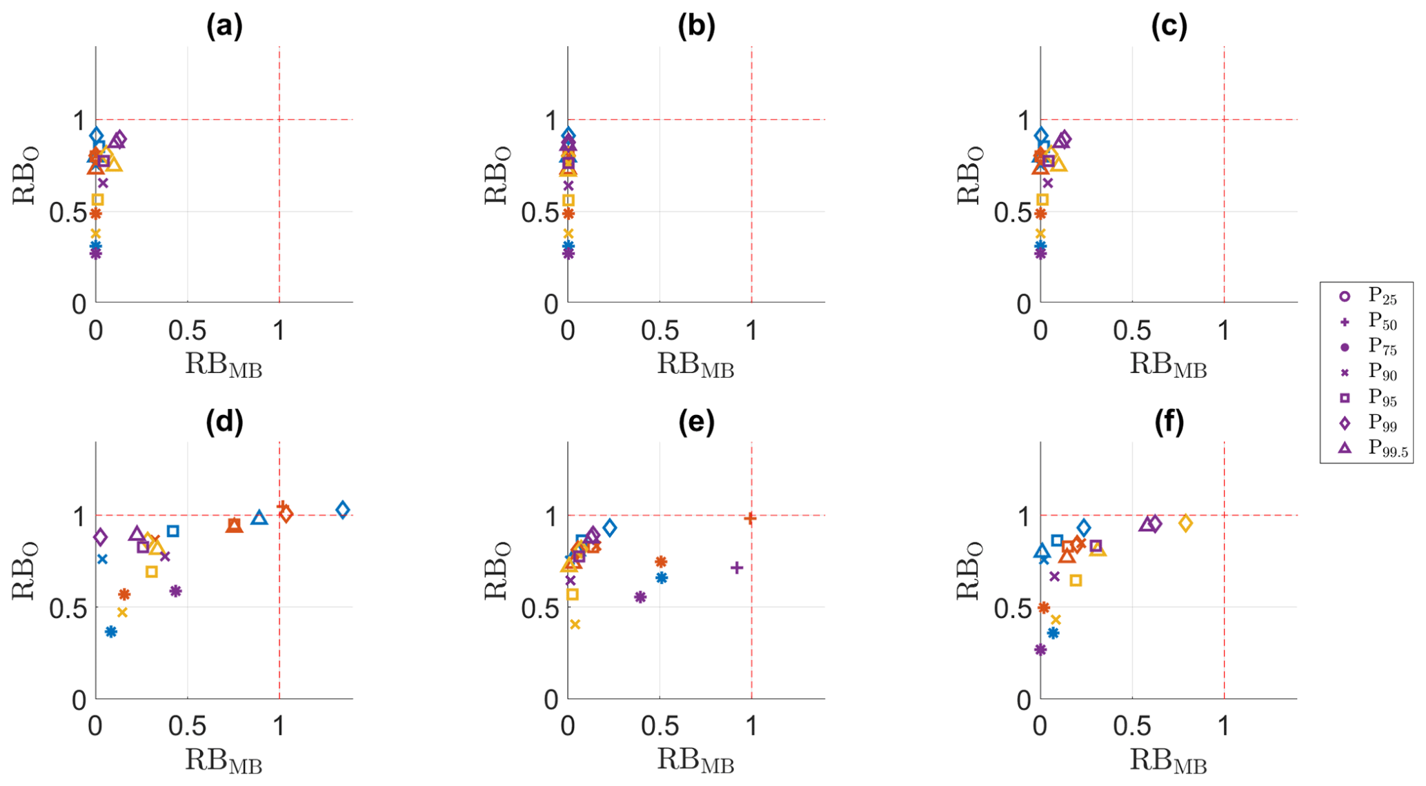
Figure 1 RB_MB versus RB₀ for the precipitation indices in the calibration period. (a) QDM, (b) mQDM, (c) MBCn, (d) MRQNBC, (e) dOTC, (f) R²D². Winter: blue, spring: ochre, summer: yellow, autumn: purple.

Figure 2 RB_MB versus RB₀ for the precipitation in the validation period. (a) QDM, (b) mQDM, (c) MBCn, (d) MRQNBC, (e) dOTC, (f) R²D². Winter: blue, spring: ochre, summer: yellow, autumn: purple.

The nonstationarity seen in Figs. 1 and 2 is not apparent from the PSS, as it only occurs in the tail of the distribution. This also follows from the R index values for the mean and standard deviation in winter and summer. Only for standard deviation, the R index value indicates nonstationarity in winter and summer: the values are respectively 1.79 and 1.56. Thus, the nonstationarity of the extremes and the standard deviation seem to be linked.

The methods seem to perform rather similarly within every season. Although the RB_MB values vary, indicating that for some methods the bias is removed to a larger extent, the RB_O values are similar, indicating that relative to the observations, the influence of the difference in removed bias is low. The similarity in RB_O values is related to the observed values, which increase more than the biases with increasing percentiles. Hence, the RB_O values are often higher for higher percentiles. Although the methods perform similarly on a seasonal basis, small differences may accumulate on a yearly basis. For example, on a yearly basis, the mean number of heavy precipitation days (R10, one of the ETCCDI indices Zhang et al., 2011) is well presented by all adjusted simulations (Fig. 3), but the yearly variance clearly depends on the method: MRQNBC overestimates the variance, whereas the other methods slightly underestimate it.

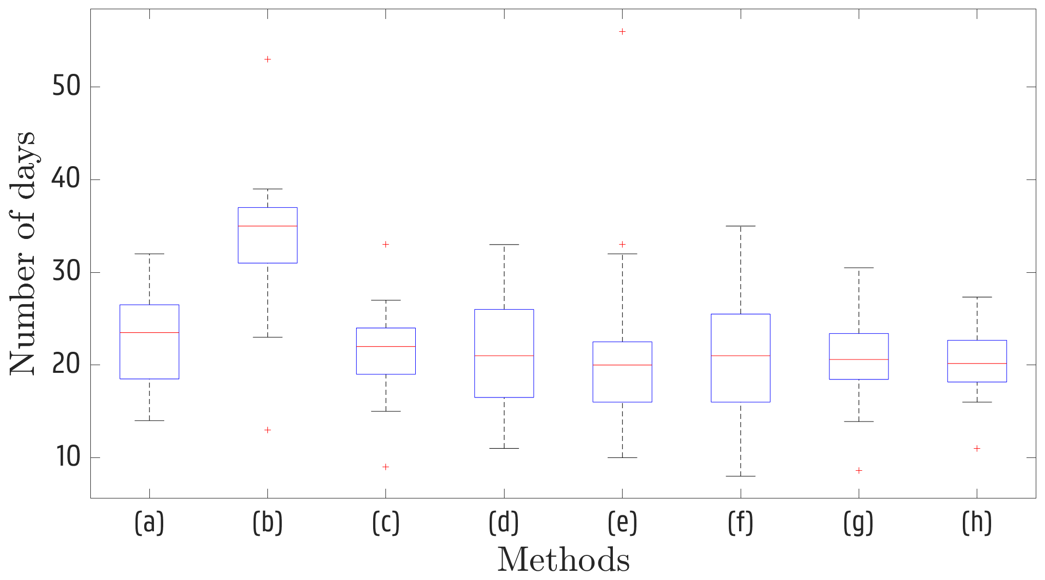
Figure 3 Box plot of the annual number of days with precipitation higher than 10 mm (ETCCDI “heavy precipitation” days; see Zhang et al., 2011) in the validation period. (a) Observations, (b) raw simulations, (c) QDM, (d) mQDM, (e) MBCn, (f) MRQNBC, (g)  dOTC, (h) R²D².

For precipitation, bias nonstationarity was present for the highest percentiles in both winter and summer (P₉₉ and P_99.5), with R index values ≥2, the highest possible value. For these percentiles, the adjustment was clearly poorer in the validation period than in the calibration period, indicating that bias nonstationarity has an impact on bias adjustment. This implies that it is important to study the propagation of bias nonstationarity towards discharge assessment. This propagation will be further studied in Sect. 4.7, but a first overview based on literature can already be given. Although a high precipitation depth is not the main driver of floods in northwestern Europe (Berghuijs et al., 2019), it can act as a trigger, especially under climate change and for urban catchments (Sharma et al., 2018). For the latter, the nonstationarity and poor adjustment in summer might be especially relevant, as convective storms can easily cause pluvial floods. However, the hydrological model applied in this study (i.e., PDM) is not meant to model this type of floods. The impact on discharge might thus be more pronounced in winter.

4.3 Temperature

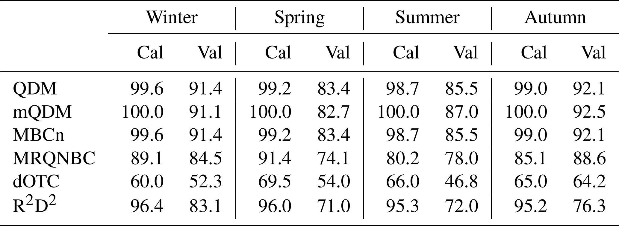
Table 6 displays the PSS values for temperature. In general, the same conclusions can be drawn as for precipitation (Table 5): QDM, mQDM and MBCn perform best in both the calibration and the validation period, with R²D² performing only slightly worse and all methods performing worse in the calibration period. However, for temperature, dOTC performs relatively well, and MRQNBC performs worst for all seasons. Additionally, R²D² shows the sharpest decrease in performance throughout all seasons from the calibration period to the validation period. This decrease is probably caused by the analogue resampling, which does not fully reproduce the original marginal distribution, although it should approximate it.

Table 6 PSS values for temperature in the calibration (Cal) and validation (Val) periods (%).

Although the PDF of the adjusted simulations matches the observed PDF relatively well, a comparison between the RB_MB and RB_O values of the calibration (Fig. 4) and validation period (Fig. 5) shows some clear differences between the seasonal bias adjustment. In the validation period, all methods perform poorly for winter (blue), whereas for the other seasons, at least some methods are able to adjust the raw simulations. For winter, the R index values are high for all percentiles, which indicates that nonstationarity is the probable cause for the poor performance. This is especially clear for QDM, mQDM and MBCn (upper half of the figures). The performance of MRQNBC, dOTC and R²D² (lower half of the figures) is poor in the calibration period as well. In the calibration period, some percentiles have a larger bias after the adjustment for these three methods. This cannot be observed for QDM, mQDM and MBCn, which illustrates that even a relatively small difference in PSS value (92.9 for R²D² versus 97.5 for MBCn) can imply a poorer bias adjustment. Nonetheless, even for these methods there is a clear difference in visible winter markers, indicating a loss of performance from calibration to validation period.

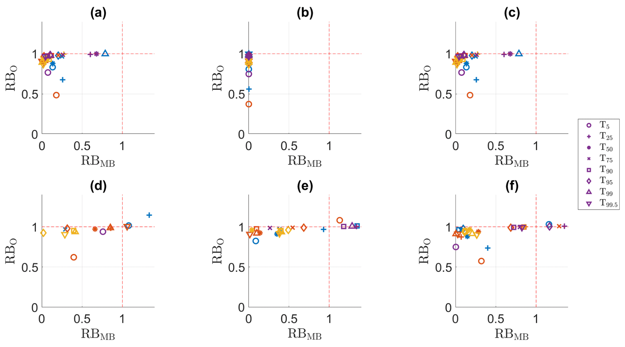
Figure 4 RB_MB versus RB₀ for the temperature indices in the calibration period. (a) QDM, (b) mQDM, (c) MBCn, (d) MRQNBC, (e) dOTC, (f) R²D². Winter: blue, spring: ochre, summer: yellow, autumn: purple.

Figure 5 RB_MB versus RB₀ for the temperature indices in the validation period. (a) QDM, (b) mQDM, (c) MBCn, (d) MRQNBC, (e) dOTC, (f) R²D². Winter: blue, spring: ochre, summer: yellow, autumn: purple.

For spring (ochre), the performance also decreases from calibration to validation period, although not as extensively as for winter. For spring, T₅, T₂₅, T₅₀ and T₇₅ all have larger biases after adjustment than before adjustment. In contrast, in the calibration period, T₅ in spring stands out as best adjusted percentile for all methods (except dOTC; see panel e). The poor performance for these lower T percentiles corresponds to the high R index value (i.e., 2) for all of these percentiles for spring. For summer, this is also observed, although to a smaller extent: only T₅ (with R index value 2) seems to be affected. For autumn, the performance is generally worse in the validation period than in the calibration period, with some percentiles having a larger bias after adjustment. However, because of the limited nonstationarity, conclusions are harder to draw. Nonetheless, it seems that the percentiles with a high R index have the worst performance. As an example, the RB_MB for T₉₅ (R index 2) is higher than 3 for all methods.

All temperature percentiles in winter and the lowest temperature percentiles in spring and summer all have high R index values (an R index of 2 for most of these percentiles) and are poorly adjusted in the validation period. This implies that the lower temperature values are more susceptible to nonstationarity, which should certainly be accounted for when estimating extremes such as cold spells. However, the impact on discharge is expected to be limited. A possible impact of temperature bias nonstationarity could be seen through the generally high rank correlation with evaporation. As the rank correlation is important in the multivariate methods, the bias in temperature could thus propagate to discharge. However, the bias nonstationarity and its impact is mostly present for lower temperature percentiles, which are correlated with lower evaporation percentiles. As such, the poor adjustment of temperature biases seen here will probably have a limited impact on the discharge.

4.4 Potential evaporation

The PSS values for potential evaporation (Table 7) are similar to those for temperature (Table 6) and precipitation (Table 5): QDM, mQDM, MBCn and R²D² all perform very well, but they perform worse in the validation period than in the calibration period. However, in contrast with precipitation and especially temperature, dOTC performs poorly in the calibration period. Given the poor performance in the calibration period, the results for the validation period for dOTC are less interpretable than those for other variables. MRQNBC is in between dOTC and the other methods, with the PSS values depending heavily on the season. For spring and summer, the change between the calibration and validation period is larger than changes for precipitation or temperature, at least for the four well-performing methods. As an example, for spring, the PSS value changes for QDM from 99.2 to 83.4, while for summer this change is from 98.7 to 85.5. Whereas the R index values for spring evaporation are generally high, with only a few below 1, those for summer are less extreme.

Table 7 PSS values for evaporation in the calibration (Cal) and validation (Val) periods (%).

The RB_MB and RB_O results for potential evaporation in the validation period are displayed in Figs. 6 and 7. We will focus here on QDM, mQDM, MBCn and R²D², as the PSS results for the calibration period indicate a generally poorer performance for MRQNBC and dOTC. For every season, all methods perform rather poorly in the validation period and worse than in the calibration period, with QDM, mQDM, MBCN and R²D² performing similarly. Based on the R index values and Table 7, it would seem that spring is most influenced by bias nonstationarity, as many percentiles have an R index value higher than 1 and the PSS values differ considerably for spring. Figure 7 shows that only E₅ (for QDM, mQDM, MBCn, MRQNBC and R²D², respectively panels a, b, d and f), E₉₉ (for QDM, mQDM, MBCn and R²D², respectively panels a, b and f) and E_99.5 (for QDM, mQDM and MBCn, panels a, b and c) have RB_MB and RB_O values lower than 1. Except for E_99.5, this corresponds to the percentiles that have an R index value lower than 1. However, the RB_MB and RB_O values for E_99.5 are close to 1 for the three methods mentioned here. The performance of the bias adjustment methods for this percentile can thus not considered to be good, but at the least it is not worse than the raw climate simulations.

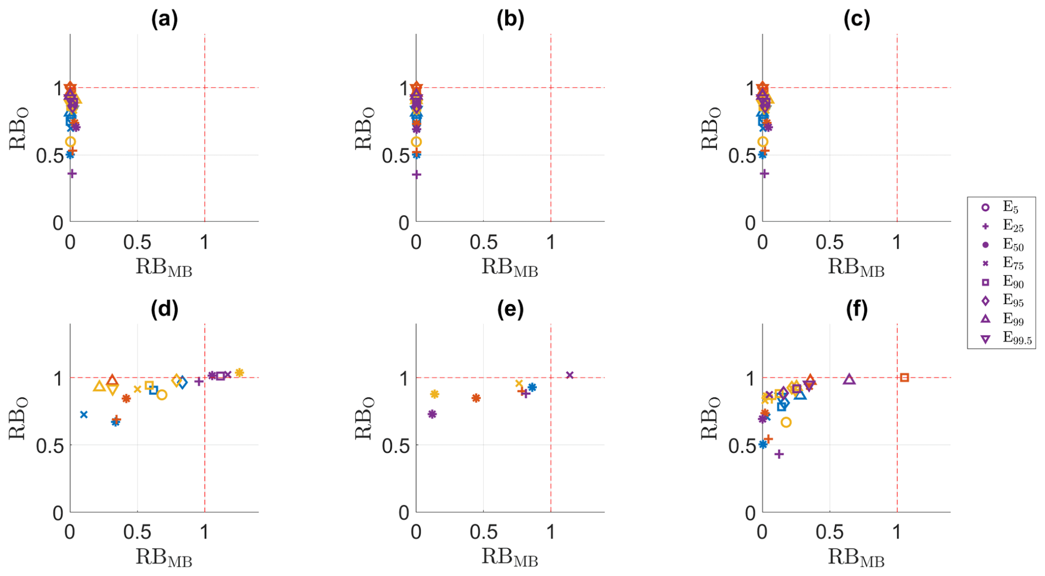
Figure 6 RB_MB versus RB₀ for the potential evaporation indices in the calibration period. (a) QDM, (b) mQDM, (c)  MBCn, (d) MRQNBC, (e) dOTC, (f) R²D². Winter: blue, spring: ochre, summer: yellow, autumn: purple.

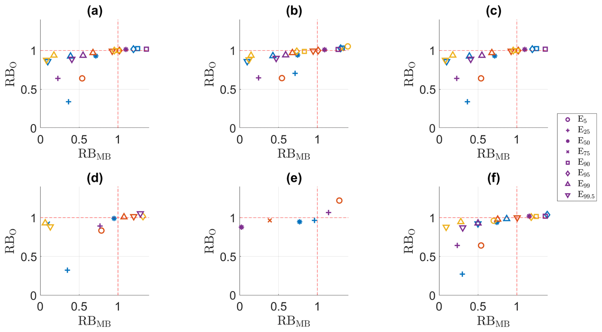
Figure 7 RB_MB versus RB₀ for the potential evaporation indices in the validation period. (a) QDM, (b) mQDM, (c)  MBCn, (d) MRQNBC, (e) dOTC, (f) R²D². Winter: blue, spring: ochre, summer: yellow, autumn: purple.

For the other seasons some differences between the calibration and validation period are worth discussing as well. In winter (blue), where nonstationarity mostly affected the standard deviation, the performance of all methods for all indices is slightly worse in comparison with the calibration period. Only the lower percentiles (E₅ and E₂₅) can be adjusted well by almost every method, although this cannot be seen in the plot for E₅ as this percentile corresponds with a potential evaporation of 0 mm in winter. In summer (yellow), where the R index values indicated some nonstationarity for the lower E percentiles, the performance is poorer in the validation period for most percentiles, with only E₉₉ and E_99.5 clearly performing well for all methods (except dOTC). In autumn (purple), the R index values indicated the largest impact on the standard deviation. As in winter, the best performance is obtained for the lowest percentiles and for the highest percentiles (E₉₉ and E_99.5).

For evaporation, bias nonstationarity was most obvious in spring, with many percentiles having an R index value higher than 1 or even 2. This seemed to have an impact on the bias adjustment, as these percentiles were poorly adjusted in the validation period. For other seasons, there was less nonstationarity; nevertheless, a small impact could be found. However, the results for potential evaporation have to be considered in comparison to the effective bias values for the original simulations and the adjusted simulations: the original biases were relatively small (not shown). This is reflected by the RB_O values. These are high, which indicates that the bias adjustment is limited relative to the observations. Nonetheless, the bias and failure to adjust it could have an impact on discharge. Evaporation is an input for the hydrological model used in this paper and has an influence on soil moisture storage representation. As soil moisture is a major driver for floods in northwestern Europe (Berghuijs et al., 2019), it is important to understand how evaporation biases propagate to the impact model. Yet, the impact of soil moisture is most important in winter, and thus the propagation of evaporation nonstationarity in spring might be limited.

4.5 Correlation

For correlation (Fig. 8), all methods perform relatively well in the validation period. The univariate methods will adopt the dependence structure of either the raw simulations (QDM) or the observations (mQDM), whereas the multivariate methods are specifically designed to adjust the dependence structure, and both strategies seem to work well. Although the multivariate methods could not always be easily calibrated for the variables under study, these results indicate that they perform well for the correlation, which is their main purpose. However, it should be noted that some of the biases in correlation are very small in the raw simulations (not shown) and that, for those correlations, the good results for QDM are trivial: this method will adopt the correlation of the simulations. This is linked with an issue raised by Zscheischler et al. (2019): in situations with low biases in the correlation, the univariate methods will almost always outperform the multivariate bias-adjusting methods, as specifically adjusting the dependence structure sometimes results in an increase of the bias.

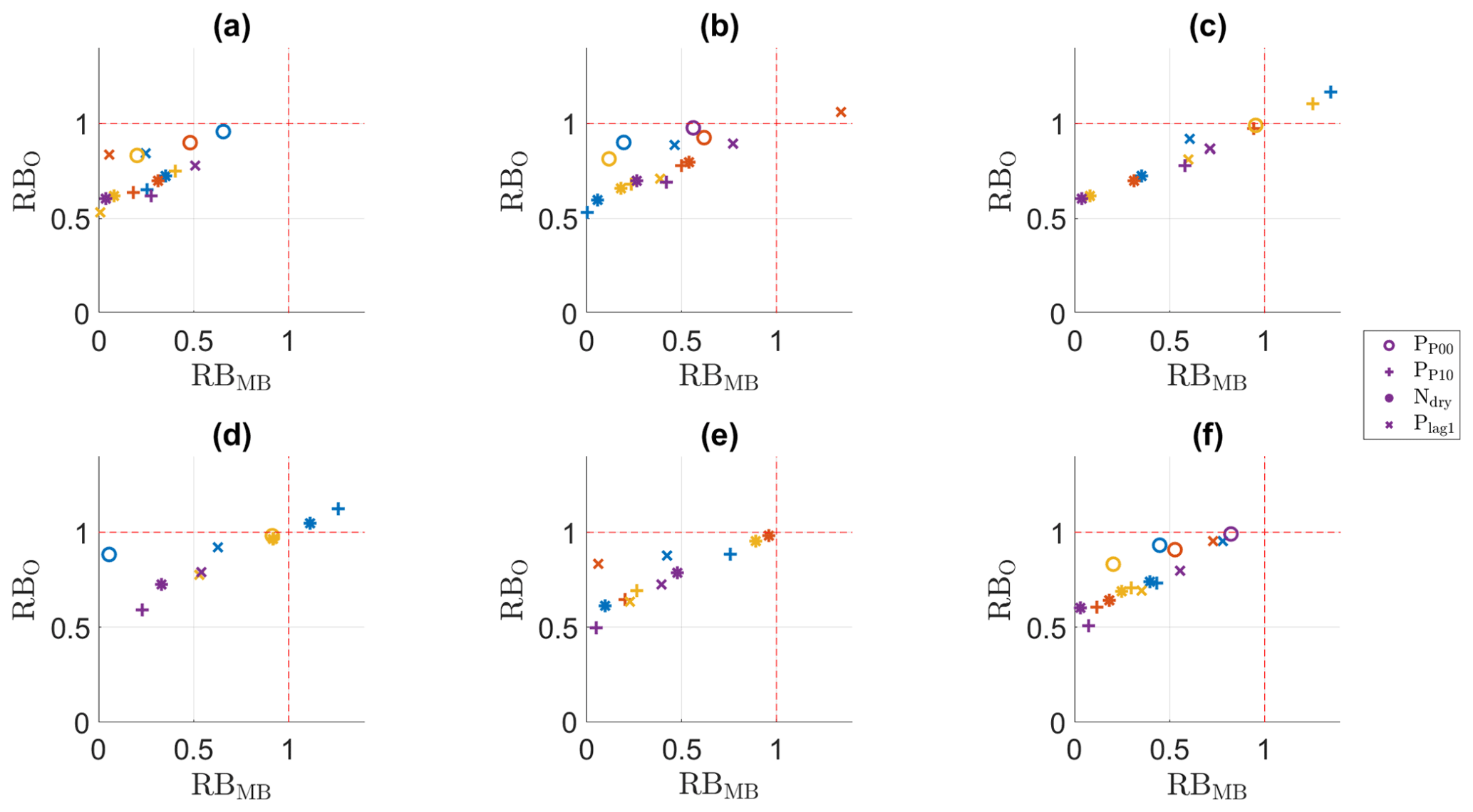
Figure 8 RB_MB versus RB₀ for the correlation indices in the validation period. (a) QDM, (b) mQDM, (c)  MBCn, (d) MRQNBC, (e) dOTC, (f) R²D². Winter: blue, spring: ochre, summer: yellow, autumn: purple.

The good performance for the validation period indicates that the impact of nonstationarity is limited, as was also shown by the small R index values (Sect. 4.1). This is confirmed by the biases in the calibration period (not shown), which are similar to those in the validation period. However, for some values, the R index value was higher than 1; thus it is important to know what caused this. For corr_E,T in summer, the differences between the validation and calibration period are limited, although only for dOTC this value is well adjusted in both periods. However, the bias for the original simulations is lower than 0.10 % in both the calibration and validation period and switches in sign, which inflates the R index value. For crosscorr${}_{E,T,\mathrm{0}}$ and crosscorr${}_{E,T,\mathrm{1}}$, the same effect occurs. Besides, it seems that the bias of these three correlations is too small to be corrected by any method and that trying to adjust this automatically inflates the results. As discussed earlier, this shows that while the R index can be a valuable tool for some variables, it does not always tell the full story.

The limited nonstationarity indicated by the R index values (most values lower than 1) and the generally good results for correlation adjustment indicate that the biases in the variables, and especially those induced by nonstationarity, will generally not propagate to the discharge by biases in the correlation. If the correlation would be biased, there would be multiple pathways for propagation: either the marginal distributions themselves (e.g., the biased large summer precipitation depth) or a mismatch between the variables (e.g., a high precipitation depth in combination with an unrealistically high evaporation).

4.6 Precipitation occurrence

Figure 9 shows that the bias-adjusting methods are able to adjust the precipitation occurrence well in most seasons. The R index values indicated that there might be some nonstationarity in spring and autumn (Sect. 4.1): the value for P_lag1 is 2, and for the other indices the values are clearly higher than those in winter and summer. In contrast to other situations of bias nonstationarity, this results in a better performance for these two seasons (calibration period not shown). Winter and summer, for which no nonstationarity could be detected, perform similarly in both the calibration and validation period. However, in all seasons mQDM (panel b) performs worse in the validation than in the calibration period. As this method uses the observed structure, the temporal structure is by construction perfect in the calibration period. The poorer result in the validation period might imply that using the observed temporal structure does not suffice for future impacts, which might be important when using delta methods for impact assessment.

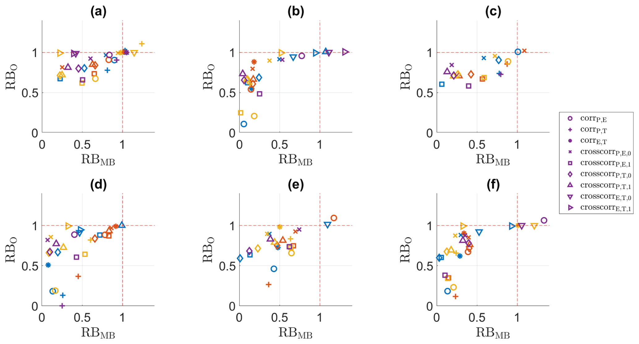
Figure 9 RB_MB versus RB₀ for the precipitation occurrence indices in the validation period. (a) QDM, (b) mQDM, (c) MBCn, (d) MRQNBC, (e) dOTC, (f) R²D². Winter: blue, spring: ochre, summer: yellow, autumn: purple.

When comparing the methods, some differences related to their structure can be noticed. In general, QDM (panel a, mQDM (panel b) and R²D² (panel f) perform best. These three methods all have the same basic structure, but this does not explain all differences with the other methods. Both MBCn (panel c) and R²D² are marginal/dependence multivariate bias-adjusting methods, but R²D² clearly performs better than MBCn for dry-to-dry transition probability. However, the methods to adjust the dependence differ: a rank-based shuffle in MBCn versus an analogue-based shuffle in R²D². It seems here that the analogue-based shuffle performs better for temporal properties. As a better temporal adjustment was one of the goals of the analogue-based shuffle (Vrac and Thao, 2020b), this is no surprise. The good performance of mQDM implies that applying the temporal structure of the observations in general still works for the “future” setting considered here. However, care should be taken when applying delta change methods on settings that are more influenced by climate change, as illustrated by the poor performance of MRQNBC. This method takes temporal aspects on different time steps into account, and it seems that this causes too much reliance on the observations. Lastly, dOTC also performs relatively well, but it is not able to correctly adjust the dry-to-dry transition probability. This poor adjustment is probably linked with one of the deficiencies of dOTC: it sometimes creates nonphysical precipitation values, which have to be corrected by thresholding.

Although some apparent bias nonstationarity was present for occurrence in spring and autumn (a high R index value for P_lag1), this did not lead to a poorer adjustment. Only some of the multivariate methods adjust the dry-to-dry transition probability poorly, but, in comparison with biases for the variables, the impact is limited. However, P_lag1 is adjusted only indirectly by the intensity adjustment. Yet, in theory this could still cause discrepancies. In general, a poor adjustment of temporal properties might lead to discharge biases by increased or decreased precipitation over a period of time, but this effect does not seem to appear in this study.

4.7 Discharge

The Perkins skill score values for discharge (Table 8) show that the application of an impact model heavily affects the biases and that the impact of bias nonstationarity can be propagated by the impact model. The general trends that were present for the marginal aspects (Tables 5–7) can no longer be distinguished. In general, the performance still decreases between the calibration and validation period, but for both winter and autumn, dOTC and R²D² perform better in the validation period than in the calibration period. Unexpectedly, MRQNBC performs best in winter and summer, but it performs worst in spring and autumn. However, given all seasons, QDM and mQDM perform best, with MBCn and R²D² performing only slightly worse. The impact of bias nonstationarity seems to be the largest in spring. All methods perform poorly in the validation period, the largest PSS value being only 65 %. In spring, evaporation was most affected by bias nonstationarity, and this seems to be propagating to the discharge PDF, despite the relatively small biases and limited influence of soil moisture on discharge in spring. The decrease in PSS value is 15 % to 20 %, depending on the method.

Table 8 PSS values for discharge in the calibration (Cal) and validation (Val) periods (%).

The RB_O and RB_MB values are shown in Figs. 10 and 11, for respectively the calibration and the validation period. The impact on the PDF for spring discharge is not clearly seen when comparing these values: for all methods and seasons, the bias adjustment seems to result in an agreeable representation of the discharge in the validation period. Yet, even a small shift can result in a poorer performance, as indicated by the PSS values.

Clearer decreases in performance can be found for summer and winter. When comparing the results for the validation period with the residual biases in the calibration period (Fig. 10), it becomes clear that the results for winter and summer are worse in the validation period. This corresponds with the poor performance for precipitation adjustment in these seasons, which was linked with bias nonstationarity. The bias-adjusting methods seem to respond similarly to the nonstationarity. For winter, the RB_O and RB_MB values are generally lower for all methods. However, only for the highest discharge percentiles (Q₉₉ and Q_99.5) and the 20-year return period index, the bias is worse after adjustment than before adjustment. This can seem negligible, but these discharge percentiles correspond with potential floods. For summer, the bias after adjustment is still lower than that of the raw climate simulations, but it has clearly increased in comparison with the calibration method. As mentioned in Sect. 4.2, it should be taken into account that the PDM calculates river discharge. The nonstationarity in summer might propagate differently when studying pluvial floods in, e.g., urban catchments. For all methods, the bias of the highest discharge percentiles was completely adjusted in the calibration period and could no longer be plotted, but it has shifted towards slightly higher RB_O and RB_MB values.

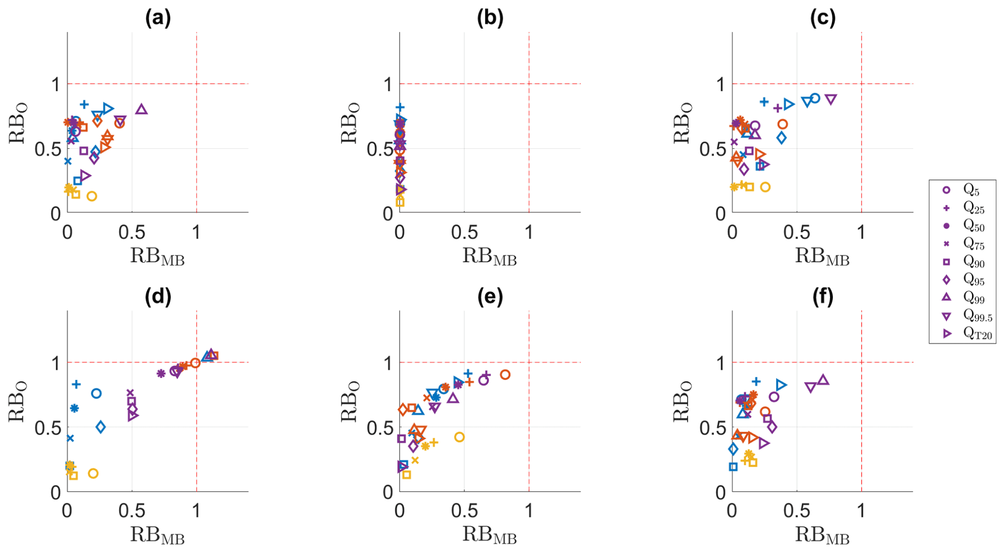
Figure 10 RB_MB versus RB₀ for the discharge percentiles and the 20-year return period value in the calibration period. (a) QDM, (b) mQDM, (c) MBCn, (d) MRQNBC, (e) dOTC, (f) R²D². Winter: blue, spring: ochre, summer: yellow, autumn: purple.

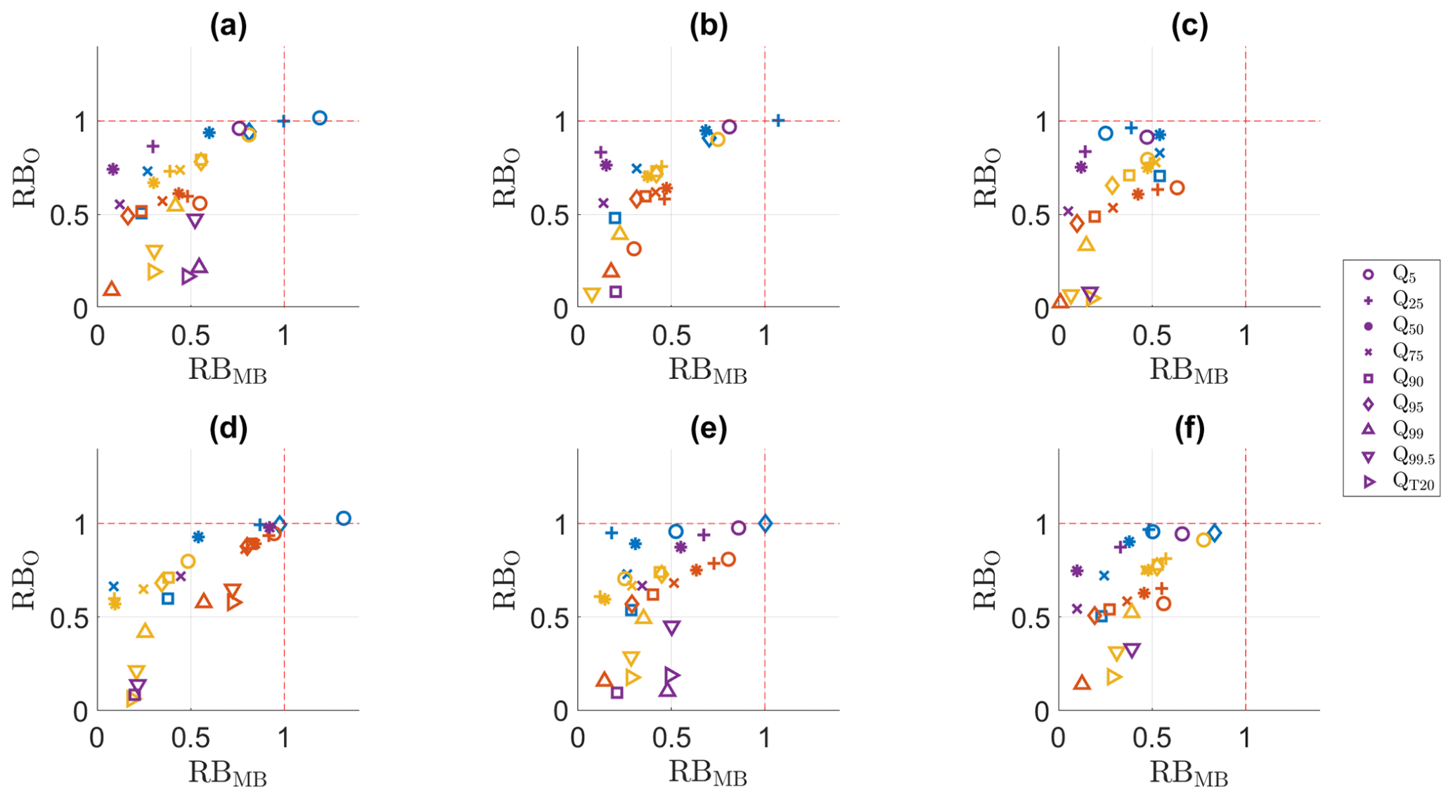
Figure 11 RB_MB versus RB₀ for the discharge percentiles and the 20-year return period value in the validation period. (a) QDM, (b) mQDM, (c) MBCn, (d) MRQNBC, (e) dOTC, (f) R²D². Winter: blue, spring: ochre, summer: yellow, autumn: purple.

In general, the results for discharge illustrate that if an important forcing variable for an impact model shows large nonstationarity, this nonstationarity will propagate through the model. There are various ways for this propagation. For example, the impact of nonstationarity on potential evaporation propagates as an influence on the PDF structure, but it is less visible when focusing on the percentiles, whereas the percentiles are more influenced by precipitation nonstationarity.

5 Discussion and conclusions

The goal of this paper was to assess how six bias-adjusting methods handle a climate change context with possible bias nonstationarity. What is presented here is only a case study for Uccle, Belgium, but the framework provided yields results that can be expanded upon. Four of the bias-adjusting methods were multivariate: MRQNBC, MBCn, dOTC and R²D². The two other ones were univariate: one was a traditional bias-adjusting method (QDM), while the other one was almost the same method but modified according to the delta change paradigm (mQDM). These univariate methods were used as a baseline for comparison. The climate change context, using 1970–1989 as calibration time period and 1998–2017 as validation time period, allowed us to calculate the change in bias between the periods, or the extent of bias nonstationarity, using the R index. The results of all methods were compared using different indices, for which the residual biases relative to the observations and model bias were calculated. Although the study was limited in spatial scale and climate models used, this yielded some results that could be valuable starting points for future research.

The calculated R index values generally demonstrated that the bias of some of these indices is not stationary under climate change conditions, although the extent of bias nonstationarity depended on the variable and index under consideration. The bias nonstationarity, as indicated by the R index (higher than 1 and often close to 2), was largest for the highest precipitation percentiles in winter and summer, for all winter temperature percentiles and the lowest temperature percentiles in spring and summer, and for evaporation percentiles in spring. The performance of all of these percentiles was clearly poorer in the validation period than in the calibration period, indicating a clear link between bias nonstationarity and poor bias adjustment performance. For both precipitation and evaporation, it could be observed that the nonstationarity propagated through the rainfall-runoff model used for impact assessment, and that the propagation was different for these variables. The precipitation nonstationarity and biases mostly affected the high discharge percentiles, whereas the evaporation biases mostly affected the full distribution.

In the context of nonstationarity, it is important to discuss how well the methods performed. Four observations could be made. As a first observation, all methods perform rather similarly, especially under nonstationarity. Although the general performance for some methods was lower depending on the studied aspect and season, as illustrated by MRQNBC and dOTC, their response to bias nonstationarity was broadly similar to other methods. That these two methods sometimes performed worse than other methods depends on the specific case. Even within this study, MRQNBC proved to be rather robust when considering discharge, although this was season-dependent.

Second, when taking everything into account, the univariate bias-adjusting methods performed best, although the difference with MBCn and R²D² was small. This was clearly illustrated by the PSS values. For the marginal aspects (P, T and E), the performance of QDM and mQDM on the one hand and MBCn and R²D² on the other hand was similar. When taking occurrence, correlation and the resulting discharge into account, the univariate methods performed slightly better. However, the methods are specifically designed to alter the marginal distributions. As already discussed in Sect. 4.5, it was pointed out by Zscheischler et al. (2019) that the multivariate bias-adjusting methods were made with other principal goals, such as spatial and dependence adjustment. As it is not assessed in this study, we cannot comment on the spatial adjustment. Nonetheless, the study by François et al. (2020) illustrated that the multivariate bias-adjusting methods can be very informative and robust for spatial adjustment. Concerning the dependence adjustment, it was shown in Sect. 4.5 that the multivariate methods all perform well for the area and model chain studied here.

Third, although the MRQNBC method performed well for dependence and precipitation, it often performed worst for temperature, evaporation, occurrence and discharge indices. MRQNBC adjusts on multiple timescales. Although this method has value, it appears to be hard to calibrate correctly. In addition, the heavy reliance on observations might exacerbate the results. This is an indication that assuming that the temporal structure of the past can be used for the future might be dangerous, as Johnson and Sharma (2011) and Kerkhoff et al. (2014) already mentioned.

Last, although the differences between MBCn and R²D² are small, the latter is better suited to take into account temporal properties. This could be seen in Fig. 9 and suggests that recent work to take into account temporal properties in bias adjustment (e.g., François et al., 2021) is worth pursuing.

The four observations listed in the previous paragraphs suggest that the choice of method should be based on the studied problem or impact type, as the impact of bias nonstationarity is much larger on the final result than differences between individual methods. The validation results could only be obtained by analyzing and comparing a broad combination of indices. Considering only the mean or other standard statistics would have hidden many of the results seen. For example, in contrast to the results for the mean, the inclusion of both high and low extremes highlighted some problems with bias nonstationarity for some variables. As such, this study does not contradict earlier studies (e.g., Maraun, 2012), where the mean-based biases were found to be rather stable. Thus, we echo the advice by Maraun and Widmann (2018a) to use indices not directly affected by bias-adjusting methods and to analyze the user needs before deciding upon the bias adjustment validation method. However, the used indices can still be improved. Although the R index provides a lot of insight into the bias nonstationarity, it has been shown to over- or underestimate the effect of bias nonstationarity depending on the size and sometimes even the sign of the original bias. Other criteria also exist, such as the “signal-to-noise ratio” (SNR) used by Hui et al. (2020). The different criteria or indices should be compared and maybe new tools are needed, so that the issue of bias nonstationarity can be more thoroughly explored.

An important limitation is that we only used one GCM–RCM combination. Using a model ensemble would be more informative but could hide a single model's poor performance, as the differences within GCM–RCM ensembles can be large (Vautard et al., 2021). Nonetheless, this study has value in illustrating possible impacts of bias nonstationarity. To broaden the scope, it helps to compare the GCM–RCM combination used in this study with the full range of EURO-CORDEX model combinations (Vautard et al., 2021). For winter temperatures, where the impact of bias nonstationarity was large, MPI-RCA4 is positively biased in the area under study, but it is not the most biased EURO-CORDEX model. In contrast, for both winter and summer precipitation, the biases in MPI-RCA4 are among the largest within the EURO-CORDEX ensemble. However, this only concerns the mean bias and conclusions can thus not be easily generalized for the extremes, where the impact of bias nonstationarity was largest. In general, the MPI-RCA4 combination does not stand out in the study of Vautard et al. (2021): it shows some biases and is thus not the best model combination, but it can not be considered to be the worst. This allows one to generalize the results seen here to other model combinations. Yet, they should still be considered on a case-by-case basis, taking into account the area under study, the studied impact, and so on. The framework presented here could be used to discard poor-performing models, based on the R index (also suggested by Maurer et al., 2013) or the remaining bias after adjustment.

To have a better view of how these results should be interpreted for impacts and compound events, the perspective of the end user should be considered (Maraun et al., 2015; Maraun and Widmann, 2018b). We used discharge as an example, using the relatively simple PDM. Even for this model, it could be observed that bias nonstationarity can propagate in multiple ways. The influence of the nonstationarity in precipitation was most clear in summer and winter. As precipitation is the driving variable for the PDM, even the limited nonstationarity, mostly in the precipitation extremes, had an influence on the discharge simulation, as could be seen for the discharge in winter and summer (Fig. 10, respectively blue and yellow). In contrast, the nonstationarity in evaporation propagated much less. However, it had an effect on the full PDF in spring, as could be observed from the PSS value for discharge (Table 8). In spring, no nonstationarity could be observed for precipitation, which allowed the influence of evaporation to be larger, although it theoretically has a smaller influence than precipitation on the discharge. The different propagation of bias nonstationarity, observed here for the extremes versus the full PDF, can be important considering that bias adjustment can be applied for many different types of impact assessment. However, the assessment in this study is relatively simple. For other impact studies, the results may vary considerably. For example, forest fires (a typical compound event, discussed in a bias adjustment context in, e.g., Yang et al., 2015, Cannon, 2018, Zscheischler et al., 2019) depend more heavily on T and E to simulate fire weather conditions. Besides such compound events, other types of application can use a wide variety of variables and, hence, the bias nonstationarity may differ. In all of these studies, the propagation of bias nonstationarity will depend on the timescales considered in the impact assessment, the timescales on which nonstationarity is present, the variables considered and the spatial scale. Although this last aspect is limited in this study, it can be assumed that if bias nonstationarity is present in one grid cell, it will also be present in neighboring grid cells with similar climatic conditions. To better understand the impact of bias nonstationarity on spatial adjustment, future work should systematically assess the performance of bias-adjustment under bias nonstationarity on a large scale. However, only a few observation-based data sets have a resolution that is comparable with that of recent RCMs, such as the ERA5-Land reanalysis (Muñoz-Sabater et al., 2021).

To conclude, the results discussed in this paper indicate that bias nonstationarity can have an important impact on the bias adjustment and the propagation of biases in impact models. Depending on the extent of nonstationarity (spatial, temporal and the variables affected), such propagation should be taken into account far more when studying future impacts. As authors have mentioned before (Ehret et al., 2012; Maraun, 2016; Nahar et al., 2017), this foremost implies that climate models have to become better at modeling the future: we need to be able to trust them as fully as possible. As long as this is not the case, bias adjustment methods have to be developed that are more robust and that are able to help us assess the future correctly. As was discussed in this paper, all methods suffer from bias nonstationarity, increasing the uncertainty of future impacts.