The effects of spatial and temporal resolution of gridded meteorological forcing on watershed hydrological responses

Meteorological forcing plays a critical role in accurately simulating the watershed hydrological cycle. With the advancement of high-performance computing and the development of integrated watershed models, simulating the watershed hydrological cycle at high temporal (hourly to daily) and spatial resolution (tens of meters) has become efficient and computationally affordable. These hyperresolution watershed models require high resolution of meteorological forcing as model input to ensure the fidelity and accuracy of simulated responses. In this study, we utilized the Advanced Terrestrial Simulator (ATS), an integrated watershed model, to simulate surface and subsurface flow and land surface processes using unstructured meshes at the Coal Creek Watershed near Crested Butte (Colorado). We compared simulated watershed hydrologic responses including streamflow and distributed variables such as evapotranspiration, snow water equivalent (SWE), and groundwater table driven by three publicly available, gridded meteorological forcings (GMFs) – Daily Surface Weather and Climatological Summaries (Daymet), the Parameter-elevation Regressions on Independent Slopes Model (PRISM), and the North American Land Data Assimilation System (NLDAS). By comparing various spatial resolutions (ranging from 400 m to 4 km) of PRISM, the simulated streamflow only becomes marginally worse when spatial resolution of meteorological forcing is coarsened to 4 km (or 30 % of the watershed area). However, the 4 km-resolution has much worse performance than finer resolution in spatially distributed variables such as SWE. Using the temporally disaggregated PRISM, we compared models forced by different temporal resolutions (hourly to daily), and sub-daily resolution preserves the dynamic watershed responses (e.g., diurnal fluctuation of streamflow) that are absent in results forced by daily resolution. Conversely, the simulated streamflow shows better performance using daily resolution compared to that using sub-daily resolution. Our findings suggest that the choice of GMF and its spatiotemporal resolution depends on the quantity of interest and its spatial and temporal scale, which may have important implications for model calibration and watershed management decisions.

1 Introduction

The accuracy of meteorological forcings such as precipitation plays a crucial role in simulating the watershed hydrological cycle. With the advancement of high-performance computing and the development of integrated hydrologic models (e.g., Amanzi-Advanced Terrestrial Simulator – ATS Coon et al., 2019, ParFlow, Kollet and Maxwell, 2006, and HydroGeoSphere, Aquanty, 2015), simulating the watershed hydrological cycle at high temporal and spatial resolution has become possible (Wood et al., 2011). These models often require gridded meteorological forcing (GMF), which is typically fused from various sources, including ground-based gages, radar, satellite remote sensing, as well as regional and global climate models. Due to different interpolation methods and data sources, GMF is available at different spatial and temporal resolutions and contains considerable uncertainties (Schreiner‐McGraw and Ajami, 2020).

Recently, GMF products, notably Daily Surface Weather and Climatological Summaries (Daymet) (Thornton et al., 1997, 2021), the Parameter-elevation Regressions on Independent Slopes Model (PRISM) (Daly et al., 2008), and the North American Land Data Assimilation System (NLDAS) (Mitchell, 2004; Xia et al., 2012)), have become popular for hydrologic modeling within the conterminous United States (CONUS) owing to their temporally and spatially complete coverage and relatively high spatiotemporal resolution. Past studies have compared and evaluated the performance of GMF against weather stations (Behnke et al., 2016; Daly et al., 2008; Muche et al., 2020). Daly et al. (2008) presented a detailed comparison between PRISM and Daymet and found that, for the products available in 2008, PRISM outperforms Daymet, especially in mountainous and coastal areas of the western US. Behnke et al. (2016) compared eight widely used meteorological forcing datasets, including Daymet, PRISM, and NLDAS against Global Historical Climatology Network-Daily (GHCN-D) stations across the CONUS. They found that different interpolation methods affected the accuracy of downscaled meteorological data, and care should be taken when selecting meteorological forcing for a given region. In a similar study, Muche et al. (2020) compared four GMFs (i.e., Daymet, PRISM, NLDAS, and the Global Land Data Assimilation System – GLDAS) as precipitation data sources and evaluated the precipitation estimates at GHCN-D stations within the Delaware Watershed at Perry Lake in eastern Kansas. They showed that precipitation from Daymet and PRISM were more closely matched with precipitation collected at GHCN-D than that from NLDAS and GLDAS.

Understanding the bias and fidelity of each meteorological forcing and the effects of meteorological forcing spatiotemporal resolution on simulated watershed responses is important for accurate simulations of watershed processes. Previous studies have evaluated the impact of different GMFs on model-simulated surface runoff (Muche et al., 2020; Behnke et al., 2016; Gao et al., 2017; Elsner et al., 2014). Using the Soil and Water Assessment Tool (SWAT), Muche et al. (2020) evaluated model performance on simulated streamflow against observation under different GMFs. They found that the simulated streamflow yielded a higher correlation when driven by PRISM and Daymet than those by NLDAS and GLDAS. Eum et al. (2014) evaluated hydrologic responses using the Variable Infiltration Capacity (VIC) model forced by three GMFs available in Canada. They found notable differences in simulated surface runoff during the snowmelt period but not so much during the snowfall period. However, these studies mostly focused on meteorological forcing effects on surface runoff and ignored other relevant hydrological processes (e.g., snowmelt, evapotranspiration – ET –, and subsurface flow). In addition, these studies used either semi-distributed models (e.g., SWAT) or coarse regional-scale land surface models (e.g., VIC), which do not fully utilize the GMFs at their finest resolutions.

Compared to semi-distributed models, fully distributed, integrated hydrologic models are favorable in simulating watershed hydrologic responses to changes in climate forcing as they can preserve the spatial heterogeneity of inputs from GMF and provide a spatially distributed representation of both surface and subsurface flow processes. Recently, Maina et al. (2020) used the ParFlow-Community Land Model (CLM), a fully distributed, process-based watershed model, to study the effect of spatial resolution of meteorological forcing (0.5 to 40.5 km) generated from the Weather Research and Forecasting (WRF) model on spatially resolved hydrologic responses, including snow water equivalent (SWE), ET, infiltration, surface ponded depth, and groundwater table. Using the Cosumnes Watershed as a test bed, they found that most hydrologic variables were seasonally and spatially dependent on the different spatial resolutions of the meteorological forcing. Although climate models such as WRF provide alternative GMF at any given spatiotemporal resolution, they require extensive expert knowledge in setting up and running the models and thus are less popular compared to publicly available GMFs (e.g., Daymet, PRISM, and NLDAS). To our knowledge, few, if any, studies have utilized the common GMFs to investigate the impact of spatial resolution of meteorological forcing on both watershed cumulative variables (e.g., streamflow) and distributed variables (e.g., SWE, ET, and groundwater level).

The temporal resolution of meteorological forcing, especially precipitation, plays an important role in the timing of runoff generation. It is particularly important for flood volume modeling (Ficchì et al., 2016), flood forecasting (Wetterhall et al., 2011), and hydrodynamic modeling in urban catchments (Ochoa-Rodriguez et al., 2015; Bruni et al., 2015). The temporal resolution of rainfall inputs has been shown to affect the simulation of surface runoff more strongly than variations in spatial resolution during storm events (Ochoa-Rodriguez et al., 2015). High temporal resolution is also important for studying watershed biogeochemical cycling since sub-daily meteorological forcing could induce diurnal snowmelt that produces regular infiltration of cold, chemically distinct snow water into the soil which alters the soil temperature and chemical composition of soil water and groundwater (Petrone et al., 2007; Woelber et al., 2018). Despite the importance of the temporal resolution of input forcing, the impact of GMF temporal resolution on watershed hydrodynamics has largely been overlooked. For example, a daily timestep is used routinely in watershed hydrologic modeling, and the simulated daily streamflow is generally used to compare to observed daily streamflow even though sub-daily streamflow measurement is collected at most United States Geological Survey (USGS) stream gages.

The objectives of this study are to intercompare three widely available GMFs (i.e., PRISM, Daymet, and NLDAS) and to evaluate the impact of meteorological forcing spatial and temporal resolution on simulated watershed hydrologic responses including streamflow, ET, SWE, soil moisture, ponded surface water depth, and groundwater table. We choose ATS as the integrated watershed model to couple surface and subsurface flows with land surface processes (Coon et al., 2019). The model can fully resolve the meteorological forcing at a much finer resolution (≤100 m) using unstructured triangular grids. We seek to understand the impact of meteorological forcing by comparing model simulations to field observations including GHCN-D stations, USGS stream gages, and remote-sensing products. We aim to answer the following questions.

1. How would different GMFs at their native resolutions impact the simulated streamflow, distributed variables such as SWE?

2. What are the effects of spatial and temporal resolution of GMF on simulated streamflow and spatially distributed variables?

3. Is spatial resolution more important than temporal resolution of the GMF for watershed hydrologic simulations?

To address these questions, we perform different numerical experiments using ATS by forcing the model with various spatial and temporal resolutions of GMFs. We choose a mountainous watershed due to its complex terrain and heterogeneous weather conditions, which provides an ideal test bed for studying the impact of meteorological forcing spatiotemporal resolution on watershed dynamic responses. The findings from this study are relevant for the use of the GMF dataset in watershed hydrologic simulations using fully distributed watershed models in mountainous watersheds. It also provides important implications for watershed calibration using inverse modeling.

2 Methods

2.1 Study site

Our study site is located in the Coal Creek Watershed (Hydrologic Unit Code (HUC) 140200010204) with an area of 53.2 km² located within the larger East Taylor Watershed (HUC 14020001) near Crested Butte, in southwestern Colorado (Fig. 1). The Coal Creek Watershed is a high alpine, snow-dominated catchment, characterized as warm summer, humid continental climate in the Köppen classification system (Koppen and Geiger, 1930). It receives ∼850 mm of precipitation annually, with ∼530 mm as snowfall which was estimated from the long-term Daymet forcing dataset (Thornton et al., 2021). The primary land cover types are evergreen forest (62.6 %) and shrub (20.5 %). This watershed has strong variations in topography and land cover, which is representative of many headwater, mountainous watersheds in the western US.

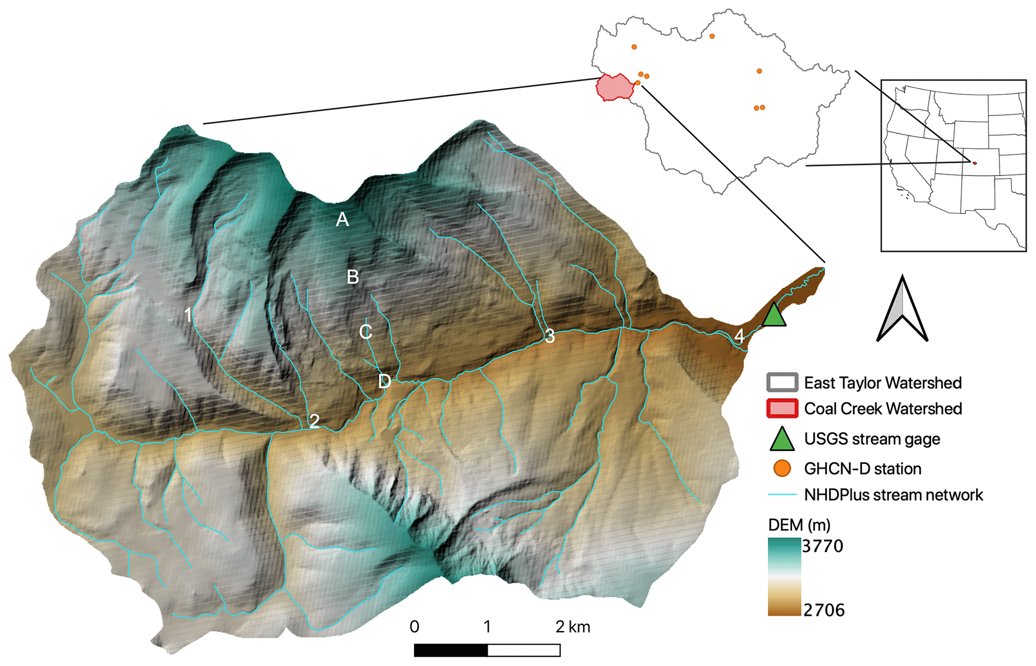
Figure 1 Map of the Coal Creek Watershed in relation to the larger East Taylor Watershed as well as its relative location in the western US. Also shown are the locations of GHCN-D stations, the USGS stream gage, the National Hydrography Dataset Plus (NHDPlus) stream network, and the digital elevation model (DEM). The marked points (A–D) and (1)–(4) are point locations used to observe groundwater table and surface ponded depth from the model, respectively.

2.2 ATS model setup

ATS is an integrated, distributed hydrologic code that solves the diffusion wave approximation of the St-Venant equations for surface flow coupled to the Richards equation for flow in variably saturated porous media in the subsurface (Coon et al., 2019, 2020). The Richards equation is described as

$$\begin{array}{}\text{(1)}& {\displaystyle \frac{\partial }{\partial t}}\left(\mathit{\varphi }s\right)+\mathit{▿}\cdot q=\mathrm{0},\end{array}$$

with

$$\begin{array}{}\text{(2)}& q=-{\displaystyle \frac{\mathrm{1}}{\mathit{\mu }}}{k}_{\mathrm{r}}\mathit{\kappa }(\mathit{▿}p+\mathit{\rho }g),\end{array}$$

where ϕ is the effective porosity (–), s is the saturation (–), q is the Darcy flux (m s⁻¹), μ is the dynamic viscosity (Pa s⁻¹), k_r is the relative permeability (–), κ is the saturated hydraulic permeability (m²), p is the water pressure (Pa), and g is the gravitational constant (m s⁻²).

The diffusive wave approximation to overland flow is described as

$$\begin{array}{}\text{(3)}& {\displaystyle \frac{\partial h}{\partial t}}+\mathit{▿}\cdot \left(hv\right)=Q_{\mathrm{w}}+Q_{\mathrm{ss}},\end{array}$$

with

$$\begin{array}{}\text{(4)}& v=-{\displaystyle \frac{h^{\mathrm{2}/\mathrm{3}}}{n\cdot \max \left(\mathit{ϵ},\sqrt{\mathit{▿}z}\right)}}\mathit{▿}(z+h),\end{array}$$

where h is the depth of ponded water (m), v is the surface flow velocity (m s⁻¹), Q_w are all external source/sink terms (m s⁻¹), Q_ss is the exchange flux between surface and subsurface systems (m s⁻¹), n is Manning's coefficient (s m${}^{-\mathrm{1}/\mathrm{3}}$), z is surface elevation (m), and ϵ is a small positive regularization to keep the equations non-singular in places with zero bed slope (m).

The ATS meshes including surface land covers and subsurface structures and properties were developed using the Watershed Workflow package (Coon and Shuai, 2021), which brings together a variety of data streams, delineates the catchment, and generates a variable-resolution mesh with refined resolution at the stream network. Resolutions ranged from typical triangle areas of 5000 m² near the stream network to 50 000 m² away from the stream network. This triangular surficial mesh was then elevated using a digital elevation model (DEM) from the USGS National Elevation Dataset (NED) 30 m resolution dataset.

On the surface, 14 land cover types were delineated from the National Land Cover Database (NLCD 2016) product for the CONUS. The leaf area index (LAI) seasonal variations for each land cover type were retrieved from MODIS (https://modis.gsfc.nasa.gov/data, last access: 31 March 2021). Some of the plant functional types and their properties such as rooting profile and photosynthetic parameters were adopted from parameters used in the CLM 4.5 technical notes (Oleson et al., 2013).

In the subsurface, the model was discretized into 19 terrain-following layers with a total thickness of ∼28 m. A total of six soil layers encompassed the top 2 m of the domain. The depth to bedrock (DTB) was determined from SoilGrids (Shangguan et al., 2017) that varies from 3 m at its shallowest to 26 m at its deepest. The geologic layers were sandwiched between the soil and bedrock layers. The vertical resolution of the mesh gradually increased from 5 cm at the surface to 2 m at the 2 m depth, and it remained constant at 2 m until the bottom of the model domain at a depth of 28 m. The total number of cells is 171 760.

Based on the National Resources Conservation Service (NRCS) Soil Survey Geographic (SSURGO) soils database, 22 soil types were identified and mapped within the soil layer. Due to the edge-matching issues in the SSURGO soil database (Gatzke et al., 2011), the 22 soil types were regrouped into 9 types to remove the discontinuity of a soil type across soil survey area boundaries. Using a global surface geology dataset from GLobal HYdrogeology MaPS (GLHYMPS) 2.0 (Huscroft et al., 2018), 11 geologic material types were identified and mapped within the geologic layer. The spatial distribution of the soil and geological layers was shown in Fig. 2. The permeability and porosity for each soil type were retrieved from the SSURGO database, and the van Genuchten parameters were determined using Rosseta v3, a pedotransfer function that relates sand, silt, and clay percentage to van Genuchten parameters (Zhang and Schaap, 2017). The permeability and porosity for each geology type were retrieved from the GLHYMPS database. Bedrock functions as a confining layer and is assumed to have a very small permeability of $\mathrm{1}\times {\mathrm{10}}^{-\mathrm{17}}$ m².

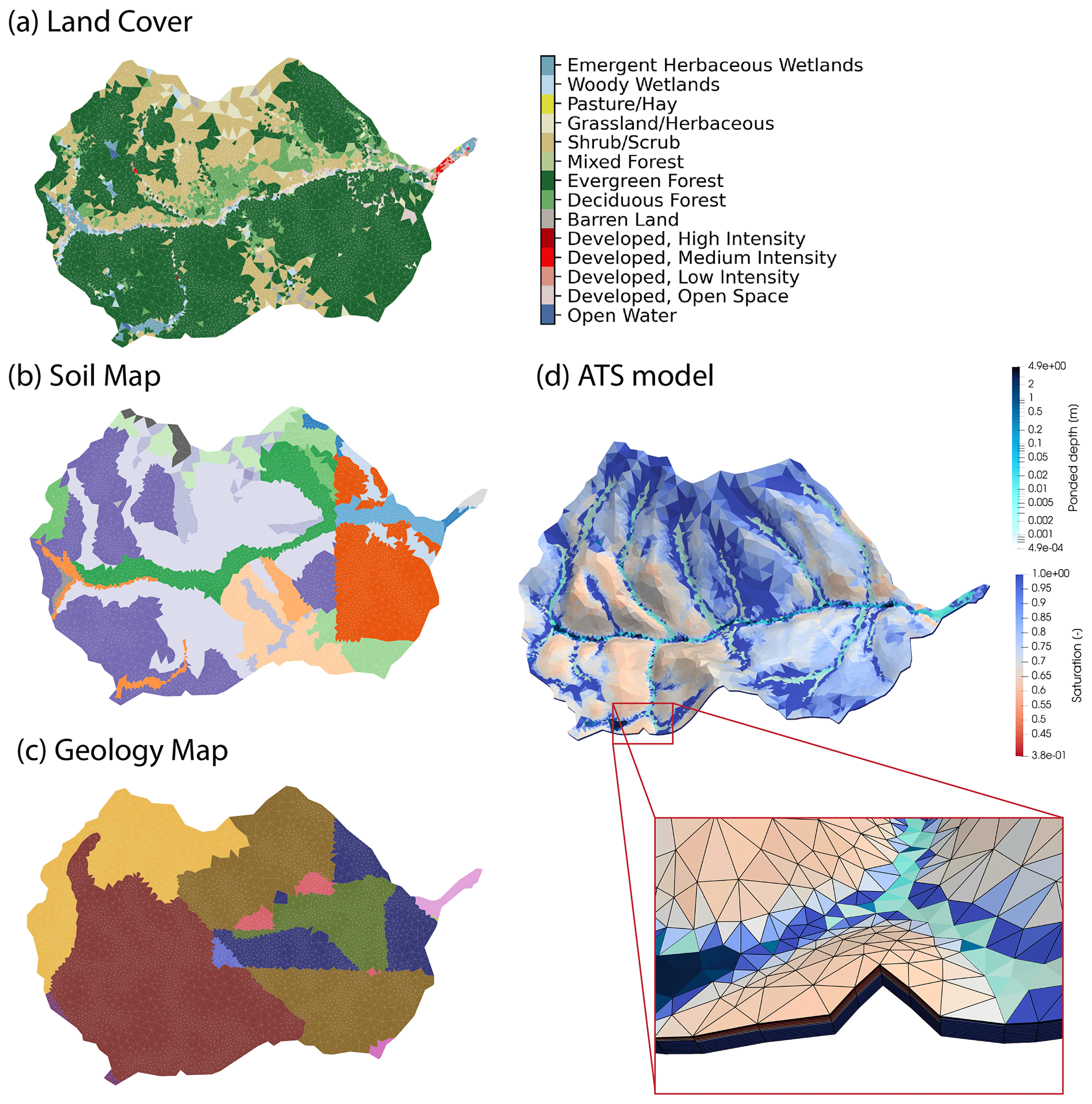
Figure 2 (a) Land cover, (b) soil map, and (c) geology map of Coal Creek Watershed that are generated from Watershed Workflow. (d) ATS-simulated surface ponded depth and soil saturation on 1 October 2018. The zoomed-in plot shows the 3D unstructured triangular mesh.

The model was first run for 1000 years with constant precipitation (∼850 mm yr⁻¹) as the cold spinup that resulted in steady-state model outputs at the final timestep, which was then used as the initial condition for a 10-year (1 October 2004–1 October 2014) transient simulation (i.e., warm spinup) driven by the Daymet forcing. Model state at the end of the 10-year run was used as the initial condition for a 4-year transient run (1 October 2015–1 October 2019) driven by various GMFs. The water year 2015 was treated as a second warm spinup and was discarded from the analysis to avoid any influence from previous spinup runs. The study period features a high snow year (∼709 mm in water year 2017) and a low snow year (∼296 mm in water year 2018), allowing us to demonstrate how different meteorological forcings impact watershed responses under various weather conditions. ATS runs were taken at a sub-hourly timestep determined by the model while outputting streamflow and watershed-averaged variables at an hourly timestep. Due to large file size, spatially distributed variables such as SWE and ET were output at daily timesteps. Each run took ∼17 h wall-clock time using 64 processors on the Cori clusters at the National Energy Research Scientific Computing Center (NERSC). The models were not calibrated because the focus of this study was to evaluate the effect of meteorological forcings on model simulation instead of estimating the optimal parameters used in ATS.

2.3 Gridded meteorological forcing

For this comparison, three widely used GMFs were considered: PRISM (Daly et al., 2008), NLDAS-2, (Xia et al., 2012)), and Daymet v4 (Thornton et al., 1997, 2021). NLDAS-2 and Daymet v4 are hereafter referred to as NLDAS and Daymet, respectively. The detailed comparison between each meteorological dataset can be found in Table 1.

(Thornton et al., 1997)(Daly et al., 2008)(Cosgrove et al., 2003)

Table 1 Meteorological dataset comparison.

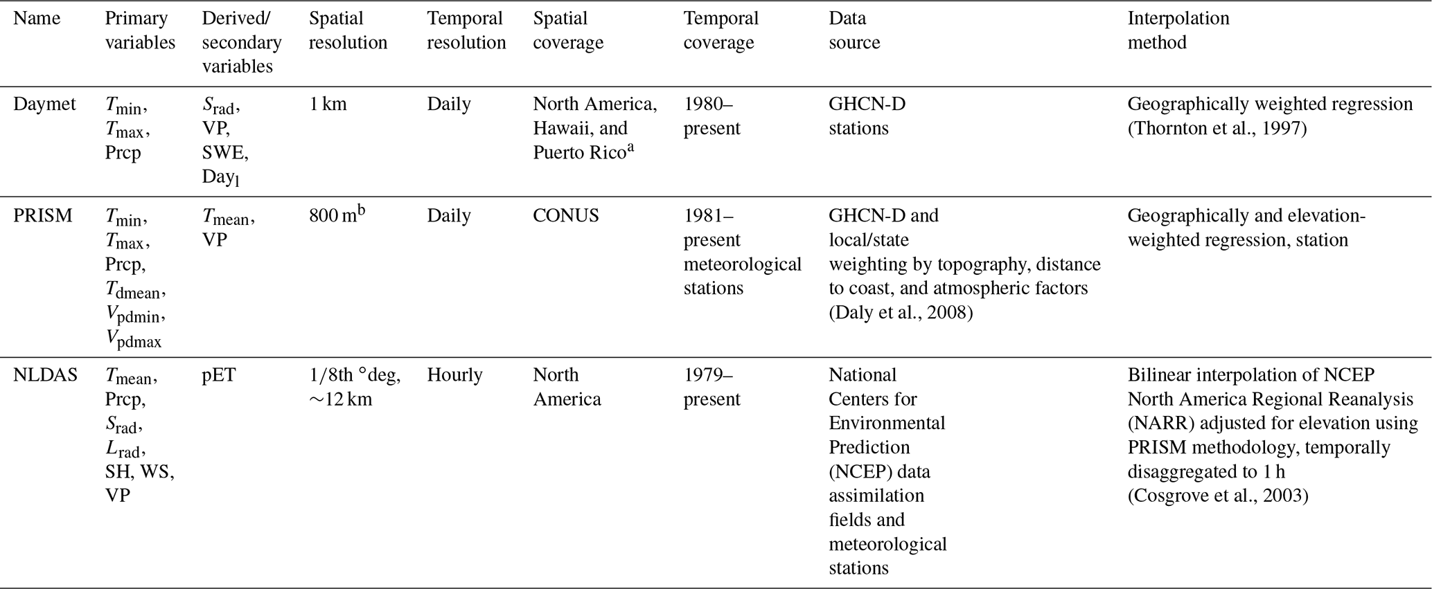
Abbreviations: T_min: minimum temperature, T_max: maximum temperature, T_mean: mean temperature, Prcp: precipitation, S_rad: shortwave radiation, L_rad: longwave radiation, VP: vapor pressure, SWE: snow water equivalent, Day_l: day length, T_dmean: mean dew point temperature, V_pdmin: minimum vapor pressure deficit, V_pdmax: maximum vapor pressure deficit, SH: specific humidity, WS: wind speed, pET: potential evaporation. ^a Puerto Rico has had Daymet since 1950. ^b This native resolution is not free.

The Daymet climate forcing is a gridded, daily product with a spatial resolution of 1 km, covering continental North America, Puerto Rico, and Hawaii. It assimilates data from weather stations (primarily GHCN-D stations) and accounts for elevation, prevailing winds, storm tracks, and proximity to large water bodies (Thornton et al., 1997). Here, the latest Daymet version 4 product is used because this product has gone through significant bias corrections in station observations and the gridded product shows a better match with weather stations compared to the earlier versions (Thornton et al., 2021).

The PRISM forcing is developed by the PRISM climate group at Oregon State University and is recognized as the official climate dataset for the US Department of Agriculture. It utilizes a wide range of monitoring networks including GHCN-D stations and local/state weather stations to generate daily, spatially continuous climate data for the CONUS. PRISM provides a native grid resolution of 30 arcsec (∼800 m) for a fee but also provides a coarsened 4 km resolution free of charge. We used the native 30 arcsec resolution and downscaled (upscaled) the dataset to obtain finer (coarser) spatial resolutions.

The NLDAS dataset is a gridded, hourly product with a spatial resolution of $\mathrm{1}/\mathrm{8}$th^∘ (∼12 km at the study site) for the entire North American region. The non-precipitation forcing variables are primarily derived from the North American Regional Reanalysis (NARR) by spatially interpolating data from the 32 km-resolution NARR grid to the $\mathrm{1}/\mathrm{8}$th^∘ NLDAS grid while temporally disaggregated from 3-hourly to hourly frequency (Cosgrove et al., 2003). The precipitation is a product of a temporal disaggregation of a gage-only Climate Prediction Center (CPC) analysis of daily precipitation into hourly frequency, performed directly on the NLDAS grid and including an orographic adjustment based on the widely applied PRISM climatology.

All three datasets provide temperature and precipitation as the primary forcing with a few secondary forcing variables. In addition to temperature and precipitation, ATS requires solar radiation (both incoming shortwave radiation (S_rad) and longwave radiation – L_rad), relative humidity, and wind speed as forcing inputs. Relative humidity can be estimated based on vapor pressure and mean temperature (Bolton, 1980). L_rad can be estimated from S_rad and relative humidity. Because PRISM does not provide S_rad and L_rad, we used solar radiation from Daymet instead. Wind speed was assumed to be constant (i.e., 4 m s⁻¹) for both Daymet and PRISM. Compared to PRISM and Daymet, NLDAS provides the most complete set of variables to drive ATS simulations.

Different meteorological forcings have different definitions for a calendar day, and they are often different from the local time used in the observation data (see Table A1 in the Appendix). Time zone adjustment and lag corrections have been applied to account for the time lag difference between meteorological forcing and local gages. For example, PRISM lags Daymet by 1 d, so PRISM has been shifted forward 1 d to be consistent with Daymet. Both model simulation and gage observation have been converted to the Coordinated Universal Time (UTC) time zone for hourly streamflow comparison. For consistency, all simulated streamflows are in hourly resolution and are compared to hourly USGS streamflows in Sect. 3.

To study the effect of spatial resolution of meteorological forcing, precipitation and temperature from 800 m PRISM and 1 km Daymet have been downscaled (upscaled) into finer (coarser) spatial resolutions. The downscaling of 800 m PRISM or 1 km Daymet into 400 m used a data-driven downscaling approach (Mital et al., 2022). Specifically, random forests (Breiman, 2001) were used to extract the relationships between precipitation (or average temperature) and topography. These relationships were developed at 800 m (for PRISM) and 1 km (for Daymet) resolutions and were used as-is to generate the 400 m downscaled estimates. The downscaled precipitation grids were additionally filtered to ensure a smooth field in low-gradient areas without affecting high-gradient areas (Daly et al., 2008). The topographic variables considered were elevation, slope, aspect, latitude, and longitude. These variables were extracted from the NED 10 m-resolution product and upscaled to 400 and 800 m (for PRISM) via bilinear interpolation. Upscaling of topographic variables was done in maximum increments of 2× (e.g., 10 m → 20 m → 40 m and so on).

For consistency, spatial upscaling of 800 m PRISM into 1600 and 4000 m was performed using a coarsened function from python package xarray (http://xarray.pydata.org, last access: 1 April 2021) by applying a moving average based on a 2×2 window size. The same approach was used for spatial upscaling of 1 km Daymet to 2 and 4 km. To study the effect of temporal resolution of meteorological forcing, the daily PRISM dataset was disaggregated into hourly resolution using the temporal pattern of NLDAS. The hourly PRISM dataset was then aggregated into 12-hourly temporal resolution by taking the mean (for temperature) or sum (for precipitation) for the aggregated period.

In ATS, meteorological forcing is distributed linearly across its temporal resolution, and each model surface cell gets its meteorological forcing through spatially bilinear interpolation. For example, both Daymet and PRISM apply their meteorological forcing at the daily timescale, whereas NLDAS applies its meteorological forcing at an hourly timescale.

2.4 Observation data

Instantaneous streamflow data (every 15 min) have been available from 1 April through 15 November every year since 2014 at a USGS gage (station number 09111250) located at the watershed outlet. The 15 min streamflow was aggregated to hourly streamflow which was used to compare against model simulations in the Results section. Past Airborne Snow Observatory (ASO) survey has four flights covering this watershed in 2018 and 2019 to survey the snow depth and SWE. Remote sensing products such as the Moderate Resolution Imaging Spectroradiometer (MODIS) 8 d composite ET have been available at a 500 m resolution since 2000. Groundwater measurements and field-observed soil moisture data are not available within the study site.

To compare the accuracy of each meteorological forcing against field observations, all three meteorological forcings at their native resolutions were compared against GHCN-D weather stations within the East Taylor Watershed. In total, there were seven stations with long-term precipitation records and four stations with long-term temperature records (see GHCN-D station locations in Fig. 1). Both precipitation and temperature time series were extracted at each GHCN-D gage location from the GMF.

2.5 Model evaluation metrics

Model-simulated outputs were compared against observation data including hourly streamflow from a USGS gage and spatially distributed SWE from the ASO survey. The modified Kling–Gupta efficiency (KGE) and its three components (r, γ, β) were used to evaluate the model performance (Kling et al., 2012) in addition to the standard Nash–Sutcliffe efficiency (NSE). The theoretical version of the modified KGE metric is

$$\begin{array}{}\text{(5)}& \mathrm{KGE}=\mathrm{1}-\sqrt{(r-\mathrm{1}{)}^{\mathrm{2}}+(\mathit{\gamma }-\mathrm{1}{)}^{\mathrm{2}}+(\mathit{\beta }-\mathrm{1}{)}^{\mathrm{2}}},\end{array}$$

with

$$\begin{array}{}\text{(6)}& r={\displaystyle \frac{\mathrm{cov}(S,O)}{{\mathit{\sigma }}_{\mathrm{s}}{\mathit{\sigma }}_{\mathrm{o}}}},\end{array}$$

$$\begin{array}{}\text{(7)}& {\displaystyle }& {\displaystyle }\mathit{\gamma }={\displaystyle \frac{{\mathit{\sigma }}_{\mathrm{s}}/{\mathit{\mu }}_{\mathrm{s}}}{{\mathit{\sigma }}_{\mathrm{o}}/{\mathit{\mu }}_{\mathrm{o}}}},\text{(8)}& {\displaystyle }& {\displaystyle }\mathit{\beta }={\displaystyle \frac{{\mathit{\mu }}_{\mathrm{s}}}{{\mathit{\mu }}_{\mathrm{o}}}},\end{array}$$

where S and O represent simulated and observed values, respectively, r is the correlation coefficient, γ is the variability ratio, β is the bias ratio, cov(S,O) is the covariance between simulated and observed values, σ is the standard deviation, and μ is the mean.

Using the modified KGE avoids the effect of input bias on the variability indicator, which has an advantage over the original KGE (Gupta et al., 2009; Kling et al., 2012), and it also allows diagnostic interpretation of the performance score. KGE decomposes model performance into correlation (r), variability (γ), and bias (β) terms. For example, the correlation measures the temporal dynamics of streamflow (i.e., timing), while the variability and bias measure the flow duration curve (i.e., magnitude). The KGE ranges from −∞ (poorest model skill) to 1 (perfect) when all three terms reach unity. Similarly, the NSE ranges from −∞ (poorest model skill) to 1 (perfect).

A Taylor diagram is used to show how closely a set of patterns (e.g., meteorological forcing) matches observations (Taylor, 2001). In each Taylor diagram, performance metrics such as standard deviation and Pearson's correlation coefficient (r) are shown together. The azimuthal angle represents correlation, and the radial distance represents the standard deviation. Also shown is the centered root mean square error (RMSE) between simulation and observation. The relationship between these statistics is shown below:

$$\begin{array}{}\text{(9)}& E^{\mathrm{2}}={\mathit{\sigma }}_{\mathrm{s}}^{\mathrm{2}}+{\mathit{\sigma }}_{\mathrm{o}}^{\mathrm{2}}-\mathrm{2}{\mathit{\sigma }}_{\mathrm{s}}{\mathit{\sigma }}_{\mathrm{o}}r,\end{array}$$

where E is the centered RMSE, which is also measured by the geometric distance between simulation and observation data points on the Taylor diagram (unit is the same as the standard deviation). In cases where more than one observation point are plotted on the same diagram, the centered RMSE is omitted. Note that the centered RMSE is a mean-removed RMSE, and thus any bias in the data is not shown.

The closer the distance between simulation and observation data point on a Taylor diagram, the smaller the centered RMSE (observation data point has centered RMSE=0), the more similarity they show in terms of standard deviation, and the higher the correlation coefficient (observation data point has r=1).

3 Results

3.1 Comparison between meteorological forcing and weather stations

A Taylor diagram was used to compare the similarity in precipitation and temperature patterns between meteorological forcing and GHCN-D stations (Fig. 3). Compared to temperature, precipitation showed stronger spatial heterogeneity among stations indicated by the larger difference in standard deviation and correlation. The close clustering of temperature data points indicated that the difference between different stations in temperature patterns was small. For precipitation, PRISM showed a strong correlation (r>0.9) with GHCN-D at three stations, whereas Daymet only showed a strong correlation at one location and all NLDAS sites showed a relatively weak correlation ($\mathrm{0.5}<r<\mathrm{0.85}$). For temperature, all three meteorological forcings showed a very strong correlation (r>0.95) with GHCN-D, though Daymet was slightly better than PRISM and NLDAS. Previous studies also reported similar findings at different watersheds that Daymet and PRISM showed better agreement with ground-based observational data than NLDAS (Muche et al., 2020), and the temperature was more accurately represented than precipitation (Behnke et al., 2016).

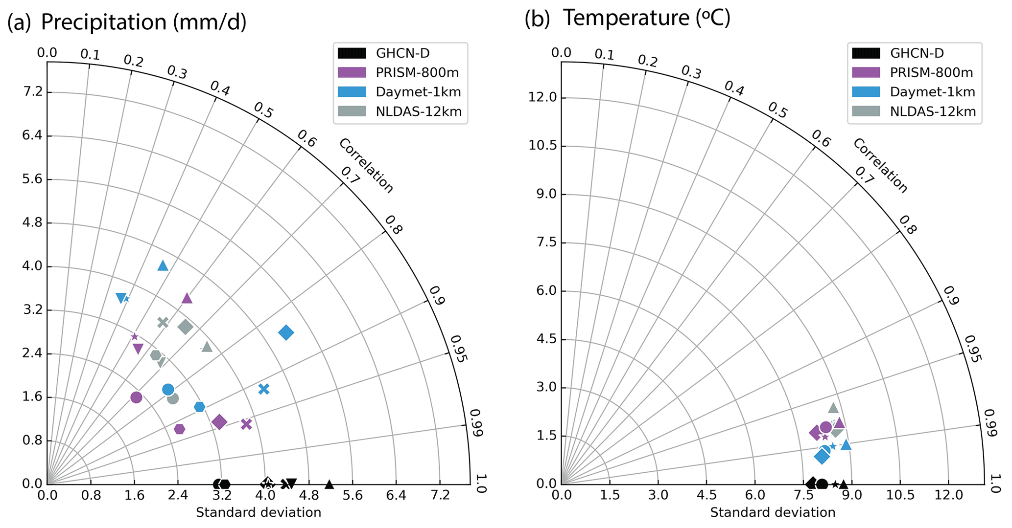
Figure 3 Taylor diagram showing the correlation coefficients and standard deviations between meteorological forcing and GHCN-D gages (black) for (a) precipitation and (b) temperature. The azimuthal angle represents correlation, and the radial distance represents the standard deviation. Each marker symbol represents a different GHCN-D station location.

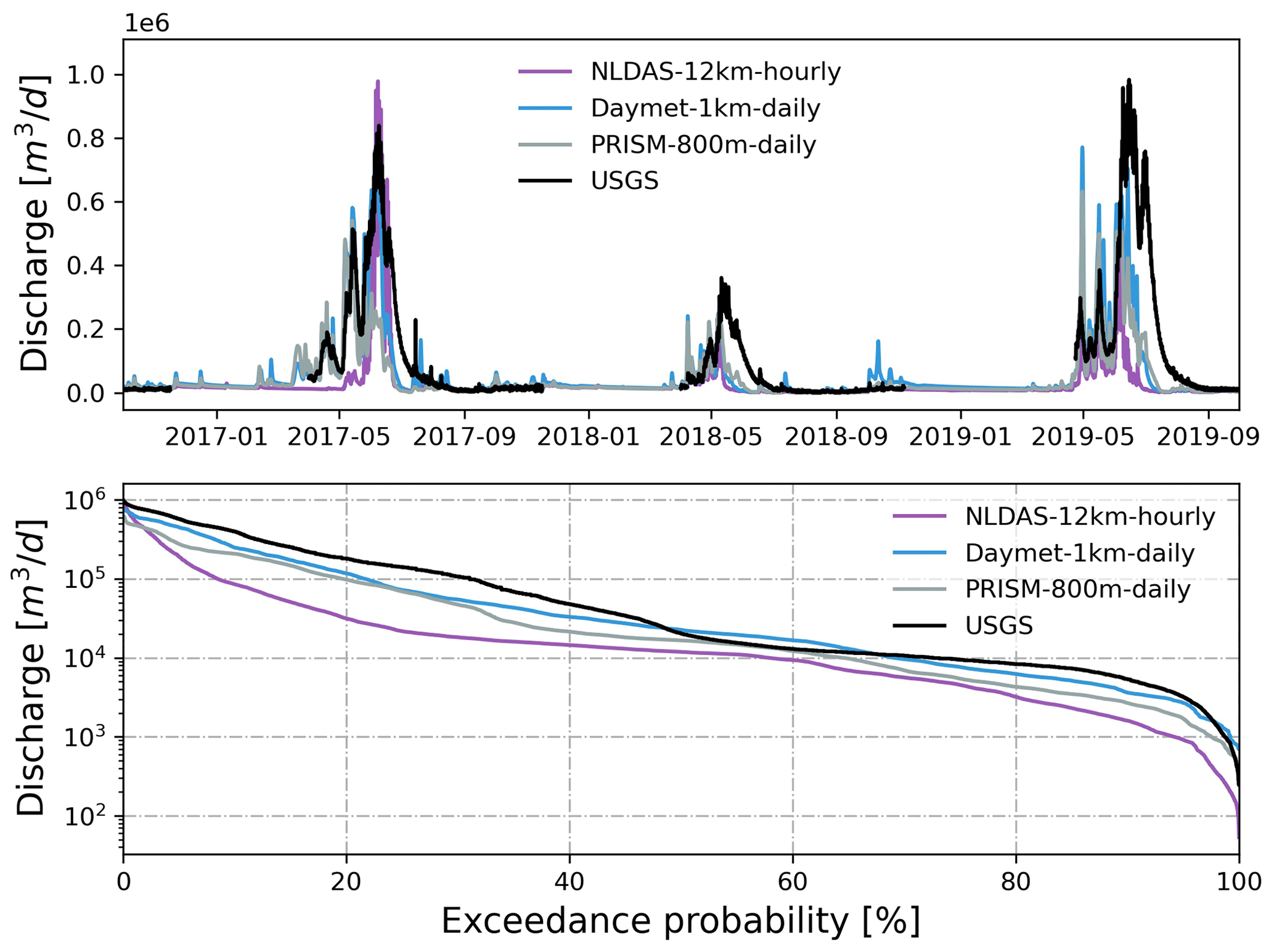
Figure 4 Simulated hourly discharge at the watershed outlet compared to USGS hourly streamflow forced by different precipitation and temperatures from each GMF. Also shown is the flow duration curve comparison.

Triple collocation analysis (TCA) was performed for precipitation and temperature using three GMFs over the East Taylor Watershed (see details in Appendix A2). Both precipitation and temperature showed strong spatial heterogeneity of the noise standard error in all three GMFs. On average, Daymet and PRISM showed less error compared to NLDAS for both precipitation and temperature, though the temperature errors in some locations of Daymet were higher than those of PRISM and NLDAS.

3.2 ATS simulations driven by different meteorological forcing products

To compare the effects of different GMF products on the ATS simulations, precipitation and temperature from each GMF were used as the primary forcing variables with the same other variables (e.g., solar radiation, humidity) from Daymet. To further isolate the impact of different meteorological forcing variables, precipitation and temperature from each GMF were systematically varied. For example, different precipitation from each GMF were used while keeping temperature the same in each simulation, and vice versa.

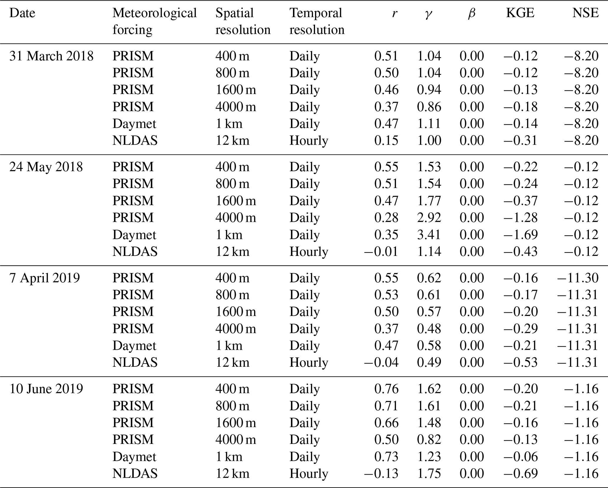
Using different precipitation and temperatures, simulated hourly streamflow forced by Daymet (1 km, daily) showed better performance against USGS hourly streamflow, followed by PRISM (800 m, daily) and NLDAS (12 km, hourly) during a 3-year simulation period (Fig. 4). At their native resolutions, Daymet outperformed PRISM and NLDAS with the largest KGE (0.62) and NSE (0.54) against observed streamflow (also see the statistical summary in Table 2). The high agreement between observed and simulated streamflow forced by Daymet is remarkable given that the ATS model has not been calibrated. In general, all three models underestimated discharge (β<1) while showing slightly more variability (γ>1), especially in 2018 and 2019. As expected, models using hourly NLDAS showed larger variability (γ=1.54) due to the highly dynamic flow variations in simulated streamflow compared to those using daily Daymet or PRISM. Daymet underestimated peak flows, but it showed larger flow variability during low flows and early spring.

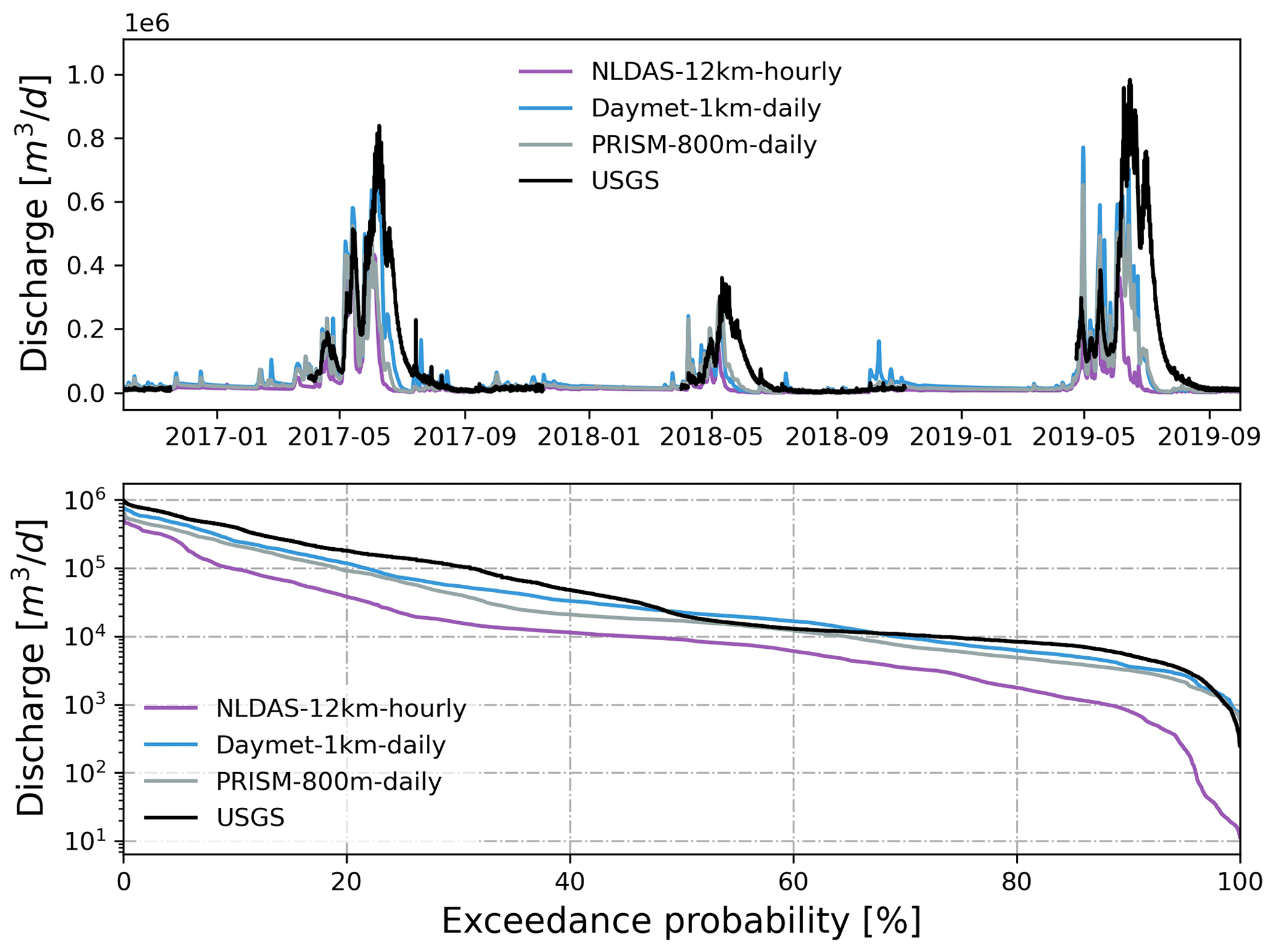
Figure 5 Simulated hourly discharge at the watershed outlet compared to USGS hourly streamflow forced by different precipitation from each GMF. Also shown is the flow duration curve comparison.

Table 2 Summary of statistical metrics for evaluation of streamflow at the watershed outlet using precipitation and/or temperature from different meteorological forcings.

Not surprisingly, precipitation played a more important role than temperature in driving the simulated watershed responses. Using different precipitation sources alone had similar performance compared to using both precipitation and temperature from each GMF. In both cases, Daymet outperformed PRISM and NLDAS in simulated streamflow (Fig. 5). The KGE and NSE metrics from Daymet and PRISM were much higher than those from NLDAS (Table 2). However, using different temperature sources alone had little effect on the simulated streamflow (Fig. 6). Both KGE and NSE metrics were very similar among different GMFs (Table 2).

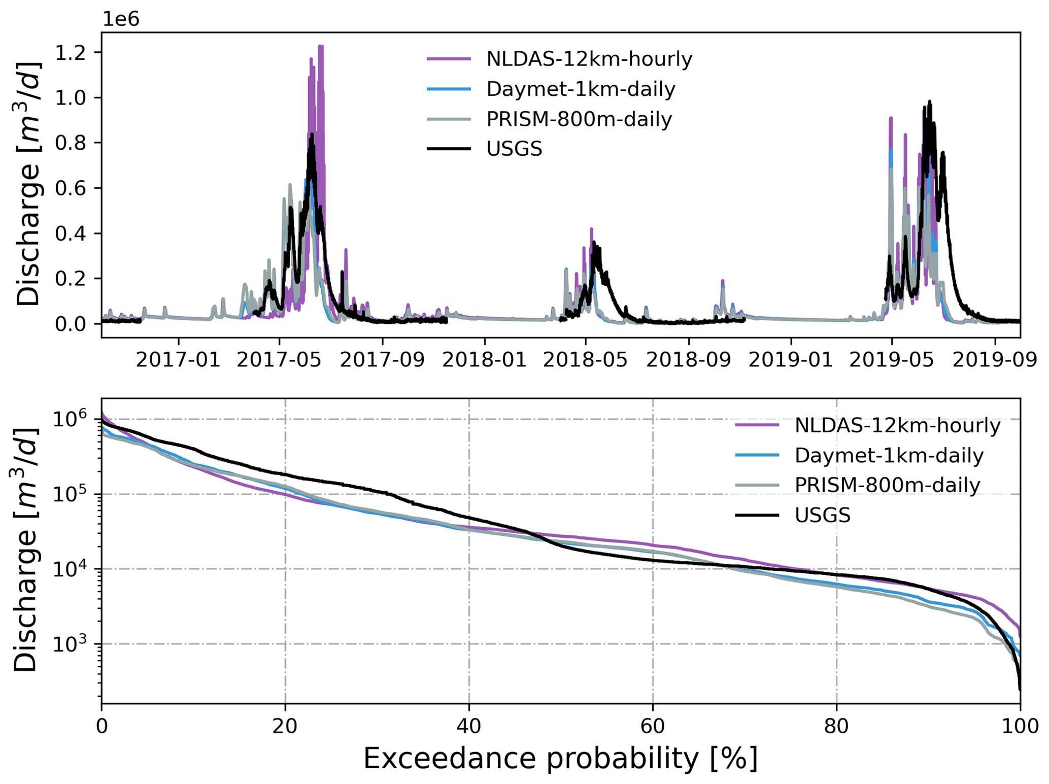
Figure 6 Simulated hourly discharge at the watershed outlet compared to USGS hourly streamflow forced by different temperatures from each GMF. Also shown is the flow duration curve comparison.

Average SWE across the watershed showed large differences between different meteorological forcings (Fig. 7). Daymet had the largest simulated SWE on average, while NLDAS had the smallest simulated SWE. PRISM produced a similar SWE pattern with Daymet, and their magnitude was very close except for the year 2017. The accumulation of snow started around the same time for all three meteorological forcings, though snow disappeared early for NLDAS in the last 2 years.

Spatially, all meteorological forcings significantly underestimated SWE (β≈0) when compared to SWE from ASO (Table 4), and the difference becomes larger at higher elevation with more accumulated snow (Fig. 9). The large difference may be attributed to the higher spatial resolution (50 m) used in the ASO snow survey than the spatial resolution of the GMF. Simulated SWE by the three models showed a larger variability (γ>1) than the observed SWE, except on 7 April 2019, when variability was smaller than the observed SWE. Interestingly, the largest variability occurred on 24 May 2018 when little snow was accumulated on the surface. Most of the time, PRISM showed a higher correlation between simulated and observed SWE than that from Daymet and NLDAS. In contrast, NLDAS showed the poorest correlation (r<0.2) with observation.

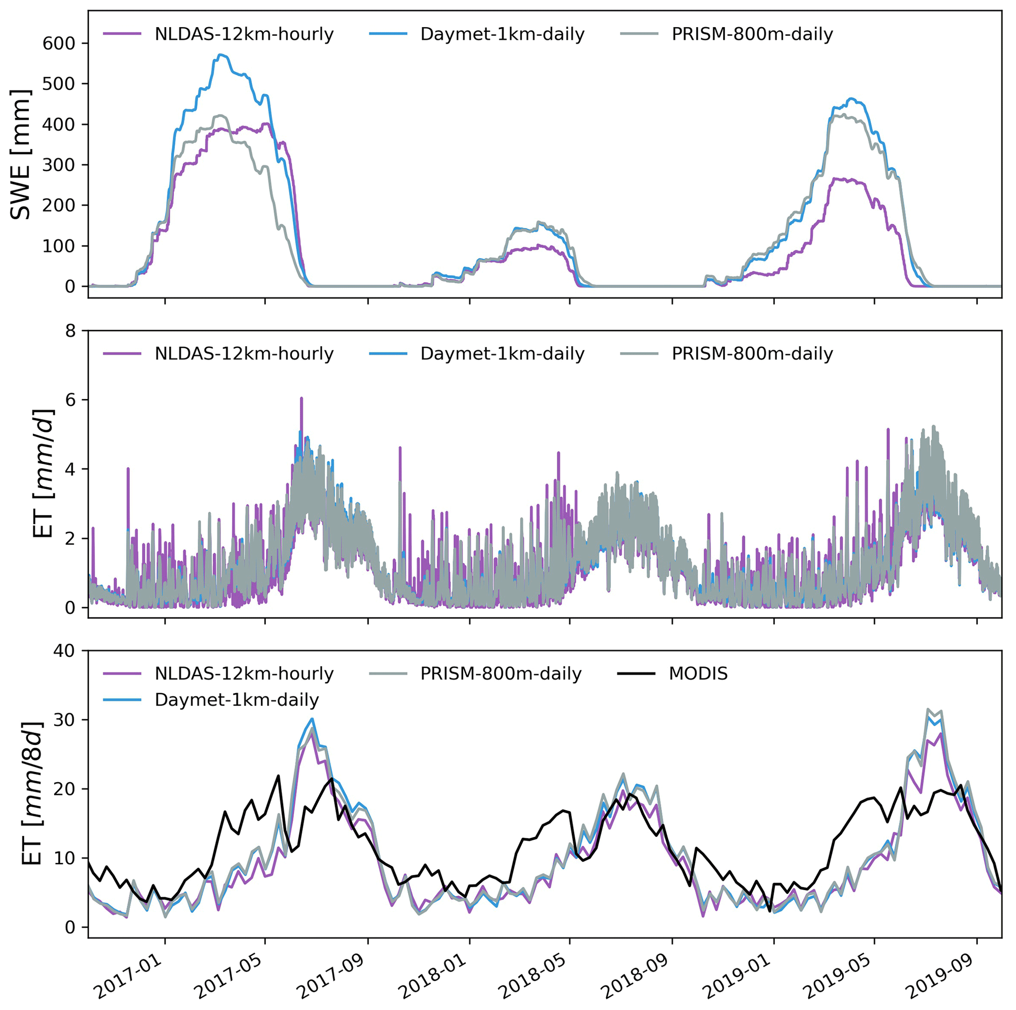
Figure 7 Simulated hourly watershed average SWE and ET under different meteorological forcings. Also shown is the comparison between MODIS and simulated 8 d composite ET.

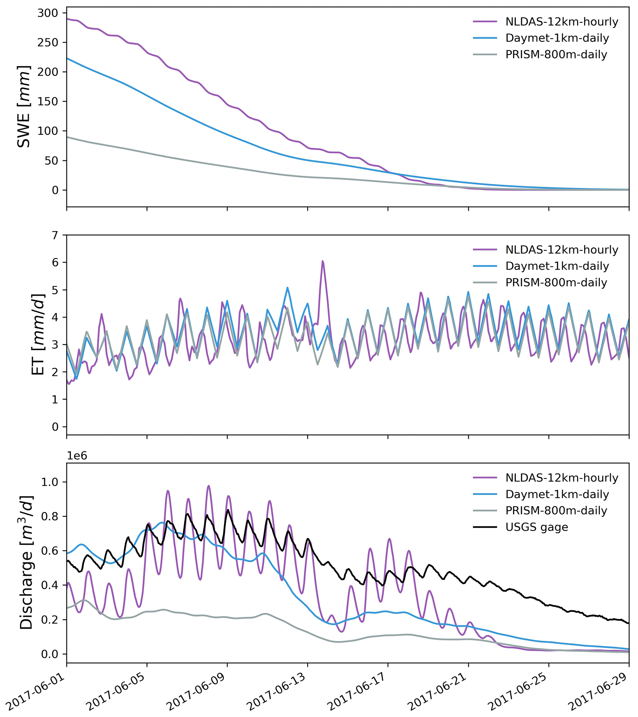
Figure 8 Zoomed-in plot showing simulated hourly watershed average SWE, ET, and discharge under different meteorological forcings from 1 to 29 June 2017.

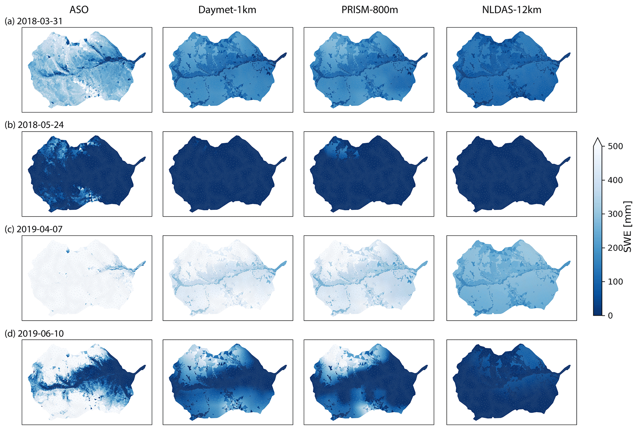
Figure 9 Spatial distribution of SWE under different meteorological forcings and their comparison with ASO SWE data at four different survey times.

All three GMFs showed similar ET dynamics because they used the same solar radiation from Daymet (Figs. 7 and 8). Compared to the remote-sensed 8 d composite ET from MODIS, all three meteorological forcings showed a consistent seasonal trend with MODIS, with underestimated ET in the spring. Additionally, the simulated 8 d composite ET by Daymet and PRISM was higher than that from NLDAS in the peak growing season in 2017 and 2019.

3.3 Effects of meteorological forcing spatial resolution

To evaluate the effects of spatial resolution of meteorological forcing, precipitation and temperature from different spatial resolutions of PRISM and Daymet were used to drive the model. Because the findings from both PRISM and Daymet were similar, only results from PRISM were summarized below (see Appendix A3 for Daymet comparison in Figs. A3 and A4). As the spatial resolution became finer, the spatial pattern of precipitation and temperature became more heterogeneous and was more strongly associated with local topography, land use, and land cover. By contrast, coarser-resolution meteorological forcing produced more homogeneous and smoother spatial patterns with less accuracy (Figs. A8 and A9). In addition to precipitation and temperature, the effect of spatial resolution of solar radiation (i.e., S_rad) was tested and was found to have little impact on watershed hydrologic variables (see Appendix A4).

The simulated discharge showed similar performance in terms of KGE and NSE compared to the observation when meteorological forcing spatial resolution was ≤1600 m (Table 2). In fact, the KGE and NSE of 400, 800, and 1600 m resolution were almost identical. All four resolutions showed higher variability (γ>1) with relatively high correlation (r>0.6) in simulated streamflow than the observation. The variability became larger (γ=1.20) and the correlation became weaker (r=0.64) as meteorological forcing spatial resolution reached 4 km (Fig. 10). The simulated SWE and total water storage changes were almost identical for all spatial resolutions except during the snowmelt period, when the 4 km spatial resolution showed faster snowmelt in early summer across all 3 years (Fig. A10). The spatial distribution of SWE when compared to ASO SWE showed a significantly large bias (β≈0) and thus negative KGE and NSE for all spatial resolution at all times (Fig. 11 and Table 4). Generally, the 4 km resolution had the worst performance and became most obvious on 24 May 2018. PRISM at 400 and 800 m resolution showed a similar spatial pattern and thus a similar correlation with ASO SWE.

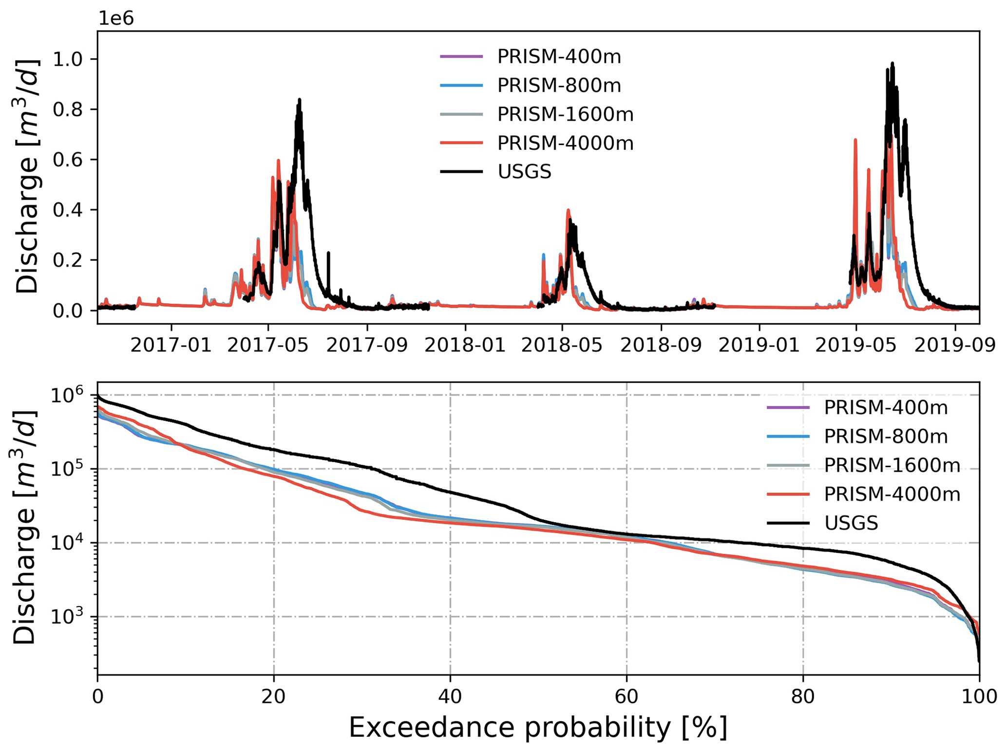
Figure 10 Simulated discharge at the watershed outlet compared to the USGS gage under different spatial resolutions of PRISM. Also shown is the flow duration curve comparison.

Figure 11 Spatial distribution of SWE under different spatial resolutions of PRISM and their comparison with ASO SWE data at four different survey times.

Soil moisture at the top 5 cm layer showed a similar pattern when spatial resolution was ≤1600 m (Fig. A11). The differences between 4 km resolution and finer resolution became obvious during the snowmelt period (24 May 2018 and 10 June 2019), when soil becomes saturated. For example, soil in the northwestern region from the 4 km resolution was wetter on 24 May 2018, whereas soil close to the outlet from the 4 km resolution was wetter on 10 June 2019. Similarly, spatially distributed ET did not show a significant difference until meteorological forcing resolution reached 4 km (Fig. A12).

Surface ponded depth showed very little difference between different spatial resolutions. Four locations (labeled as 1–4 in Fig. 1) were selected across the watershed to show the ponded depth variations (Fig. 12). One was located at the upstream branch, and the other three were located along the Coal Creek main stem. Similarly to the watershed discharge, ponded depth only differed when the spatial resolution was coarsened to 4 km. The 4 km resolution had a faster recession during peak flows compared to results from other finer resolutions, and the 4 km resolution was also less responsive to rainfall. On average, surface ponded depth varied less than 0.2 m during peak flows.

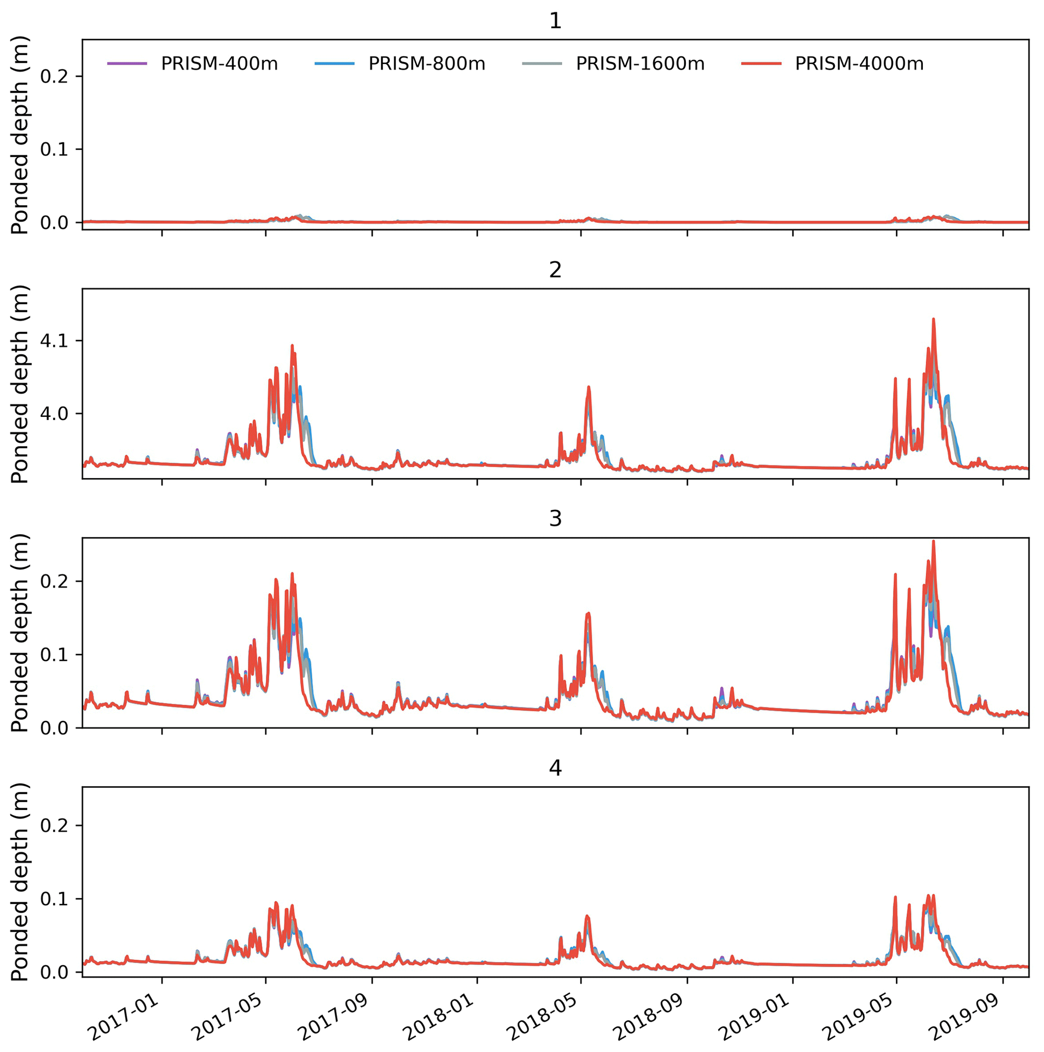
Figure 12 Simulated surface ponded depth at four selected locations under different spatial resolutions of PRISM.

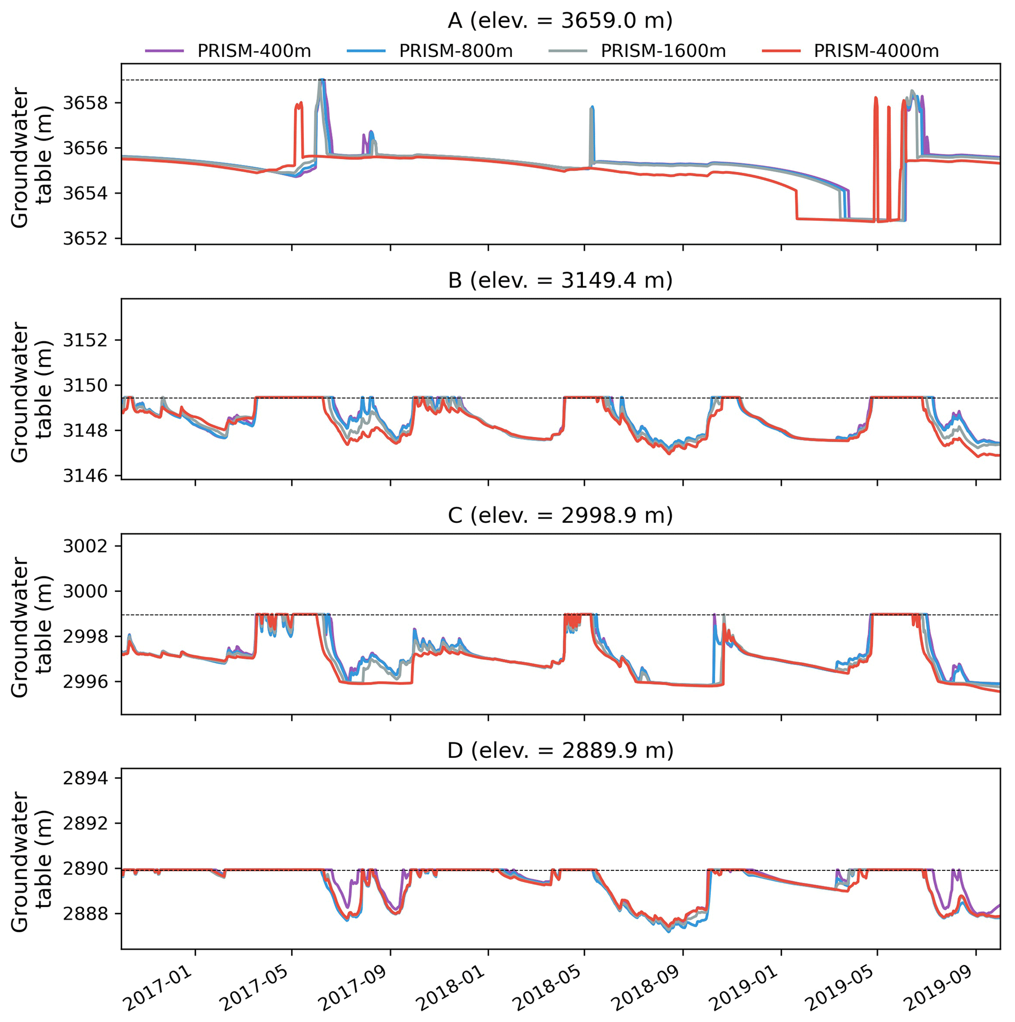
A transect was selected running from mountain top to river valley bottom with four selected observation locations (labeled as A–D in Fig. 1), and groundwater table time series was plotted in Fig. 13. In general, groundwater rose during snowmelt (April to June) and rainfall events and fell in the dry period (July to September). Location A was at the mountain top, and the groundwater table was ∼4 m below the land surface except during the snowmelt period, when the groundwater table rose to the surface. Since location A was dominated by snow and receives less rainfall, the rise in the groundwater table was mainly due to snowmelt. Locations B and C showed similar trends in groundwater table fluctuations; however, they showed more peaks since they were influenced by both snowmelt and rainfall. The groundwater table at location D was mostly close to the surface except during the dry season, when groundwater started to decline. The 4 km resolution behaved very differently from the other finer resolutions at location A, where the groundwater table peaked earlier due to earlier infiltration from snow. In a dry year in 2018, the groundwater table did not even rise during the snowmelt period at location A. In general, the coarser the meteorological forcing resolution, the larger the bias in precipitation and the more the groundwater table buffered from snowmelt and rainfall.

Figure 13 Simulated groundwater table at four selected locations (A–D) under different spatial resolutions of PRISM. Dashed line indicates the surface elevation. Also, see Fig. 1 for location detail.

3.4 Effects of meteorological forcing temporal resolution

The effect of meteorological forcing (i.e., precipitation and temperature) temporal resolution on watershed hydrologic simulations was evaluated by using hourly, 12-hourly, and daily PRISM datasets. All resolutions outputted hydrological variables in an hourly timestep and were compared to hourly observed streamflow. In addition to precipitation and temperature, the effect of temporal resolution of solar radiation (i.e., S_rad) was tested. The temporal resolution of solar radiation slightly changed the dynamics of streamflow, but overall the impact on watershed hydrologic variables was negligible (see Appendix A4).

The match between simulated and observed hourly discharge in terms of KGE was better with daily resolution than hourly and 12-hourly temporal resolution (see Fig. 14 and Table 3). The low performance (KGE=0.20) under hourly resolution was mainly due to the relatively lower correlation (r=0.43) and higher variability (γ=1.12) between simulated and observed streamflow. This is not surprising since hourly meteorological forcing has a more dynamic forcing pattern including hourly temperature and precipitation, and thus it yielded a more dynamic overland flow pattern that can be quite different from field observations. To investigate the hydrograph in more detail, discharge time series were zoomed into the high-flow season in 2017 (Fig. 15). It was clear that models driven by hourly and 12-hourly PRISM contained sub-daily flow fluctuations that would be absent in models driven by the daily PRISM. Models driven by 12-hourly PRISM had a weaker diurnal flow pattern in terms of magnitude. This is because hourly PRISM retains the diurnal signal of air temperature and thus the diurnal snowmelt pattern, whereas 12-hourly PRISM had a weaker diurnal signal due to only changing air temperature every 12 h (Fig. 15). On the other hand, daily PRISM assumes uniform air temperature throughout a day and thus produced streamflow that was much smoother without diurnal fluctuations. In general, discharge from the hourly PRISM peaked earlier and had a less steep recession limb compared to that from 12-hourly and daily PRISM.

Table 3 Summary of statistical metrics for evaluation of streamflow at the watershed outlet under different meteorological forcing spatial and temporal resolutions.

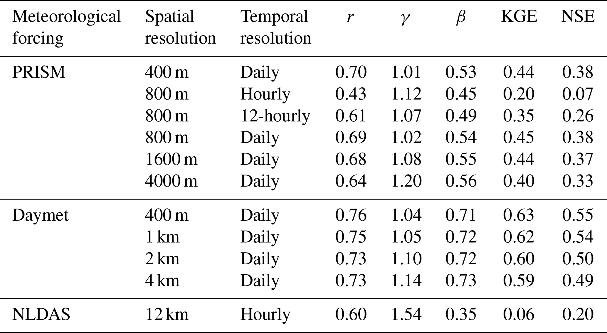
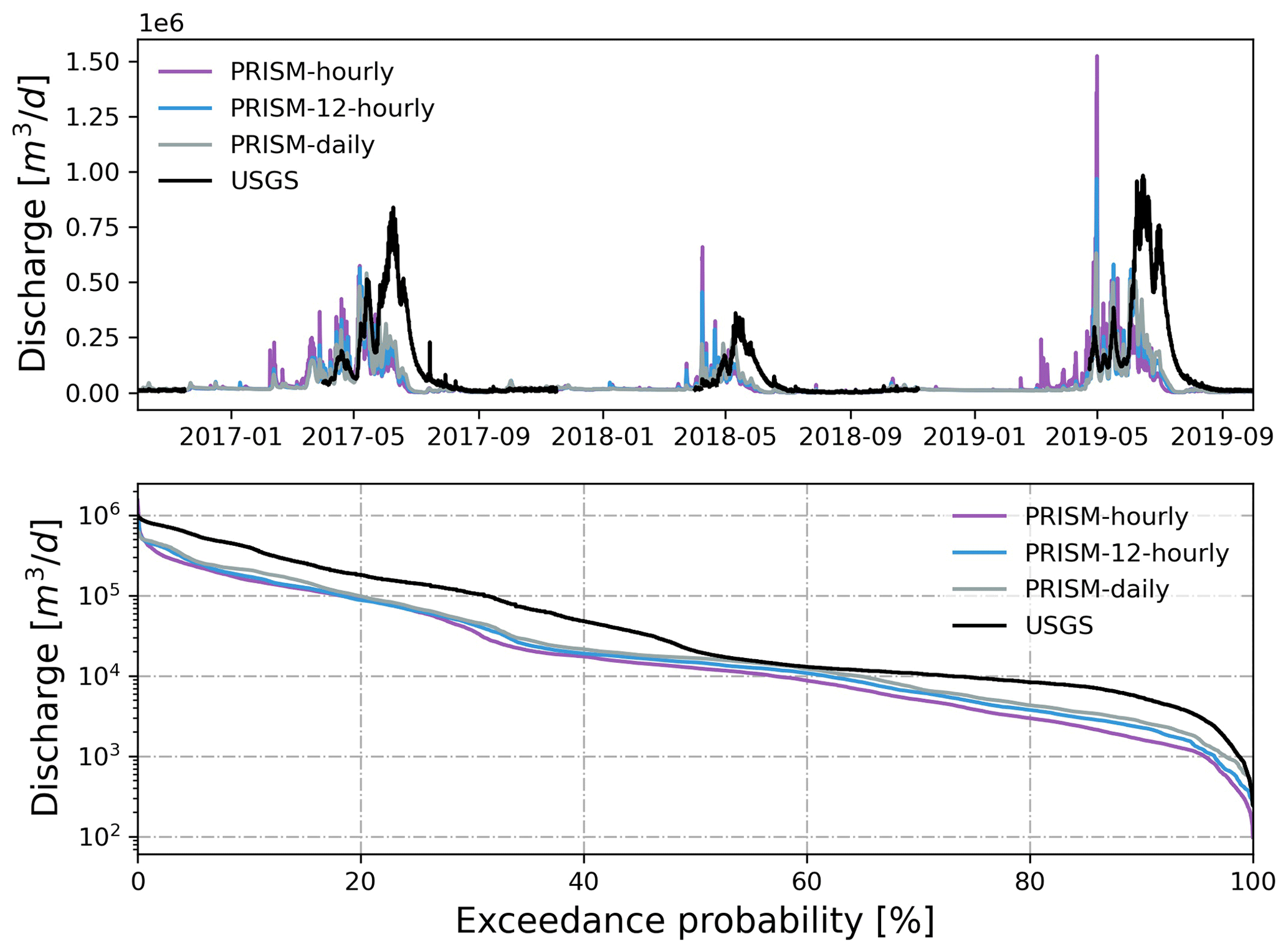
Figure 14 Simulated hourly discharge at the watershed outlet compared to hourly USGS streamflow under different temporal resolutions of PRISM. Also shown is the flow duration curve comparison.

Figure 15 Zoomed-in plots showing hourly simulated snowmelt, ET, and discharge under different temporal resolutions of PRISM in May 2017.

Hourly PRISM had the largest snowmelt and ET variations, followed by 12-hourly and daily PRISM (Fig. 15). Compared to the remote-sensed 8 d composite ET from MODIS, the simulated 8 d composite ET forced by the different temporal resolution of PRISM showed a consistent seasonal trend with MODIS (Fig. 16). However, significant model underestimation was observed in the spring. All three PRISM resolutions showed similar trends of seasonal snowpack accumulation. However, there was a large difference in peak SWE. Hourly PRISM reached a smaller SWE peak, and the snow melted earlier compared to 12-hourly and daily PRISM, which might be the combined effects of faster snowmelt and slightly larger ET.

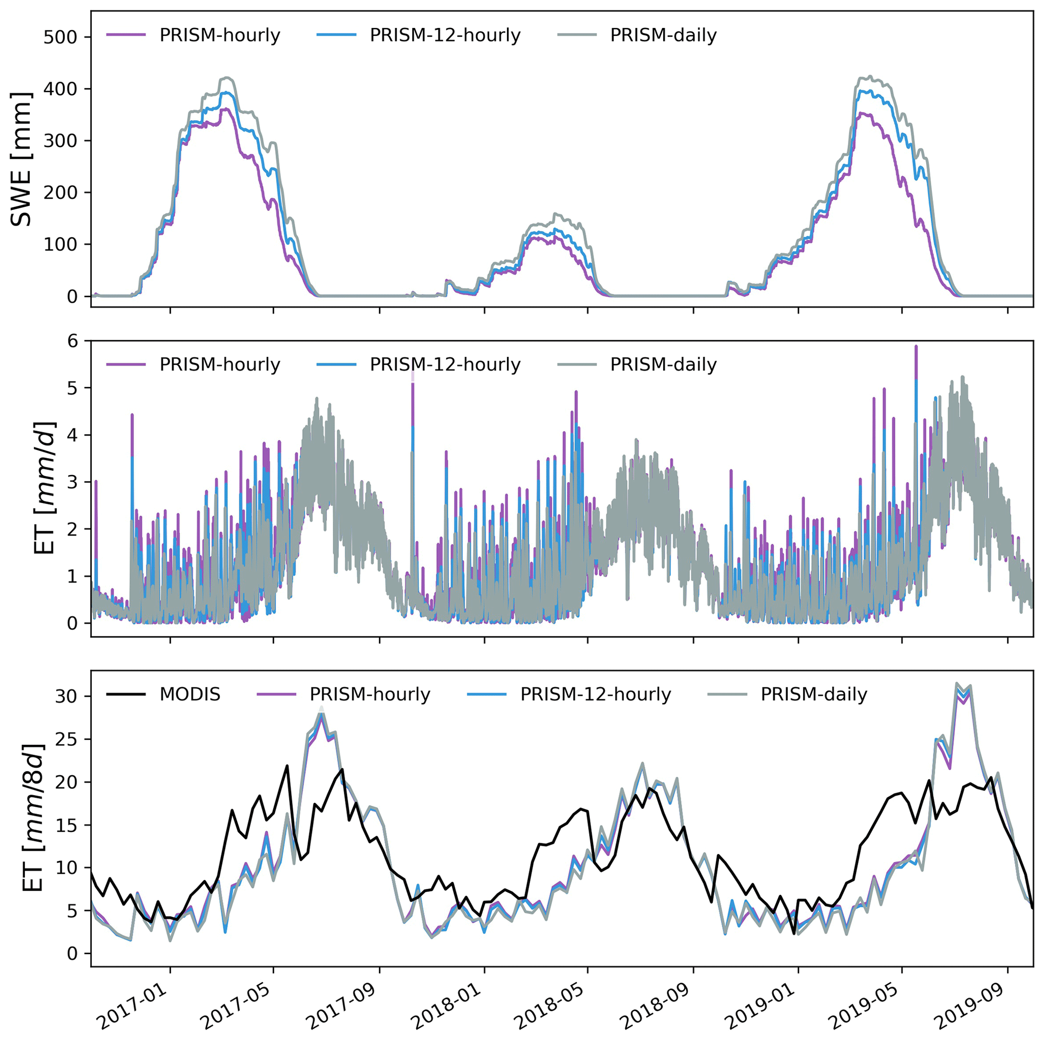
Figure 16 Simulated watershed average SWE and ET under different temporal resolutions of PRISM. Also shown is the comparison between MODIS and simulated 8 d composite ET.

4 Discussions

4.1 The choice of gridded meteorological forcing for integrated watershed simulation

We compared three GMFs at their native resolution, Daymet (daily, 1 km), PRISM (daily, 800 m), and NLDAS (hourly, ∼12 km), in driving watershed responses including watershed outlet discharge and spatially distributed variables such as SWE and ET. Can we choose the “best” meteorological forcing for integrated watershed modeling based on discharge comparison alone? What are the strengths and weaknesses of each GMF?

In surface hydrologic modeling, hydrologists often judge the performance of a numerical model by the ability to match the streamflow at the watershed outlet (Staudinger et al., 2019). However, streamflow alone is not good enough to evaluate the performance in meteorological forcing because discharge at the watershed outlet has limited information on the spatial distribution of model outputs (e.g., SWE). Even though simulated streamflow from Daymet has the best match (i.e., highest KGE) against observation, the spatially distributed SWE from Daymet has a weaker correlation with the observed SWE from the ASO survey than that from PRISM. Both Daymet and PRISM perform better than NLDAS in simulating discharge and spatial SWE due to their relatively fine spatial resolution. As shown in Fig. 9, NLDAS hardly captures the spatial heterogeneity of SWE when compared to ASO SWE. The entire watershed area (∼53.2 km²) is smaller than the size of 1 pixel of the NLDAS grid ($\sim \mathrm{12}\times \mathrm{12}$ km or ∼144 km²), making the meteorological forcing almost homogeneous at the watershed scale.

For a watershed simulation that usually has a mesh resolution < 1 km, Daymet or PRISM provides the best spatial resolution available across the CONUS. However, they do not have the complete forcing dataset that could be directly applied to watershed models without filling in the missing dataset. Daymet has most of the forcing variables except wind speed and longwave radiation. PRISM is missing both wind speed and solar radiation (both shortwave and longwave radiation), which is important for calculating surface energy balance and estimating ET. A common approach is to fill in the missing variables using a different source. For example, Mourtzinis et al. (2017) used solar radiation from the National Aeronautics and Space Administration’s POWER (NASA-POWER) database (12 000 km² resolution) combined with PRISM's temperature and precipitation to simulate a crop model. In our study, we used Daymet as a source of solar radiation for PRISM, and the model was able to simulate streamflow reasonably well (KGE=0.45) (Table 2) while capturing the spatial heterogeneity of distributed variables.

On the other hand, NLDAS provides the most complete forcing dataset with hourly resolution but comes with a spatial resolution of ∼12 km, which is too coarse for watershed simulation, especially watersheds with complex terrain. The spatial resolution may become less important as model resolution becomes coarser, and the focus is on the system-scale water budget. For example, NLDAS at its native resolution has been applied at the continental scale to study transpiration partitioning using ParFlow-CLM at 1 km resolution (Maxwell and Condon, 2016). Past studies have also attempted downscaling of NLDAS to much finer spatial resolution (Ko et al., 2019; Pan et al., 2016). For example, Ko et al. (2019) downscaled the meteorological forcing variables from the 12 km resolution of NLDAS to 1 km resolution using high-resolution terrain information at the Río Sonora basin. There have been other attempts to merge the high spatial resolution of the PRISM dataset with the NLDAS dataset, which produced a complete forcing dataset of daily, 4 km resolution covering the CONUS (Abatzoglou, 2013).

Ideally, the GMF with a finer spatiotemporal resolution while providing the most complete forcing is desirable. However, none of the three GMFs is perfect. An alternative approach is to use meteorological forcing outputted from climate models such as WRF. It has the flexibility of generating much finer spatial and temporal resolution output while providing all available meteorological forcings. Maina et al. (2020) used the nested-domain configuration of WRF to dynamically generate meteorological forcing variables at various spatial resolutions (from 0.5 to 13.5 km) for use with ParFlow-CLM. Although forcing generated by WRF provides a viable option for meteorological input in the hydrologic model, it requires additional expertise and effort to set up and run the WRF model, which is more challenging than directly using the publicly available gridded forcing (e.g., Daymet).

Table 4 Summary of statistical metrics used for evaluation of spatially distributed SWE under different meteorological forcings at different times compared to observed SWE from ASO.

4.2 Spatial vs. temporal resolution: which one is more important?

Is there an optimal spatiotemporal resolution of meteorological forcing for driving watershed simulation while producing realistic results? Should we choose finer spatial resolution over finer temporal resolution? Depending on the quantity of interest and the spatial and temporal scale of the study, the choice may differ. In this study, watershed outlet discharge is shown to be less sensitive to both the spatial and temporal resolution of meteorological forcing because it is an accumulative quantity. The simulated discharge is almost identical between PRISM 400, 800, and 1600 m resolution. The simulated discharge only becomes noticeably worse when the spatial resolution of meteorological forcing is coarsened to 4000 m (or 30 % of the watershed area). Similarly, the watershed average SWE, ET, and total water storage do not show significant differences between different spatial resolutions of PRISM.

The spatial resolution becomes more important if the quantity of interests is the spatially distributed hydrologic variables. For example, the SWE distribution under 400 and 800 m PRISM resembles more closely the ASO SWE than results under much coarser spatial resolution. Maina et al. (2020) also found the SWE distribution to be sensitive to the spatial resolution of meteorological forcing, with the finer resolution being able to accurately reproduce SWE spatial distribution as well as total SWE volume. In addition, a higher spatial resolution of forcing would preserve the spatial heterogeneity of distributed variables better and may provide better estimates of variables at point locations (e.g., SWE at the NRCS's Snowpack Telemetry (SNOTEL) stations and groundwater table at wells). For example, the groundwater table at high elevations can be quite different under different spatial resolutions of meteorological forcing (Fig. 13).

Temporal resolution becomes more important than spatial resolution when simulating storm events or flash floods that happen within several hours, resulting in a sharp increase in stream discharge (Ochoa-Rodriguez et al., 2015). The regular, periodic streamflow fluctuations induced by sub-daily snowmelt or ET could also impact the hyporheic exchange between surface water and groundwater (Loheide and Lundquist, 2009), which in turn impacts nutrient cycling in the stream and hyporheic zone biogeochemical processes (Shuai et al., 2017; Song et al., 2018). By contrast, it is challenging to match the simulated variable from high temporal resolution with field observation. For example, the performance in simulated discharge deteriorates when temporal resolution increases from daily to hourly using PRISM (Fig. 14). Additionally, hourly meteorological forcing is difficult to obtain and may be subject to large bias and errors. There are also sparse weather stations that collect hourly or higher-frequency data. Thus it is impossible to obtain sub-daily resolution by direct interpolation across weather stations. The current available hourly meteorological forcing is usually disaggregated from coarse temporal resolution. For example, the hourly NLDAS is disaggregated from NARR 3-hourly frequency. Previous studies have shown that NLDAS had large discrepancies towards SWE at higher elevation where lower SWE was simulated (Sheffield et al., 2003; Maxwell and Condon, 2016). Air temperature has also been shown to be systematically colder in winter and warmer in the spring months compared to the observations (Pan et al., 2003). These biases could be attributed to the ∼12 km spatial resolution that greatly smoothed the local topographic variability.

4.3 Limitations, implications, and transferability of the current study

There is a lack of high-resolution observation data to compare to the simulated variables. For example, the snow survey from ASO has only been conducted a total of four times at this watershed and misses the temporal dynamics of snow depth. There is also no single SNOTEL station within the watershed that we can use to compare simulated SWE at a point location with the observed SWE. In addition to snow, we also do not have high-resolution ET data. Although MODIS provides an 8 d composite ET, it is relatively coarse compared to the temporal resolution examined in the study. In the subsurface, there are no observed groundwater table depth or soil moisture data that can be used for the comparison. The remote-sensed soil moisture product (9 to 36 km resolution) from Soil Moisture Active Passive (SMAP) is likely to be too coarse to have any meaningful comparison.

Uncertainty in the meteorological forcing has not been quantified. There is undoubtedly uncertainty in each GMF that may impact the simulated watershed responses; however, this is not the focus of this study. Precipitation collected from ground-based gages often has measurement uncertainty that could lead to large uncertainty in interpolated gridded datasets, especially in the mountainous region where the gage network is sparse (Schreiner‐McGraw and Ajami, 2020). In general, PRISM is assumed to perform better in matching gage observation in the mountainous regions compared to Daymet because of the relatively complex interpolation method (Daly et al., 2008). However, PRISM does not outperform Daymet in all gages (see Fig. 3). Further, in areas where the terrain is flat and the gage network is dense, Daymet might perform better than, if not equally well as, PRISM. Therefore, it is important to put the results into context when comparing different meteorological forcings in a watershed setting.

Uncertainty in model parameterization has not been investigated; however, it does not change the conclusions of this study, as all simulations use the same set of model parameters except for meteorological forcing. It is well known that model parameters such as subsurface structure and properties impact surface and subsurface flows and consequently ET and water storage. As shown in this study, models using different meteorological forcings may produce dramatically different watershed responses including streamflow. This has important implications for model calibration, where the objective is to minimize the differences between simulated and observed streamflow, which is true for most watershed hydrologic model calibration studies (Cromwell et al., 2021). The choice of GMF affects the simulated streamflow and in turn the optimal parameters that are calibrated using the simulated streamflow. Elsner et al. (2014) showed that there were substantial differences in calibrated model parameters and simulated water balance using four different meteorological forcings for the same watershed. As a result, the choice of meteorological forcing plays a critical role in model calibration and thus long-term planning and watershed management using such a calibrated model. Studying the impact of different meteorological forcings on model calibration is the focus of our future work.

In this study, we choose Coal Creek as an illustrative example to show the effects of meteorological forcing spatiotemporal resolution on watershed simulations. The study site has strong variations in topography and land cover, which is an ideal site for testing heterogeneous spatial–temporal pattern of meteorological forcing. Our conclusions would hold for other mountainous headwater watersheds that are dominated by snow because we did not make any site-specific assumptions. However, additional studies are needed to evaluate the GMF in other areas that are not dominated by snow.

5 Conclusions

This study aimed to compare three widely available GMFs (i.e., Daymet, PRISM and NLDAS) and evaluate the impacts of spatiotemporal resolution of meteorological forcing on simulated streamflow, ET, SWE, soil moisture, surface ponded depth and groundwater table in a snow-dominated mountainous watershed. The different spatial and temporal resolutions were generated by either downscaling or upscaling the native meteorological forcing resolution. The resulting meteorological forcing was then applied as input to drive a fully distributed, integrated watershed model (i.e., ATS).

To evaluate the performance of meteorological forcing, one should compare all aspects of watershed hydrologic responses. Daymet has the best match in simulated streamflow; however, the simulated spatially distributed SWE has a weaker correlation with the observed ASO SWE compared to that from PRISM. NLDAS performs worst in both simulated streamflow and spatially distributed SWE due to its coarsest grid resolution. By systematically varying precipitation and temperature from each GMF, streamflow is found to be more sensitive to precipitation than temperature. Overall, NLDAS provides the most comprehensive dataset with the highest temporal resolution (hourly) but comes with a spatial resolution of ∼12 km that is too coarse for watershed simulation, especially areas with complex terrain. By contrast, both PRISM (800 m) and Daymet (1 km) provide finer spatial resolution, capable of simulating watershed hydrological variables at high resolution, though PRISM is missing the important solar radiation. Using precipitation and temperature from PRISM along with solar radiation from Daymet provides an alternative to driving watershed simulation with relatively high accuracy.

Using different spatial resolutions of PRISM ranging from 400 m to 4 km, the simulated discharge shows a minor difference when spatial resolution is <4 km (or the grid area is $<\sim \mathrm{30}$ % of the watershed area). Similarly, the watershed average SWE, ET, and total water storage do not show significant differences between different spatial resolutions. Spatial resolution becomes more important when simulating spatially distributed hydrologic variables such as SWE and groundwater table.

Using a different temporal resolution of PRISM (hourly to daily), the simulated discharge showed better performance with daily resolution compared to that forced by 12-hourly and hourly resolution. However, models forced by the sub-daily resolution preserve the dynamic watershed responses (e.g., diurnal fluctuation of streamflow) that are absent in results forced by daily resolution. This may have important implications for watershed biogeochemical reactions that often happen at sub-daily timescales.

It is difficult to choose the “best” meteorological forcing dataset because each dataset has its strengths and weaknesses, and what is best depends on the quantity of interest and its spatial and temporal scale. Ideally, the GMF with a finer spatiotemporal resolution while providing the most complete forcing is desirable. An alternative approach is to use meteorological forcing outputted from climate models such as WRF, which has the flexibility of generating much finer spatial and temporal resolution output while providing all available meteorological forcing datasets.

The choice of GMF affects the simulated streamflow and thus has an important implication for model calibration when the objective is to minimize the differences between simulated and observed streamflow. The findings of the effects of meteorological forcing spatiotemporal resolution on watershed simulations could be transferable to other mountainous watersheds that are snow-dominated.

Appendix A

A1 Calendar day definition used in the meteorological datasets

Table A1 Calendar day as defined in meteorological datasets and USGS gage.

Abbreviations: D⁻¹: previous day; D: current day; D⁺¹: next day.

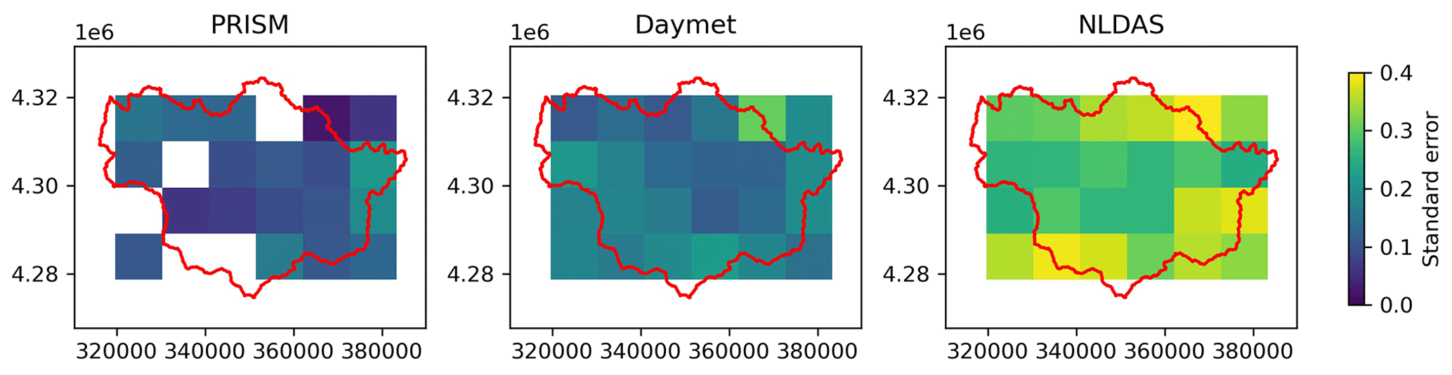
Figure A1 TCA results for precipitation data in the three GMFs. The color map shows the standard error (the lower the better) for each pixel region.

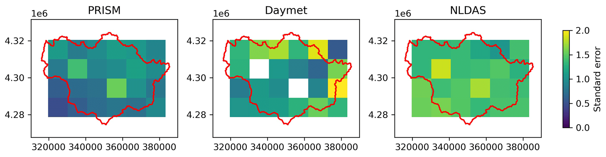
Figure A2 TCA results for temperature data in the three GMFs. The color map shows the standard error (the lower the better) for each pixel region.

A2 Triple collocation analysis (TCA) of meteorological forcing

TCA was used to characterize the uncertainties (e.g., error variance and signal-to-noise ratio) in each of the GMFs without knowing the ground truth. Here, we applied TCA to the precipitation and temperature product, respectively, using the three GMFs over the larger East Taylor watershed. The PRISM and Daymet products have been upscaled to a 12 km grid to be consistent with the spatial resolution of the NLDAS product. The aggregated daily NLDAS was used to be consistent with the temporal resolution of PRISM and Daymet. The major assumption for the TCA is that the error models are linear and independent between different sources, which is not appropriate for precipitation data (Kratzert et al., 2021). Instead, we chose a multiplicative error model for the precipitation source following the methodology of Alemohammad et al. (2015). Because log-transformed precipitation values were used in the multiplicative model, the daily precipitation was temporally aggregated to weekly values to avoid zero precipitation values. As a result, the total number of sample sizes across the temporal domain was significantly reduced, which could pose a challenge for the TCA when the sample size was small. The missing values in Figs. A1 and A2 (white pixels) were the result of having too few samples.

A3 Comparison of model outputs from different spatial resolutions of Daymet

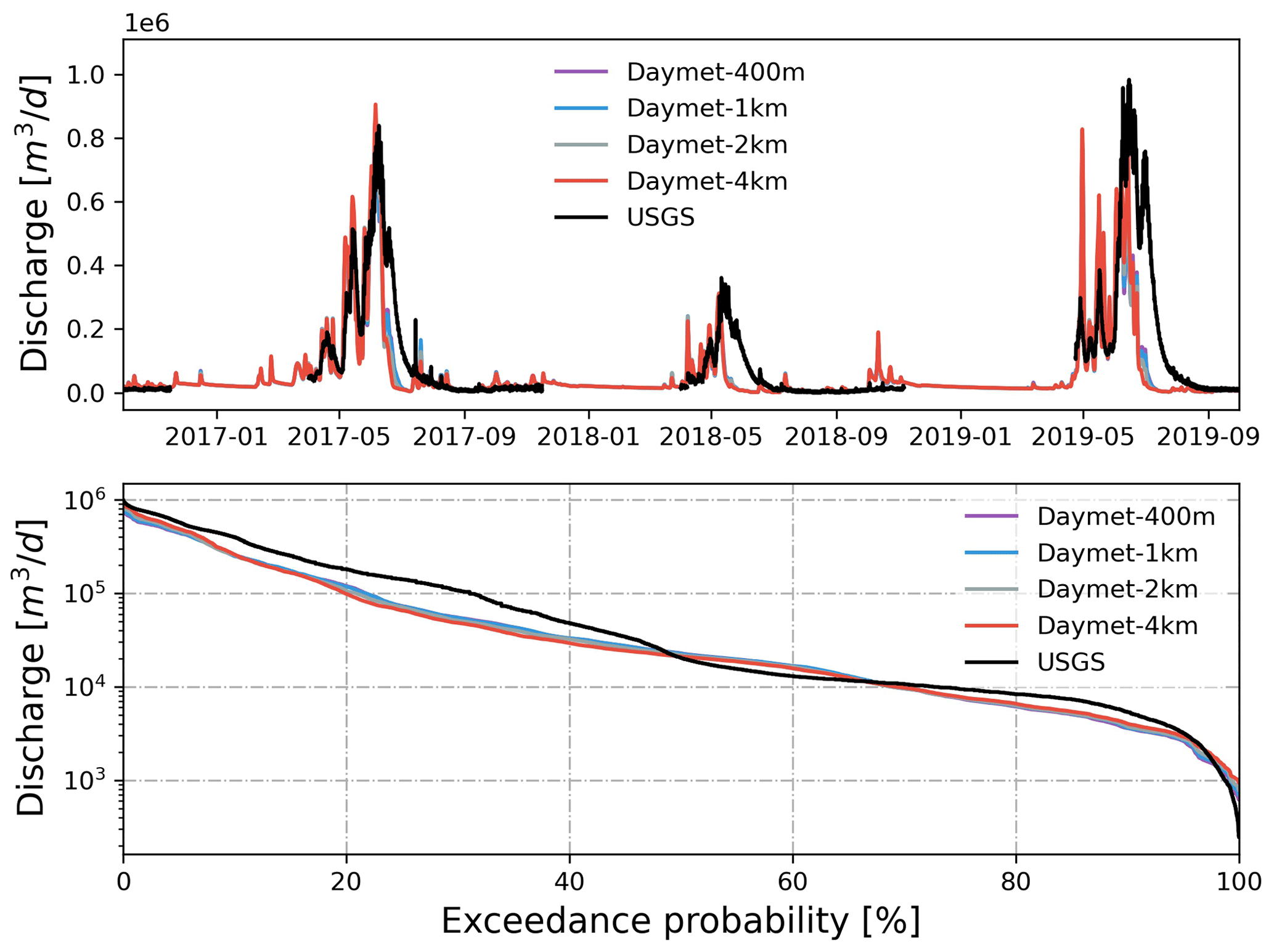
Figure A3 Simulated discharge at the watershed outlet compared to the USGS gage under different spatial resolutions of Daymet. Also shown is the flow duration curve comparison.

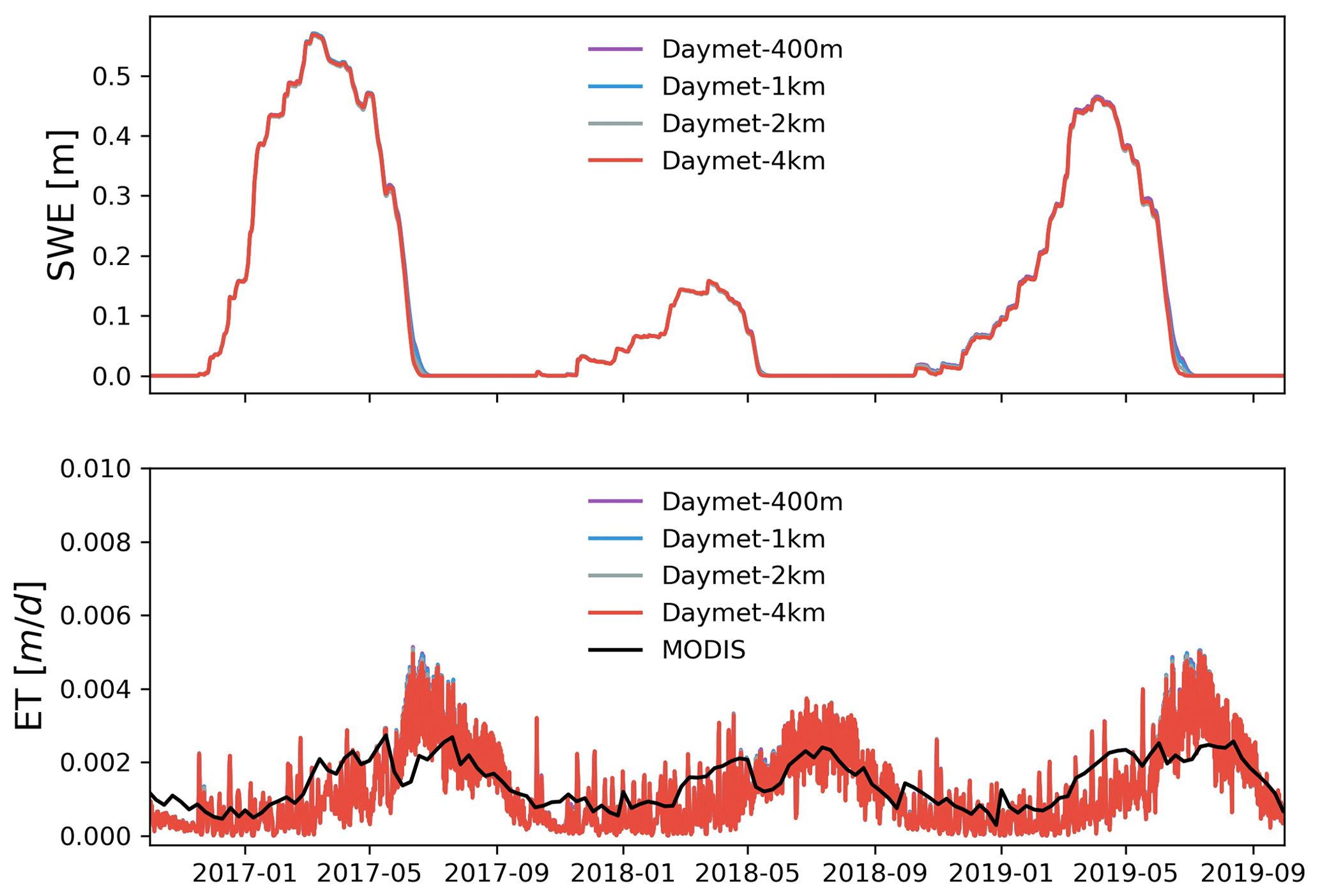
Figure A4 Simulated watershed average SWE and ET under different spatial resolutions of Daymet.

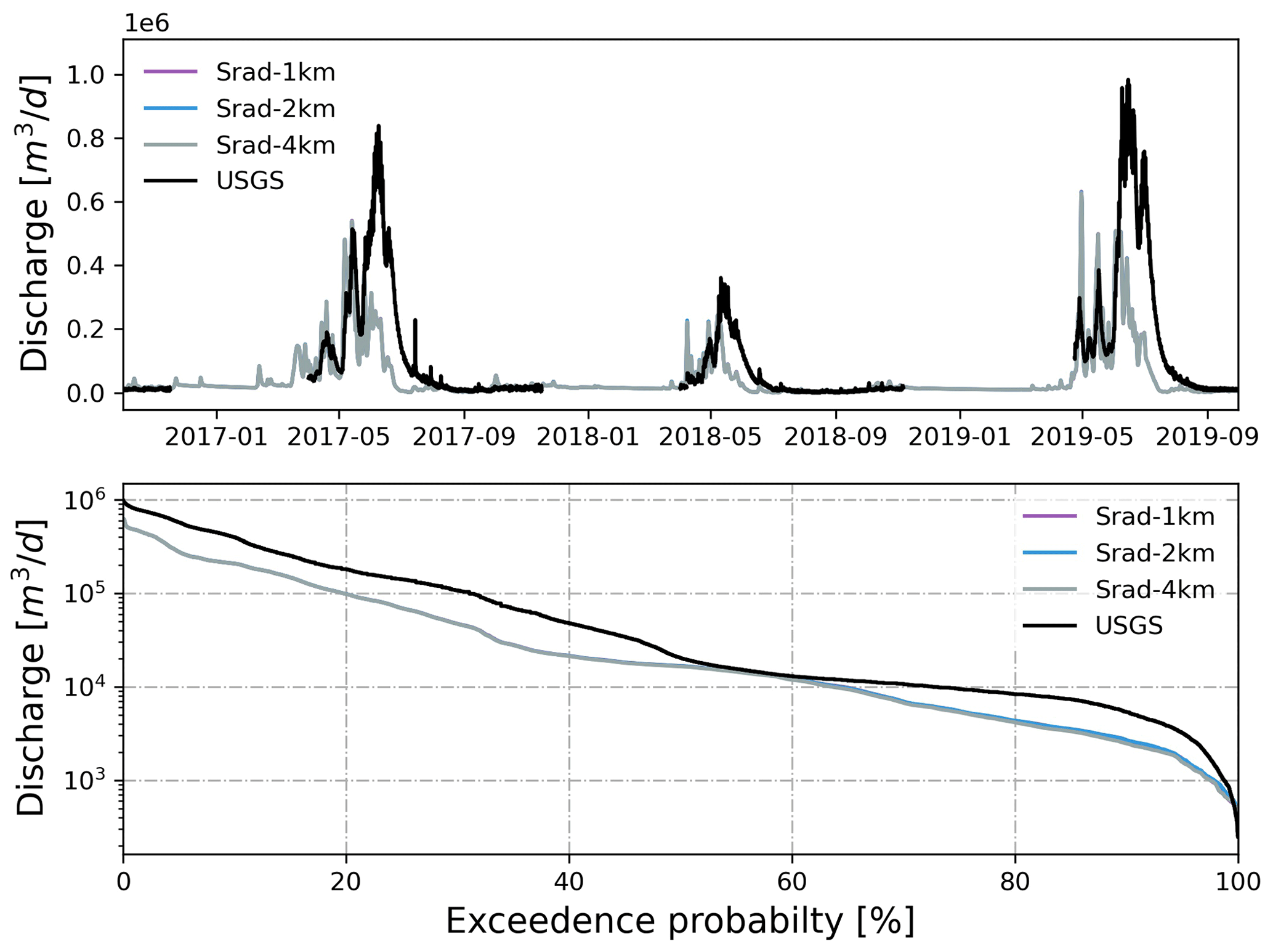
Figure A5 Simulated watershed outlet discharge under different spatial resolutions of S_rad. Also shown is the flow duration curve comparison.

A4 Impact of spatial and temporal resolution of solar radiation

The effect of solar radiation (i.e., S_rad) spatial resolution was tested using Daymet shortwave radiation at 1, 2, and 4 km resolution while keeping the other forcing variables the same. The effect of solar radiation temporal resolution was tested using NLDAS shortwave radiation at hourly, 12-hourly and daily resolution while keeping other forcings the same. By comparing ET and streamflow, the spatial resolution of shortwave radiation has little impact on ET and streamflow, whereas the temporal resolution of shortwave radiation slightly changed the dynamics of ET and streamflow. Overall watershed responses are less sensitive to solar radiation than precipitation and temperature.

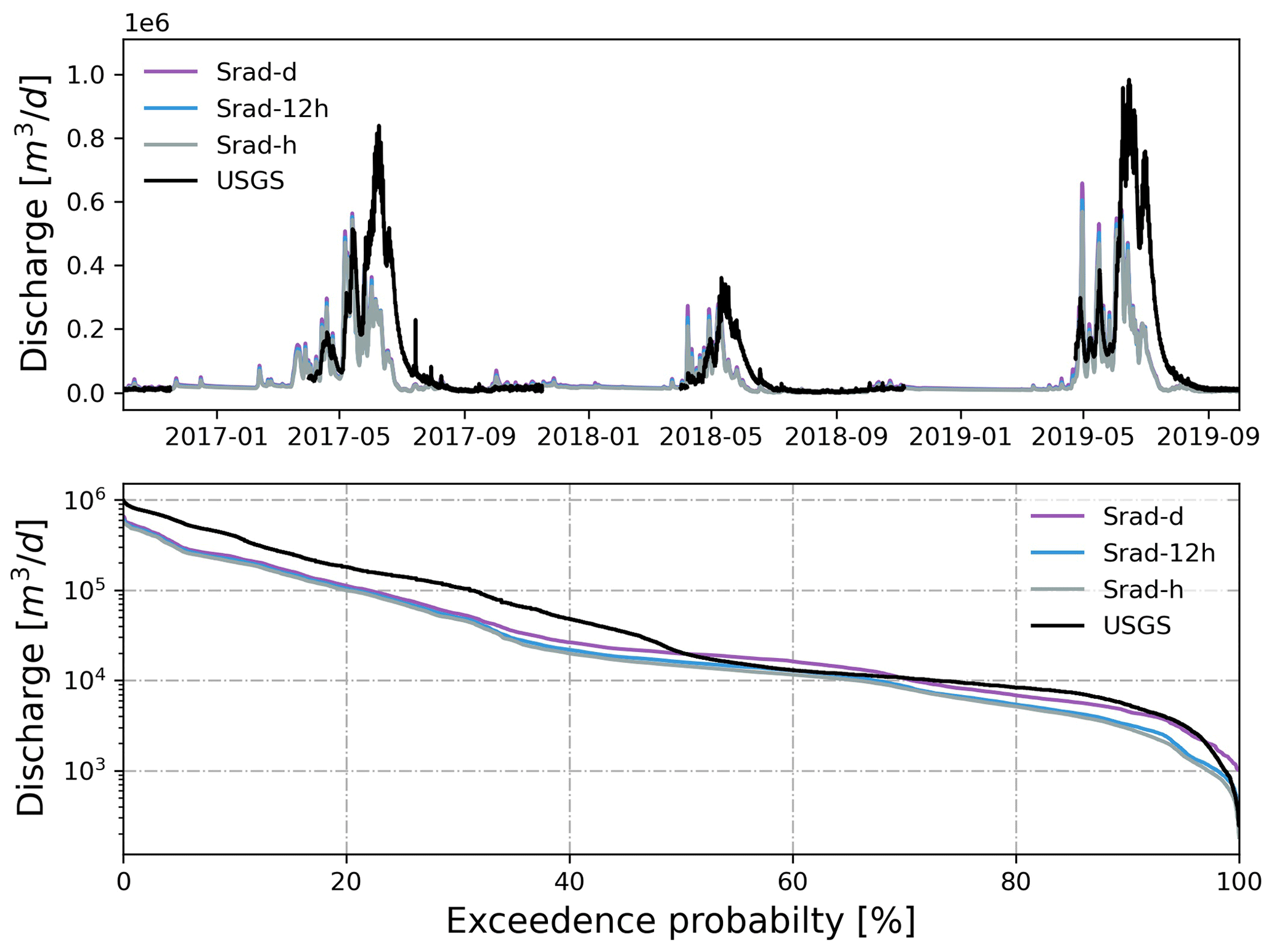
Figure A6 Simulated watershed outlet discharge under different temporal resolutions of S_rad. Also shown is the flow duration curve comparison.

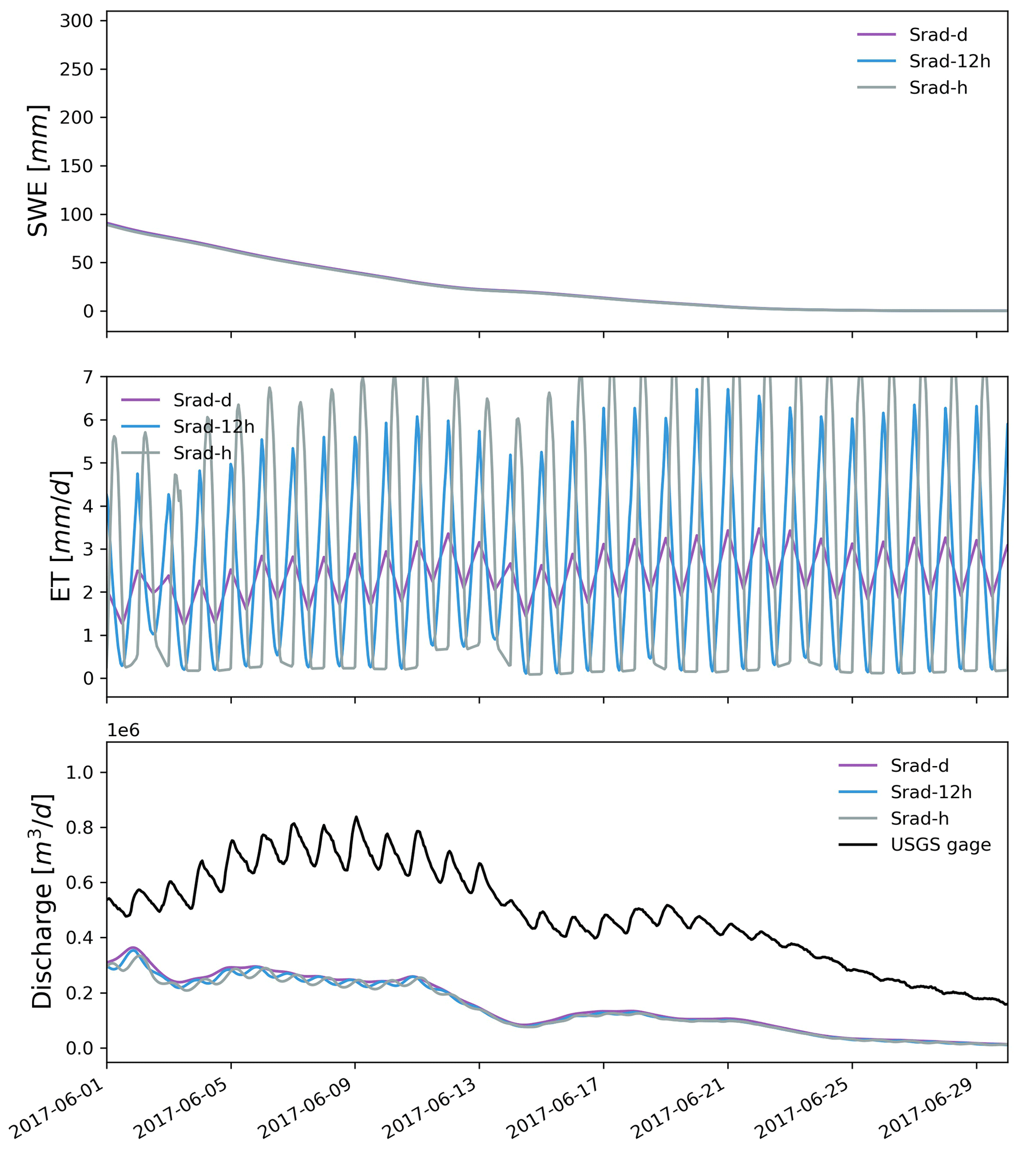
Figure A7 Zoomed-in plots showing simulated SWE, ET, and watershed outlet discharge under different temporal resolutions of S_rad.

A5 Additional results from PRISM comparison under different spatial resolution

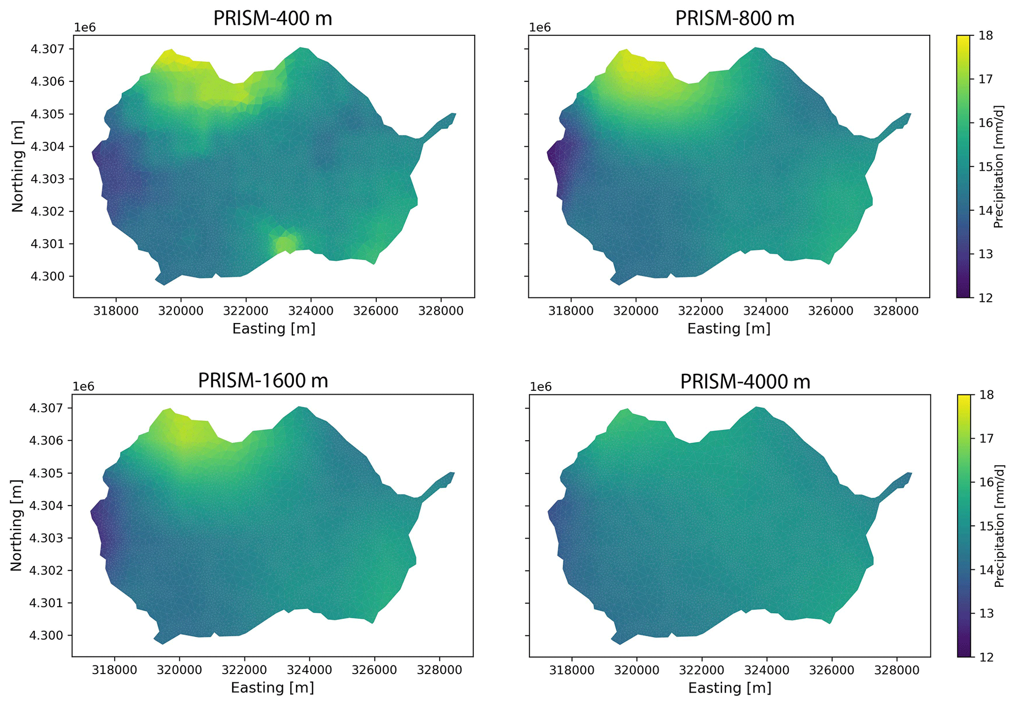
Figure A8 Spatial distribution of precipitation under different spatial resolutions of PRISM on 27 April 2019.

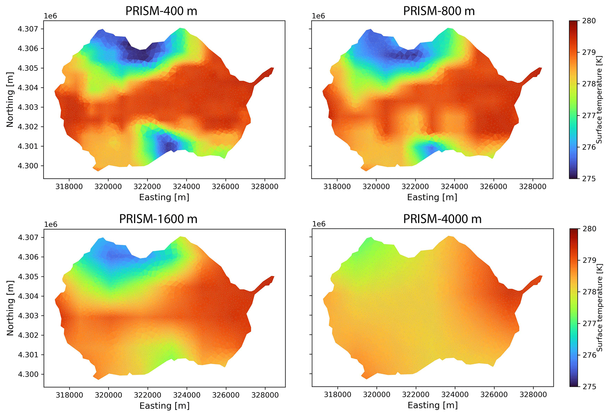
Figure A9 Spatial distribution of air temperature under different spatial resolutions of PRISM on 27 April 2019.

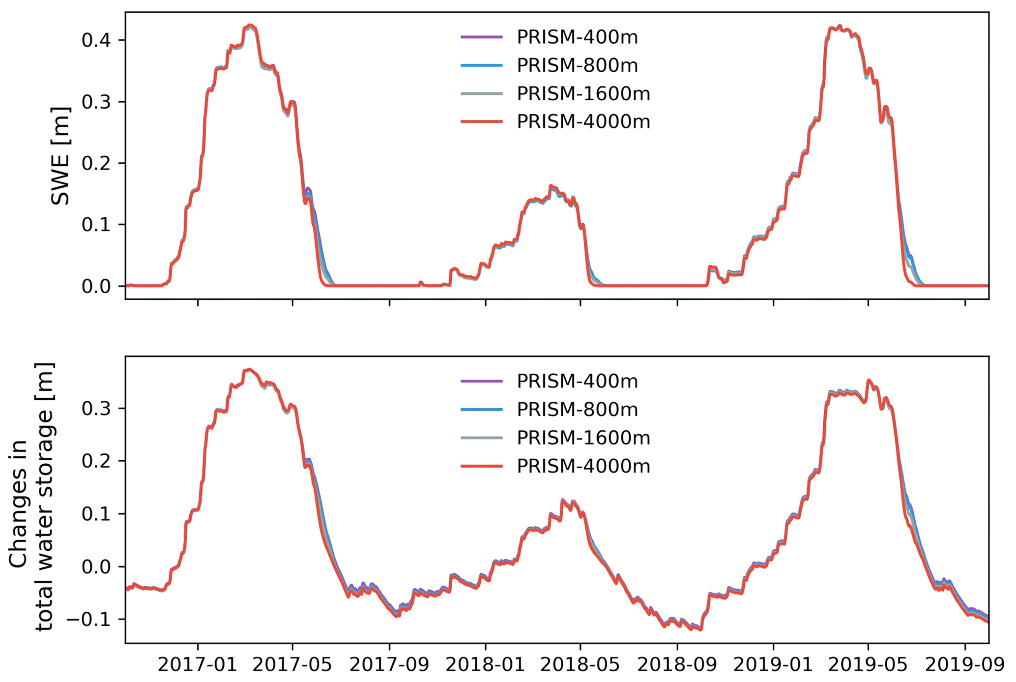
Figure A10 Simulated watershed average SWE and changes in total water storage under different spatial resolutions of PRISM.

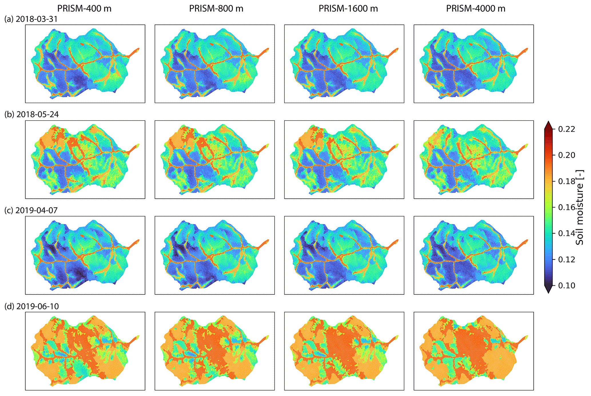
Figure A11 Spatial distribution of soil moisture at land surface under different spatial resolutions of PRISM at four different times.

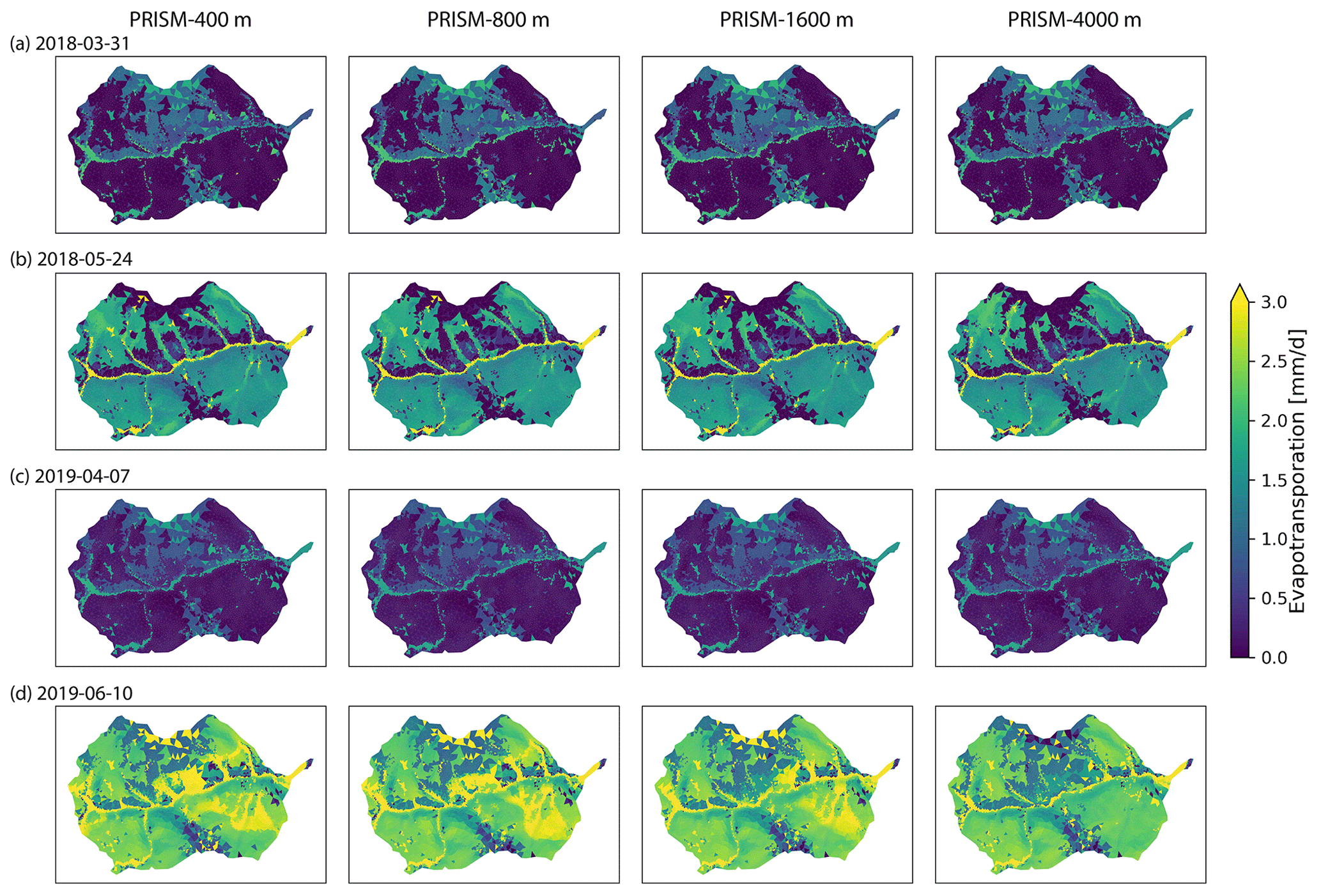
Figure A12 Spatial distribution of ET under different spatial resolutions of PRISM at four different times.