the Creative Commons Attribution 4.0 License.
the Creative Commons Attribution 4.0 License.
 | 31 Mar 2022
Uncertainty estimation with deep learning for rainfall–runoff modeling
Frederik Kratzert
Martin Gauch
Alden Keefe Sampson
Johannes Brandstetter
Günter Klambauer
Sepp Hochreiter
Grey Nearing
Deep learning is becoming an increasingly important way to produce accurate hydrological predictions across a wide range of spatial and temporal scales. Uncertainty estimations are critical for actionable hydrological prediction, and while standardized community benchmarks are becoming an increasingly important part of hydrological model development and research, similar tools for benchmarking uncertainty estimation are lacking. This contribution demonstrates that accurate uncertainty predictions can be obtained with deep learning. We establish an uncertainty estimation benchmarking procedure and present four deep learning baselines. Three baselines are based on mixture density networks, and one is based on Monte Carlo dropout. The results indicate that these approaches constitute strong baselines, especially the former ones. Additionally, we provide a post hoc model analysis to put forward some qualitative understanding of the resulting models. The analysis extends the notion of performance and shows that the model learns nuanced behaviors to account for different situations.
- Article
(2984 KB) - Full-text XML
- BibTeX
- EndNote


A growing body of empirical results shows that data-driven models perform well in a variety of environmental modeling tasks (e.g., Hsu et al., 1995; Govindaraju, 2000; Abramowitz, 2005; Best et al., 2015; Nearing et al., 2016, 2018). Specifically for rainfall–runoff modeling, approaches based on long short-term memory (LSTM; Hochreiter, 1991; Hochreiter and Schmidhuber, 1997; Gers et al., 1999) networks have been especially effective (e.g., Kratzert et al., 2019a, b, 2021).
The majority of machine learning (ML) and deep learning (DL) rainfall–runoff studies do not provide uncertainty estimates (e.g., Hsu et al., 1995; Kratzert et al., 2019b, 2021; Liu et al., 2020; Feng et al., 2020). However, uncertainty is inherent in all aspects of hydrological modeling, and it is generally accepted that our predictions should account for this (Beven, 2016). The hydrological sciences community has put substantial effort into developing methods for providing uncertainty estimations around traditional models, and similar effort is necessary for DL models like LSTMs.
Currently there exists no single, prevailing method for obtaining distributional rainfall–runoff predictions. Many, if not most, methods take a basic approach where a deterministic model is augmented with some uncertainty estimation strategy. This includes, for example, ensemble-based methods, where the idea is to define and sample probability distributions around different model inputs and/or structures (e.g., Li et al., 2017; Demargne et al., 2014; Clark et al., 2016), but it also comprises Bayesian (e.g., Kavetski et al., 2006) or pseudo-Bayesian (e.g., Beven and Binley, 2014) methods and post-processing methods (e.g., Shrestha and Solomatine, 2008; Montanari and Koutsoyiannis, 2012). In other words, most classical rainfall–runoff models do not provide direct estimates of their own predictive uncertainty; instead, such models are used as a part of a larger framework. There are some exceptions to this, for example, methods based on stochastic partial differential equations, which actually use stochastic models but generally require one to assign sampling distributions a priori (e.g., a Wiener process). These are common, for example, in hydrologic data assimilation (e.g., Reichle et al., 2002). The problem with these types of approaches is that any distribution that we could possibly assign is necessarily degenerate, resulting in well-known errors and biases in estimating uncertainty (Beven et al., 2008).
It is possible to fit DL models such that their own representations intrinsically support estimating distributions while accounting for strongly nonlinear interactions between model inputs and outputs. In this case, there is no requirement to fall back on deterministic predictions that would need to be sampled, perturbed, or inverted. Several approaches to uncertainty estimation for DL have been suggested (e.g., Bishop, 1994; Blundell et al., 2015; Gal and Ghahramani, 2016). Some of them have been used in the hydrological context. For example, Zhu et al. (2020) tested two strategies for using an LSTM in combination with Gaussian processes for drought forecasting. In one strategy, the LSTM was used to parameterize a Gaussian process, and in the second strategy, the LSTM was used as a forecast model with a Gaussian process post-processor. Gal and Ghahramani (2016) showed that Monte Carlo dropout (MCD) can be used to intrinsically approximate Gaussian processes with LSTMs, so it is an open question as to whether explicitly representing the Gaussian process is strictly necessary. Althoff et al. (2021) examined the use of MCD for an LSTM-based model of a single river basin and compared its performance with the usage of an ensemble approach. They report that MCD had uncertainty bands that are more reliable and wider than the ensemble counterparts. This finding contradicts the preliminary results of Klotz et al. (2019) and observations from other domains (e.g., Ovadia et al., 2019; Fort et al., 2019). It is therefore not yet clear whether the results of Althoff et al. (2021) are confined to their setup and data. Be that as it may, this still is evidence of the potential capabilities of MCD. A further use case was examined by Fang et al. (2019), who use MCD for soil moisture modeling. They observed a tendency in MCD to underestimate uncertainties. To compensate, they tested an MCD extension, proposed by Kendall and Gal (2017), the core idea of which is to add an estimation for the aleatoric uncertainty by using a Gaussian noise term. They report that this combination was more effective at representing uncertainty.
Our primary goal is to benchmark several methods for uncertainty estimation in rainfall–runoff modeling with DL. We demonstrate that DL models can produce statistically reliable uncertainty estimates using approaches that are straightforward to implement. We adapted the LSTM rainfall–runoff models developed by Kratzert et al. (2019b, 2021) with four different approaches to make distributional predictions. Three of these approaches use neural networks to create and mix probability distributions (Sect. 2.3.1). The fourth is MCD, which is based on direct sampling from the LSTM (Sect. 2.3.2).
Our secondary objective is to help advance the state of community model benchmarking to include uncertainty estimation. We want to do so by outlining a basic skeleton for an uncertainty-centered benchmarking procedure. The reason for this is that it was difficult to find suitable benchmarks for the DL uncertainty estimation approaches we want to explore. Ad hoc benchmarking and model intercomparison studies are common (e.g., Andréassian et al., 2009; Best et al., 2015; Kratzert et al., 2019b; Lane et al., 2019; Berthet et al., 2020; Nearing et al., 2018), and, while the community has large-sample datasets for benchmarking hydrological models (Newman et al., 2017; Kratzert et al., 2019b), we lack standardized, open procedures for conducting comparative uncertainty estimation studies. For example, from the given references only, Berthet et al. (2020) focused on benchmarking uncertainty estimation strategies, and then only for assessing post-processing approaches. Furthermore, it has previously been argued that data-based models provide a meaningful and general benchmark for testing hypotheses and models (Nearing and Gupta, 2015; Nearing et al., 2020b). Thus, here we examine a data-based uncertainty estimation benchmark built on a standard, publicly available, large-sample dataset that could be used as a baseline for future benchmarking studies.
To carve out a skeleton for a benchmarking procedure, we followed the philosophy outlined by Nearing et al. (2018). According to the principles therein, the requirements for a suitable, standardized benchmark are (i) that the benchmark uses a community-standard dataset that is publicly available, (ii) that the model or method is applied in a way that conforms to the standards of practice for that dataset (e.g., standard train/test splits), and (iii) that the results of the standardized benchmark runs are publicly available. To these, we added a fourth point, a post hoc model examination step which aims at exposing the intrinsic properties of the model. Although examination is important – especially for ML approaches and imperfect approximations – we do not view it as a requirement for benchmarking in general.
Nonetheless, we believe that good benchmarking is not something that can be done in a responsible way by a single contribution (unless it is the outcome of a larger effort in itself, e.g., Best et al., 2015; Kratzert et al., 2019b). In general, however, it will require a community-based effort. If no benchmarking effort is established yet, one would ideally start with a set of self-contained baselines and openly share settings, data, models, and metrics. Then, over time, a community can establish itself and improve, replace, or add to them. In the best case, everyone runs the model or approach that they know best, and results are compared at a community level.
The current study can be seen as a starting point for this process: we base the setup for a UE benchmark on a large, publicly curated, open dataset that is already established for other benchmarking efforts – namely the Catchment Attributes and MEteorolgoical Large Sample (CAMELS) dataset. Section 2.1 provides an overview of the CAMELS dataset. The following sections describe the benchmarking setup: Sect. 2.2 discusses a suite of performance metrics that we used to evaluate the uncertainty estimation approaches. Section 2.3 introduces the different uncertainty estimation baselines that we developed. We used exclusively data-driven models because they capture the empirically inferrable relationships between inputs and outputs (and assume minimal a-priori process conceptualization; see, e.g., Nearing et al., 2018, 2020b). The setup, the models, and the metrics should be seen as a minimum viable implementation of a comparative examination of uncertainty predictions, a template that can be expanded and adapted to progress benchmarking in a community-minded way. Lastly, Sect. 2.4 discusses the different experiments of the post hoc model examination. Our goal here is to make the behavior and performance of the (best) model more tangible and compensate for potential blind spots of the metrics.
2.1 Data: the CAMELS dataset
CAMELS (Newman et al., 2015; Addor et al., 2017) is an openly available dataset that contains basin-averaged daily meteorological forcings derived from three different gridded data products for 671 basins across the contiguous United States. The 671 CAMELS basins range in size between 4 and 25 000 km2 and span a range of geological, ecological, and climatic conditions. The original CAMELS dataset includes daily meteorological forcings (precipitation, temperature, short-wave radiation, humidity) from three different data sources (NLDAS, Maurer, DayMet) for the time period 1980 through 2010 as well as daily streamflow discharge data from the US Geological Survey. CAMELS also includes basin-averaged catchment attributes related to soil, geology, vegetation, and climate.
We used the same 531 basins from the CAMELS dataset (Fig. 1) that were originally chosen for model benchmarking by Newman et al. (2017). This means that all basins from the original 671 with areas greater than 2000 km2 or with discrepancies of more than 10 % between different methods for calculating basin area were not considered. Since all of the models that we tested here are DL models, we use the terms training, validation, and testing, which are standard in the machine learning community, instead of the terms calibration and validation, which are more common in the hydrology community (sensu Klemeš, 1986).
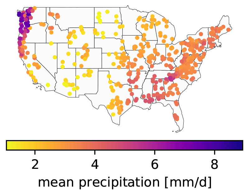
Figure 1Overview map of the CAMELS basins. The plot shows the mean precipitation estimates for the 531 basins originally chosen by Newman et al. (2017) and used in this study.
2.2 Metrics: benchmarking evaluation
Benchmarking requires metrics to evaluate. No global, unique metric exists that is able to fully capture model behavior. As a matter of fact, it is often the case that even multiple metrics will miss important aspects. The choice of metrics will also necessarily depend on the goal of the benchmarking exercise. Post hoc model examination provides a partial remedy to these inefficiencies by making the model behavior more tangible. Still, as of now, no canonical set of metrics exists. The ones we employed should be seen as a bare minimum, a starting point so to speak. The metrics will need to be adapted and refined over time and from application to application.
The minimal metrics for benchmarking uncertainty estimations need to test whether the distributional predictions are “reliable” and have “high resolution” (a terminology we adopted from Renard et al., 2010). Reliability measures how consistent the provided uncertainty estimates are with respect to the available observations, and resolution measures the “sharpness” of distributional predictions (i.e., how thin the body of the distribution is). Generally, models with higher resolution are preferable. However, this preference is conditional on the models being reliable. A model should not be overly precise relative to its accuracy (over-confident) or overly disperse relative to its accuracy (under-confident). Generally speaking, a single metric will not suffice to completely summarize these properties (see, e.g., Thomas and Uminsky, 2020). We note however that the best form metrics for comparing distributional predictions would be to use proper scoring rules, such as likelihoods (see, e.g., Gneiting and Raftery, 2007). Likelihoods however do not exist on an absolute scale (it is generally only possible to compare likelihoods between models), which makes these difficult to interpret (although see Weijs et al., 2010). Additionally, these can be difficult to compute with certain types of uncertainty estimation approaches and so are not completely general for future benchmarking studies. To have a minimal viable set of metrics, we therefore based the assessment of reliability on probability plots and evaluated resolution with a set of summary statistics.
All metrics that we report throughout the paper are evaluated on the test data only. With that we follow the thoughts outlined by Klemeš (1986) and the current established practice in machine learning.
2.2.1 Reliability
Probability plots (Laio and Tamea, 2007) are based on the following observation: if we insert the observations into the estimated cumulative distribution function, a consistent model will provide a uniform distribution on the interval [0, 1]. The probability plot uses this to provide a diagnostic. The theoretical quantiles of this uniform distribution are plotted on the x axis and the fraction of observations that fall below the corresponding predictions on the y axis (Fig. 2). Deficiencies appear as deviations from the 1:1 line: a perfect model should capture 10 % of the observations below a 10 % threshold, 20 % under the 20 % threshold, and so on. If the relative counts of observations, in particular modeled quantiles, are higher than the theoretical quantiles, this means that a model is under-confident. Similarly, if the relative counts of observations, in particular modeled quantiles, are lower than the theoretical quantiles, then the model is over-confident.
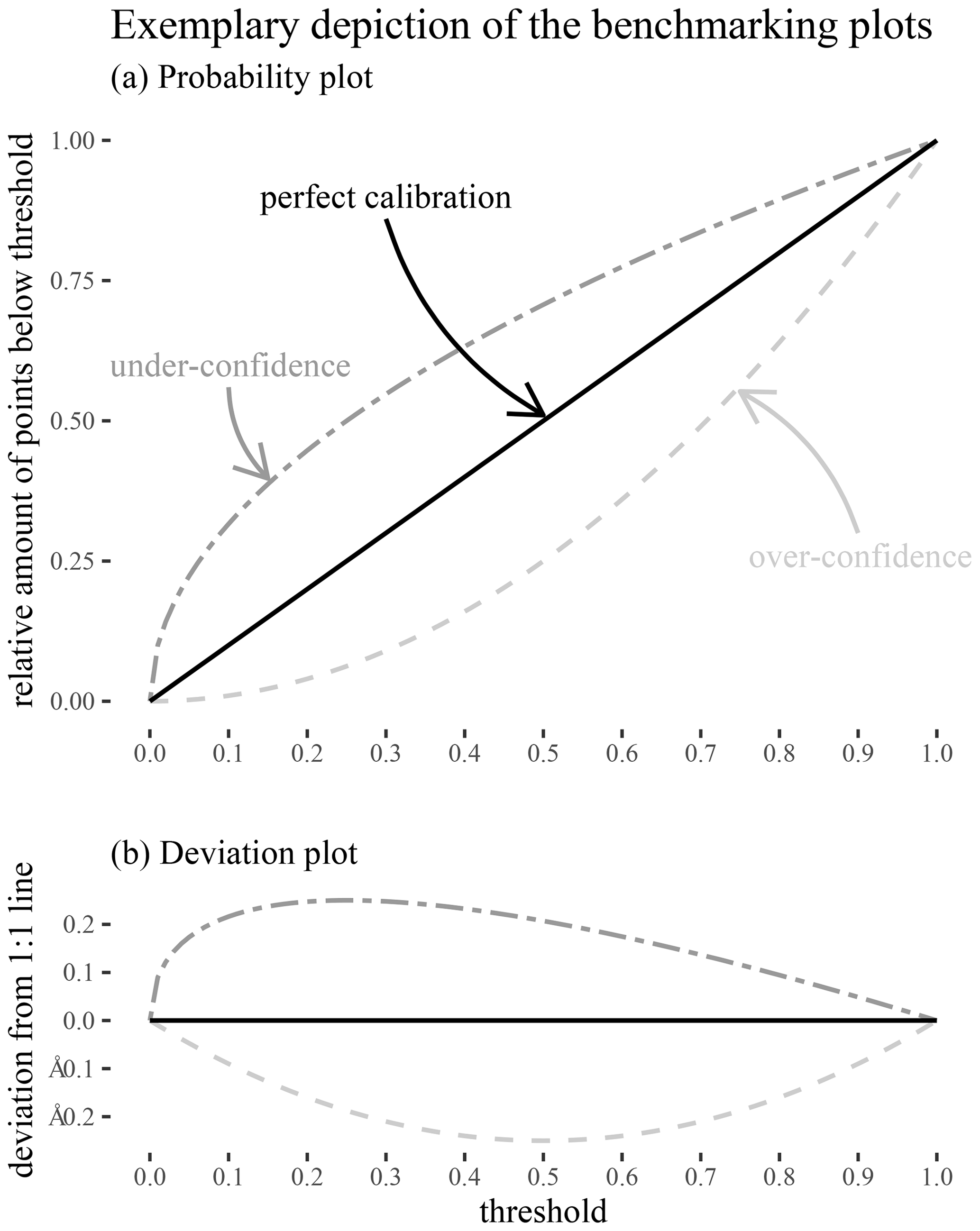
Figure 2(a) Illustration of the probability plot for the evaluation of predictive distributions. The x axis shows the estimated cumulative distribution over all time steps by a given model, and the y axis shows the actual observed cumulative probability distribution. A conditional probability distribution was produced by each model for each time step in each basin. A hypothetically perfect model will have a probability plot that falls on the 1:1 line. We used 10 % binning in our actual experiments. (b) Illustration of the corresponding “error plot”. This plot complements the probability by explicitly depicting the distances of individual models from the 1:1 line.
Laio and Tamea (2007) proposed using the probability plot in a continuous fashion to avoid arbitrary binning. We preferred to use discrete steps in our quantile estimates to avoid falsely reporting overly precise results (e.g., Cole, 2015). As such, we chose a 10 % step size for the binning thresholds in our experiments. We used 10 thresholds in total, one for each of the resulting steps and the additional 1.0 threshold which used the highest sampled value as an upper bound, so that an intuition regarding the upper limit can be obtained. Subtracting the thresholds from the relative count yields a deviation from the 1:1 line (the sum of which is sometimes referred to as the expected calibration error; see, e.g., Naeini et al., 2015). For the evaluation we depicted this counting error alongside the probability plots to provide better readability (see Fig. 2b).
A deficit of the probability plot is its coarseness, since it represents an aggregate over time and basins. As such, it provides a general overview but necessarily neglects many aspects of hydrological importance. Many expansions of the analytical range are possible. One that suggested itself was to examine the deviations from the 1:1 line for different basins. Therefore, we evaluated the probability plot for each basin specifically, computed the deviations from the 1:1 line, and examined their distributions. We did not include the 1.0 threshold for this analysis since it consisted of large spikes only.
2.2.2 Resolution
To motivate why further metrics are required on top of the reliability plot, it is useful to look at the following observation: there are an infinity of models that produce perfect probability plots. One edge-case example is a model that simply ignores the inputs and produces the unconditional empirical data distribution at every time step. Another edge-case example is a hypothetical “perfect” model that produces delta distributions at exactly the observations every time. Both of these models have precision that exactly matches accuracy, and these two models could not be distinguished from each other using a probability plot. Similarly, a model which is consistently under-confident for low flows can compensate for this by being over-confident for higher flows. Thus, to better assess the uncertainty estimations, at least another dimension of the problem has to be checked: the resolution.
Table 1Overview of the benchmarking metrics for assessing model resolution. Each metric is applied to the distributional streamflow predictions at each individual time step and then aggregated over all time steps and basins. All metrics are defined in the interval [0, ∞), and lower values are preferable (but not unconditional on the reliability).
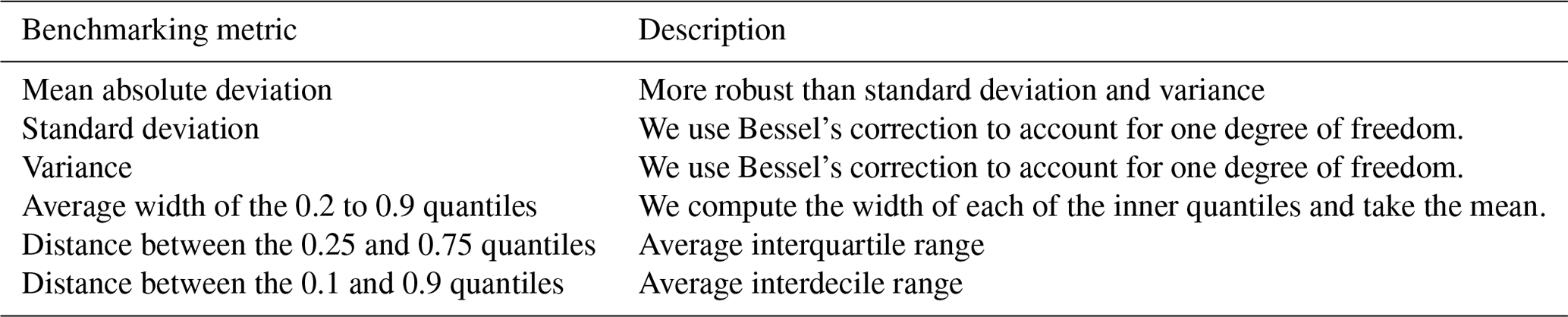
To assess the resolution of the provided uncertainty estimates, we used a group of metrics (Table 1). Each metric was computed for all available data points and averaged over all time steps and basins. The results are statistics that characterize the overall sharpness of the provided uncertainty estimates (roughly speaking, they give us a notion about how thin the body of the distributional predictions is). Further, to provide an anchor for interpreting the magnitudes of the statistics, we also computed them for the observed streamflow values (this yields an unconditional empirical distribution for each basin that can be aggregated). These are not strictly the same, but we argue that they still provide some form of guidance.
2.3 Baselines: uncertainty estimation with deep learning
We tested four strategies for uncertainty estimation with deep learning. These strategies fall into two broad categories: mixture density networks (MDNs) and MCD. We argue that these approaches represent a useful set of baselines for benchmarking.
2.3.1 Mixture density networks
The first class of approaches uses a neural network to mix different probability densities. This class is commonly referred to as MDNs (Bishop, 1994), and we tested three different forms of MDNs. A mixture density is a probability density function created by combining multiple densities, called components. An MDN is defined by the parameters of each component and the mixture weights. The mixture components are usually simple distributions like the Gaussians in Fig. 3. Mixing is done using weighted sums. Mixture weights are larger than zero and collectively sum to one to guarantee that the mixture is also a density function. These weights can therefore be seen as the probability of a particular mixture component. Usually, the number of mixture components is discrete; however, this is not a strict requirement.
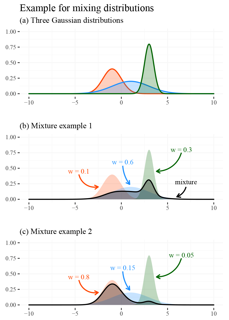
Figure 3Illustration of the concept of a mixture density using Gaussian distributions. Plot (a) shows three Gaussian distributions with different parameters (i.e., different means and standard deviations). Plot (b) shows the same distributions superimposed with the mixture that results from the depicted weighting . Plot (c) shows the same juxtaposition, but the mixture is derived from a different weighting . The plots demonstrate that even in the simple example with fixed parameters the skewness and form of the mixed distribution can vary strongly.
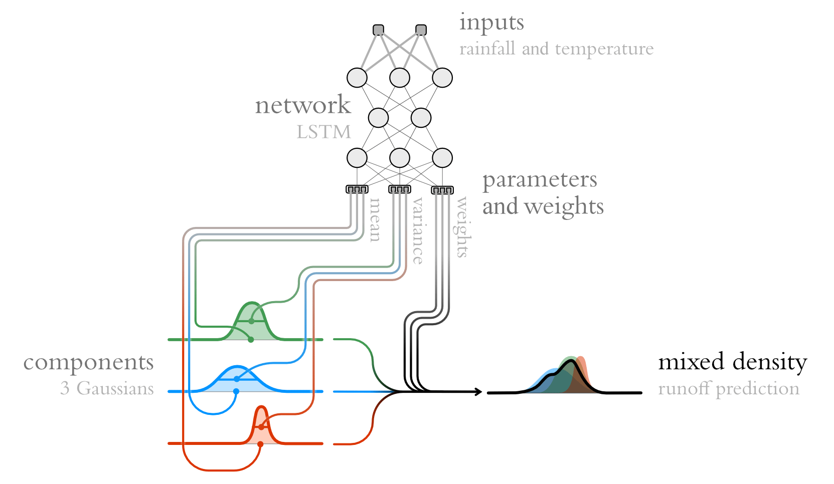
Figure 4Illustration of a mixture density network. The core idea is to use the outputs of a neural network to determine the mixture weights and parameters of a mixture of densities (see Fig. 3). That is, for a given input, the network determines a conditional density function, which it builds by mixing a set of predefined base densities (the so-called components).
The output of an MDN is an estimation of a conditional density, since the mixture directly depends on a given input (Fig. 4). The mixture represents changes every time the network receives new inputs (i.e., in our case for every time step). We thus obtain time-varying predictive distributions that can approximate a large variety of distributions (they can, for example, account for asymmetric and multimodal properties). The resulting model is trained by maximizing the log-likelihood function of the observations according to the predicted mixture distributions. We view MDNs as intrinsically distributional in the sense that they provide probability distributions instead of first making deterministic streamflow estimates and then appending a sampling distribution.
In this study, we tested three different MDN approaches.
-
Gaussian mixture models (GMMs) are MDNs with Gaussian mixture components. Appendix B1 provides a more formal definition as well as details on the loss/objective function.
-
Countable mixtures of asymmetric Laplacians (CMAL) are similar to GMMs, but instead of Gaussians, the mixture components are asymmetric Laplacian distributions (ALDs). This allows for an intrinsic representation of the asymmetric uncertainties that often occur with hydrological variables like streamflow. Appendix B2 provides a more formal description as well as details on the loss/objective function.
-
Uncountable mixtures of asymmetric Laplacians (UMAL) also use asymmetric Laplacians as mixture components, but the mixture is not discretized. Instead, UMAL approximates the conditional density by using Monte Carlo integration over distributions obtained from quantile regression (Brando et al., 2019). Appendix B3 provides a more formal description as well as details on the loss/objective function.
One can read this enumeration as a transition from simple to complex: we start with Gaussian mixture components, then replace them with ALD mixture components, and lastly transition from a fixed number of mixture components to an implicit approximation. There are two reasons why we argue that the more complex MDN methods might be more promising than a simple GMM. First, error distributions in hydrologic simulations often have heavy tails. A Laplacian component lends itself to thicker-tailed uncertainty (Fig. 5). Second, streamflow uncertainty is often asymmetrical, and thus the ALD component could make more sense than a symmetric distribution in this application. For example, even a single ALD component can be used to account for zero flows (compare Fig. 5b). UMAL extends this to avoid having to pre-specify the number of mixture components, which removes one of the more subjective degrees of freedom from the model design.
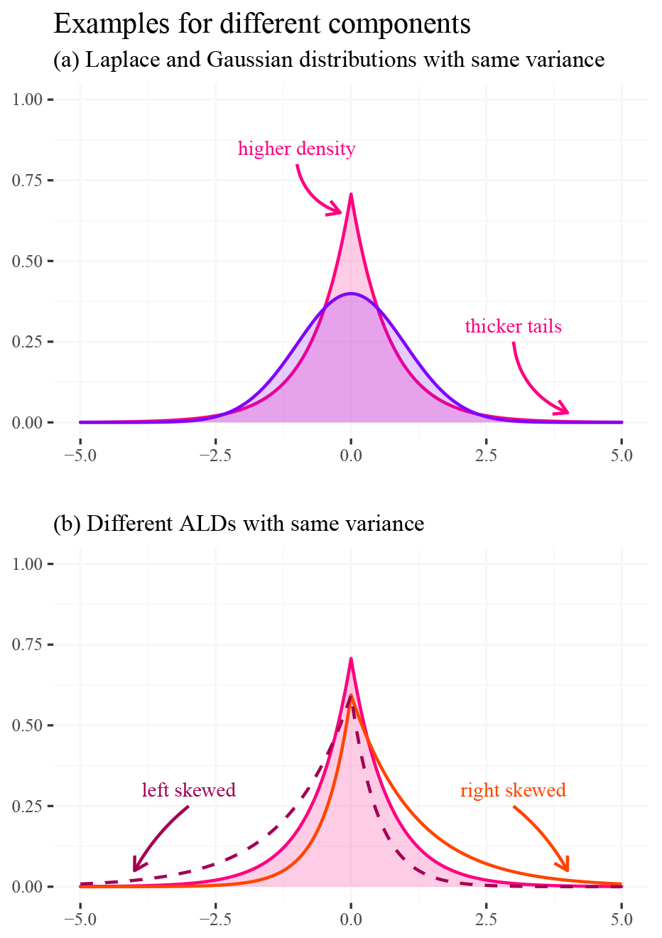
Figure 5Characterization of distributions that are used as mixture components in our networks. Plot (a) superimposes a Gaussian with a Laplacian distribution. The latter is sharper around its center, but this sharpness is traded with thicker tails. We can think about it in the following way: the difference in area is moved to the center and the tails of the distributions. Plot (b) illustrates how the asymmetric Laplacian distribution (ALD) can accommodate for differences in skewness (via an additional parameter).
2.3.2 Monte Carlo dropout
MCD provides an approach to estimate a basic form of epistemic uncertainty. In the following we provide the intuition behind its application.
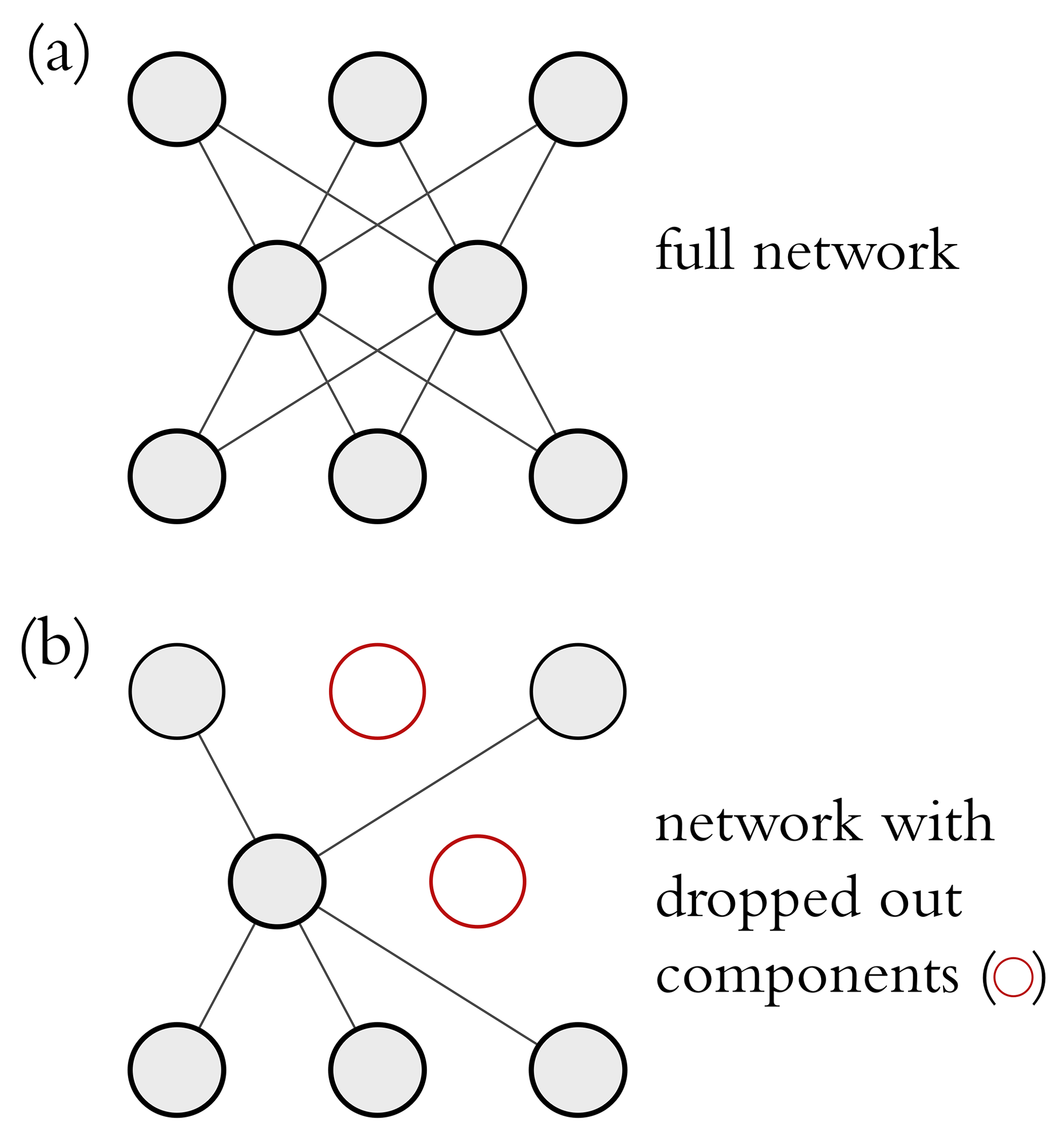
Dropout is a regularization technique for neural networks but can also be used for uncertainty estimation (Gal and Ghahramani, 2016). Dropout randomly ignores specific network units (see Fig. 6). Hence, each time the model is evaluated during training, the network structure is different. Repeating this procedure many times results in an ensemble of many submodels within the network. Dropout regularization is used during training, while during the model evaluation the whole neural network is used. Gal and Ghahramani (2016) showed that dropout can be used as a sampling technique for Bayesian inference – hence the name Monte Carlo dropout.
2.3.3 Model setup
All models are based on the LSTMs from Kratzert et al. (2021). We configured them so that they use meteorological variables as input and predict the corresponding streamflow. This implies that all presented results are from simulation models sensu Beven and Young (2013); i.e., no previous discharge observations were used as inputs. The LSTM in the context of hydrology is inter alia described in Kratzert et al. (2018) and is not repeated here. However, all models can be adapted to a forecasting setting.
In short, our setting was the following. Each model takes a set of meteorological inputs (namely, precipitation, solar radiation, minimum and maximum daily temperature, and vapor pressure) from a set of products (namely, NLDAS, Maurer, and DayMet). As in our previous studies, a set of static attributes is concatenated to the inputs (see Kratzert et al., 2019b). The training period is from 1 October 1980 to 30 September 1990. The validation period is from 1 October 1990 to 30 September 1995. Finally, the test period is from 1 October 1995 to 1 September 2005. This means that we use around training points from 531 catchments (equating to a total of observations for training).
For all MDNs we introduced an additional hidden layer to provide more flexibility and adapted the network as required (see Appendix B). We trained all MDNs with the log-likelihood and the MCD as in Kratzert et al. (2021), except that the loss was the mean squared error (as proposed by Gal and Ghahramani, 2016). All hyperparameters were selected on the basis of the training data, so that they provide the smallest average deviation from the 1:1 line of the probability plot for each model. For GMMs this resulted in 10 components and for CMAL in 3 components (Appendix A).
To make the benchmarking procedure work at the most general level, we employed the setup depicted in Fig. 7. This allows for each approach, with the ability to generate samples, to be plugged into the framework (as evidenced by the inclusion of MCD). For each basin and time step the models either predict the streamflow directly (MCD) or provide a distribution over the streamflow (GMM, CMAL, and UMAL). In the latter case, we then sampled from the distribution to get 7500 sample points for each data point. Since the distributions have infinite support, sampled values below zero cubic meter per day are possible. In this case, we truncated the distribution by setting the sample to 0. All in all, this resulted in simulation points for each model and metric. Exaggerating a little bit, we could say that we actually deal with “multi-point” predictions here.
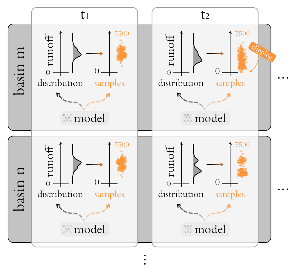
Figure 7Schemata of the general setup. Vertically the procedure is illustrated for two arbitrary basins, m and n, and horizontally the corresponding time steps are depicted. In total we have 531 basins with approximately 3650 data points in time each, and for each time step we compute 7500 samples. In the case of MCD we achieve this by directly sampling from the model. In the case of the MDNs we first estimate a conditional distribution and then sample from it. The “clipping” sign emphasizes our choice to set samples that would be below zero back to the zero-runoff baseline.
2.4 Post hoc model examination: checking model behavior
We performed a post hoc model examination as a complement to the benchmarking to avoid potential blind spots. The analysis has three parts, each one associated with a specific property.
-
Accuracy: how accurate are single-point predictions obtained from the distributional predictions?
-
Internal consistency: how are the mixture components used with regard to flow conditions?
-
Estimation quality: how can we examine the properties of the distributional predictions with regard to second-order uncertainties?
2.4.1 Accuracy: single-point predictions
To address accuracy, we used standard performance metrics applied to single-point predictions (such as the Nash–Sutcliffe efficiency, NSE, and the Kling–Gupta efficiency, KGE; Table 2). The term single-point predictions is used here in the statistical sense of a point estimator to distinguish it from distributional predictions. Single-point predictions were derived as the mean of the distributional predictions at each time step and evaluated for aggregating over the different basins, using the mean and median as aggregation operators (as in Kratzert et al., 2019b). Section 3.2.1 discusses the outcomes of this test as part of the post hoc model examination.
Nash and Sutcliffe (1970)Gupta et al. (2009)Gupta et al. (2009)Gupta et al. (2009)Yilmaz et al. (2008)Yilmaz et al. (2008)Yilmaz et al. (2008)Kratzert et al. (2021)Table 2Overview of the different single-point prediction performance metrics. The table is adapted from Kratzert et al. (2021).

2.4.2 Internal consistency: mixture component behavior
To get an impression of the model consistency, we looked at the behavioral properties of the mixture densities themselves. The goal was to get some qualitative understanding about how the mixture components are used in different situations. As a prototypical example of this kind of examination, we refer to the study of Ellefsen et al. (2019). It examined how LSTMs use the mixture weights to predict the future within a simple game setting. Similarly, Nearing et al. (2020a) reported that a GMM produced probabilities that change in response to different flow regimes. We conducted the same exploratory experiment with the best-performing benchmarked approach.
2.4.3 Estimation quality: second-order uncertainty
MDNs allow a quality check of the given distributional predictions. The basic idea here is that predicted distributions are estimations themselves. MDNs provide an estimation of the aleatoric uncertainty in the data, and the MCD is a basic estimation of the epistemic uncertainty. Thus, the estimations of the uncertainties are not the uncertainties themselves, but – as the name suggests – estimations thereof, and they are thus subject to uncertainties themselves. This does, of course, hold for all forms of uncertainty estimates, not just for MDNs. However, MDNs provide us with single-point predictions of the distribution parameters and mixture weights. We can therefore assess the uncertainty of the estimated mixture components by checking how perturbations (e.g., in the form of input noise) influence the distributional predictions. This can be important in practice. For example, if we mistrust a given input – let us say because the event was rarely observed so far or because we suspect some form of errors – we can use a second-order check to obtain qualitative understanding of the goodness of the estimate.
Concretely, we examined how a second-order effect on the estimated uncertainty can be checked with the MCD approach (which provides estimations for some form of epistemic uncertainties), as it can be layered on top of the MDN approaches (which provide estimations of the aleatoric uncertainties). This means that the Gaussian process interpretation by Gal and Ghahramani (2016) cannot be strictly applied. We can nonetheless use the MCD as a perturbation method, since it still forces the model to learn an internal ensemble.
3.1 Benchmarking results
The probability plots for each model are shown in Fig. 8. The approaches that used mixture densities performed better than MCD, and among all of them, the ones that used asymmetric components (CMAL and UMAL) performed better than GMM. CMAL has the best performance overall. All methods, except UMAL, tend to give estimates above the 1:1 line for thresholds lower than 0.5 (the median). This means that the models were generally under-confident in low-flow situations. GMM was the only approach that showed this type of under-confidence throughout all flow regimes – in other words, GMM was above the 1:1 line everywhere. The largest under-confidence occurred for MCD in the mid-flow range (between the 0.3 and 0.6 quantile thresholds). For higher flow volumes, both UMAL and MCD underestimated the uncertainty. Overall, CMAL was close to the 1:1 line.
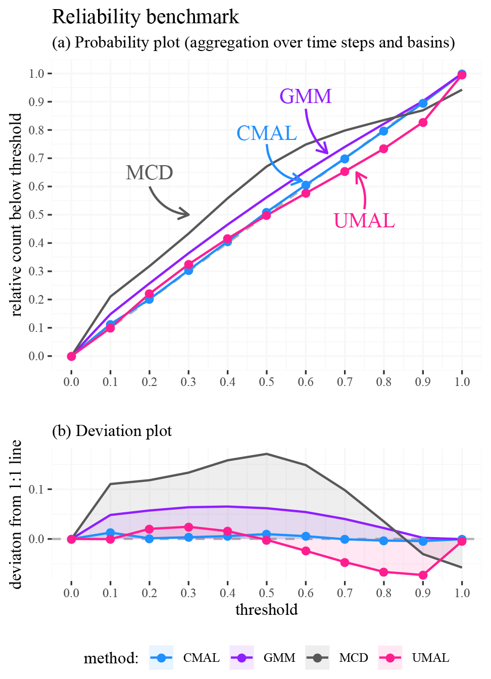
Figure 8Probability plot benchmark results for the 10-year test period over 531 basins in the continental US. Subplot (a) shows the probability plots for the four methods. The 1:1 line is shown in grey and indicates perfect probability estimates. Subplot (b) details deviations from the 1:1 line to allow for easier interpretation.
Figure 9 shows how the deviations from the 1:1 line varied for each basin within each threshold of the probability plot. That is, each subplot shows a specific threshold, and each density resulted from the distributions of deviations from the 1:1 line that the different basins exhibit. The distributions for 0.4 to 0.6 flow quantiles were roughly the same across methods; however, the distributions from CMAL and UMAL were better centered than GMM and MCD. At the outer bounds, a bias was induced due to evaluating in probability space: it is more difficult to be over-confident as the thresholds get lower, and vice versa it is more difficult to be under-confident as the thresholds become higher. At higher thresholds, UMAL had a larger tendency to fall below the center line, which is also visible in the probability plot. Again, this is a consequence of the over-confident predictions from the UMAL approach for larger flow volumes (MCD also exhibited the same pattern of over-confidence for the highest threshold).

Figure 9Kernel densities of the basin-wise deviation from the 1:1 line in the probability plot for the different inner quantiles. These distributions result from evaluating the performance at each basin individually (rather than aggregating over basins). Note how the bounded domain of the probability plot induces a bias for the outer thresholds as the deviations cannot expand beyond the [0, 1] interval.
Table 3Benchmark statistics for model precision. These metrics were applied to the distributional predictions at individual time steps. The lowest metric per row is marked in bold. Lower values are better for all statistics (conditional on the model having high reliability). This table also provides statistics of the empirical distribution from the observations (“Obs”) aggregated over the basins as a reference, which are not directly comparable with the model statistics since “Obs” represents an unconditional density, while the models provide a conditional one. The “Obs” statistics should be used as a reference to contextualize the statistics from the modeled distributions.

* The displayed 0 is a rounding artifact. The actual variance here is higher than 0. The “collapse” is, by and large, a result of a very narrow distribution combined with a heavy truncation for values below 0.
Lastly, Table 3 shows the results of the resolution benchmark. In general, UMAL and MCD provide the sharpest distributions. This goes along with over-confident narrow distributions that both approaches exhibit for high flow volumes. These, having the largest uncertainties, also influence the average resolution the most. The other two approaches, GMM and CMAL, provide lower resolution (less sharp distributions). In the case of GMMs, the low resolution is reflected in under-confidently wide distributions in the probability plot. Notably, the predictions of CMAL are in between those of the over-confident UMAL and the under-confident GMM. This makes sense from a methodological viewpoint since we designed CMAL as an “intermediate step” between the two approaches. Moreover, these results reflect a trade-off in the log-likelihood (which the models are trained for), where a balance between reliability and resolution has to be obtained in order to minimize the loss.
3.2 Post hoc model examination
3.2.1 Accuracy
Table 4 shows accuracy metrics of single-point predictions, i.e., the means of the distributional predictions aggregated over time steps and basins. It depicts the means and medians of each metric across all 531 basins. The approach labeled MCDp reports the statistics from the MCD model but without sampling (i.e., from the full model). The model performances are not entirely comparable with each other, since the architecture and hyperparameters of the MCD model were chosen with regard to the probability plot. We therefore also compare against a model with the same hyper-parameters as Kratzert et al. (2019b) – the latter model is labeled LSTMp in Table 4.
Table 4Evaluation of different single-point prediction metrics. Best performance is marked in bold. Information about the inter-basin variability (dispersion) is provided in the form of the standard deviation whenever the mean is used for aggregation and in the form of the distance to the 25 % and 75 % quantiles when the median is used for aggregation.
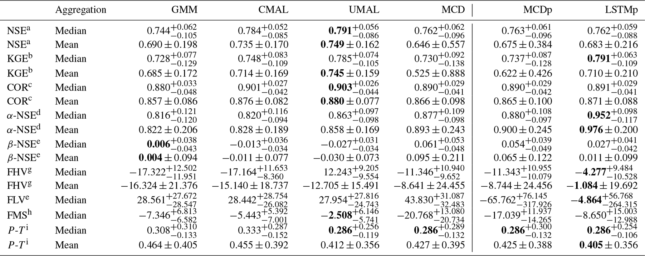
a Nash–Sutcliffe efficiency (−∞, 1]; values closer to 1 are desirable. b Kling–Gupta efficiency (−∞, 1]; values closer to 1 are desirable. c Pearson correlation [−1, 1]; values closer to 1 are desirable. d α-NSE decomposition (0, ∞); values close to 1 are desirable. e β-NSE decomposition (−∞, ∞); values close to 0 are desirable. f Top 2 % peak flow bias (−∞, ∞); values close to 0 are desirable. g 30 % low flow bias (−∞, ∞); values close to 0 are desirable. Since a strong bias is induced by a small subset of basins, we provide the median aggregation. h Bias of the FDC mid-segment slope: (−∞, ∞); values close to 0 are desirable. Since a strong bias is induced by a small subset of basins, we provide the median aggregation. i Peak timing, i.e., lag of peak timing (−∞, ∞); values close to 0 are desirable.
Among the uncertainty estimation approaches, the models with asymmetric mixture components (CMAL and UMAL) perform best. UMAL provided the best point estimates. This is in line with the high resolutions of the uncertainty estimation benchmark: the sharpness makes the mean a better predictor of the likelihood's maximum and indicates again that the approach trades reliability for accuracy. That said, even with our naive approach for obtaining single-point estimations (i.e., simply taking the mean), both CMAL and UMAL manage to outperform the model that is optimized for single-point predictions with regard to some metrics. This suggests that it could make sense to train a model to estimate distributions and then recover the best estimates. One possible reason why this might be the case is that single-point loss functions (e.g., MSE) define an implicit probability distribution (e.g., minimizing an MSE loss is equivalent to maximizing a Gaussian likelihood with fixed variance). Hence, using a more nuanced loss function (i.e., one that is the likelihood of a multimodal, asymmetrical, heterogeneous distribution) can improve performance even for the purpose of making non-distributional estimates. In fact, it is reasonable to expect that the results of the MDN approaches can be improved even further by using a more sophisticated strategy for obtaining single-point predictions (e.g., searching for the maximum of the likelihood). The single-point prediction LSTM (LSTMp) outperforms the ALD-based MDNs for tail metrics of the streamflow – that is, for the low (FLV) and high bias (FHV). These are regimes where we would expect the most asymmetric distributions for hydrological reasons, and hence the means of the asymmetric distributions might be a sub-optimal choice.
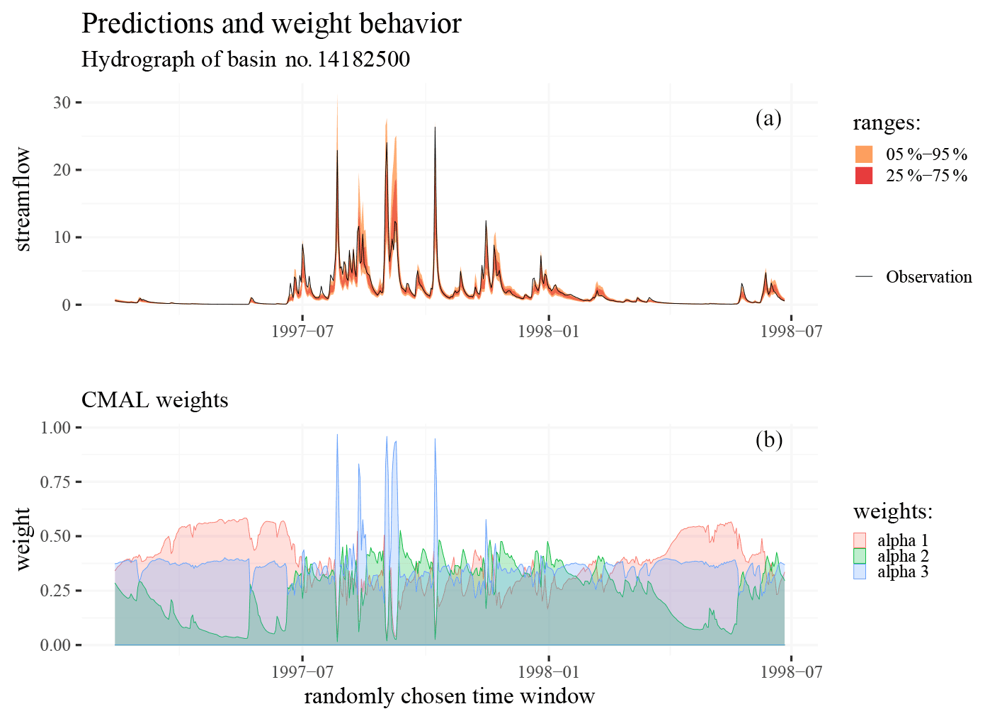
Figure 10(a) Hydrograph of an exemplary event in the test period with both the 5 % to 95 % and 25 % to 75 % quantile ranges. (b) The weights (αi) of the CMAL mixture components for these predictions.
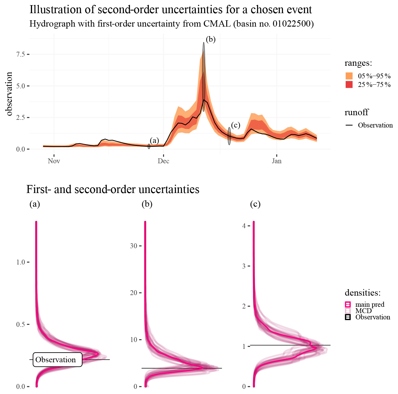
Figure 11Illustration of second-order uncertainties estimated by using MCD to sample the parameters of the CMAL approach. The upper subplot shows an observed hydrograph and predictive distributions as estimated by CMAL. The lower subplots show the CMAL distributions and distributions from 25 MCD samples of the CMAL model at three selected time steps (indicated by black ovals shown on the hydrograph). The abbreviation “main pred” marks the unperturbed distributional predictions from the CMAL model.
3.2.2 Internal consistency
Figure 10 summarizes the behavioral patterns of the CMAL mixture components. It depicts an exemplary hydrograph superimposed on the CMAL uncertainty prediction together with the corresponding mixture component weights. The mixture weights always sum to 1. This figure shows that the model seemingly learns to use different mixture components for different parts of the hydrograph. In particular, distributional predictions in low-flow periods (perhaps dominated by base flow) are largely controlled by the first mixture component (as can be seen by the behavior of mixture α1 in Fig. 10). Falling limbs of the hydrograph (corresponding roughly to throughflow) are associated with the second mixture component (α2), which is low for both rising limbs and low-flow periods. The third component (α3) mainly controls the rising limbs and the peak runoff but also has some influence throughout the rest of the hydrograph. In effect, CMAL learns to separate the hydrograph into three parts – rising limb, falling limb, and low flows – which correspond to the standard hydrological conceptualization. No explicit knowledge of this particular hydrological conceptualization is provided to the model – it is solely trained to maximize overall likelihood.
3.2.3 Estimation quality
In this experiment we want to demonstrate an avenue for studying higher-order uncertainties with CMAL. Intuitively, the distributional predictions are estimations themselves and are thus subject to uncertainty, and, since the distributional predictions do already provide estimates for the prediction uncertainty, we can think about the uncertainty regarding parameters and weights of the components as a second-order uncertainty. In theory even higher-order uncertainties can be thought of. Here, as already described in the Methods section, we use MCD on top of the CMAL approach to “stochasticize” the weights and parameters and expose the uncertainty of the estimations. Figure 11 illustrates the procedure: the upper part shows a hydrograph with the 25 %–75 % quantiles and 5 %–95 % quantiles from CMAL. This is the main prediction. The lower plots show kernel density estimates for particular points of the hydrograph (marked in the upper part with black ovals labeled “a”, “b”, and “c” and shown in red in the lower subplots). These three specific points represent different portions of the hydrograph with different predicted distributional shapes and are thus well suited to showcasing the technique. These kernel densities (in red) are superimposed with 25 sampled estimations derived after applying MCD on top of the CMAL model (shown in lighter tones behind the first-order estimate). These densities are the MCD-perturbed estimations and thus a gauge for how second-order uncertainties influence the distributional predictions.
3.3 Computational demand
This section gives an overview of the computational demand required to compute the different uncertainty estimations. All of the reported execution times were obtained by using NVIDIA P100 (16 GB RAM), using the Pytorch library (Paszke et al., 2019). A single execution of the CMAL model with a batch size of 256 takes s (here, and in the following, the basis gives the median over 100 model runs; the index and the exponent show the deviations of the 10 % quantile and the 90 % quantile, respectively). An execution of the MCD model takes s. The slower execution time of the MCD approach here is explained by its larger hidden size. It used 500 hidden cells, in comparison with the 250 hidden cells of CMAL (see Appendix A).
Generating all the needed samples for the evaluation with MCD and a batch size of 256 would take approximately 36.1 d (since 7500 samples have to be generated for 531 basins and 10 years at a daily resolution). In practice, we could shorten this time to under a week by using considerably larger batch sizes and distributing the computations for different basins over multiple GPUs. In comparison, computing the same number of samples by re-executing the CMAL model would take around 17.4 d. In practice, however, only a single run of the CMAL model is needed, since MDNs provide us with a density estimate from which we can directly sample in a parallel fashion (and without needing to re-execute the model run). Thus, the CMAL model, with a batch size of 256, takes only ∼14 h to generate all needed samples.
Our basic benchmarking scheme allowed us to systematically pursue our primary objective – to examine deep learning baselines for uncertainty predictions. In this regard, we gathered further evidence that deep-learning-based uncertainty estimation for rainfall–runoff modeling is a promising research avenue. The explored approaches are able to provide fully distributional predictions for each basin and time step. All predictions are dynamic: the model adapts them according to the properties of each basin and the current dynamic inputs, e.g., temperature or rainfall. Since the predictions are inherently distributional, the predictions can be further examined and/or reduced to a more basic form, e.g., sample, interval, or point predictions.
The comparative assessment indicated that the MCD approach provided the worst uncertainty estimates. One reason for this is likely the Gaussian assumption of the uncertainty estimates, which seems inadequate for many low- and high-flow situations. There is, however, also a more nuanced aspect to consider: the MDN approaches estimate the aleatoric uncertainty. MCD, on the other hand, estimates epistemic uncertainty, or rather a particular form thereof. The methodological comparison is therefore only partially fair. In general, these two uncertainty types can be seen as perpendicular to each other. They do partially co-appear in our setup, since both the epistemic and aleatoric uncertainties are largest for high flow volumes.
Yet within the chosen setup it was observable that the methods that use inherently asymmetric distributions as components outperformed the other ones. That is, CMAL and UMAL performed better than MCD and GMM in terms of reliability, resolution, and the accuracy of the derived single-point predictions. The CMAL approach in particular gave distributional predictions that were very good in terms of reliability and sharpness (and single-point estimates). There was a direct link between the predicted probabilities and hydrologic behavior in that different distributions were activated (i.e., got larger mixture weights) for rising vs. falling limbs. Nevertheless, likelihood-based approaches (for estimating the aleatoric uncertainty) are prone to giving over-confident predictions. We were not able to diagnose this empirically. This might rather be a result of the limits of the inquiry than the non-existence of the phenomenon.
These limits illustrate how challenging benchmarking is. Rainfall–runoff modeling is a complex endeavor. Unifying the diverse approaches into a streamlined framework is difficult. Realistically, a single research group cannot be able to compare the best possible implementations of the many existing uncertainty estimation schemes – which include approaches such as sampling distributions, ensembles, post-processors, and so forth. We did therefore not only want to examine some baseline models, but also to provide the skeleton for a community-minded benchmarking scheme (see Nearing et al., 2018). We hope this will encourage good practice and provide a foundation for others to build on. As detailed in the Methods section, the scheme consists of four parts. Three of them are core benchmarking components and one is an added model checking step. In the following we provide our main observations regarding each point.
- i.
Data: we used the CAMELS dataset curated by the US National Center for Atmospheric Research and split the data into three consecutive periods (training, validation, and test). All reported metrics are for the test split, which has only been used for the final model evaluation. The dataset has already seen use for other comparative studies and purposes (e.g., Kratzert et al., 2019b, b; Newman et al., 2017). It is also part of a recent generation of open datasets, which we believe are the result of a growing enthusiasm for community efforts. As such, we predict that new benchmarking possibilities will become available in the near future. A downside with using existing open datasets is that the test data are accessible to modelers. This means that a potential defense mechanism against over-fitting on the test data is missing (since the test data might be used during the model selection/fitting process; for broader discussions we refer to Donoho, 2017; Makridakis et al., 2020; Dehghani et al., 2021). To enable rigorous benchmarking, it might thus become relevant to withhold parts of the data and only make them publicly available after some given time (as for example done in Makridakis et al., 2020).
- ii.
Metrics: we put forward a minimal set of diagnostic criteria, that is, a discrete probability plot, obtained from a probability integral transform, for checking prediction reliability, and a set of dispersion metrics to check the prediction resolution (see Renard et al., 2010). Using these, we could see the proposed baselines exhaust the evaluation capacity of these diagnostic tools. On the one hand, this is an encouraging sign for our ability to make reliable hydrologic predictions (the downside being that it might be hard for models to improve on this metric going forward). On the other hand, it is important to be aware that the probability plot and the dispersion statistic miss several important aspects of probabilistic prediction (for example, precision, consistency, or event-specific properties). All reported metrics are highly aggregated summaries (over multiple basins and time steps) of highly nonlinear relationships (see also Muller, 2018; Thomas and Uminsky, 2020). This is compounded by the inherent noise of the data. We therefore expect that many nuanced aspects are missed by the comparative assessment. In consequence, we hope that future efforts will derive more powerful metrics, tests, and probing procedures – akin to the continuous development of diagnostics for single-point predictions (see Nearing et al., 2018).
- iii.
Baselines: we examined four deep-learning-based approaches. One is based on Monte Carlo dropout and three on mixture density networks. We used them to demonstrate the benchmarking scheme and showed its comparative power. This should however only be seen as a starting point. We predict that stronger baselines will emerge in tandem with stronger metrics. From our perspective, there is plenty of room to build better ones. A perhaps self-evident example of the potential of improvements is ensembles: Kratzert et al. (2019b) showed the benefit of LSTM ensembles for single-point predictions, and we assume that similar approaches could be developed for uncertainty estimation. We are therefore sure that future research will yield improved approaches and move us closer to achieving holistic diagnostic tools for the evaluation of uncertainty estimations (sensu Nearing and Gupta, 2015).
- iv.
Model checking: in the post hoc examination step we tested the model performance with regard to point predictions. Remarkably, the results indicate that the distributional predictions are not only reliable and precise, but also yield strong single-point estimates. Additionally, we checked for internal organization principles of the CMAL model. In doing so we showed (a) how the component weighting of a given basin changes in dependence on the flow regime and (b) how higher-order uncertainties in the form of perturbations of the component weights and parameters change the distributional prediction. The showcased behavior is in accordance with basic hydrological intuition. Specific components are used for low and high streamflow. The uncertainty is lowest near 0 and increases with a rise in streamflow. This relationship is nonlinear and not a simple 1:1 depiction. Similarly, additional uncertainties are expected to change the characteristics of the distributional prediction more for high flows than for low flows. By and large, however, this just a start. We argue that post hoc examination will play a central role in future benchmarking efforts.
To summarize, the presented results are promising. Viewed through the lens of community-based benchmarking, we expect progress on multiple fronts: better data, better models, better baselines, better metrics, and better analyses. To road to get there still has many challenges awaiting. Let us overcome them together.
A1 General setup
Table A provides the general setup for the hyperparameter search and model training.
Table A1Overview of the general benchmarking setup.
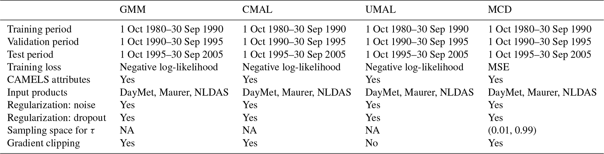
NA stands for not available.
A2 Noise regularization
Adding noise to the data during training can be viewed as a form of data augmentation and regularization that biases towards smooth functions. These are large topics in themselves, and at this stage we refer to Rothfuss et al. (2019) for an investigation on the theoretical properties of noise regularization and some empirical demonstrations. In short, plain maximum likelihood estimation can lead to strong over-fitting (resulting in a spiky distribution that generalizes poorly beyond the training data). Training with noise regularization results in smoother density estimates that are closer to the true conditional density.
Following these findings, we also add noise as a smoothness regularization for our experiments. Concretely, we decided to use a relative additive noise as a first-order approximation to the sort of noise contamination we expect in hydrological time series. The operation for regularization is
where z is a placeholder variable for either the dynamic or static input variables or the observed runoff (and, as before, the time index is omitted for the sake of simplicity), 𝒩(0,σ) denotes a Gaussian noise term with mean zero and a standard deviation σ, and z* is the obtained noise-contaminated variable.
A3 Search
To provide a meaningful comparison, we conducted a hyperparameter search for each of the four conditional density estimators. A hyperparameter search is an extended search (usually computationally intensive) for the best pre-configuration of a machine learning model.
Table A2Search space of the hyperparameter search. The search is conducted in two steps: the variables used in the first step are shown in the top part of the table, and the variables used in the second step are shown in the bottom part and are written in bold.
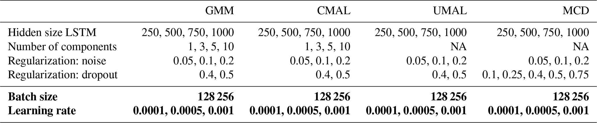
NA stands for not available.
In our case we searched over the combination of six different hyperparameters (see Table A2). To balance between computational resources and search depth, we took the following course of action:
-
First, we informally searched for sensible general presets.
-
Second, we trained the models for each combination of the four hyperparameters “hidden size” (the number of cells in the LSTM; see Kratzert et al., 2019b), “noise” (added relative noise of the output; see Appendix A2), “number of densities” (the number of density heads in the mixture (only needed of MDN and CMAL), and “dropout rate” (the rate of dropout employed during training – and inference in the case of MCD). We marked these in Table A2 with a white background.
-
Third, we choose the best resulting model and refine the found models by searching for the best settings for the hyperparameters “batch size” (the number of samples shown per back-propagation step) and “learning rate” (the parameter for the update per batch).
Table A3Resulting parameterization from the hyperparameter search.

NA stands for not available.
A4 Results
The results of the hyperparameter search are summarized in Table A3.
B1 Gaussian mixture model
Gaussian mixture models (GMMs; Bishop, 1994) are well established for producing distributional predictions from a single input. The principle of GMMs is to have a neural network that predicts the parameters of a mixture of Gaussians (i.e., the means, standard deviations, and weights) and to use these mixtures as distributional output. GMMs are a powerful concept. They have seen usage for diverse applications such as acoustics (Richmond et al., 2003), handwriting generation (Graves, 2013), sketch generation (Ha and Eck, 2017), and predictive control (Ha and Schmidhuber, 2018).
Given the rainfall–runoff modeling context, a GMM models the runoff q∈ℝ at a given time step (subscript omitted for the sake of simplicity) as a probability distribution p(⋅) of the input (where M indicates the number of defined inputs, such as precipitation and temperature and T the number of used time steps which are provided to the neural network) as a mixture of K Gaussians:
where αk are mixture weights with the property αk(x)≥0 and (convex sum), and 𝒩(μk(x),σk(x)) denotes a Gaussian with mean μk and standard deviation σk. All three defining variables – i.e., the mixture weights, the mixture means, and the mixture standard deviations – are set by a neural network and are thus a function of the inputs x.
The negative logarithm of the likelihood between the training data and the estimated conditional distribution is used as loss:
For the actual implementation, we used a softmax activation function to obtain the mixture weights (α) and an exponential function as activation for variance (σ) to guarantee that the estimate is always above 0 (see Bishop, 1994)
B2 Countable mixture of asymmetric Laplacians
Countable mixtures of asymmetric Laplacian distributions, for short CMAL, are another form of MDN where ALDs are used as a kernel function. The abbreviation is a reference to UMAL since it serves as a natural intermediate stage between GMM and UMAL – as will become clear in the respective section. As far as we are aware, the use of ALDs for quantile regression was proposed by Yu and Moyeed (2001), and their application for MDNs was first proposed by Brando et al. (2019). The components of CMAL already intrinsically provide a measure for asymmetric distributions and are therefore inherently more expressive than GMMs. However, since they also necessitate the estimation of more parameters, one can expect that they are also more difficult to handle than GMMs. The density for the ALD is
where τ is the asymmetry parameter, μ the location parameter, and s the scale parameter, respectively. Using the ALD as a component CMAL can be defined in analogy to the GMM:
and the parameters and weights are estimated by a neural network. Training is done by maximizing the negative log-likelihood of the training data from an estimated distribution:
For the implementation of the network, we used a softmax activation function to obtain the mixture weights (α), a sigmoid function to bind the asymmetry parameters (τ), and a softplus activation function to guarantee that the scale (b) is always above 0.
B3 Uncountable mixture of asymmetric Laplacians
Uncountable mixture of asymmetric Laplacians (UMAL; Brando et al., 2019) expands upon the CMAL concept by letting the model implicitly approximate the mixture of ALDs. This is achieved (a) by sampling the asymmetry parameter τ and providing it as input to the model and the loss and (b) by fixing the weights with and (c) stochastically approximating the underlying distributions by summing up different realizations. Since the network only has to account for the scale and the location parameter, considerably fewer parameters have to be estimated than for the GMM or CMAL.
In analogy to the CMAL model equations, these extensions lead to the following equation for the conditional density:
where the asymmetry parameter τk is randomly sampled k times to provide a Monte Carlo approximation to an implicitly approximated distribution. After the training modelers can choose from how many discrete samples the learned distribution is approximated. As with the other mixture density networks, the training is done by minimizing the negative log-likelihood of the training data from the estimated distribution:
Implementation-wise we obtained the best results from UMAL by binding the scale parameter (sk). We therefore used a weighted sigmoid function as activation.
B4 Monte Carlo dropout
Monte Carlo dropout (MCD; Gal and Ghahramani, 2016) has found widespread use and has already been used in a large variety of applications (e.g., Zhu and Laptev, 2017; Kendall and Gal, 2017; Smith and Gal, 2018). The MCD mechanism can be expressed as
where μ*(x) is the expectation over the sub-networks given the dropout rate r, such that
where d is a dropout mask sampled from a Bernoulli distribution ℬ with rate r, dm is a particular realization of a dropout mask, θ are the network weights, and f(⋅) is the neural network. Note that is equivalent to a particular sub-network of f.
MCD is trained by maximizing the expectancy, that is, by minimizing the mean squared error. As such it is quite different from the MDN approaches. It provides an estimation of the epistemic uncertainty and as such does not supply a heterogeneous, multimodal estimate (it assumes a Gaussian form). For evaluation studies of MCD in hydrological fields, we refer to Fang et al. (2019), who investigated its usage in the context of soil-moisture prediction. We also note that it has been observed that MCD can underestimate the epistemic uncertainty (e.g., Fort et al., 2019).
We will make the code for the experiments and data of all produced results available online. We trained all our machine learning models with the neuralhydrology Python library (https://github.com/neuralhydrology/neuralhydrology; Kratzert, 2022). The CAMELS dataset with static basin attributes is accessible at https://ral.ucar.edu/solutions/products/camels (NCAR, 2022).
DK, FK, MG, and GN designed all the experiments. DK conducted all the experiments, and the results were analyzed together with the rest of the authors. FK and MG helped with building the modeling pipeline. FK provided the main setup for the “accuracy” analysis, AKS and GN for the “internal consistency” analysis, and DK for the “estimation quality” analysis. GK and JH checked the technical adequacy of the experiments. GN supervised the manuscript from the hydrologic perspective and SH from the machine learning perspective. All the authors worked on the manuscript.
The contact author has declared that neither they nor their co-authors have any competing interests.
Publisher's note: Copernicus Publications remains neutral with regard to jurisdictional claims in published maps and institutional affiliations.
This research was undertaken thanks in part to funding from the Canada First Research Excellence Fund and the Global Water Futures Program and enabled by computational resources provided by Compute Ontario and Compute Canada. The ELLIS Unit Linz, the LIT AI Lab, and the Institute for Machine Learning are supported by the Federal State of Upper Austria. We thank the projects AI-MOTION (LIT-2018-6-YOU-212), DeepToxGen (LIT-2017-3-YOU-003), AI-SNN (LIT-2018-6-YOU-214), DeepFlood (LIT-2019-8-YOU-213), the Medical Cognitive Computing Center (MC3), PRIMAL (FFG-873979), S3AI (FFG-872172), DL for granular flow (FFG-871302), ELISE (H2020-ICT-2019-3, ID: 951847), and AIDD (MSCA-ITN-2020, ID: 956832). Further, we thank Janssen Pharmaceutica, UCB Biopharma SRL, Merck Healthcare KGaA, the Audi.JKU Deep Learning Center, the TGW Logistics Group GmbH, Silicon Austria Labs (SAL), FILL Gesellschaft mbH, Anyline GmbH, Google (Faculty Research Award), ZF Friedrichshafen AG, Robert Bosch GmbH, the Software Competence Center Hagenberg GmbH, TÜV Austria, and the NVIDIA corporation.
This paper was edited by Jim Freer and reviewed by John Quilty, Anna E. Sikorska-Senoner, and one anonymous referee.
Abramowitz, G.: Towards a benchmark for land surface models, Geophys. Res. Lett., 32, L22702, https://doi.org/10.1029/2005GL024419, 2005. a
Addor, N., Newman, A. J., Mizukami, N., and Clark, M. P.: The CAMELS data set: catchment attributes and meteorology for large-sample studies, Hydrol. Earth Syst. Sci., 21, 5293–5313, https://doi.org/10.5194/hess-21-5293-2017, 2017. a
Althoff, D., Rodrigues, L. N., and Bazame, H. C.: Uncertainty quantification for hydrological models based on neural networks: the dropout ensemble, Stoch. Environ. Res. Risk A., 35, 1051–1067, 2021. a, b
Andréassian, V., Perrin, C., Berthet, L., Le Moine, N., Lerat, J., Loumagne, C., Oudin, L., Mathevet, T., Ramos, M.-H., and Valéry, A.: HESS Opinions “Crash tests for a standardized evaluation of hydrological models”, Hydrol. Earth Syst. Sci., 13, 1757–1764, https://doi.org/10.5194/hess-13-1757-2009, 2009. a
Berthet, L., Bourgin, F., Perrin, C., Viatgé, J., Marty, R., and Piotte, O.: A crash-testing framework for predictive uncertainty assessment when forecasting high flows in an extrapolation context, Hydrol. Earth Syst. Sci., 24, 2017–2041, https://doi.org/10.5194/hess-24-2017-2020, 2020. a, b
Best, M. J., Abramowitz, G., Johnson, H., Pitman, A., Balsamo, G., Boone, A., Cuntz, M., Decharme, B., Dirmeyer, P., Dong, J., Ek, M., Guo, Z., van den Hurk, B. J. J., Nearing, G. S., Pak, B., Peters-Lidard, C., Santanello Jr., J. A., Stevens, L., and Vuichard, N.: The plumbing of land surface models: benchmarking model performance, J. Hydrometeorol., 16, 1425–1442, 2015. a, b, c
Beven, K.: Facets of uncertainty: epistemic uncertainty, non-stationarity, likelihood, hypothesis testing, and communication, Hydrolog. Sci. J., 61, 1652–1665, https://doi.org/10.1080/02626667.2015.1031761, 2016. a
Beven, K. and Binley, A.: GLUE: 20 years on, Hydrol. Process., 28, 5897–5918, 2014. a
Beven, K. and Young, P.: A guide to good practice in modeling semantics for authors and referees, Water Resour. Res., 49, 5092–5098, 2013. a
Beven, K. J., Smith, P. J., and Freer, J. E.: So just why would a modeller choose to be incoherent?, J. Hydrol., 354, 15–32, 2008. a
Bishop, C. M.: Mixture density networks, Tech. rep., Neural Computing Research Group, https://publications.aston.ac.uk/id/eprint/373/ (last access: 28 March 2022), 1994. a, b, c, d
Blundell, C., Cornebise, J., Kavukcuoglu, K., and Wierstra, D.: Weight uncertainty in neural networks, arXiv: preprint, arXiv:1505.05424, 2015. a
Brando, A., Rodriguez, J. A., Vitria, J., and Rubio Muñoz, A.: Modelling heterogeneous distributions with an Uncountable Mixture of Asymmetric Laplacians, Adv. Neural Inform. Proc. Syst., 32, 8838–8848, 2019. a, b, c
Clark, M. P., Wilby, R. L., Gutmann, E. D., Vano, J. A., Gangopadhyay, S., Wood, A. W., Fowler, H. J., Prudhomme, C., Arnold, J. R., and Brekke, L. D.: Characterizing uncertainty of the hydrologic impacts of climate change, Curr. Clim. Change Rep., 2, 55–64, 2016. a
Cole, T.: Too many digits: the presentation of numerical data, Arch. Disease Childhood, 100, 608–609, 2015. a
Dehghani, M., Tay, Y., Gritsenko, A. A., Zhao, Z., Houlsby, N., Diaz, F., Metzler, D., and Vinyals, O.: The Benchmark Lottery, https://doi.org/10.48550/arXiv.2107.07002, 2021. a
Demargne, J., Wu, L., Regonda, S. K., Brown, J. D., Lee, H., He, M., Seo, D.-J., Hartman, R., Herr, H. D., Fresch, M., Schaake, J., and Zhu, Y.: The science of NOAA's operational hydrologic ensemble forecast service, B. Am. Meteorol. Soc., 95, 79–98, 2014. a
Donoho, D.: 50 years of data science, J. Comput. Graph. Stat., 26, 745–766, 2017. a
Ellefsen, K. O., Martin, C. P., and Torresen, J.: How do mixture density rnns predict the future?, arXiv: preprint, arXiv:1901.07859, 2019. a
Fang, K., Shen, C., and Kifer, D.: Evaluating aleatoric and epistemic uncertainties of time series deep learning models for soil moisture predictions, arXiv: preprint, arXiv:1906.04595, 2019. a, b
Feng, D., Fang, K., and Shen, C.: Enhancing streamflow forecast and extracting insights using long-short term memory networks with data integration at continental scales, Water Resour. Res., 56, e2019WR026793, https://doi.org/10.1029/2019WR026793, 2020. a
Fort, S., Hu, H., and Lakshminarayanan, B.: Deep ensembles: A loss landscape perspective, arXiv: preprint, arXiv:1912.02757, 2019. a, b
Gal, Y. and Ghahramani, Z.: Dropout as a bayesian approximation: Representing model uncertainty in deep learning, in: international conference on machine learning, 1050–1059, https://proceedings.mlr.press/v48/gal16.html (last access: 28 March 2022), 2016. a, b, c, d, e, f, g
Gers, F. A., Schmidhuber, J., and Cummins, F.: Learning to forget: continual prediction with LSTM, IET Conference Proceedings, 850–855, https://digital-library.theiet.org/content/conferences/10.1049/cp_19991218 (last access: 31 March 2021), 1999. a
Gneiting, T. and Raftery, A. E.: Strictly proper scoring rules, prediction, and estimation, J. Am. Stat. Assoc., 102, 359–378, 2007. a
Govindaraju, R. S.: Artificial neural networks in hydrology. II: hydrologic applications, J. Hydrol. Eng., 5, 124–137, 2000. a
Graves, A.: Generating sequences with recurrent neural networks, arXiv: preprint, arXiv:1308.0850, 2013. a
Gupta, H. V., Kling, H., Yilmaz, K. K., and Martinez, G. F.: Decomposition of the mean squared error and NSE performance criteria: Implications for improving hydrological modelling, J. Hydrol., 377, 80–91, 2009. a, b, c
Ha, D. and Eck, D.: A neural representation of sketch drawings, arXiv: preprint, arXiv:1704.03477, 2017. a
Ha, D. and Schmidhuber, J.: Recurrent world models facilitate policy evolution, in: Advances in Neural Information Processing Systems, 2450–2462, https://papers.nips.cc/paper/2018/hash/2de5d16682c3c35007e4e92982f1a2ba-Abstract.html (last access: 28 March 2022), 2018. a
Hochreiter, S.: Untersuchungen zu dynamischen neuronalen Netzen, Diploma thesis, Institut für Informatik, Lehrstuhl Prof. Brauer, Tech. Univ., München, 1991. a
Hochreiter, S. and Schmidhuber, J.: Long Short-Term Memory, Neural Comput., 9, 1735–1780, 1997. a
Hsu, K.-L., Gupta, H. V., and Sorooshian, S.: Artificial neural network modeling of the rainfall-runoff process, Water Resour. Res., 31, 2517–2530, 1995. a, b
Kavetski, D., Kuczera, G., and Franks, S. W.: Bayesian analysis of input uncertainty in hydrological modeling: 2. Application, Water Resour. Res., 42, W03408, https://doi.org/10.1029/2005WR004376, 2006. a
Kendall, A. and Gal, Y.: What uncertainties do we need in bayesian deep learning for computer vision?, in: Advances in neural information processing systems, 5574–5584, https://proceedings.neurips.cc/paper/2017/hash/2650d6089a6d640c5e85b2b88265dc2b-Abstract.html (last access: 28 March 2022), 2017. a, b
Klemeš, V.: Operational testing of hydrological simulation models, Hydrolog. Sci. J., 31, 13–24, https://doi.org/10.1080/02626668609491024, 1986. a, b
Klotz, D., Kratzert, F., Herrnegger, M., Hochreiter, S., and Klambauer, G.: Towards the quantification of uncertainty for deep learning based rainfallrunoff models, Geophys. Res. Abstr., 21, EGU2019-10708-2, 2019. a
Kratzert, F.: neuralhydrology, GitHub [code], https://github.com/neuralhydrology/neuralhydrology, last access: 21 March 2022. a
Kratzert, F., Klotz, D., Brenner, C., Schulz, K., and Herrnegger, M.: Rainfall–runoff modelling using Long Short-Term Memory (LSTM) networks, Hydrol. Earth Syst. Sci., 22, 6005–6022, https://doi.org/10.5194/hess-22-6005-2018, 2018. a
Kratzert, F., Klotz, D., Herrnegger, M., Sampson, A. K., Hochreiter, S., and Nearing, G. S.: Toward Improved Predictions in Ungauged Basins: Exploiting the Power of Machine Learning, Water Resour. Res., 55, 11344–11354, https://doi.org/10.1029/2019WR026065, 2019a. a
Kratzert, F., Klotz, D., Shalev, G., Klambauer, G., Hochreiter, S., and Nearing, G.: Towards learning universal, regional, and local hydrological behaviors via machine learning applied to large-sample datasets, Hydrol. Earth Syst. Sci., 23, 5089–5110, https://doi.org/10.5194/hess-23-5089-2019, 2019b. a, b, c, d, e, f, g, h, i, j, k, l
Kratzert, F., Klotz, D., Hochreiter, S., and Nearing, G. S.: A note on leveraging synergy in multiple meteorological data sets with deep learning for rainfall–runoff modeling, Hydrol. Earth Syst. Sci., 25, 2685–2703, https://doi.org/10.5194/hess-25-2685-2021, 2021. a, b, c, d, e, f, g
Laio, F. and Tamea, S.: Verification tools for probabilistic forecasts of continuous hydrological variables, Hydrol. Earth Syst. Sci., 11, 1267–1277, https://doi.org/10.5194/hess-11-1267-2007, 2007. a, b
Lane, R. A., Coxon, G., Freer, J. E., Wagener, T., Johnes, P. J., Bloomfield, J. P., Greene, S., Macleod, C. J. A., and Reaney, S. M.: Benchmarking the predictive capability of hydrological models for river flow and flood peak predictions across over 1000 catchments in Great Britain, Hydrol. Earth Syst. Sci., 23, 4011–4032, https://doi.org/10.5194/hess-23-4011-2019, 2019. a
Li, W., Duan, Q., Miao, C., Ye, A., Gong, W., and Di, Z.: A review on statistical postprocessing methods for hydrometeorological ensemble forecasting, Wiley Interdisciplin. Rev.: Water, 4, e1246, https://doi.org/10.1002/wat2.1246, 2017. a
Liu, M., Huang, Y., Li, Z., Tong, B., Liu, Z., Sun, M., Jiang, F., and Zhang, H.: The Applicability of LSTM-KNN Model for Real-Time Flood Forecasting in Different Climate Zones in China, Water, 12, 440, https://doi.org/10.3390/w12020440, 2020. a
Makridakis, S., Spiliotis, E., and Assimakopoulos, V.: The M5 accuracy competition: Results, findings and conclusions, Int. J. Forecast., https://doi.org/10.1016/j.ijforecast.2021.11.013, 2020. a, b
Montanari, A. and Koutsoyiannis, D.: A blueprint for process-based modeling of uncertain hydrological systems, Water Resour. Res., 48, W09555, https://doi.org/10.1029/2011WR011412, 2012. a
Muller, J. Z.: The tyranny of metrics, Princeton University Press, https://doi.org/10.1515/9780691191263, 2018. a
Naeini, M. P., Cooper, G. F., and Hauskrecht, M.: Obtaining well calibrated probabilities using bayesian binning, in: Proceedings of the AAAI Conference on Artificial Intelligence, vol. 2015, NIH Public Access, p. 2901, https://ojs.aaai.org/index.php/AAAI/article/view/9602 (last access: 28 March 2022), 2015. a
Nash, J. E. and Sutcliffe, J. V.: River flow forecasting through conceptual models part I – A discussion of principles, J. Hydrol., 10, 282–290, 1970. a
NCAR: CAMELS: Catchment Attributes and Meteorology for Large-sample Studies – Dataset Downloads, https://ral.ucar.edu/solutions/products/camels, last access: 21 March 2022. a
Nearing, G. S. and Gupta, H. V.: The quantity and quality of information in hydrologic models, Water Resour. Res., 51, 524–538, 2015. a, b
Nearing, G. S., Mocko, D. M., Peters-Lidard, C. D., Kumar, S. V., and Xia, Y.: Benchmarking NLDAS-2 soil moisture and evapotranspiration to separate uncertainty contributions, J. Hydrometeorol., 17, 745–759, 2016. a
Nearing, G. S., Ruddell, B. L., Clark, M. P., Nijssen, B., and Peters-Lidard, C.: Benchmarking and process diagnostics of land models, J. Hydrometeorol., 19, 1835–1852, 2018. a, b, c, d, e, f
Nearing, G. S., Kratzert, F., Sampson, A. K., Pelissier, C. S., Klotz, D., Frame, J. M., Prieto, C., and Gupta, H. V.: What role does hydrological science play in the age of machine learning?, Water Resour. Res., 57, e2020WR028091, https://doi.org/10.1029/2020WR028091, 2020a. a
Nearing, G. S., Ruddell, B. L., Bennett, A. R., Prieto, C., and Gupta, H. V.: Does Information Theory Provide a New Paradigm for Earth Science? Hypothesis Testing, Water Resour. Res., 56, e2019WR024918, https://doi.org/10.1029/2019WR024918, 2020b. a, b
Newman, A. J., Clark, M. P., Sampson, K., Wood, A., Hay, L. E., Bock, A., Viger, R. J., Blodgett, D., Brekke, L., Arnold, J. R., Hopson, T., and Duan, Q.: Development of a large-sample watershed-scale hydrometeorological data set for the contiguous USA: data set characteristics and assessment of regional variability in hydrologic model performance, Hydrol. Earth Syst. Sci., 19, 209–223, https://doi.org/10.5194/hess-19-209-2015, 2015. a
Newman, A. J., Mizukami, N., Clark, M. P., Wood, A. W., Nijssen, B., and Nearing, G.: Benchmarking of a physically based hydrologic model, J. Hydrometeorol., 18, 2215–2225, 2017. a, b, c, d
Ovadia, Y., Fertig, E., Ren, J., Nado, Z., Sculley, D., Nowozin, S., Dillon, J., Lakshminarayanan, B., and Snoek, J.: Can you trust your model's uncertainty? Evaluating predictive uncertainty under dataset shift, in: Advances in Neural Information Processing Systems, 13991–14002, https://papers.nips.cc/paper/2019/hash/8558cb408c1d76621371888657d2eb1d-Abstract.html (last access: 28 March 2022), 2019. a
Paszke, A., Gross, S., Massa, F., Lerer, A., Bradbury, J., Chanan, G., Killeen, T., Lin, Z., Gimelshein, N., Antiga, L., Desmaison, A., Kopf, A., Yang, E., DeVito, Z., Raison, M., Tejani, A., Chilamkurthy, S., Steiner, B., Fang, L., Bai, J., and Chintala, S.: Pytorch: An imperative style, high-performance deep learning library, in: Advances in neural information processing systems, 8026–8037, https://papers.nips.cc/paper/2019/hash/bdbca288fee7f92f2bfa9f7012727740-Abstract.html (last access: 28 March 2022), 2019. a
Reichle, R. H., McLaughlin, D. B., and Entekhabi, D.: Hydrologic data assimilation with the ensemble Kalman filter, Mon. Weather Rev., 130, 103–114, 2002. a
Renard, B., Kavetski, D., Kuczera, G., Thyer, M., and Franks, S. W.: Understanding predictive uncertainty in hydrologic modeling: The challenge of identifying input and structural errors, Water Resour. Res., 46, W05521, https://doi.org/10.1029/2009WR008328, 2010. a, b
Richmond, K., King, S., and Taylor, P.: Modelling the uncertainty in recovering articulation from acoustics, Comput. Speech Language, 17, 153–172, 2003. a
Rothfuss, J., Ferreira, F., Walther, S., and Ulrich, M.: Conditional density estimation with neural networks: Best practices and benchmarks, arXiv: preprint, arXiv:1903.00954, 2019. a
Shrestha, D. L. and Solomatine, D. P.: Data‐driven approaches for estimating uncertainty in rainfall‐runoff modelling, Int. J. River Basin Manage., 6, 109–122, https://doi.org/10.1080/15715124.2008.9635341, 2008. a
Smith, L. and Gal, Y.: Understanding measures of uncertainty for adversarial example detection, arXiv: preprint, arXiv:1803.08533, 2018. a
Thomas, R. and Uminsky, D.: The Problem with Metrics is a Fundamental Problem for AI, arXiv: preprint, arXiv:2002.08512, 2020. a, b
Weijs, S. V., Schoups, G., and van de Giesen, N.: Why hydrological predictions should be evaluated using information theory, Hydrol. Earth Syst. Sci., 14, 2545–2558, https://doi.org/10.5194/hess-14-2545-2010, 2010. a
Yilmaz, K. K., Gupta, H. V., and Wagener, T.: A process-based diagnostic approach to model evaluation: Application to the NWS distributed hydrologic model, Water Resour. Res., 44, W09417, https://doi.org/10.1029/2007WR006716, 2008. a, b, c
Yu, K. and Moyeed, R. A.: Bayesian quantile regression, Stat. Probabil. Lett., 54, 437–447, 2001. a
Zhu, L. and Laptev, N.: Deep and confident prediction for time series at uber, in: 2017 IEEE International Conference on Data Mining Workshops (ICDMW), 103–110, https://ieeexplore.ieee.org/abstract/document/8215650 (last access: 28 March 2022), 2017. a
Zhu, S., Xu, Z., Luo, X., Liu, X., Wang, R., Zhang, M., and Huo, Z.: Internal and external coupling of Gaussian mixture model and deep recurrent network for probabilistic drought forecasting, Int. J. Environ. Sci. Technol., 18, 1221–1236, https://doi.org/10.1007/s13762-020-02862-2, 2020. a