Improving radar-based rainfall nowcasting by a nearest-neighbour approach – Part 1: Storm characteristics

The nowcast of rainfall storms at fine temporal and spatial resolutions is quite challenging due to the unpredictable nature of rainfall at such scales. Typically, rainfall storms are recognized by weather radar and extrapolated in the future by the Lagrangian persistence. However, storm evolution is much more dynamic and complex than the Lagrangian persistence, leading to short forecast horizons, especially for convective events. Thus, the aim of this paper is to investigate the improvement that past similar storms can introduce to the object-oriented radar-based nowcast. Here we propose a nearest-neighbour approach that measures first the similarity between the “to-be-nowcasted” storm and past observed storms and later uses the behaviour of the past most similar storms to issue either a single nowcast (by averaging the 4 most similar storm responses) or an ensemble nowcast (by considering the 30 most similar storm responses). Three questions are tackled here. (i) What features should be used to describe storms in order to check for similarity? (ii) How should similarity between past storms be measured? (iii) Is this similarity useful for object-oriented nowcast? For this purpose, individual storms from 110 events in the period 2000–2018 recognized within the Hanover Radar Range (R∼115 km²), Germany, are used as a basis for investigation. A “leave-one-event-out” cross-validation is employed to test the nearest-neighbour approach for the prediction of the area, mean intensity, the x and y velocity components, and the total lifetime of the to-be-nowcasted storm for lead times from + 5 min up to + 3 h. Prior to the application, two importance analysis methods (Pearson correlation and partial information correlation) are employed to identify the most important predictors. The results indicate that most of the storms behave similarly, and the knowledge obtained from such similar past storms helps to capture better the storm dissipation and improves the nowcast compared to the Lagrangian persistence, especially for convective events (storms shorter than 3 h) and longer lead times (from 1 to 3 h). The main advantage of the nearest-neighbour approach is seen when applied in a probabilistic way (with the 30 closest neighbours as ensembles) rather than in a deterministic way (averaging the response from the four closest neighbours). The probabilistic approach seems promising, especially for convective storms, and it can be further improved by either increasing the sample size, employing more suitable methods for the predictor identification, or selecting physical predictors.

1 Introduction

Urban pluvial floods are caused by short, local, and intense rainfall convective storms that overcome rapidly the drainage capacity of the sewer network and lead to surface inundations. These types of floods are becoming more relevant with time due to the expansion of urban areas worldwide (Jacobson, 2011; United Nations, 2018) and the potential of such storms becoming more extreme under the changing global climate (Van Dijk et al., 2014). Because of the high economical and even human losses associated with these floods, modelling and forecasting becomes crucial for impact-based early warnings (i.e. July 2008 in Dortmund, Grünewald, 2009, and August 2008 in Tokyo, Kato and Maki, 2009). However, one of the main challenges in urban pluvial flood forecasting remains the accurate estimation of rainfall intensities at very fine scales. Since the urban area responds quickly and locally to the rainfall (due to the sealed surfaces and the artificial deviation of watercourses), the quantitative precipitation forecasts (QPFs) fed into the urban models should be provided at very fine temporal (1–5 min) and spatial (100 m²–1 km²) scales (Berne et al., 2004). The numerical weather prediction (NWP) models are typically used in hydrology for weather forecast to several days ahead; nevertheless, they are not suitable for urban modelling as they still cannot produce reliable and accurate intensities for spatial scales smaller than 10 km² and temporal time steps shorter than an hour (Kato et al., 2017; Surcel et al., 2015). Ground rainfall measurements (rain gauges) are considered the true observation of rainfall, but they are also not adequate for QPFs because, due to the sparsity of the existing rain-gauge networks, they cannot capture the spatial structure of rainfall. Therefore, the only product useful in providing QPFs for urban pluvial floods remains the weather radar. The weather radar can measure indirectly the rainfall intensities at high spatial (∼1 km²) and temporal (∼5 min) resolutions by capturing the reflected energy from the water droplets in the atmosphere. The rainfall structures and their evolution in time and space can be easily identified by the radar and hence serve as a basis for issuing QPFs at different forecast horizons. One of the main drawbacks of radar-based forecast is that a rainfall structure has to be first identified in order to be extrapolated in the future. In other words, rainfall cannot be predicted before it has started anywhere in the region: only the movement can be predicted. As already discussed in Bowler et al. (2006) and Jensen et al. (2015), these initialization errors cause the radar forecast to be used only for short forecast horizons (up to 3 h), and that is why they are typically referred to as nowcasts. For longer lead times a blending between NWP and radar-based nowcasts should be used instead (Codo and Rico-Ramirez, 2018; Foresti et al., 2016; Jasper-Tönnies et al., 2018). Nonetheless, for short forecast horizons up to 2–3 h, the radar nowcast remains the best product for pluvial flood simulations as it outperforms the NWP one (Berenguer et al., 2012; Jensen et al., 2015; Lin et al., 2005; Zahraei et al., 2012).

Two approaches can be distinguished in the radar-based QPFs depending on how the rainfall structures are identified, tracked, and extrapolated into the future: object-oriented nowcasting (herein referred to as “object-based” to avoid confusion with the programming term) and field-based nowcasting. The object-based nowcast treats rainfall structures as objects: each object is regarded as a storm and is defined as a set of radar grid cells that moves together as a unit (Dixon and Wiener, 1993). The field-based approach considers the rainfall to be a continuous field inside a given domain and, through methods like optical flow, tracks and extrapolates how the intensity moves from one pixel to another inside this domain (Ruzanski et al., 2011; Zahraei et al., 2012). Convective storms have been proven to have a unique movement from nearby storms (Moseley et al., 2013) and thus are thought to be better nowcasted with an object-based approach (Kyznarová and Novák, 2009). On the other hand, the field-based approach with an optical flow solution tracks and extrapolates rainfall structures inside a region together as a unit with a constant velocity (Lucas and Kanade, 1981) and is considered more suitable for major-scale events, i.e. stratiform storms, as they are widespread in the radar image and exhibit more uniform movements (Han et al., 2009). Even though the field-based approach has gained popularity recently (Ayzel et al., 2020; Imhoff et al., 2020), it still has trouble nowcasting convective storms. Thus, the focus in this study is on object-based nowcasts as they are more convenient for convective storms that typically cause urban pluvial floods.

Figure 1 illustrates the three main steps performed in an object-based nowcast: (a) first the storm is identified – a group of grid cells with intensity higher than a threshold is recognized in the radar image at time t₀, (b) the storm identified is then tracked for the time t₀+Δt (where Δt is the temporal resolution of the radar data) and velocities are assigned from consecutive storm objects, and finally (c) the storm as lastly observed at time t (when the nowcast is issued) is extrapolated at a specific lead time (the time in the future when the forecast is needed) t_+LT, with the last observed velocity vector. This is a linear extrapolation of the storm structure in the future considering the spatial structure and the movement of the storm to be constant in time – also referred to as Lagrangian persistence (Germann et al., 2006). Applications of such storm-based nowcasting are common in the literature, like TITAN, HyRaTrac, or Konrad (Han et al., 2009; Hand, 1996; Krämer, 2008; Lang, 2001; Pierce et al., 2004).

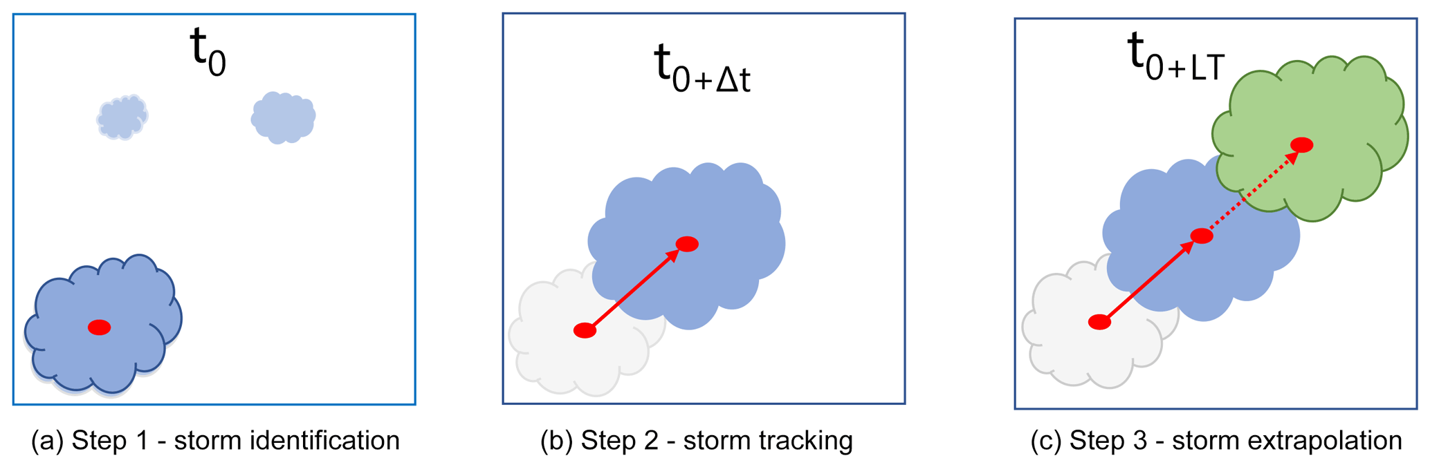
Figure 1 The main steps of an object-based radar nowcast. Blue indicates the current state of the storm at any time t, grey indicates the past states of the storm (at t₀+Δt), and green indicates the future states of the storm (t_0+LT) (Shehu, 2020).

Apart from the initialization errors mentioned before, other error sources in the object-based nowcast can be attributed to storm identification, storm tracking, and Lagrangian extrapolation (Foresti and Seed, 2015; Pierce et al., 2012; Rossi et al., 2015). Many works have already been conducted to investigate the role of different intensity thresholds in the storm identification or of different storm-tracking algorithms in the nowcasting results (Goudenhoofdt and Delobbe, 2013; Han et al., 2009; Hou and Wang, 2017; Jung and Lee, 2015; Kober and Tafferner, 2009). Very-high-intensity thresholds may be suitable for convective storms but can cause false splitting of the storms and can affect negatively the tracking algorithm. Thus, one has to be careful when adjusting the intensity threshold dynamically over the radar field and type of storm. A storm-tracking algorithm can be improved if certain relationships are learned from past observed datasets (like a fuzzy approach in Jung and Lee, 2015, or a tree-based structure in Hou and Wang, 2017), but there is still a limit that the tracking improvement cannot surpass due to the implementation of the Lagrangian persistence (Hou and Wang, 2017). These errors due to the Lagrangian persistence are particularly high for convective events at longer lead times (past 1 h) as the majority of convective storms dissipate within 60 min (Goudenhoofdt and Delobbe, 2013; Wilson et al., 1998). At these lead times, the persistence fails to predict the dissipation of these storm cells, while for shorter lead times it fails to represent the growing/decaying rate and the changing movement of a storm cell (Germann et al., 2006). For stratiform events, since they are more persistent in nature, Lagrangian persistence can give reliable results up to 2 or 3 h lead time (Krämer, 2008). Nevertheless, studies have found that, for fine spatial (1 km²) and temporal (5 min) scales, the Lagrangian persistence can yield reliable results up to 20–30 min lead time, which is also known in the literature as the predictability limit of rainfall at such scales (Grecu and Krajewski, 2000; Kato et al., 2017; Ruzanski et al., 2011). In object-based radar nowcasting, this predictability limit can be extended up to 1 h for stratiform events and up to 30–45 min for convective events if a better radar product (merged with rain-gauge data) is fed into the nowcast model (Shehu and Haberlandt, 2021). Past these lead times, the errors due to the growth/decay and dissipation of the storms dominate.

The predictability of convective storms can be extended if, instead of the Lagrangian persistence, one estimates these non-linear processes (growth/decay/dissipation) by utilizing storm life characteristics analysed from past observations (Goudenhoofdt and Delobbe, 2013; Zawadzki, 1973). For instance, Kyznarová and Novák (2009) used the CellTrack algorithm to derive life cycle characteristics of convective storms and observed that there is a dependency between storm area, maximum intensity, life phase, and height of the 0 ^∘C isotherm level. Similar results were also found by Moseley et al. (2013), who concluded that convective storms show a clear life cycle with the peak occurring at one-third of total storm life, a strong dependency on the temperature, and increasing average intensity with longer durations. In the case of extreme convective storms, earlier peaks are more obvious, causing a steeper increase to maximum intensity. A later study by Moseley et al. (2019) found that the longest and most intense storms were expected in the late afternoon hours in Germany. Thus, it is to be expected that an extensive observation of past storm behaviours can be very useful in creating and establishing new nowcasting rules (Wilson et al., 2010) that can outperform the Lagrangian persistence. An implementation of such learning from previous observed storms (with focus only on the object-based nowcast and not the field-based one) is for instance shown by Hou and Wang (2017), where a fuzzy classification scheme was implemented to improve the tracking and matching of storms, which resulted in an improved nowcast, and Zahraei et al. (2013), where a self-organizing-map (SOM) algorithm was used to predict the initialization and dissipation of storms at coarse scales, extending the predictability of storms by 20 %. These studies suggest that past observed relationships may be useful in extending the predictability limit of the convective storms. In this context, a k nearest-neighbour method (k-NN) may be developed at the storm scale and used to first recognize similar storms in the past and then assign their behaviours to the “to-be-nowcasted” storm. The nearest-neighbour method has been used in the field of hydrology, mainly for classification, regression, or resampling purposes (e.g. Lall and Sharma, 1996), but there are some examples of prediction as well (Galeati, 1990). The assumption of this method is that similar events are described by similar predictors, and if one identifies the predictors successfully, similar events that behave similarly can be identified. For a new event, the respective response is then obtained by averaging the responses of past k – the most similar storms. The k value can be optimized by minimizing a given cost function. Because of the averaging, the response obtained will be a new one, thus satisfying the condition that nature does not repeat itself, but nevertheless it is confined within the limits of the observed events (and therefore is unable to predict extreme behaviours outside of the observed range).

Similar approaches are implemented in field-based nowcast (referred to as analogue events), where past similar radar fields are selected based on weather conditions and radar characteristics, i.e. in the NORA nowcast by Panziera et al. (2011) mainly for orographic rainfall or in the multi-scaled analogue nowcast model by Zou et al. (2020). Panziera et al. (2011) showed that there is a strong dependency between air-mass stability, wind speed and direction, and the rainfall patterns observed from the radar data and that the NORA nowcast can improve the hourly nowcasts of orographic rain up to 1 h when compared to Eulerian persistence and up to 4 h when compared to the COSMO2 NWP. Improvement of predictability through a multi-scaled analogue nowcast was also reported by Zou et al. (2020), which identified neighbours first by accounting for similar meteorological conditions and then the spatial information from radar data. However, both of these studies show the applicability of the method to rainfall types that tend to repeat the rainfall patterns, i.e. the orographic forcing in the case of Panziera et al. (2011) and winter stratiform events in the case of Zou et al. (2020). So far, to the authors' knowledge, such application of the k-NN has not been applied for convective events. This application seems reasonable as an extension of the object-based radar nowcast in order to treat each convective storm independently. It can be used instead of the Lagrangian persistence in step 3 in Fig. 1c for the extrapolation of rainfall storms into the future. Moreover, the benefit of the k-NN application is that one can either give a single or an ensemble nowcast; since k neighbours can be selected as similar to a storm at hand, a probability based on the similarity rank can be issued at each of the past storms, thus providing an ensemble of responses which are more preferred compared to the deterministic nowcast due to the high uncertainty associated with rainfall predictions at such fine scales (Germann and Zawadzki, 2004). Thus, it is the aim of this study to investigate the suitability of the k-NN application for substituting the Lagrangian persistence in the nowcasting of mainly convective events that have the potential to cause urban pluvial floods.

We would like to achieve this by first investigating whether a k-NN is able to nowcast successfully storm characteristics like area, intensity, movement, and total lifetime for different life cycles and lead times. Based on the observed dependency of the storm characteristics on the life cycle, it would be interesting to see whether the morphological features are enough to describe the evolution of the convective storms. Therefore, the focus is here only on the features recognized by the radar data, and further works will also include the use of meteorological factors. To reach our aim, the suitability of the k-NN approach is studied as an extension of the existing object-based nowcast algorithm HyRaTrac developed by Krämer (2008). Before such an application, questions that arise are (I) which features are more important when describing a storm, (II) how to evaluate similarity between storms, and (III) how to use their information for nowcasting the storm at hand. The paper is organized as follows: first, in Sect. 2 the study area is described, followed by the structure of the k-NN method in Sect. 3.1, where the generation of the storm database is discussed in Sect. 3.1.1, the predictors selected and target variables in Sect. 3.1.2, the methods used for predictor identification in Sect. 3.1.3, and different applications of the k-NN in Sect. 3.1.4. The optimization and the performance criteria are shown in Sect. 3.2, followed by the results in Sect. 4 separated into predictor influence (Sect. 4.1), deterministic k-NN (Sect. 4.2), probabilistic k-NN performance (Sect. 4.3), and the nowcasting of unmatched storms (Sect. 4.4). Finally, the study is ended with conclusions and an outlook in Sect. 5.

2 Study area and data

The study area is located in northern Germany and lies within the Hanover Radar Range as illustrated in Fig. 2. The radar station is situated at Hanover Airport, and it covers an area with a radius of 115 km. The Hanover radar data are C-band data (single-polarization) provided by the German Weather Service (DWD) and measure the reflectivity at an azimuth angle of 1^∘ and at 5 min scans (Winterrath et al., 2012). The reflectivity is converted to intensity according to the Marshall–Palmer relationship with the coefficients a=256 and b=1.42 (Bartels et al., 2004). The radar data are corrected from the static clutters and erroneous beams and then converted to a Cartesian coordinate system (1 km² and 5 min) as described in Berndt et al. (2014), while the rain gauges measure the rainfall intensities at 1 min temporal resolution but are aggregated to 5 min time steps. Additionally, following the results from Shehu and Haberlandt (2021), a conditional merging between the radar data and 100 rain-gauge recordings (see Fig. 2b) with the radar range at 5 min time steps is performed. The conditional merging aims to improve the kriging interpolation of the gauge recordings by adding the spatial variability and maintaining the storm structures as recognized by the radar data. In case a radar image is missing, the kriging interpolation of the gauge recordings is taken instead.

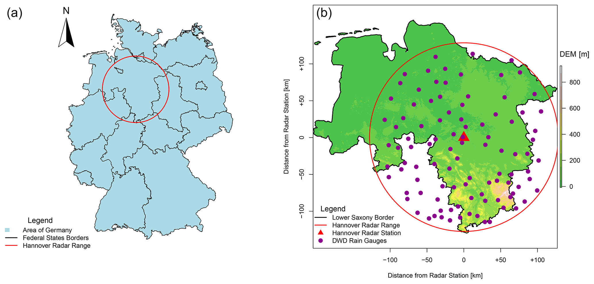
Figure 2 The location of the study area (a) within Germany and (b) with the corresponding elevation and boundaries and with the available recording rain gauges (purple) and radar station (red). “DEM” is short for “digital elevation model” (adapted from Shehu and Haberlandt, 2021).

The period from 2000 to 2018 is used as a basis for this investigation, from which 110 events with different characteristics were extracted (see Shehu and Haberlandt, 2021, or Shehu, 2020). These events were selected for urban flood purposes and contain mainly convective events and few stratiform ones. Here, rainfall events refer to a time period when rainfall has been observed inside the radar range and at least one rain gauge has registered an extreme rainfall volume (return period higher than 5 years) for durations varying from 5 min to 1 d. The start and the end of the rainfall event are determined when areal mean radar intensity is higher/lower than 0.05 mm for more than 4 h. Within a rainfall event many rainfall storms, at different times and locations, can be recognized. Figure 3a shows a simple illustration to distinguish between the rainfall event and rainfall storm concepts employed in this study.

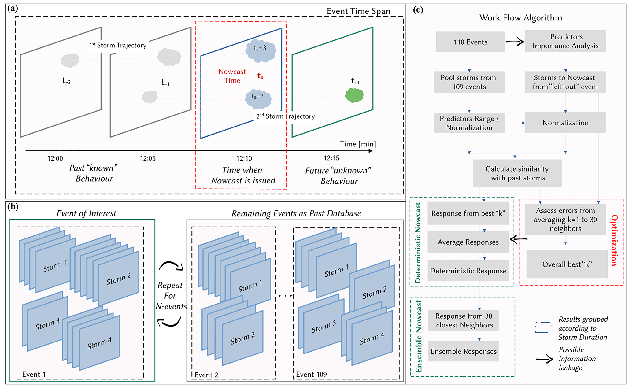
Figure 3 Illustration of concepts and workflows in this study. (a) An event contains many rainfall storms inside the radar range which are tracked and nowcasted: the dashed grey lines indicate the movements of storms in space and time within the radar event and the event time span. (b) The “leave-one-out-event cross-validation” – the storms of the event of interest are removed from the past database, and the nowcast of these storms is issued based on the past database. This process is repeated 110 times (once for each event). (c) The workflow implemented here for the optimization and application of the k-NN approach.

3 Methods

3.1 Developing the k-NN model

3.1.1 Generating the storm database

Each of the selected events contains many storms, whose identification and tracking were performed on the basis of the HyRaTrac algorithm in the hindcast mode (Krämer, 2008; Schellart et al., 2014). A storm is initialized if a group of spatially connected radar grid cells (>64) has a reflectivity higher than Z=20 dBz, while storms are recognized as convective if a group of bigger than 16 radar grid cells has an intensity higher than 25 dBz and as stratiform if a group of bigger than 128 radar grid cells has an intensity higher than 20 dBz. Typically, higher values (40 dBz) are used to identify the core of convective storms (as in E-Titan), but to avoid false splitting of convective storms and to test the methodology on all types of storms, these identification thresholds were kept low (also following the study of Moseley et al., 2013). Once storms at different time steps are recognized, they are matched as the evolution of a single storm if the centre of intensity of a storm at t=0 falls within the boundary box of the storm at t−5 min. The tracking of individual storms in consecutive images is done by the cross-correlation optimization between the last two images (t=0 and t−5 min), and local displacement vectors for each storm are calculated. In case a storm is just recognized (the storm does not yet have a previous history), then global displacement vectors based on cross-correlation of the entire radar image are assigned to them. It is usually the case that two storms merge together at a certain time or that a single storm splits between several daughter storms. The splitting and merging of the storms is considered here if two criteria are met: (a) the minimum distance between the storms that have split or merged is smaller than the perimeter of the merged or currently splitting storm and (b) the position of the centre of intensity of former/latter storms is within the boundaries of the latter/former storm.

Thus, a dataset with several types of storms is built and saved. The storms are saved with an ID based on the starting time and location, and for each time step of the storm evolution the spatial information is saved and various features are calculated. Here the features computed from the spatial information of the rainfall inside the storm boundaries at a given time step (in 5 min) of a storm's life are referred to as the “state” of the storm. A storm that has been observed for 15 min consists of three “states”, each occurring at a 5 min time step. For each of the storm states an ellipsoid is fitted to the intensities in order to calculate the major and minor axes and the orientation angle of the major axis. This storm database is the basis for developing the k-NN method and for investigating the similarity between storms. Some characteristics of the identified storms, like duration (or also total lifetime of the storm), mean area, maximum intensity, number of splits/merges, local velocity components, and ellipsoidal features, are shown in Fig. 4. These storm characteristics were obtained by a hindcast analysis run of all 110 events with the HyRaTrac algorithm, which resulted in around 5200 storms. The local velocities in the x and y directions are obtained by a cross-correlation optimization within the storm boundary. The life of the storm is then the lifetime of the radar pixel group as dictated by the threshold used to recognize them and the tracking algorithm that decides whether the same storm is observed at continuous time steps. For more information about the tracking and identification algorithm, the reader is directed to Krämer (2008).

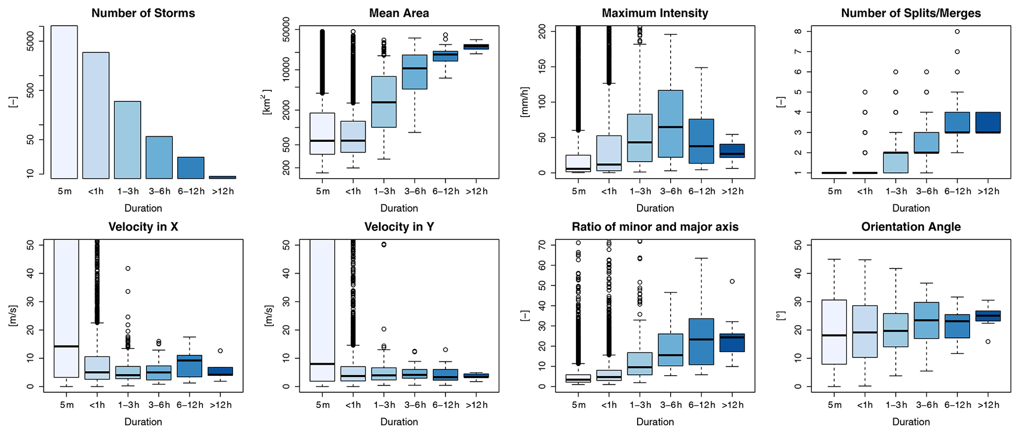
Figure 4 Different properties of the storms recognized from 110 events separated into six groups according to their duration (shown in different shades of blue).

As seen from the number of storms for each duration in Fig. 4, the unmatched storm cells make up the majority of the storms recognized. These are storms that last just 5 min (one time step), as the algorithm fails to track them at consecutive time steps. These “storms” can either be dynamic clutter from the radar measurement, as they are characterized by small areas, circular shapes (small ratios of minor and major axes), and very high velocities, or artefacts created by low-intensity thresholds used for the storm identification, or finally produced by the non-representativeness of the volume captured by the radar station. Another thing to keep in mind is that merged radars are fed to the algorithm for storm recognition, and this affects the storm structures, particularly when the radar data are missing. In such a case, the ordinary kriging interpolation of rain gauges is given as the input, which is well known to smoothen the spatial distribution of rainfall and hence result in a short storm characterized by a very large area. Since the unmatched storms can either be dynamic clutter or artefacts, they are left outside of the k-NN application. Nonetheless, they are treated briefly in Sect. 4.5.

Apart from the unmatched storms, the majority of the remaining storms are of a convective nature: storms with short duration (shorter than 6 h), high intensity, and low areal coverage. Here two types of convective storms are distinguished: local convective, with very low coverage (on average lower than 1000 km²) and low intensity (on average ∼5 mm h⁻¹), and mesoscale convective, which are responsible for floods (with intensity up to 100 mm h⁻¹ or more) and have a larger coverage (on average lower than 5000 km²). The stratiform storms characterized by large areas, long durations, and low intensities as well as meso-γ-scale convective events with durations of up to 6 h are not very well represented by the dataset, as only a few of them are present in the selected events (circa 20 and 50 storms respectively). Therefore, it is to be expected that the k-NN approach will not yield very good results for such storms due to the low representativeness. From the characteristics of the storms illustrated in Fig. 4, it can be seen that for stratiform storms that last longer than 12 h the variance of the characteristics is quite low (when compared to the rest of the storms), which can be attributed either to the persistence of such storms or to the low representativeness in the database. Even though the data size for stratiform storms is quite small, the k-NN may still deliver good results as characteristics of such storms are more similar. Nevertheless, the stratiform storms are typically nowcasted well by the Lagrangian persistence (especially by a field-oriented approach), as they are widespread and persistent. Hence the value of the k-NN is primarily seen for convective storms and not for stratiform ones.

3.1.2 Selecting features for similarity and target variables

At first storms are treated like objects that manifest certain features (predictors) like area, intensity, or lifetime at each state of a storm's duration until the storm dissipates (and the predictors are all set to zero). The features of the objects are categorized into present and past features, as illustrated in Fig. 5 (shown respectively in blue and grey). The present features describe the current state of the storm at the time of nowcast (denoted with t₀ in Fig. 5) and are calculated from one state of the storm. To compute certain features, an ellipsoid is fitted to each state of the storm. The past features, on the other hand, describe the predictors of the past storm states (denoted with t₋₁, t₋₂ in Fig. 5) and their change over the past life of the storm. For example, the average area from times t₋₂ to t₋₁ is a past feature. A pre-analysis of important predictors showed that the average features over the last 30 min are more suitable as past predictors than the averages over the past 15 or 60 min or than the calculation of past changing rates. Therefore, averages over the past 30 min are computed here:

$$\begin{array}{}\text{(1)}& P_{\mathrm{30}}={\sum }_{i=t_{\mathrm{0}}}^{t-\mathrm{30}\min }{P}_i/\mathrm{7},\end{array}$$

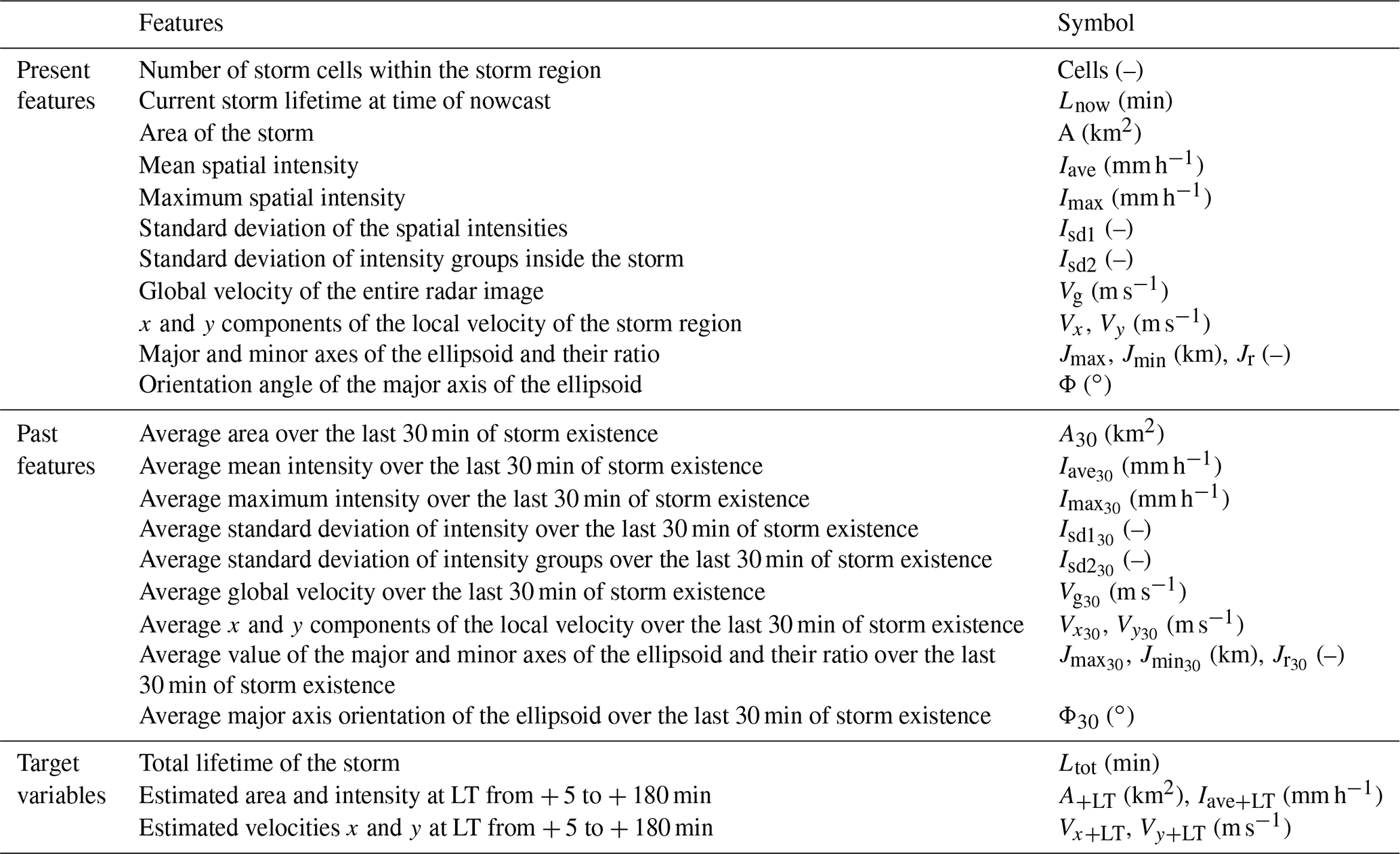
where P_i is the predictor value at time i and P₃₀ is the average value of the predictor over the last 30 min. In case of missing values, the remaining time steps are used for averaging. The selected features (both present and past) that are used here to describe storms as objects, and hence tested as predictors, are shown in Table 1. The present features help to recognize storms that are similar at the given state when the nowcast is issued (blue storm in Fig. 5), and the past ones give additional information about the past evolution of the storm (average of grey storms in Fig. 5). The aim of these features is to recognize the states of previously observed storms that are most similar to the current one (shown in blue in Fig. 5) of the to-be-nowcasted storm. Once the most similar past storm states are recognized, their respective future states at different lead times can be assigned as the future behaviour (shown in green in Fig. 5) of the current state of the to-be-nowcasted storms. Since the storms are regarded as objects with specific features, future behaviours at different lead times are determined by four target variables: area (A_+LT), mean intensity (I_+LT), and velocities in the x (V_x+LT) and y (V_y+LT) directions. Additionally, the total lifetime of the storm is considered a fifth target (L_tot). Theoretically, the total lifetime is predicted indirectly when any of the first four targets is set to zero; however, here it is considered an independent variable in order to investigate whether similar storms have similar lifetime durations.

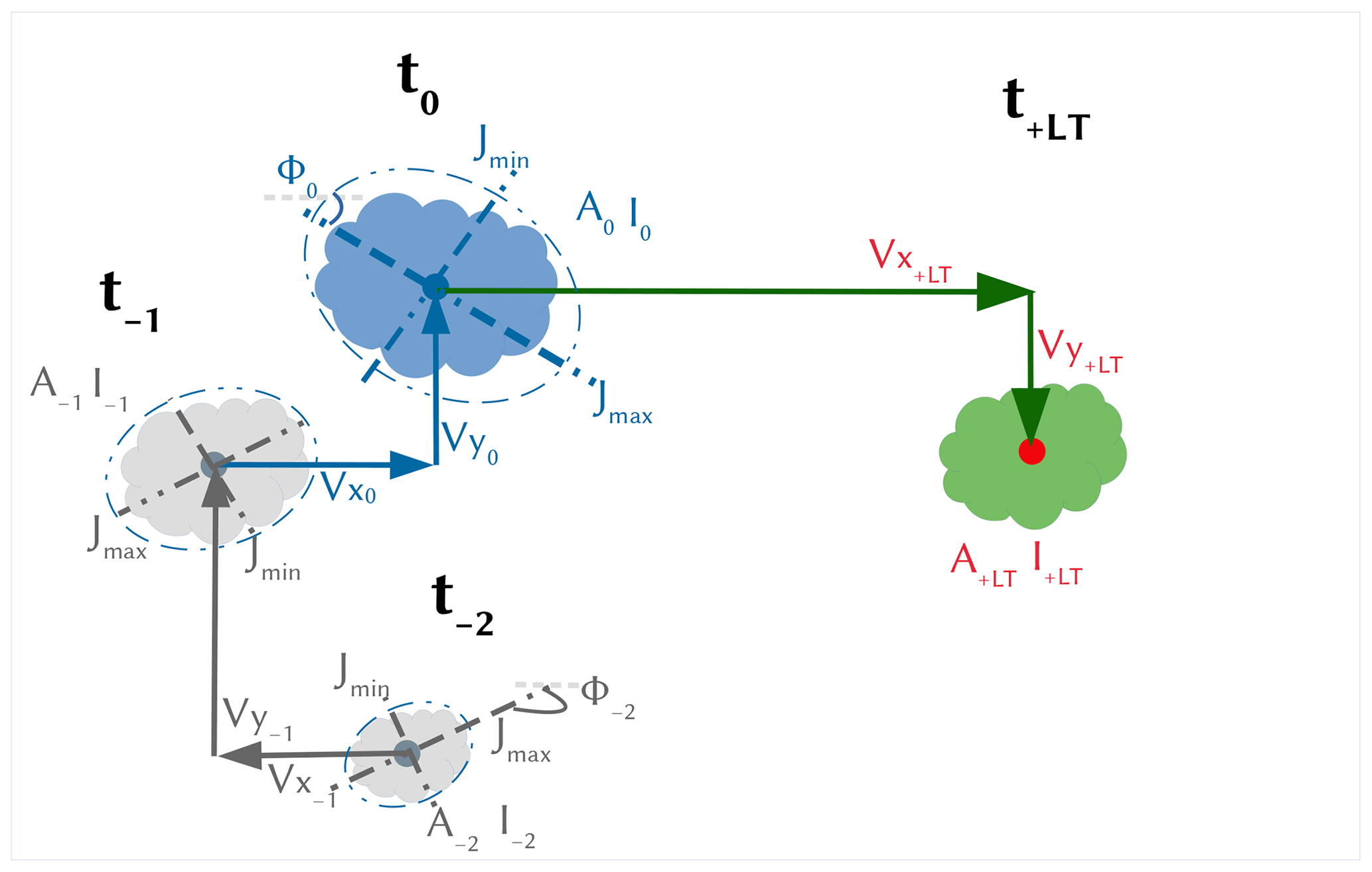
Figure 5 The features describing the past (grey) and present (blue) states of the storm used as predictors to nowcast the future states of the storm (green) at a specific lead time (T_+LT) that are described by four target variables (in red). The nowcast is issued at time t₀. A full description of these predictors and target variables is given in Table 1.

For each state of each observed storm in the database, the past and present features of that state with its respective future states of the five target variables from + 5 to + 180 min (every 5 min) lead times are saved together and form the predictor–target database that is used for the development of the k-NN nowcast model. A summary of the predictors and target variables calculated per state is given in Table 1. Before optimizing and validating the k-NN method (see Fig. 3c), an importance analysis is performed for each of the target variables in order to recognize the most important predictors. As the predictors have different ranges, prior to the importance analysis and the k-NN application, they are normalized according to their median and range between the 0.05 and 0.95 quantiles:

$$\begin{array}{}\text{(2)}& \mathrm{norm}{P}_i={\displaystyle \frac{P_i-Q_{P_i}^{\mathrm{0.5}}}{Q_{P_i}^{\mathrm{0.95}}-Q_{P_i}^{\mathrm{0.05}}}},\end{array}$$

where P is the actual value, normP the normalized value, and $Q_{P_i}^{\mathrm{0.5}}$, $Q_{P_i}^{\mathrm{0.95}}$, and $Q_{P_i}^{\mathrm{0.05}}$ the quantiles 0.5, 0.05, and 0.95 of the ith predictor vector. The reason why these quantiles were used for the normalization instead of the typical mean and maximum to minimum range is that some outliers are present in the data. For instance, very high and unrealistic velocities are present in some convective storms where the tracking algorithm fails to capture adequate velocities (Han et al., 2009). Thus, to avoid the influence of these outliers, the given range is employed.

3.1.3 Selection of the most relevant predictors

The application of the k-NN method can be relevant if there is a clear connection between the target variable and the features describing this target variable. For instance, in the case of Galeati (1990), a physical background backed up the connection between the target variable (discharge) and the features (daily rainfall volume and mean temperature). In the case of the storms at such fine temporal and spatial scales, due to the erratic nature of the rainfall itself, there is no physically related information that can be extracted from radar data. Different features of the storm itself can be investigated for their importance to the target variable. Nevertheless, the identification of such features (referred to here as predictors) is difficult because it is bounded to the set of the available data and the relationships considered. Commonly a strong Pearson correlation between the predictors selected and the target variable is used as an indicator of a strong linear relationship between them. Here, the Pearson correlation absolute values are used directly as predictor weights in the k-NN application. However, the relationship between predictors and target variables may still be of a non-linear nature, and thus another predictor importance analysis should be recommended when selecting the predictors. Sharma and Mehrotra (2014) proposed a new methodology, designed specifically for the k-NN approach, where no prior assumption about the system type is required. The method is based on a metric called the partial information correlation and is computed from the partial information as

$$\begin{array}{}\text{(3)}& \begin{array}{rl}& \mathrm{PIC}=\sqrt{(\mathrm{1}-\exp (-\mathrm{2}\mathrm{PI})}\mathrm{with}\mathrm{PI}=\int f_{x,P\mathrm{|}Z}\left(x,p|z\right)\\ & \log \left[{\displaystyle \frac{f_{x\left|Z,P\right|Z}\left(x,p|z\right)}{f_{x\mathrm{|}Z}\left(x|z\right)f_{P|Z}\left(p|z\right)}}\right]\mathrm{d}x\mathrm{d}p\mathrm{d}z,\end{array}\end{array}$$

where PIC is the partial information correlation and PI is the partial information which represents the partial dependence of x on P conditioned to the presence of a predictor Z. The partial information itself is a modification of the mutual information in order to measure partial statistical dependency between the predictors (P) and the target variable (x) by adding predictors one at a time (Z) (step-wise procedure). The evaluation of the PIC needs a pre-existing identified predictor from which the computation can start. If the pre-defined predictor is correctly selected, then, through Eq. (3), the method is able to recognize and leave out the new predictors which are not related to the response and which do not bring additional value to the existing relationship between the current predictors and target variable. Relative weights for the k-NN regression application can be derived for each predictor as a relationship between the PIC metric and the associated partial correlation:

$$\begin{array}{}\text{(4)}& {\mathit{\alpha }}_j={\mathrm{PIC}}_{x,Zj\left|Z\right(-j)}{\displaystyle \frac{S_{x\left|Z\right(-j)}}{S_{Zj\left|Z\right(-j)}}},\end{array}$$

where x is the target response, Zj is the added predictor from the step-wise procedure, Z(−j) is the previous predictor vector excluding the predictor Zj, $S_{x\left|Z\right(-j)}$ are the scaled conditional standard deviations between the target (x) and predictor vector Z(−j), $S_{Zj\left|Z\right(-j)}$ are the scaled conditional standard deviations between the additional predictor (Zj) and the first predictor vector Z(−j), and α_j is the predictor weight. R package NPRED was used for the investigation of the PIC-derived importance weights (Sharma et al., 2016).

Here, in this study, these two importance analyses are used to determine the most important predictors and their respective weights in the k-NN similarity calculation. For each target variable the most important predictor identified from Pearson correlation is given to the PIC metric as the first predictor. The analysis is complex due to the presence of several predictors, 38 states of future behaviour for each target variable (for every 5 min between + 5 and + 180 min lead times), and different nowcast times; the weights were calculated first for three lead times + 15, + 60, and + 180 min and for three storm groups separated according to their durations <60 min, 60–180 min, and >3 h. Here the average weights over these groups and lead times are calculated and used as a reference for each importance analysis. The k-NN errors with these average weights are compared in Sect. 4.1.

Table 1 List of all the past and present features of the storms that are investigated for their importance as predictors, and the respective target variables calculated for different lead times.

3.1.4 Developing the k-NN structure

The structure of the proposed k-NN approach at the storm scale is illustrated in Fig. 6 – the current to-be-nowcasted storm is shown on the left and the past observed storms on the right. First, in step 1, the Euclidean distance between the most important predictors (either present or past predictors) of past storm states and the current one is calculated to identify the most similar states of the past storms (distance between the blue shapes on the left- and right-hand sides of Fig. 6):

$$\begin{array}{}\text{(5)}& E_{\mathrm{d}}=\sqrt{{\sum }_{i=\mathrm{1}}^N{w}_i\cdot {\left(x_i-y_i\right)}^{\mathrm{2}}},\end{array}$$

where w is the weight of the respective ith predictor as dictated by the importance analysis (results are shown in Table 3), x is the predictor of the to-be-nowcasted storm, y is the predictor of a past observed storm, N is the total number of predictors used, and E_d is the Euclidian distance between the to-be-nowcasted and past observed storms. The assumption made here is that the smaller the distance, the higher the similarity of future behaviour between the selected storms and the to-be-nowcasted storm. Therefore, in step 2 these distances are ranked in ascending order and 30 past storm states with the smallest distance are selected (step 3). Once the similar past storm states have been recognized (the blue shape in Fig. 6 – right), the future states of these storms (the green shapes in Fig. 6 – right, each for a specific lead time from the occurrence of the selected similar blue state) are treated as future states (the green shape in Fig. 6 – left) of the to-be-nowcasted storm. In step 4, either a single (deterministic) or an ensemble (probabilistic) nowcast is issued. If a single nowcast is selected, then the green instances of the k neighbours are averaged with weights for each lead time:

$$\begin{array}{}\text{(6)}& R_{\mathrm{new}}={\sum }_{i=\mathrm{1}}^k{\mathrm{Pr}}_i\cdot R_i,\end{array}$$

where k is the number of neighbours obtained from optimization, R_i and Pr_i (from Eq. 7) are respectively the response and weight of the ith neighbour, and R_new is the response of the to-be-nowcasted storm as averaged from k neighbours. The response R refers to each of the five target variables: area, intensity, velocities in the x and y directions, and total lifetime. By contrast, if a probabilistic nowcast is selected, 30-member ensembles are selected from the closest 30 storms, where each member is assigned a probability according to the rank of the respective neighbour storm:

$$\begin{array}{}\text{(7)}& {\mathrm{Pr}}_i={\displaystyle \frac{(\mathrm{1}/{\mathrm{Rank}}_i)}{{\sum }_{i=\mathrm{1}}^k(\mathrm{1}/{\mathrm{Rank}}_i)}},\end{array}$$

where k is the selected number of neighbours and Rank and Pr are respectively the rank and the probability weights of the i neighbour $/$ ensemble member. An ensemble member is then selected randomly based on the given probability weights. These probability weights calculated here are also used for computation of the single nowcast in Eq. (6).

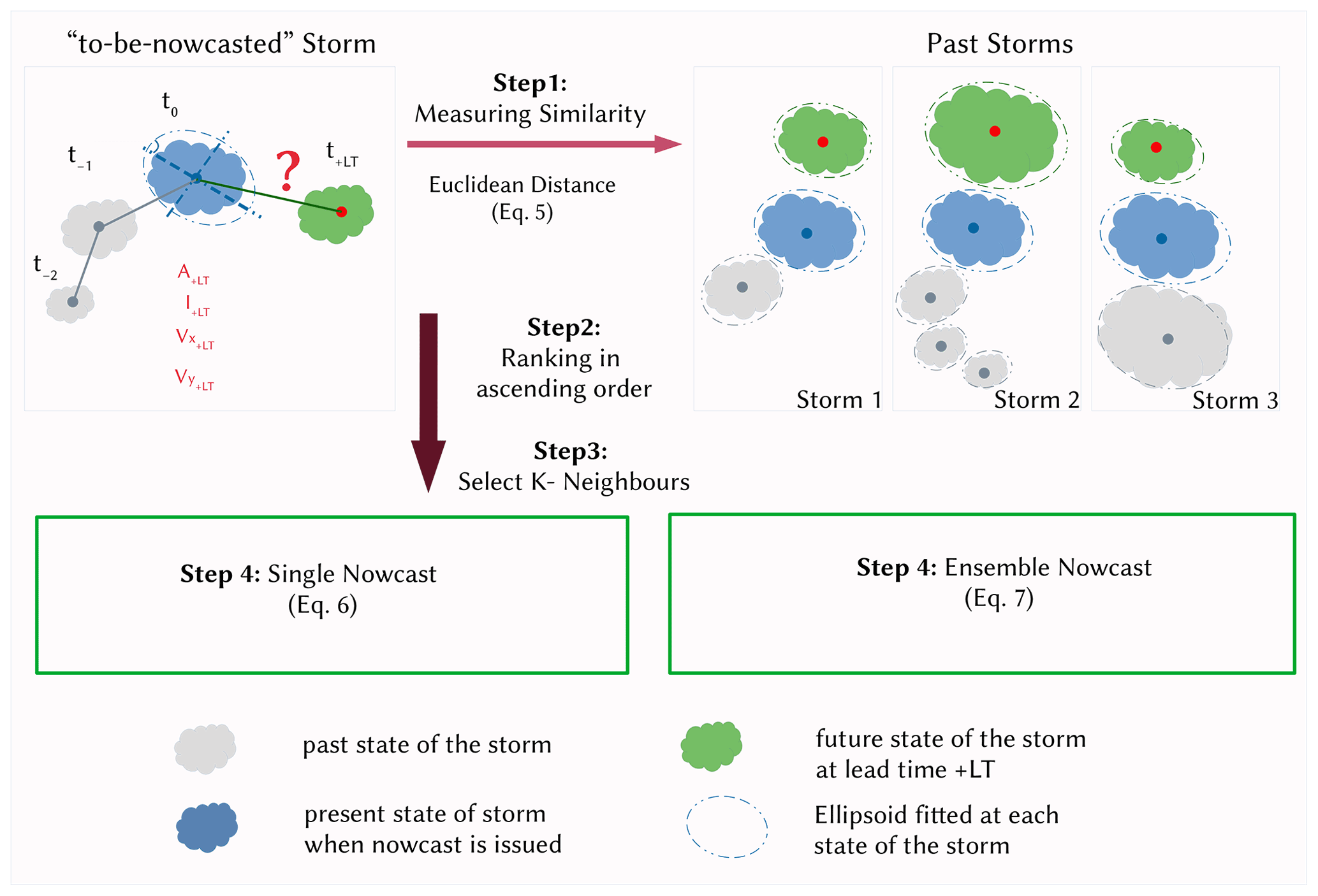
Figure 6 The main steps involved in the k-NN-based nowcast with the estimation of similar storms (Steps 1 to 3) and assigning the future responses of past storms as the new response of the “to-be-nowcasted” storm either in a deterministic nowcast (Step 4 – left) or in a probabilistic nowcast (Step 4 – right).

Since the performance of the single k-NN nowcast is highly dependent on the number of k neighbours used for the averaging, a prior optimization should be done in order to select the right k neighbours that yield the best performance (as illustrated in Fig. 3c). The application of the k-NN can either be done for each target variable independently or for all target variables grouped together. In the first approach, the dependency of the target variables between one another is not assured: they are predicted independently of one another. This is referred to here as the target-based k-NN and is denoted in the results as VS1. The main advantage of this application is that, since the relationships between the target variables are not kept, new storms can be generated. Theoretically, the predicted variables should have a lower error since the application is done separately for each variable; nevertheless, this approach does not say much about whether similar storms behave similarly. Therefore, it is used here as a benchmark for the best possible optimization that can be reached by the k-NN with the current selected predictor set. In the second approach, the relationships between target variables as exhibited by previous storms are kept. The storm structure and the relationship between features are maintained as observed, and thus the question of whether similar storms behave similarly can be answered. This is referred to here as the storm-based k-NN and is denoted in the results as VS2. In this study the two approaches are used (respectively called VS1 and VS2) to understand the potential and the actual improvement that the k-NN can bring to the storm nowcast.

3.2 Application of the k-NN and performance assessment

3.2.1 Optimizing the deterministic k-NN nowcast

The optimization of the k-NN is done based on the 5189 storms extracted from 110 events in a “leave-one-out” cross-validation. Since the unmatched storms can be either dynamic clutter or artefacts of the tracking algorithm, they are left outside of the k-NN optimization and validation. The assumption is here that an improvement of the radar data or tracking algorithm would eliminate the unmatched storms, and hence the focus is only on the improvement that the k-NN can introduce to the matched storms. “Leave-one-event-out” cross-validation means here that the storms of each event have to be nowcasted by considering as a past database the storms from the remaining 109 events (a detailed visualization is given in Fig. 3b). The objective function is the minimization of the mean absolute error (MAE) (Eq. 8) and of the absolute mean error (ME) (Eq. 9) between predicted and observed target variables at lead times from + 5 to + 180 min:

$$\begin{array}{}\text{(8)}& {\displaystyle }{\mathrm{MAE}}_{\mathrm{target}}={\sum }_{i=\mathrm{1}}^N\left(\right|{\mathrm{Pred}}_{i,+\mathrm{LT}}-{\mathrm{Obs}}_{i,+\mathrm{LT}}\left|\right)/N,\text{(9)}& {\displaystyle }{\mathrm{ME}}_{\mathrm{target}}=\left|{\sum }_{i=\mathrm{1}}^N({\mathrm{Pred}}_{i,+\mathrm{LT}}-{\mathrm{Obs}}_{i,+\mathrm{LT}})/N\right|,\end{array}$$

where Pred is the predicted response, Obs the observed response for the ith storm, +LT the lead time, and N the number of storms considered inside an event. The results of the storms' nowcast are also dependent on the nowcast time with respect to the storms' life (time step of the storm existence when the nowcast is issued – refer to Fig. 3a). If the nowcast time is 5 min, only the present predictors are used for the calculation of storm similarity and as higher nowcast time as more predictors are available for the similarity calculation. It is expected that the nowcast will perform worse in the first 5 min of the storm's existence, as the velocities are not assigned properly to the storm region and the past predictors are not yet calculated. Therefore, the optimization is done separately for three different groups of nowcast times in order to achieve a proper application of the k-NN model: Group 1 – nowcast issued at the first time step of storm recognition, Group 2 – nowcast issued between 30 min and 1 h of storm evolution, and Group 3 – nowcast issued between 2 and 3 h of storm evolution. The k number with the lowest absolute error averaged over all the events for most of the lead times (as the median of MAE from Eq. 9 and ME from Eq. 9 over all events) is selected as a representative for the deterministic nowcast.

3.2.2 Validating the k-NN deterministic and probabilistic nowcasts

Once the important predictors are identified and the k-NN has been optimized, the performance of both deterministic and probabilistic k-NN is also assessed in a leave-one-event-out cross-validation mode. Two performance criteria are used to assess the performance.

• i

  Absolute error per lead time and target variable computed for each event and a specific selected nowcast time:

  $$\begin{array}{}\text{(10)}& {\mathrm{MAE}}_{\mathrm{target}}={\sum }_{i=\mathrm{1}}^N\left(\right|{\mathrm{Pred}}_{i,+\mathrm{LT}}-{\mathrm{Obs}}_{i,+\mathrm{LT}}\left|\right)/N,\end{array}$$

  where Pred is the predicted response, Obs is the observed response for the ith storm, +LT is the lead time, and N is the number of storms considered inside an event.

• ii

  The improvement (%) for each lead time and target variable that the k-NN approach introduces to the nowcast (for a specific selected nowcast time) when compared to the Lagrangian persistence in an object-based approach:

$$\begin{array}{}\text{(11)}& {\mathrm{Error}}_{\mathrm{impr}}\left[\mathit{\%}\right]=\mathrm{100}\cdot {\displaystyle \frac{\left(\left|{\mathrm{Error}}_{\mathrm{ref}}\right|-\left|{\mathrm{Error}}_{\mathrm{new}}\right|\right)}{\left|{\mathrm{Error}}_{\mathrm{ref}}\right|}},\end{array}$$

where​​​​​​​ Error_new is the event error manifested by the k-NN, Error_ref is the event error manifested by the Lagrangian persistence, and Error_impr is the improvement in reducing the error for each lead time. For improvements higher than 100 % or lower than −100 %, the values are reassigned to the limits 100 % and −100 % respectively. Here the Lagrangian persistence refers to a persistence of the storm characteristics (area, intensity, and velocities in the x and y directions) as last observed and constant for all lead times.

For the probabilistic approach, the continuous rank probability score (CRPS) as shown in Eq. (12) is computed.

$$\begin{array}{}\text{(12)}& \begin{array}{rl}\mathrm{CRPS}\left(F,y\right)& =\underset{-\mathrm{\infty }}{\overset{\mathrm{\infty }}{\int }}(F\left(x\right)-\mathrm{1}\left\{y\le x\right\}{)}^{\mathrm{2}}\mathrm{d}x\\ & =E_F\left|y-y\right|-{\displaystyle \frac{\mathrm{1}}{\mathrm{2}}}{E}_F\left|y-y^{\prime }\right|,\end{array}\end{array}$$

where F is a probabilistic forecast, y is the observed value, and y and y^′ are independent random variables with a cumulative distribution function (CDF) of F and finite first moment E (Gneiting and Katzfuss, 2014). The CRPS is a generalization of the mean absolute error, and thus if a single nowcast is given, it is reduced to the mean absolute error (Eq. 10). This enables a direct comparison between the probabilistic and deterministic nowcasts and an investigation of the advantages of the probabilistic one. As in Eq. (8), the values obtained in Eqs. (10), (11), and (12) are averaged for each of the 110 events.

As stated earlier, the results depend on the nowcast time and also storm duration (with regard to available storms). Therefore, the performance criteria for both k-NN nowcasts were computed separately for different storm durations and nowcast times as illustrated in Table 2. It is important to mention as well that since one event may contain many storms of a similar nature, when leaving one event out for the cross-validation, the number of available storms is actually lower than the numbers given in Table 2. This particularly affects the performance of the storms longer than 6 h, as the leave-one-event-out cross-validation leaves fewer available storms for the similarity computation. Lastly, it is important to notice that the performance criteria can be calculated even for nowcast times longer than the storm lifetime if the nowcast fails to capture the dissipation of the storms. In this case, area, intensity, and velocity in the x and y directions are compared against zero and the total lifetime against the total observed lifetime of the storms.

Table 2 The selected storm durations and nowcast times for the performance calculation of the deterministic and probabilistic nowcasts and the respective number of storms for each case.

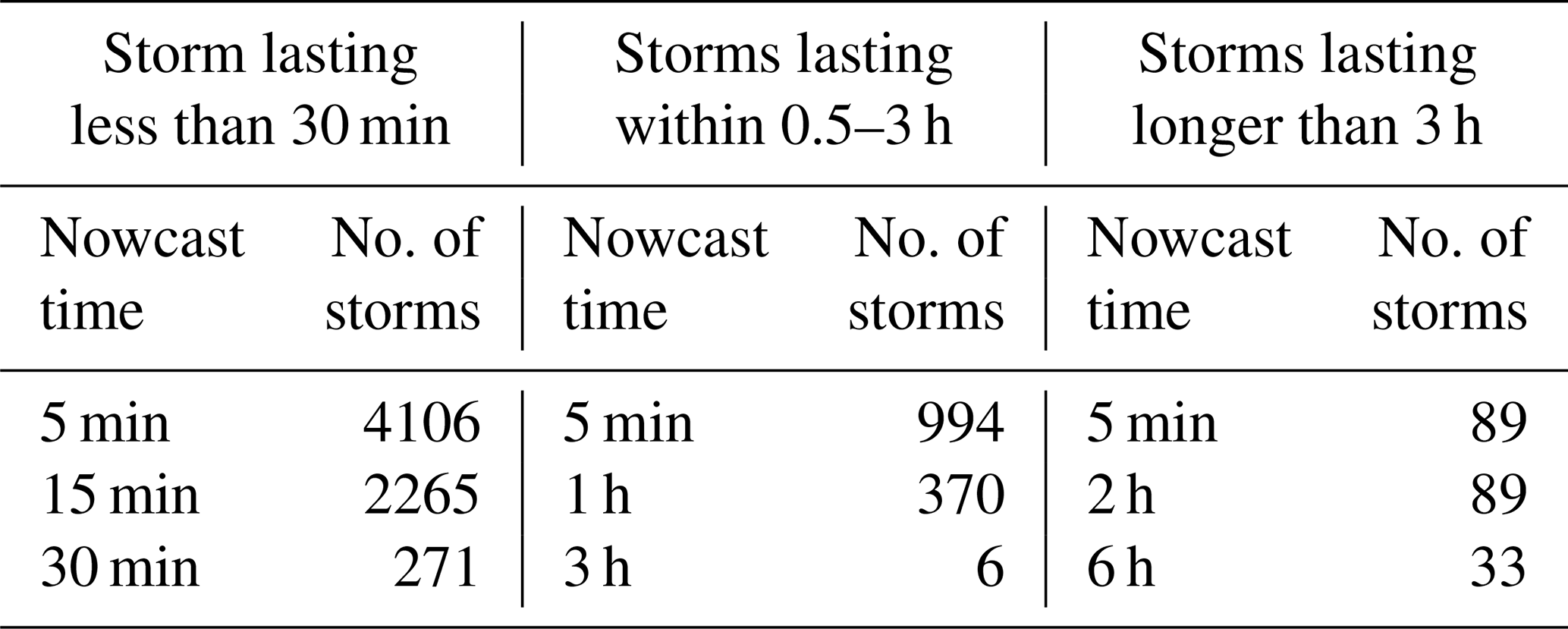
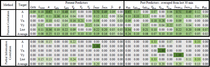
Table 3 Strength of the relationship between the selected predictors and the target variables averaged for three lead times and storm duration groups (original weights can be seen in Appendices 11.1 and 11.2) based on two predictor identification methods: upper – correlation – and lower – PIC weights. The green shade indicates the strength of the relationship, with 0 for no relationship at all and 1 for the highest dependency.

4 Results

4.1 Predictor importance analysis

Table 3 illustrates the results of the two importance analysis methods (Pearson correlation and PIC) for each of the target variables and their average over the five variables. The stronger the shade of the green colour, the more important is the predictor for the target variable. The weights given here are averaged from the weights calculated at three different lead times and storm durations (see Appendices 11.1 and 11.2 for more detailed information about the calculated weights). First the Pearson correlation weights are recommended for the identification of the most important predictors. From the results it is clear that the autocorrelation has a higher influence, as the target variables are mostly correlated with their respective past and present values. This influence logically is higher for the shorter lead times and smaller for the longer lead times. For longer lead times the importance increases of other predictors that are not related directly to the target variable. Similar patterns can be observed among the area, intensity, and total lifetime target variables, indicating that these three variables may be dependent on each other and on similar predictors like current lifetime, area, standard deviation of intensity, the major and minor ellipsoidal axes, and the global velocity. This conclusion agrees well with the life cycle characteristics of convective storms reported in the literature review. On the other hand are the velocity components, which seem to be highly dependent on the autocorrelation and slightly correlated with area and the ellipsoidal axes. It has to be mentioned that, apart from the standard deviation intensities, also the mean, median, and maximum spatial intensities were investigated. Nevertheless, it was found that the I_sd1 and I_sd2 had the higher correlation weights, and since there is a high collinearity between these intensity predictors, they were left out of the predictor's importance analysis.

The application of the PIC analyses requires that the most important predictors should be introduced to the analysis first. Hence, based on the Pearson correlation values from Table 3, the following most important predictors were selected: area – A (as the maximum correlation value from the first row), intensity – PI_sd1 (as the maximum correlation value from the second row), velocity x – Vx₃₀ (as the maximum correlation value from the third row), velocity y – Vy₃₀ (as the maximum correlation value from the fourth row), and total lifetime – A (as the maximum correlation value from the fifth row). The results of the PIC analysis are shown in the lower row of Table 3 and in Appendix 11.2. For storm duration lower than 3 h, where a lot of zeros are present, the PIC method seems to be unable to converge to stable results or to identify important predictors. For the intensity and velocity components, the PIC identifies only one important predictor, which, in the case of the intensity and velocity in the y direction, does not correspond to the most important predictor fed first in the analysis. In contrast, for total lifetime and area, only for storms that last longer than 3 h is the method able to converge and give the most important predictors: for area – A, Vg, past Vy₃₀, and L_now; for total lifetime – A, Vel_g, L_now, and Jmin₃₀. At the moment it is unclear why the PIC method is unable to perform well for all of the target variables and storm groups. One reason might be that only the area and total lifetime are dependent on the chosen target variables. Another most probable reason might be that for the other target variables the heavy tail of the probability distribution and the high zero sample size may influence the calculation of the joint and mutual probability distribution. The total lifetime is an easier target to be analysed, which means the values are not zero and its distribution is not as heavy tailed as the distribution of the other variables. The other variables, depending on the lead time, have more zeros included and have an asymptotic density function. It seems that, whenever zeros are not present, like in the case of storms lasting longer than 3 h, the PIC is able to represent quite well the important predictors. However, the reason why this method performs poorly for the application at hand, even though developed specifically for the k-NN application, is not completely understood and is not investigated further for the time being since it is outside the scope of this paper.

Overall, the results from the Pearson correlation seem more robust and stable (throughout the lead times and storm groups) than the PIC method (refer to Appendices 11.1 and 11.2); the importance weights increase with the lifetime of the storm and decrease with higher lead time. These behaviours are expected, as with increasing lead time the uncertainty becomes bigger and with increasing lifetime the storm dynamic becomes more persistent (due to the large scales and the stratiform movements involved). Moreover, the important predictors do not change drastically from one lead time or storm group to the other, as seen in the PIC. Therefore, the predictors estimated from the correlation with the given weights in Table 3 are used as input to the k-NN application. In order to make sure that the predictor set from the Pearson correlation was the right one, the improvement in the single k-NN training error of using these predictors instead of the ones from PIC are shown in Fig. 7. The results shown in this figure are computed according to Eq. (11) (where “new” is the k-NN with correlation weights and “ref” is the k-NN with PIC weights) for the target-based k-NN approach (solid lines) and storm-based k-NN approach (dashed lines) and are averaged for three groups of nowcast times as indicated in the optimization of the k-NN (Sect. 3.2.3) and in the legend of Fig. 7.

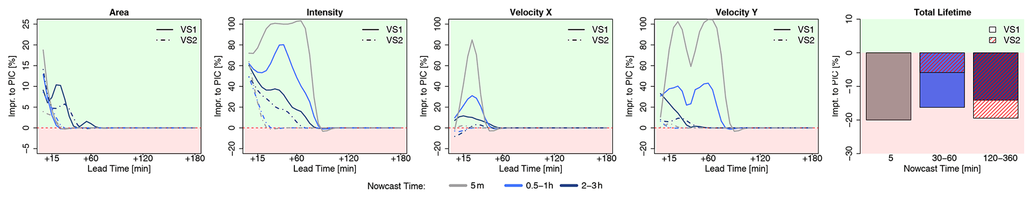
Figure 7 The median mean absolute error (MAE) improvement per lead time and target variable from applying the k-NN (VS1 target-based, VS2 storm-based) with the predictors and weights derived by the Pearson correlation instead of PIC. The improvements are averaged for different times of nowcast. The green plot region indicates a positive improvement of the correlation predictors in comparison to the PIC, and the red region indicates a deterioration.

The results from Fig. 7 indicate that, for the area, intensity, and velocity components, the Pearson correlation weights improve the performance of target-based k-NN from 5 % up to 100 % compared to the PIC weights. This happens mainly for the short lead times (LT <+60 min) throughout the three groups of nowcast times. For longer lead times there seems to be no significant difference between the predictor sets. The same cannot be said for the total lifetime as a target variable: here the Pearson correlation weights do not give the best results for all the nowcast times. In fact, here the k-NNs based on the PIC weights seem to be more appropriate and yielded better results. However, as the other four target variables are better for the Pearson correlation, this predictor set was selected for all applications of the k-NNs (with different weights according to Table 3) to keep the results consistent with one another. A further analysis was done that proved that the application of the correlation weights produces lower errors than the non-weighted k-NN application (all weights of the most important predictors from Pearson correlation are assigned as 1).

Lastly, it should be emphasized that, for the computation of predictor weights, all the events were grouped together, and thus when applying the k-NN nowcast in the cross-validation mode, there is a potential that the information will leak from the importance analysis to the performance of the k-NN (also illustrated in Fig. 3c). In other words, the performance of the k-NN will be better, because the weights were derived from all the events grouped together. Typically, in modelling applications, the optimization dataset should be clearly separated by the validating one in order to remove the effect of such information leakage. For this purpose, the correlation weights were computed 110 times, on a leave-one-event-out cross-sampling, in order to investigate their dependence on the event database. The results of such cross-sampling are visualized in Appendix 11.3 and indicate a very low deviation of the predictor weights (lower than 0.01) over all the target variables. The shown low variability of the Pearson correlation weights justifies the decision to estimate the weights from the whole database, as the potential information leakage likely does not affect the results of the k-NN performance. This is another reason favouring the calculation of the predictor's weights based on the Pearson correlation. On the other hand, the weights from the PIC analysis change very drastically depending on the dataset, and hence the effect of the information leakage would be much larger in the k-NN developed from PIC weights. Moreover, a sensitivity analysis as done in Appendix 11.3 cannot be performed for the PIC analysis because it would be extremely time-consuming.

4.2 Optimizing the deterministic k-NN nowcast

Once the most important predictors and their weights are determined, the optimization of the single k-NN nowcast for the two k-NN applications (storm-based and target-based) was performed. The optimal k values obtained from minimizing the MAE produced by k-NN are shown in Fig. 8, upper row. The results are computed for the given nowcast times, lead times, and target variables for both k-NN applications (VS1 target-based and VS2 storm-based). For the four target variables, area, intensity, and velocities in the x and y directions, the number of optimal values decreases quasi-exponentially for a lead time up to 1 h. After these lead times, when the majority of the storms are dissipated, the optimal k number converges at 1, meaning that the closest neighbour is enough to predict the dissipation of the storms. In contrast, for the very short lead times, the closest identified neighbour is unable to capture the growth/decay processes of the storms, and thus the response has to be the average from k neighbours, with k depending strongly on target variable, nowcast time, lead time, and total lifetime. This seems to be the case also for the total lifetime, where averages between 3 and 15 neighbours are computed as K_min. Overall, k=1 seems to yield the lowest MAE for the majority of the lead times, nowcast times, and target variables and therefore is selected to continue further with the analyses. However, selecting the first neighbour does not satisfy the requirement that nature does not repeat itself, and ideally k>1 should be achieved such that the responses from similar neighbours can be averaged to create a new response. For this purpose, the optimal K values were additionally obtained by minimizing the absolute ME and are shown in Fig. 8 – lower row. Here the overestimation and underestimation of different storms balance one another, and the results seem to converge when averaging three to five neighbours. A direct comparison of the MAE for k∼ 2–5 and k=1 was performed in order to understand whether a higher k will benefit the application of both k-NN versions. The median improvements of using neighbours from 2 to 5 instead of 1 (over the selected groups of nowcast times) are shown only for the total lifetime in Table 4. The other target variables are left outside this analysis as the improvements averaged over all the lead times are very close to zero, as the dissipation of storms is captured well by all five closest neighbours. From the results of Table 4 it is clear that k=4 brings the most advantages and hence was selected for both applications as a better compromise. The selection of k=4 is not an optimization per se, as it was not learned with artificial intelligence. Instead it was selected based on human intuition, and it does not represent the best possible training of K_min. For a more complex optimization, machine learning can be employed in the future to learn the parameters of the exponential relationship between K_min, lead time, nowcast time, and target variable. In that case a proper splitting of the database into training and validation should be done in order to avoid information being leaked from the optimization to the validation of the k-NN. In our case, the effect of the information leakage at this stage (also illustrated in Fig. 3c) is minimized by obtaining K_min on a cross-sampling of the events and averaged over the events, lead times, and nowcast times.

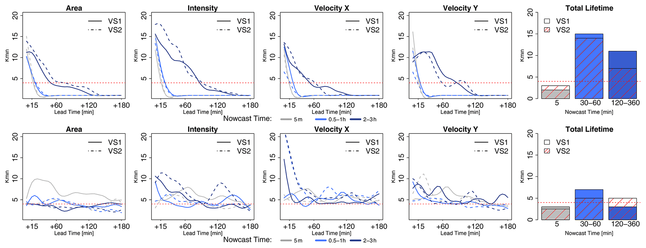
Figure 8 The optimization of the k-NN per target variable based on predictors and weights derived from Pearson correlation analysis: the median optimal selected “k” neighbours yielding the lowest absolute errors over the 110 events. Two k-NN applications are shown here – VS1 in solid line and VS2 in dashed line. First row – the optimal neighbour is found by minimizing the MAE for a given group of nowcast times per event. Second row – the optimal neighbour is found by minimizing the MAE for the given group of nowcast times per event. The red dashed horizontal line indicates the k=4 that is chosen in this study for the deterministic k-NN application.

Table 4 The median improvement of the total lifetime MAE when using k= 2–5 instead of k=1 over the three selected groups of nowcast times.

4.3 Results of the deterministic 4-NN nowcast

The median MAE of the 4-NN determinist nowcast over all the events, run for both target- and storm-based approaches, is shown in Fig. 9 for each lead time and target variable. The results are grouped according to the storm duration: (i) upper row – for storms that last for 30 min, (ii) middle row – for storms that last for up to 3 h, and (iii) lower row – for storms that last longer than 3 h and are averaged for nowcast times given in Table 2. As also shown in the optimization of the 4-NN, the target-based k-NN exhibits lower area, intensity, and velocity errors than the storm-based 4-NN. Table 5a illustrates the median deterioration (–) or improvement (+) in percent (%) over all lead times that the storm-based 4-NN can reach when compared to the target-based one.

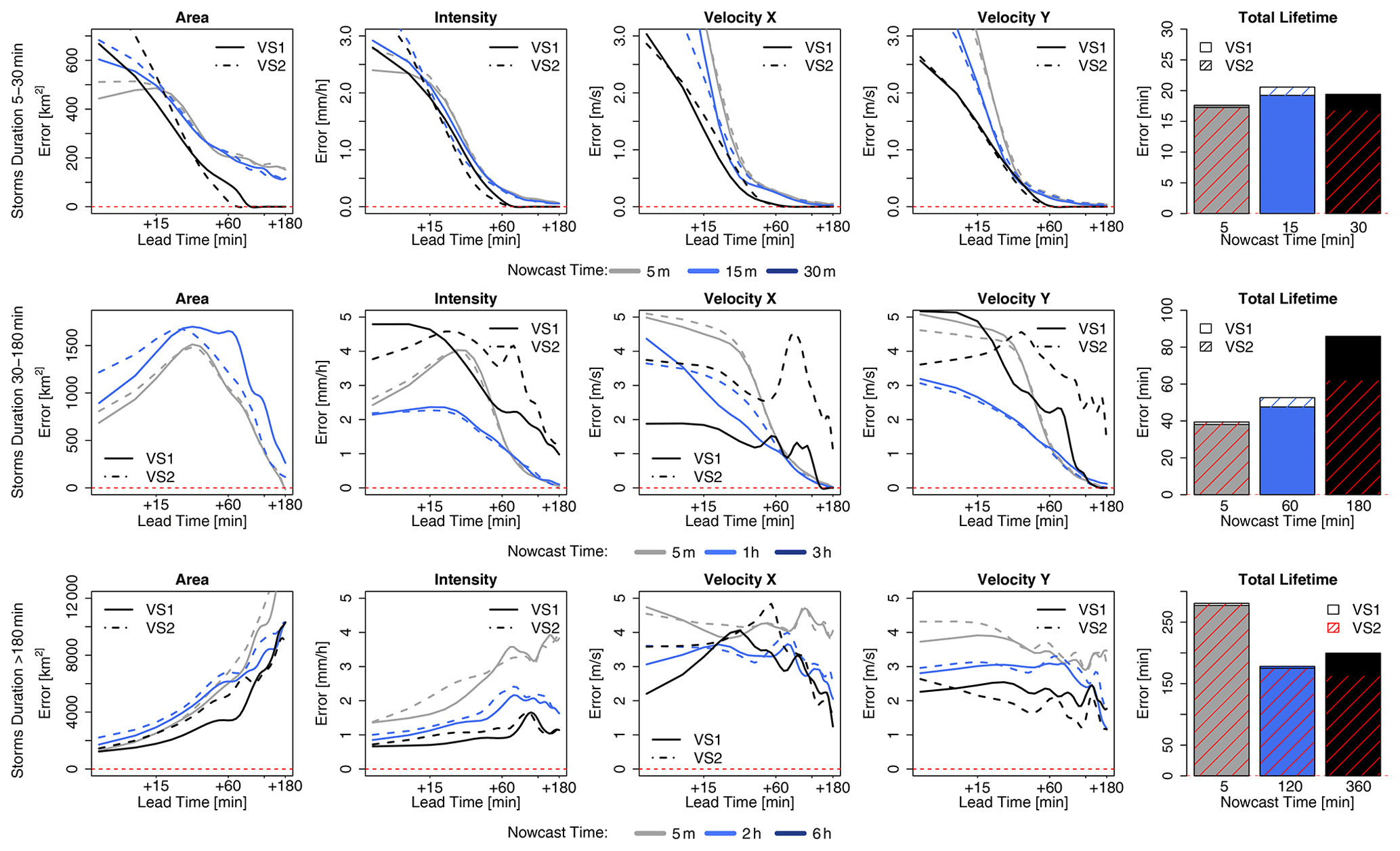
Figure 9 The median MAE over all the events for each target variable (area, intensity, and velocity in the x and y directions and total lifetime) based on two 4-NN applications: VS1 in solid and VS2 in dashed lines. The performance is shown for storms that are shorter than 30 min (upper row), shorter than 3 h (middle row), and longer than 3 h (lower row) and over the selected nowcast times. Nowcast time dictates when the nowcast is issued relative to storm initiation.

Table 5 Median deterioration (–) or improvement (+) of k-NN storm-based (VS2) compared to target-based (VS1) over all lead times according to the storm duration and nowcast times (shown in percentage). Equation (11) is used here, where “ref” is the target-based and “new” is the storm-based k-NN.

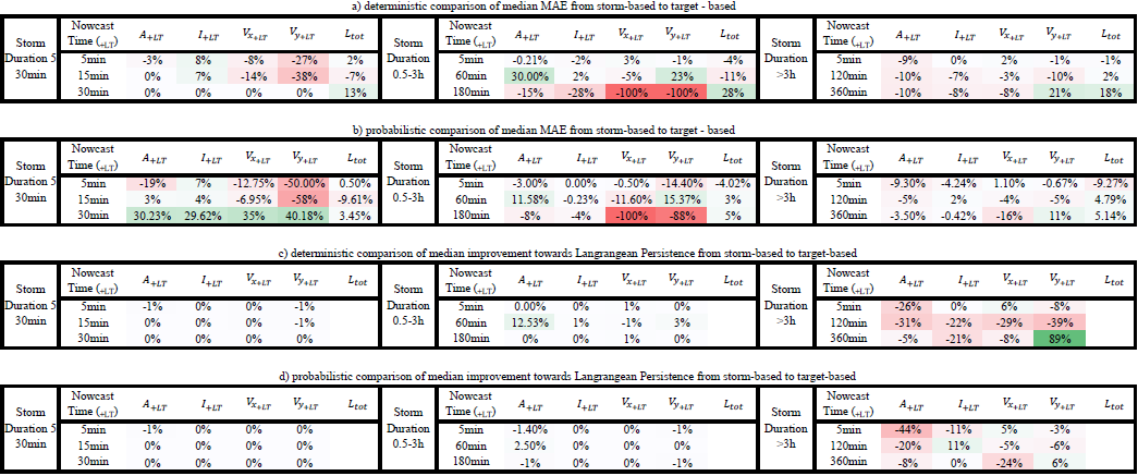
For storms lasting less than 30 min, the MAE decreases with the lead time, and past LT + 30 min is mostly zero, as the dissipations of the storms have been captured successfully. The total lifetime of the majority of the storms can be captured with ∼15 min overestimation/underestimation regardless of the nowcast time. The errors for the four target variables (except total lifetime) are lower for the later nowcast times than for the earlier ones (as expected). The difference between the storm- and target-based 4-NN is very small for area, intensity, and total lifetime but much higher for the velocity components (with the storm-based one exhibiting up to 40 % higher errors than the target-based one). The biggest difference seems to be for shorter lead times (LT <+1 h). For the storms lasting up to 3 h, the same behaviour is, more or less, observed. The only difference is for nowcasts issued at the third hour of the storm's existence (last moment the storm is observed). Here it is clear that the 4-NN fails to capture the dissipation of the storms that last exactly 3 h; however, this is attributed to the number of available storms with durations of 3 h (median over six storms available). Since the area, intensity, and total lifetime are overestimated and do not converge to zero for high lead times, it is clear that the nearest neighbours are being selected from the longer storms that do not dissipate within the next 3 h. The differences between the two 4-NN approaches are visible mainly for lead times of up to 30 min (except the nowcast at the third hour of a storm's life); afterwards, the errors relatively converge to each other. The storm-based 4-NN produces circa 10 %–20 % higher errors than the target-based one for the nowcast times lower than 3 h, while for the nowcast time of 3 h, the errors are up to 100 % higher than the target-based one. At these storms as well, the higher discrepancy between the two versions of 4-NN is seen at the velocity components.

For the storms that last longer than 3 h (of the 100 storms available), the same problem as in the nowcast time of 3 h seen before is present. The total lifetime is clearly underestimated (up to 100 min) as due to the database the information is taken from shorter storms. It is important to notice here, that, although 70 storms are present, because of the leave-one-event-out validation, the storm database is actually smaller. Nevertheless, the error is manifested here differently: as the long storms are more persistent in their features, area, intensity, and velocity components are captured better for the short lead times with the error increasing at higher lead times. Here too the nowcast issued at the earlier stages of the storm's life exhibits higher errors than in the later stages. Especially for the nowcast at the sixth hour of the storm's existence, the errors are quite low for all five target variables due to the persistence of the stratiform storms. For this group of long storms, the storm-based nowcast yields up to 10 % higher errors than the target-based one, with only a few exceptions depending on the time of nowcast and variable. It is clear that the storm-based 4-NN is more influenced by the number of available storms than the target-based approach.

Figure 10 shows the improvement that the 4-NN introduces to the nowcast when compared to the Lagrangian persistence (either target- or storm-based) and is averaged per lead time for each of the three groups of storms and the respective times of nowcast. Since the Lagrangian persistence does not issue a total lifetime nowcast, only the four target variables (area, intensity, and the velocity components) are considered. The green area indicates the percent of improvement from the application of the 4-NN approach, and the red area indicates the percent of deterioration from the 4-NN application (Lagrangian persistence is better). Additionally, median improvements (+) or deterioration (–) over all lead times of the storm-based approach compared to the target-based 4-NN approach with respect to the Lagrangian persistence are illustrated in Table 5c. For the 30 min storms, the 4-NN approaches (both target- and storm-based) are considerably better than the Lagrangian persistence: improvement is higher than 50 % from LT + 15 min and up to 100 % from LT + 60 min. The improvement is greater for nowcast at the 15th minute of storm existence (when the persistence predictors are considered). It is clear that, due to the autocorrelation, the Lagrangian persistence is more reliable for the short lead times and for earlier nowcast times. However, after LT + 15 min and for nowcast times near the dissipation of the storms, where the non-linear relationships govern, the improvements from the nearest neighbour are more significant. The target-based 4-NN results in slightly higher improvements than the storm-based one only for lead times up to 30 min: past this lead time the improvements from both versions converge. For the storms that last between 30 min and 3 h, the improvements are introduced first after LT + 15 or +30 min depending on the nowcast time: increasing nowcast time increases the improvement as well. The only exception is for the nowcast of area and intensity in the third hour of the storm's existence, where no clear improvement of the 4-NN approaches could be seen before LT + 30 min or LT + 1 h. This low improvement for the nowcast time of 3 h was expected following the poor performance of the 4-NN shown in Fig. 9. It seems like the Lagrangian persistence is particularly good for predicting the area and intensity at very short lead times (up to LT + 20 min). Here, for nowcast times of 5 min, the Lagrangian persistence is 100 % better than any of the 4-NN approaches, but the same is not true for the velocity components, with the Lagrangian persistence exhibiting very low advantages against the 4-NN for the short lead times. Regarding the difference of the two 4-NN approaches, with few exceptions, the storm-based nowcast exhibits similar improvements to the target-based one. Another exception is the nowcast time of 3 h, where the storm-based improvements are clearly lower, especially for the higher lead times, than the target-based ones (up to 40 %). For storms lasting longer than 3 h, the improvements are present for lead times higher than 2 h. Since the features of the long storms (mostly of a stratiform nature) are persistent in time, it is understandable for the Lagrangian persistence to deliver better nowcasts up to LT + 2 h. Past this lead time non-linear transformations should be considered. Here, even though the storm database is small, the non-linear predictions based on the 4-NN capture better these transformations than the persistence. The improvement introduced by the storm-based one are generally 20 % to 30 % lower than the improvements introduced by the target-based one.

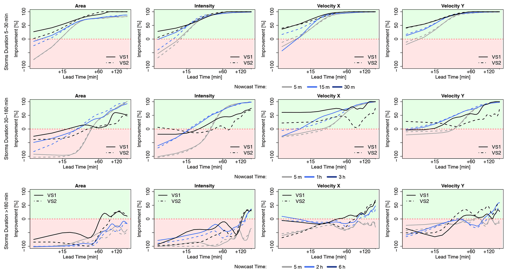
Figure 10 The median improvements over all the events that the single 4-NN application can introduce in the nowcast of the target variables (area, intensity, and velocity in the x and y directions) in comparison to the Lagrangian persistence. The results are shown for each 4-NN application: VS1 in solid and VS2 in dashed lines and calculated separately for storms that last for less than 30 min (upper row), less than 3 h (middle row), and more than 3 h (lower row) and for the respective nowcast times. The green region of the plot indicates a positive improvement (better nowcast by the 4-NN application), and the red region indicates a deterioration (better nowcast by the Lagrangian persistence).

To conclude, the 4-NN deterministic nowcast brings up to 100 % improvements for lead times higher than the predictability limit of the Lagrangian persistence and depends mainly on the storm type and the size of the database. Overall, for all storms the improvement is mainly at the high lead times and later times of nowcast, as the 4-NN captures particularly well the dissipation of the storms. The results from the long events suffer the most from the small size of the database. This was anticipated, as the events were mainly selected from convective events that have the potential to cause urban floods. A bigger database, with more stratiform events included, can introduce a higher improvement to the Lagrangian persistence. These improvements are expected to be higher for lead times longer than 2 h but are yet to be seen if a larger database can also behave better than the persistence even for lead times shorter than the predictability limit. Regarding the two different 4-NN approaches, the storm-based nowcast performs 0 %–40 % worse than the target-based nowcast, introducing generally 40 % lower improvements to the Lagrangian persistence. The main differences between these two approaches lie between the growth and decay processes, which the target-based 4-NN can capture better. Also, these differences are particularly larger for the velocity components and for the total lifetime than in the area and intensity as target variables. Furthermore, it seems that the storm-based 4-NN is more susceptible to the size of the database than the target-based one. Nevertheless, there are some cases where the storm-based nowcast behaves better than the target-based nowcast (as illustrated with green in Table 5a), even though the target-based approach should be profiting more from the selected predictors and their respective weights. A better-optimized K_min for each lead time and nowcast time may actually improve further on the results of both 4-NN versions and give the advantages mainly to the target-based nowcast.

4.4 Results of the ensemble 30-NN nowcast

The median CRPS over all the events for the probabilistic 30NNs (in solid lines) together with the median MAE for the deterministic 4-NN (in dashed lines) are illustrated respectively for the storm-based approach in Fig. 11 and for the target-based approach in Fig. 12. The results are shown as in the previous figures for each lead time and target variable for storms divided into three groups according to their duration and averaged depending on the time of nowcast. Additionally, the median improvements (+) or deterioration (–) of storm-based CRPS values in comparison to the target-based ones are given in Table 5b. For the 30 min-long storms, the errors of the probabilistic nowcast are typically lower than the single 4-NN nowcast for all the variables, lead times, and nowcast times, independent of the 30NNs approach (either storm- or target-based). In contrast to the deterministic 4-NN, the probabilistic 30NNs performance is not very dependent on the nowcast time (mainly for area, intensity, and total lifetime). The storm-based 30NNs have up to 50 % higher errors than the target-based ones but on the other hand can have up to 40 % lower errors than the target-based ones for nowcast times of 30 min. This suggests that storms of this duration behave similarly, and their dissipation can be predicted adequately by the storm-based approach with more than four similar neighbours. For storms that last less than 3 h, the same performance is also exhibited: the probabilistic 30NNs have lower errors than the deterministic 4-NN. The difference between the target- and storm-based nowcasts is within the range of the single 4-NN nowcast for the first four target variables, with storm-based 30NNs having 15 % higher errors in the first 30 min of the nowcast than the target-based ones. For intensity and the total lifetime, both of the 30NNs exhibit very similar errors for most of the nowcast times. It is worth mentioning here that for the nowcast at the third hour of storm existence the errors are much lower than the single 4-NN nowcast. This proves that the most similar storms are within the 30 members but not within the first four neighbours selected in the case of the single 4-NN nowcast. Due to the non-representativeness in the database, the errors of the longer storms are considerably higher than the other storm groups, and the errors of the first four target variables increase with the lead time and decrease with the nowcast time, as in the case of the deterministic 4-NN nowcasts. However, here, unlike the other storm groups, the differences between the storm-based and target-based approaches are visible past a 30 min lead time, with the storm-based errors being up to 15 % higher than the target-based ones.

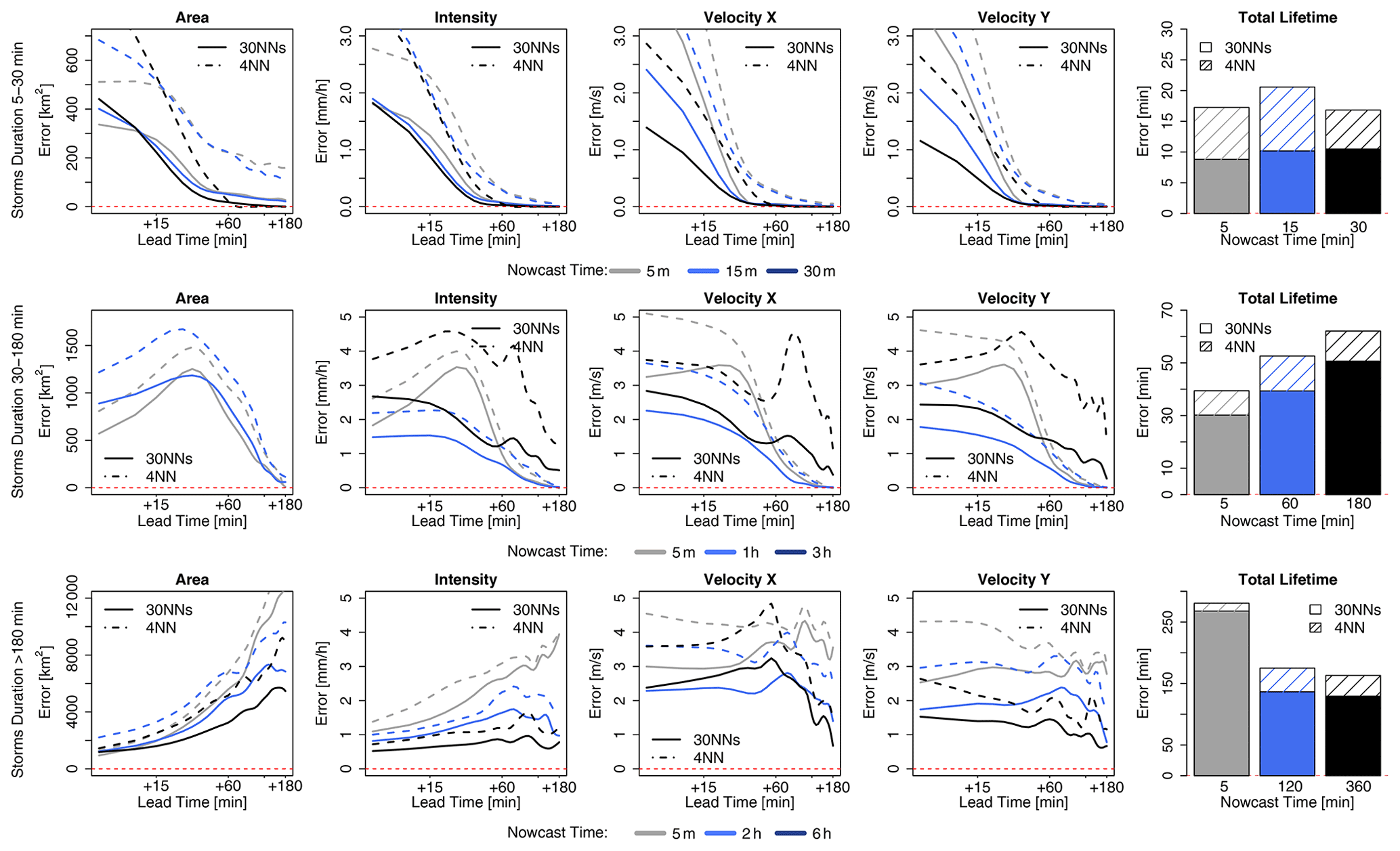
Figure 11 The median CRPS over all the events for each target variable (area, intensity, and velocity in the x and y directions and total lifetime) in the storm-based applications: 4-NN (deterministic) in dashed and 30NNs (probabilistic) in solid lines. The performance is computed over storms that are shorter than 30 min (upper row), shorter than 3 h (middle row), and longer than 3 h (lower row) and over the selected nowcast times.

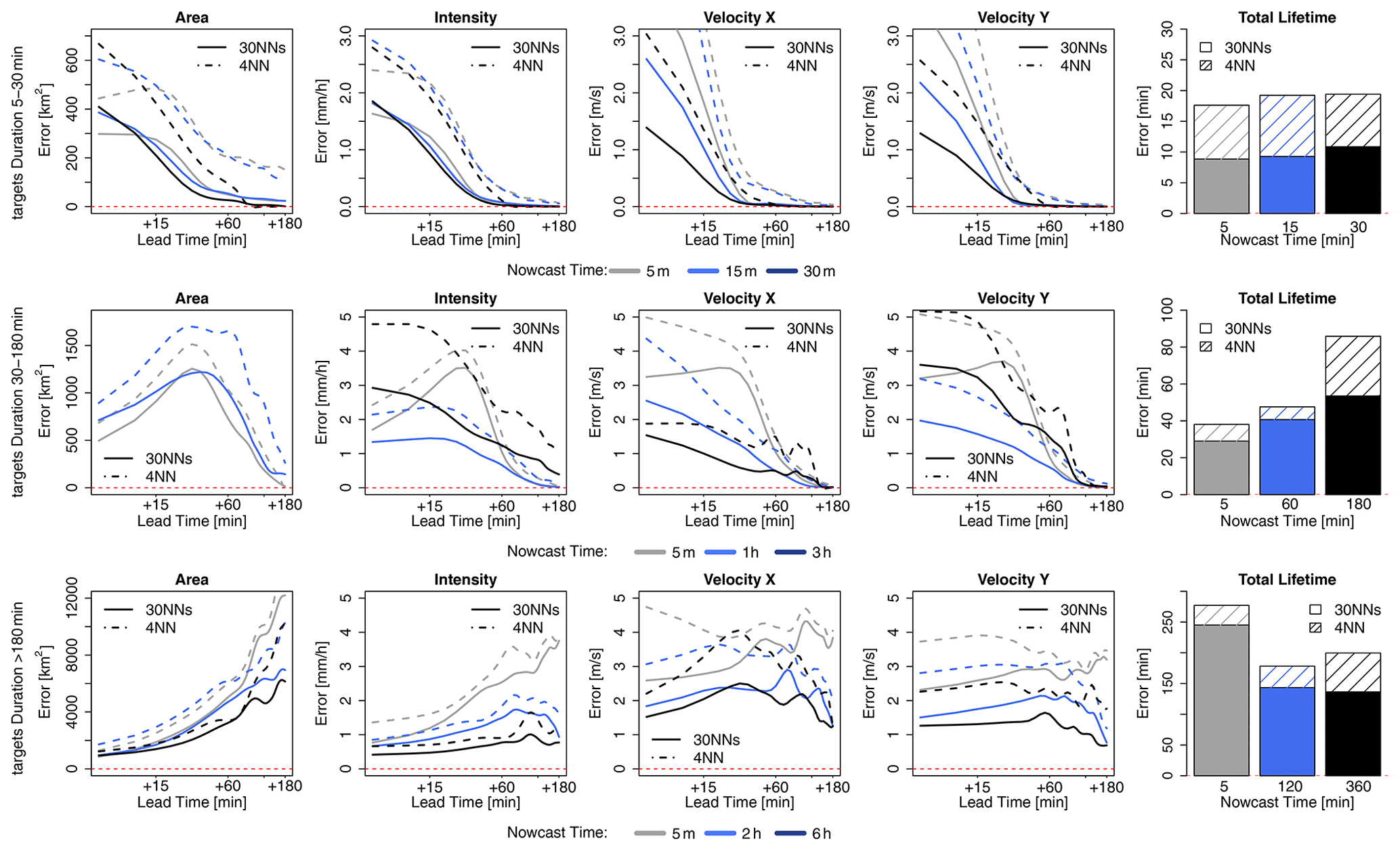
Figure 12 The median CRPS over all the events for each target variable (area, intensity, and velocity in the x and y directions and total lifetime) in the target-based applications: 4-NN (deterministic) in dashed and 30NNs (probabilistic) in solid lines. The median errors are computed over storms that are shorter than 30 min (upper row), shorter than 3 h (middle row), and longer than 3 h (lower row) and over the selected nowcast times.

Overall, the ensemble results are clearly better than the single 4-NN nowcast, suggesting that the best responses are obtained by singular neighbours (either the closest one or within the 30 neighbours) and not by averaging. Thus, there is still room for improving the single 4-NN nowcast by selecting better the important predictors and their weights or averaging differently the nearest neighbours. Nevertheless, the results from Figs. 11 and 12 emphasize that similar storms do behave similarly and that the developed k-NN in the given database with 30 ensembles gives satisfactory results. Compared to the deterministic 4-NN, it has the advantage that no k-optimization is needed, and the two approaches (storm- and target-based) have fewer discrepancies with one another.

Figure 13 demonstrates the improvement of the probabilistic 30NNs when compared to the Lagrangian persistence (storm-based in dashed line and target-based in solid line). As before, the median improvement over the events is computed and shown for each storm duration group, nowcast time, lead time, and target variable (expect for the total lifetime). For all three groups it is clear that performance increases considerably with the lead time, suggesting that the ensemble predictions are particularly useful for the longer lead times where the single nowcast is not able to capture the storm evolution. For short storms (duration shorter than 30 min), the Lagrangian persistence is only better for the area and intensity at 5 min nowcast time and for very short lead times (up to 10 min). However, past this lead time, the probabilistic 30NNs have the clear advantage, with improvements up to 100 %. Past LT + 30min, which coincides with the predictability limit of the Lagrangian persistence at such scales, there is no difference between the nowcast time and the 30NNs approach (less than 1 % for all target variables and nowcast times). For storms that last less than 3 h, the results are slightly worse than the very short storms but still exhibit the same patterns. Here too the main improvements of the 30NNs probabilistic approach is seen between LT + 15 min and LT + 30 min for all the target variables. In this storm group it is interesting that the results from the nowcast time of 3 h exhibit different behaviours than the deterministic approach. This is expected as the Lagrangian persistence performs particularly poorly because it cannot model the storm dissipations. The difference between the two types of 30-NN is insignificant although a bit higher than for the very short storms (∼2.5 % difference). For the longer storms the benefit of the probabilistic 30NNs is seen mainly for LT + 60 min to LT + 120 min but is still not as high as in the other storm groups. The worse performance is at a nowcast time of 5 min, where the 30NNs fail to bring any advantage to the prediction of area and intensity when compared to the Lagrangian persistence. It is interesting from these storms that the improvement is more significant at the velocity components than in the area and intensity predictions. This suggests that the velocity components are more persistent (see Fig. 4) and easier to predict from similar storms.

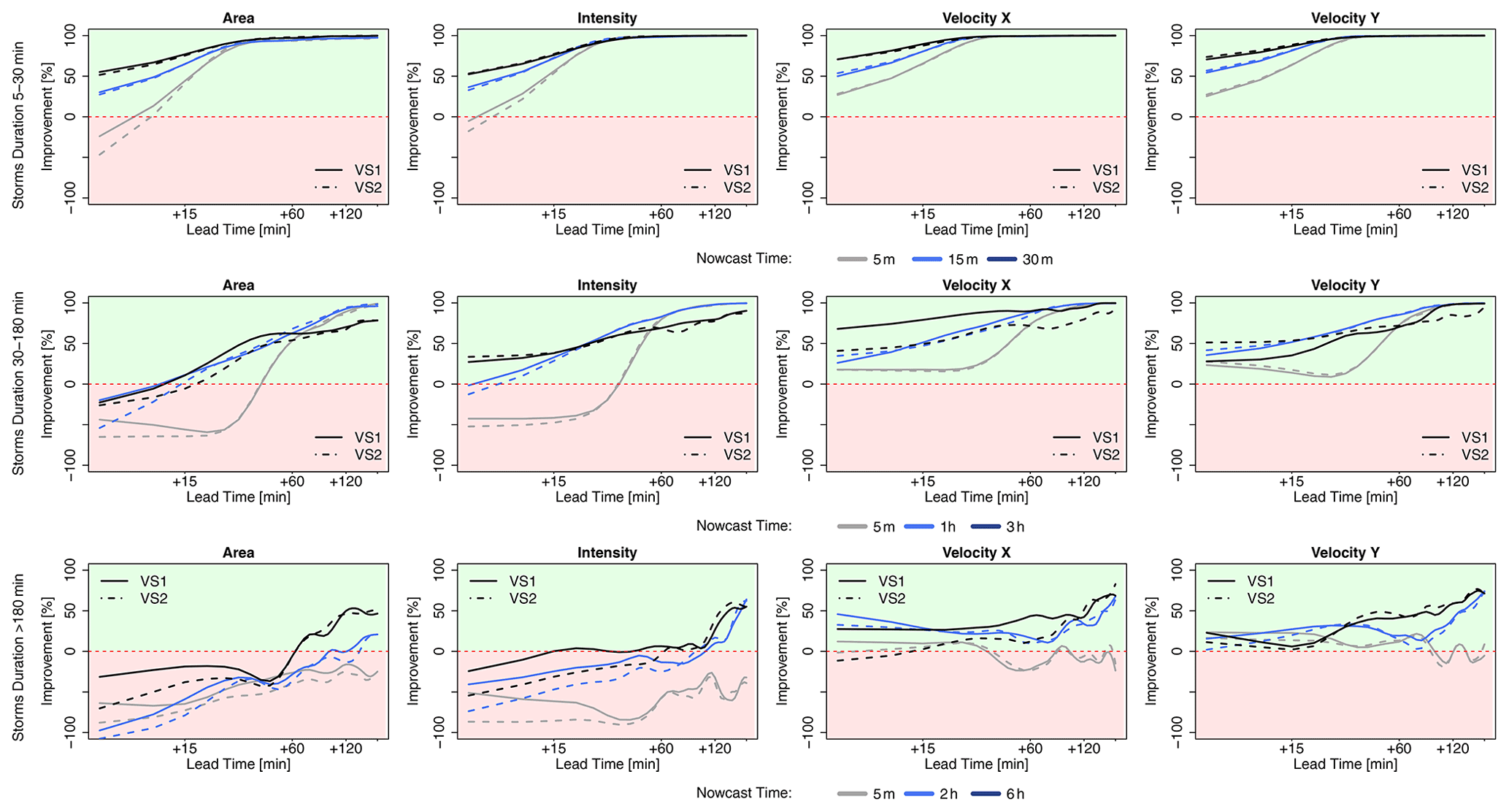
Figure 13 The median improvements over all events that the 30NNs nowcast can introduce into the nowcast of the target variables (area, intensity, and velocity in the x and y directions) in comparison to the Lagrangian persistence. The results are shown for each 30NNs application, VS1 in solid and VS2 in dashed lines, and are calculated separately for storms that last for less than 30 min (upper row), less than 3 h (middle row) and more than 3 h (lower row) and for the respective nowcast times. The green region of the plot indicates a positive improvement (better nowcast by the 4-NN application) and the red region indicates a deterioration (better nowcast by the Lagrangian persistence).

As a conclusion, the probabilistic nowcasts are better than the Lagrangian persistence mainly for convective storms that last less than 3 h and lead times longer than LT + 15 min. Of course, there is still room for improving the 30NNs application by increasing the size of the past database. Overall, it seems that the velocity components can be captured much better by the 30NNs application than the Lagrangian persistence, while the Lagrangian persistence is more suitable for long persistent storms and for nowcast times of 5 min, where not enough information is available to select similar storms. An increase in the database, with more stratiform storms, may improve the performance of the 30NNs and its advantage over the Lagrangian persistence. However, the value of the probabilistic 30NNs relies mainly on the nowcasting of convective events. Moreover, the possibility of merging Lagrangian persistence with a probabilistic 30NNs approach should be explored and further investigated; the Lagrangian persistence should be implemented for very short lead times (up to 30 min) and for the first nowcast times where the predictors are not enough to select similar past storms.

4.5 Nowcasting the unmatched storms

For the optimization and testing of the k-NN approaches, the unmatched storms from the tracking algorithm were left outside of the database. Nevertheless, in an online application (operational nowcast), when the storm is recognized for the first time, one cannot predict whether the storm will be an artefact or whether it will not be matched by the tracking algorithm. Therefore, it is important to investigate how the developed k-NN deals with these unmatched storms. Figure 14 illustrates the median performance over the 110 events of the developed target-based (upper row) and storm-based (lower row) k-NN when predicting the target variables of the unmatched storms from a past database of only matched storms (storms with duration equal to or longer than 10 min). As in the previous results, the 30NNs probabilistic application yields better errors than the deterministic one, causing an overestimation of these storms for the first 10–20 min for the target-based approach and 15–30 min for the storm-based one. A direct comparison of these errors with the Lagrangian persistence is shown in Fig. 15, with the deterministic 4-NN in the upper row and the probabilistic 30NNs in the lower row. As expected, the probabilistic 30NNs bring the most improvement when compared to the Lagrangian persistence for all lead times and target variables. Thus, even though most of these unmatched storms will be overestimated in their duration, the 30NNs will capture their dissipation much better than either the deterministic 4-NN or the Lagrangian persistence.

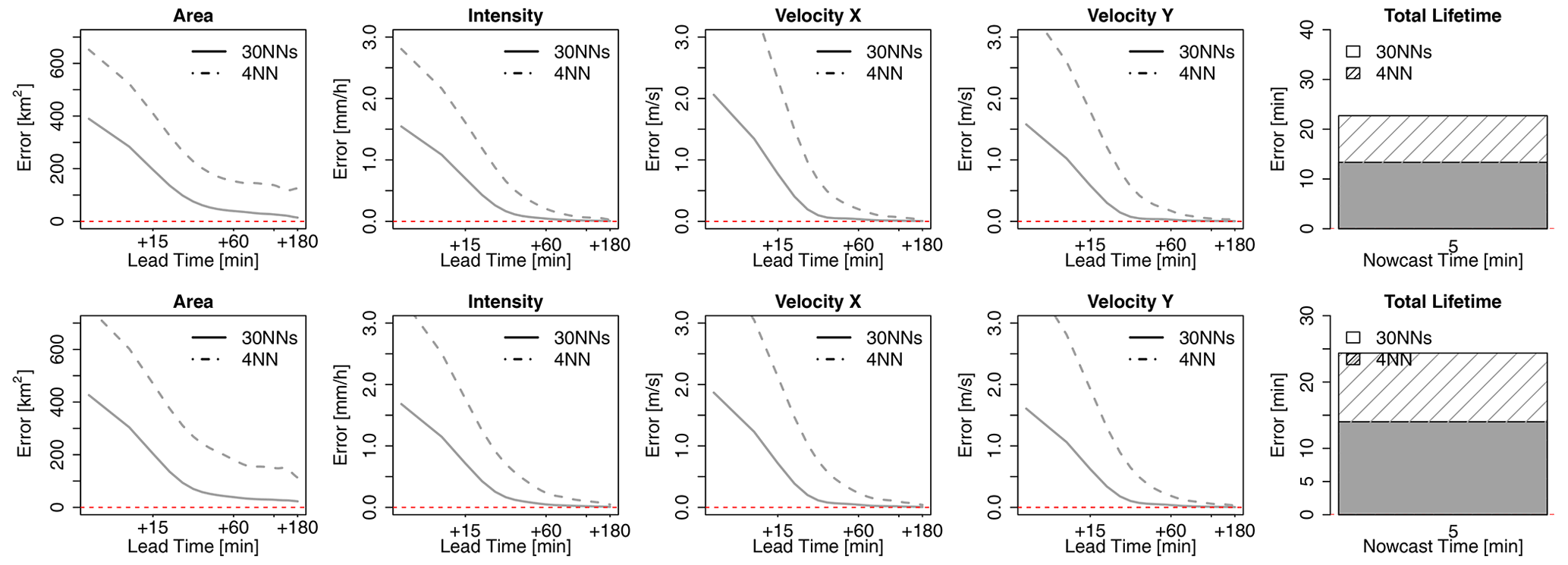
Figure 14 Median CRPS error over the 110 events for each of the target variables nowcasted from 4-NN deterministic (in dashed lines) and 30NNs probabilistic (in solid lines) applications for both target- (upper row) and storm-based (lower row) approaches. The results shown here are from the “unmatched storms” when the nowcast time is 5 min.

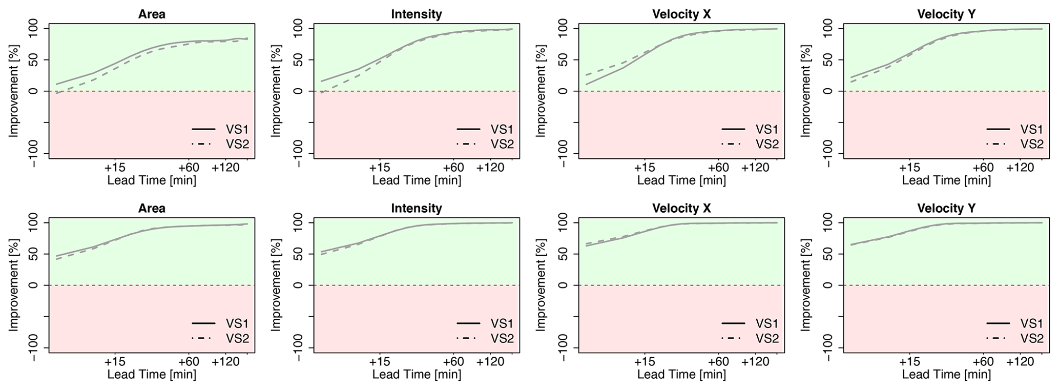
Figure 15 Median performance improvement over the 110 events for each of the target variables nowcasted from 4-NN deterministic (upper row) and 30NNs probabilistic (lower row) applications when compared to the Lagrangian persistence for both target- (dashed line) and storm-based (solid line) approaches. The results shown here are from the “unmatched storms” when nowcast time is 5 min.

5 Conclusions

Accurate predictions of rainfall storms at fine temporal and spatial scales (5 min, 1 km²) based on radar data are quite challenging to achieve. The errors associated with the radar measurements, identification, and tracking of the storms and more importantly the extrapolation of the storms in the future based on the Lagrangian persistence limit the forecast horizons of such object-oriented radar-based nowcasts to 30–45 min for convective storms and to 1 h for stratiform events (Shehu and Haberlandt, 2021). The focus of this paper was the improvement of the storm-oriented radar-based nowcasts by considering other non-linear behaviours for future extrapolation instead of Lagrangian persistence. For this purpose, a nearest-neighbour approach was proposed that predicts future behaviours based on past observed behaviours of similar storms. The method was developed and validated for the Hanover Radar Range, where storms from 110 events were pooled together and used in a “leave-one-event-out” cross-validation. From 110 events a total of around 5200 storms with different morphologies were identified and tracked with HyRaTrac in order to build up the database for the k-NN implementation. The storms were treated as ellipses, and for each state of the storms' evolution different features (describing both present and past states) were computed. The k-NN approach was developed on these features to predict the behaviour of the storms in the future (for lead times up to 3 h) through five target variables (area, intensity, velocities in the x and y directions, and total lifetime).

First an importance analysis was performed in order to recognize the most important predictors for each target variable. Two different approaches were employed for this purpose: Pearson correlation and partial information correlation (PIC). A comparison of these two methods revealed that for the application at hand Pearson correlation is more reliable at determining important predictors and delivers 5 %–30 % better results than the PIC method. However, the PIC seems promising mainly for determining the most important predictors of the area and total lifetime for storms longer than 3 h and is still recommended for investigation in the future. The area, intensity, and total lifetime of the storms seem to be co-dependent on one another and on the features that describe their evolution. In particular, the variance of the spatial intensity is an important predictor for the three of them. On the other hand, the velocity components are dependent more on features that describe their evolution. Nevertheless, there is still a dependency of the area and velocity components, and this should be included when predicting each other, mainly for long lead times.

The weights derived from the Pearson correlation were used for the similarity estimation of different storms based on the Euclidian distance. Two k-NN approaches were developed on two similarity metrics: (a) target-based approach – similarity was computed for each target independently and indicates the best performance possible by the given predictors and weights; (b) storm-based approach – similarity was computed for each storm, keeping the relationship between the target variables. For the two approaches a deterministic (averaging the 4 nearest neighbours) nowcast and a probabilistic (with the 30 nearest neighbours) nowcast were issued for all of the storms in leave-one-event-out cross-validation mode. In the deterministic nowcast the difference between the two remains mainly at short lead times (up to 30 min) and at the velocity components, with the storm-based results yielding up to 40 % higher errors than the target-based ones. However, at higher lead times the difference between the two became insignificant, as the dissipation processes were captured well for the majority of the storms. The same behaviours were observed as well in the ensemble nowcast, with target-based ensembles being slightly better than the storm-based nowcast. Overall, the storm-based approach seems reasonable for area, intensity, and total lifetime, as they are co-dependent and their relationship should be maintained for each storm, while the target-based approach captures better the velocity components. A combination of both approaches may result in better nowcasting of storm characteristics.

To investigate which value each of the two k-NN approaches introduces to the nowcast, their errors (for both deterministic and probabilistic nowcast) were compared to the errors produced by the Lagrangian persistence. For both of the approaches the improvement was more than 50 % for convective storms for lead times higher than 15 min and for mesoscale storms for lead times higher than 2 h. The results were particularly good for the small convective storms due to the high number of storms available in the database. For the mesoscale storms (with duration longer than 3 h), the improvements were not satisfactory due to the small sample size of such long storms. Increasing the sample size is expected to improve the performance of the k-NN for these storms as well. However, when consulting the probabilistic k-NN application it seems that, even for these storms and the given database, there are enough similar members in the 30 neighbours that are better than the Lagrangian persistence. This emphasizes that the probabilistic nowcast is less affected by the sample size than the deterministic 4-NN. Moreover, the differences between the storm-based and target-based approaches become smaller in the probabilistic approach than in the deterministic one. Lastly, the optimization of the adequate neighbours for the deterministic approach is far more complex than implemented here, but when issuing the probabilistic nowcast there is no need to optimize the k number. It is clear that the probabilistic application of the k-NN outperforms the deterministic one and has more potential for future works.

Overall, the results suggest that if the database is big enough, storms that behave similarly can be recognized by their features, and their responses are useful in improving the nowcast up to 3 h lead times. We recommend the use of the nearest neighbour in a probabilistic application (30NNs) to capture better the storm characteristics at different lead times. A merging with the Lagrangian persistence for short lead times (up to 15 min) and early nowcast times can also be implemented. Further improvements can be achieved if the predictor importance is estimated better (i.e. Monte Carlo approach or neural networks) or if additional predictors are included from other data sources like cloud information from satellite data, temperature, convective available potential energy (CAPE), and convective inhibition (CIN) from numerical weather prediction models, lightning flash activity, additional measurements from Doppler or dual-polarized radar data (like phase shift, Doppler velocity, vertical profile at different elevation angles), or various geographical information (such as distance from heavy urbanized areas, mountains, or water bodies). The main benefit of the probabilistic 30NNs is mainly seen for convective events and the creation of new nowcasting rules based on the predicted storm characteristics.

Improving the nowcasting of storm characteristics is the first step in improving rainfall nowcasting at fine temporal and spatial scales. In a second step, knowledge about the storm characteristics (as nowcasted by the 30NNs) should be implemented in the spatial structure of the storms to estimate rainfall intensities at fine scales (1 km² and 5 min). There are two options to deal with the spatial distribution of the rainfall intensities inside the storm region (which has so far not been treated in this study). (1) Increase/reduce the area by the given nowcasted area (as a target variable) for each lead time, scale the average intensity with the nowcasted intensity, and move the position of the storm in the future with the nowcasted velocity in the x and y directions. (2) Take the spatial information of the selected neighbours, perform an optimization in space (such that the present storm's and neighbour storm's locations match), and assign this spatial information to the present storm for each lead time. The former is an extension of the target-based 30NNs, while the later is an extension of the storm-based 30NNs. So far, the comparison between these two versions showed that the target-based approach is better suited mainly to nowcasting the velocity components, and thus a merging of the two could also be reasonable: the storm-based approach is used for nowcasting area–intensity–total lifetime (features that are co-dependent based on the life cycle characteristics of convective storms) and the target-based approach for the nowcasting of the velocity components. Future work (Part II – Point-scale rainfall intensities) will include the integration of the developed 30NNs application in the object-oriented radar-based nowcast to extend the rainfall predictability limit at fine spatial and temporal scales (1 km² and 5 min). The main focus of Part II will be to investigate whether the methodology applied here can also introduce improvements at the local scale, i.e. validation with the measurements from the rain-gauge observations.

Appendix A

Table A1 Strength of the relationship between the selected predictors and the target variables averaged for three lead times and storm duration groups based on correlation values. The green shade indicates the strength of the relationship, with 0 for no relationship at all and 1 for the highest dependency. The averaged computed values for each target variable (last row) are used as bases for Table 3. The correlation weights are absolute values of the correlation values between the predictors at specific lead times and target variables.

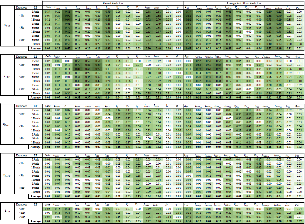
Table A2 Strength of the relationship between the selected predictors and the target variables averaged for three lead times and storm duration groups based on the PIC method. The green shade indicates the strength of the relationship, with 0 for no relationship at all and 1 for the highest dependency. The averaged computed values for each target variable (last row) are used as bases for Table 3: for intensity and velocity in the x and y directions, since the PIC recognized only one predictor as important, and the average value is given as 1 for the selected respective predictor.

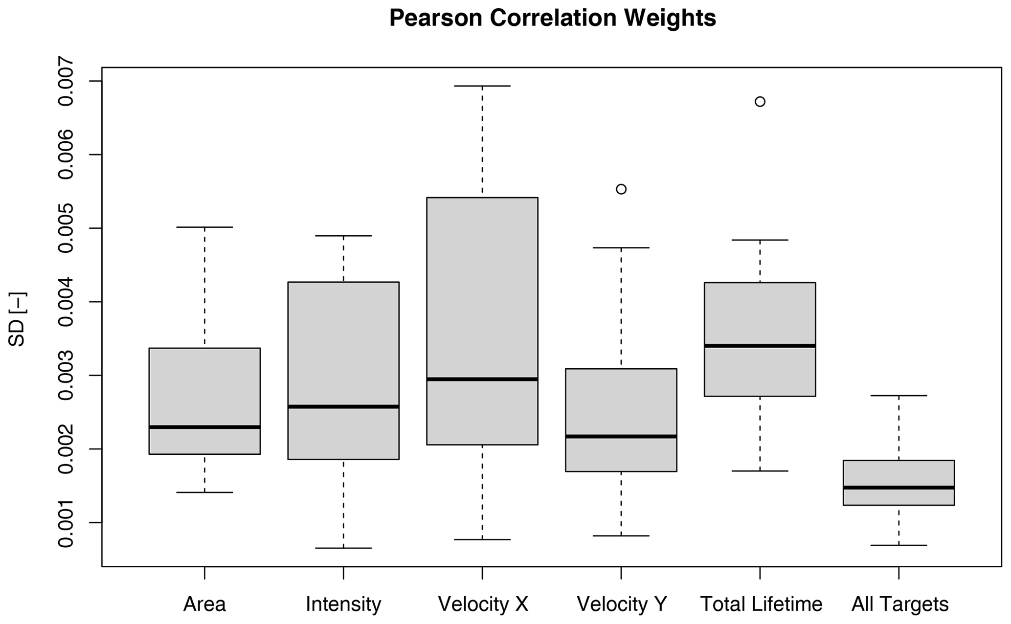
Figure A1 The standard deviation of the Pearson correlation weights between predictors and target variables obtained from a cross-sampling of the events (leave one event at a time out). The box plot for each target variable describes the spread of the standard deviation over all selected predictors.