the Creative Commons Attribution 4.0 License.
the Creative Commons Attribution 4.0 License.
 | 03 Feb 2021
Quantifying the impacts of compound extremes on agriculture
Danielle S. Grogan
Thomas W. Hertel
Wolfram Schlenker
Agricultural production and food prices are affected by hydroclimatic extremes. There has been a growing amount of literature measuring the impacts of individual extreme events (heat stress or water stress) on agricultural and human systems. Yet, we lack a comprehensive understanding of the significance and the magnitude of the impacts of compound extremes. This study combines a fine-scale weather product with outputs of a hydrological model to construct functional metrics of individual and compound hydroclimatic extremes for agriculture. Then, a yield response function is estimated with individual and compound metrics, focusing on corn in the United States during the 1981–2015 period. Supported by statistical evidence, the findings suggest that metrics of compound hydroclimatic extremes are better predictors of corn yield variations than metrics of individual extremes. The results also confirm that wet heat is more damaging than dry heat for corn. This study shows the average yield damage from heat stress has been up to four times more severe when combined with water stress.
- Article
(2295 KB) - Full-text XML
-
Supplement
(1206 KB) - BibTeX
- EndNote


The United States is the world's top food exporter, being the major producer of global calories of the four staple crops of corn, soybeans, wheat, and rice, which together account for 75 % of the calories humans consume (USDA–NASS, 2017). Specifically, it produces more than 40 % of the world's corn. Precipitation and temperature weather extremes cause variations in crop yields, affecting not only crop growth but also crop prices and farm revenues. As climate changes, all regions of the planet are experiencing more frequent weather extremes – often with greater magnitude than in the past (WMO, 2013); the World Meteorological Organization (WMO) calls 2001–2010 the “decade of climate extremes”, and this time frame did not even include the record-breaking year 2012 that devastated corn and soybean production across the US (Rippey, 2015). This year was both very hot and very dry in many parts of the Corn Belt. To understand past and future global food security, it is therefore essential to quantify and build predictive models of the impacts of extreme weather events on staple crop yields.
The focus of this paper is statistical modeling of crop yields, (e.g., Schlenker and Roberts, 2009), which draws heavily on the field of econometrics. While there is also a rich literature of process-based crop yield models (Jones et al., 2017), many of these models still rely on observational data-derived statistical relationships between extreme weather events and yields to capture impacts of extremes. Additionally, recent high-visibility studies on the impact of weather extremes on past and future crop yields rely entirely on statistical econometric modeling (Lobell et al., 2013). The relationship between extreme heat and crop yields has been well documented, particularly across the United States (US) and for corn, the US's largest crop by acreage (Schlenker and Roberts, 2009; Urban et al., 2012; Diffenbaugh et al., 2012; Roberts et al., 2013; Lobell et al., 2013; Urban et al., 2015; Wing et al., 2015; Burke and Emerick, 2016). Statistical and process-based crop models also appear to agree on corn yield impacts due to heat (Liu et al., 2016; Tebaldi and Lobell, 2018).
However, there is less agreement and greater uncertainty around the crop yield impacts of hydrologic extremes, due largely to the use of annual or season mean precipitation metrics in statistical models that fail to capture hydrologic extremes (D'Odorico and Porporato, 2004; Lobell and Burke, 2010; Schaffer et al., 2015; Werner and Cannon, 2016). These cumulative indices – monthly mean or seasonal average precipitation – do not capture extreme events that occur within the season. For example, precipitation amounts from early season floods and late season droughts can cancel out when taking the average, effectively smoothing over these extreme events in the data. The computed mean for this variable can be misleading as crop growth responds to day-to-day variability. While average conditions are important, exposure to extreme water stress can cause permanent, unrecoverable damage to plants (Denmead and Shaw, 1960), while too much water can cause yield-damaging floods, waterlogging, or may wash out soil nutrients and fertilizers (Kaur et al., 2018; Schmidt et al., 2011; Urban et al., 2015).
Crops obtain most of their water directly from soil moisture, yet extreme water metrics based on soil moisture have been only minimally explored (Fishman, 2016). Several studies have highlighted the need for irrigation to compensate for soil moisture deficits (Li et al., 2017; McDonald and Girvetz, 2013; Meng et al., 2016; Williams et al., 2016), further pointing to soil moisture as a potentially more important crop water availability metric than precipitation. However, current statistical studies have had limited success in statistically capturing the yield response to soil moisture metrics (Bradford et al., 2017; Peichl et al., 2018; Siebert et al., 2017). There are several potential reasons for this limited success. First, direct measures of soil water availability include complex biophysical and hydrological processes that are difficult to capture in a rather simple statistical model. Another barrier has been the limited availability of daily fine-scale soil moisture data and the inconsistency of soil moisture data with heat information. It has, therefore, become a standard practice in statistical crop modeling either to focus on a limited geographical area (Rizzo et al., 2018; Wang et al., 2017) or to employ a proxy variable like precipitation, evapotranspiration, or vapor pressure deficit estimates (Comas et al., 2019; Roberts et al., 2013).
A few recent studies have highlighted the importance of mean soil moisture metrics for estimating crop yields in the US (Ortiz-Bobea et al., 2019; Ribeiro et al., 2020). However, Ortiz-Bobea et al. (2019) estimated the average impact of heat stress on corn yields without distinguishing between a hot dry day (dry heat) and a hot wet day (wet heat), and similarly, Ribeiro et al. (2020) evaluated the impacts of dry heat and ignored the impacts of wet heat stress. These papers do not focus on the interaction or compound effects. Therefore, there is currently no robust predictive framework that captures the implications of compound extremes which appear in the historical climate record and are expected to become more frequent under future climate change conditions (Myhre et al., 2019). It is important to build such a framework because harmful extreme heat can be less harmful when there is sufficient soil moisture (Hauser et al., 2019), indicating that previous estimates of extreme heat impacts on staple crop yields may be biased high.
This paper presents the first statistical predictive crop yield model that directly addresses the gap in our knowledge of crop yield impacts due to compound weather extremes, including both dry heat and wet heat. This is accomplished by using high-resolution, daily simulated soil moisture data that are consistent with daily temperature data and applied to corn yield data across the continental United States.
This paper introduces two statistical models of crop yield as a function of heat and soil moisture, effectively building on the regression model methods from Schlenker and Roberts (2009) and Ortiz-Bobea et al. (2019). While both of these studies considered similar metrics for heat, the former is based on precipitation, and the latter considers an average soil moisture metric. The current study extends them by introducing easy-to-use metrics of individual and compound extremes based on simulated soil moisture. Here, Model (1) assumes that the impacts of heat and water on corn yields are separable. This model considers metrics of individual extremes (heat stress and water availability). Relaxing the separability assumption, Model (2) assumes the yield impacts of heat and water are mutually interdependent. Model (2) considers metrics of compound extremes. Model (1) helps to estimate the marginal impact of heat stress (individual extreme) and the marginal impact of daily soil moisture stress (individual extreme) on crop yields. Model (2) provides a framework for measuring the conditional marginal impact of heat and soil moisture (compound extremes) on crop yields.
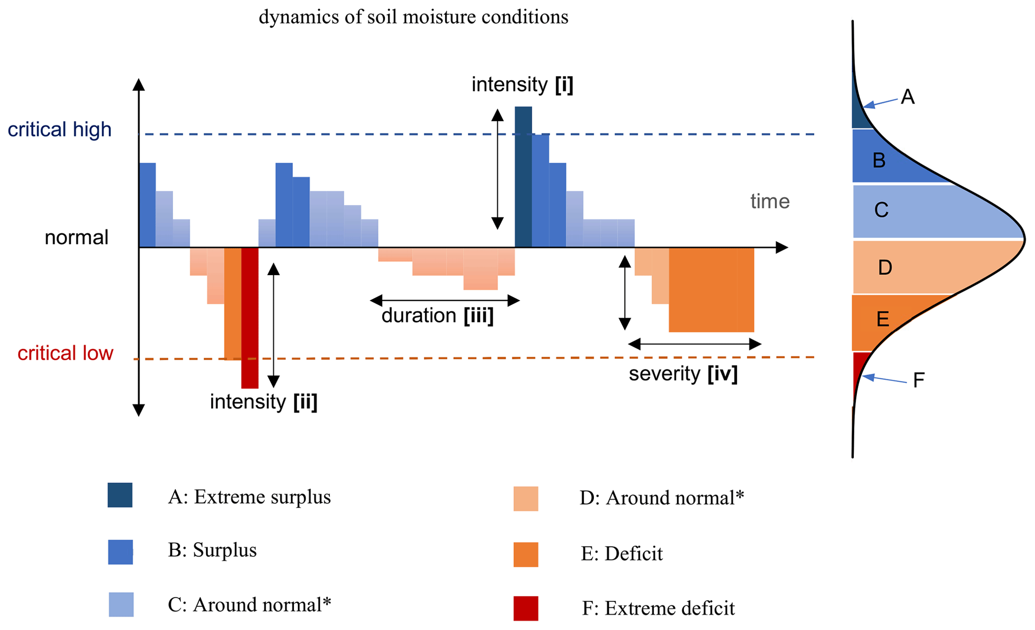
Figure 1Soil moisture dynamics within a typical growing season. Some soil moisture conditions can be harmful to crops, including excess wetness (i), moisture stress intensity (ii), duration of moisture stress (iii), and severity of soil moisture stress (iv). The around normal (*) levels can be determined by statistically examining the impacts of various intervals of soil moisture deviation from normal (seasonal mean volumetric soil moisture).
2.1 Data
In estimating the marginal impact of soil moisture on corn yields, we employ information about soil moisture, temperature, precipitation, and corn yields for counties of the United States for the 1981–2015 period. The data on yield are obtained from United States Department of Agriculture, National Agricultural Statistics Service (USDA–NASS) at the county level. The yield is defined as the corn production (in bushels) divided by harvested area (in acres). Precipitation is defined in millimeters as accumulated rainfall during the growing season (April–September). It is calculated based on PRISM (Parameter-elevation Regressions on Independent Slopes Model) daily information at 2.5×2.5 arcmin grid cells over the continental US for 1981–2015. It is aggregated to each county according to cropland area weights. Compound metrics of heat and soil moisture are also calculated daily at the gridded level. Then, we aggregate the metrics to the growing season and county level. Daily soil moisture content and soil moisture fraction are obtained from the Water Balance Model (WBM; Grogan, 2016; Wisser et al., 2010), based on daily simulations using PRISM data at 6×6 arcmin grid cells for the 1981–2015 period over the continental US.
2.2 Data processing
Major metrics used in this study are listed in Table 1. To derive the metrics listed in this table, the climate and soil moisture data are processed. The heat metrics are based on the concept of growing degree days (dday). Following D'Agostino and Schlenker (2015), the daily distribution of temperatures is approximated assuming a cosine function between the daily minimum and maximum temperature. Let , then dday at each day is defined using the following:
where b is the base for calculating dday and can take the base values and critical values. This study considers a piecewise linear function to aggregate the dday. The major assumption is that plant growth is approximately linear between two bounds. The dday between two bounds are simply dday above the smaller bound minus dday above the larger bound. The dday are initially calculated for each day at each 2.5×2.5 arcmin grid cell during the growing season (April–September). Then, they are aggregated for the whole growing season from the first day of April through the last day of September. Finally, they are aggregated to the county level using cropland area weights. We employ the Cropland Data Layer (CDL) from the US Department of Agriculture to exclude grid cells with no cropland and to aggregate the grid cell information to the county level (Boryan et al., 2012; USDA–NASS, 2017).
Table 1Major variables in each model of the study.
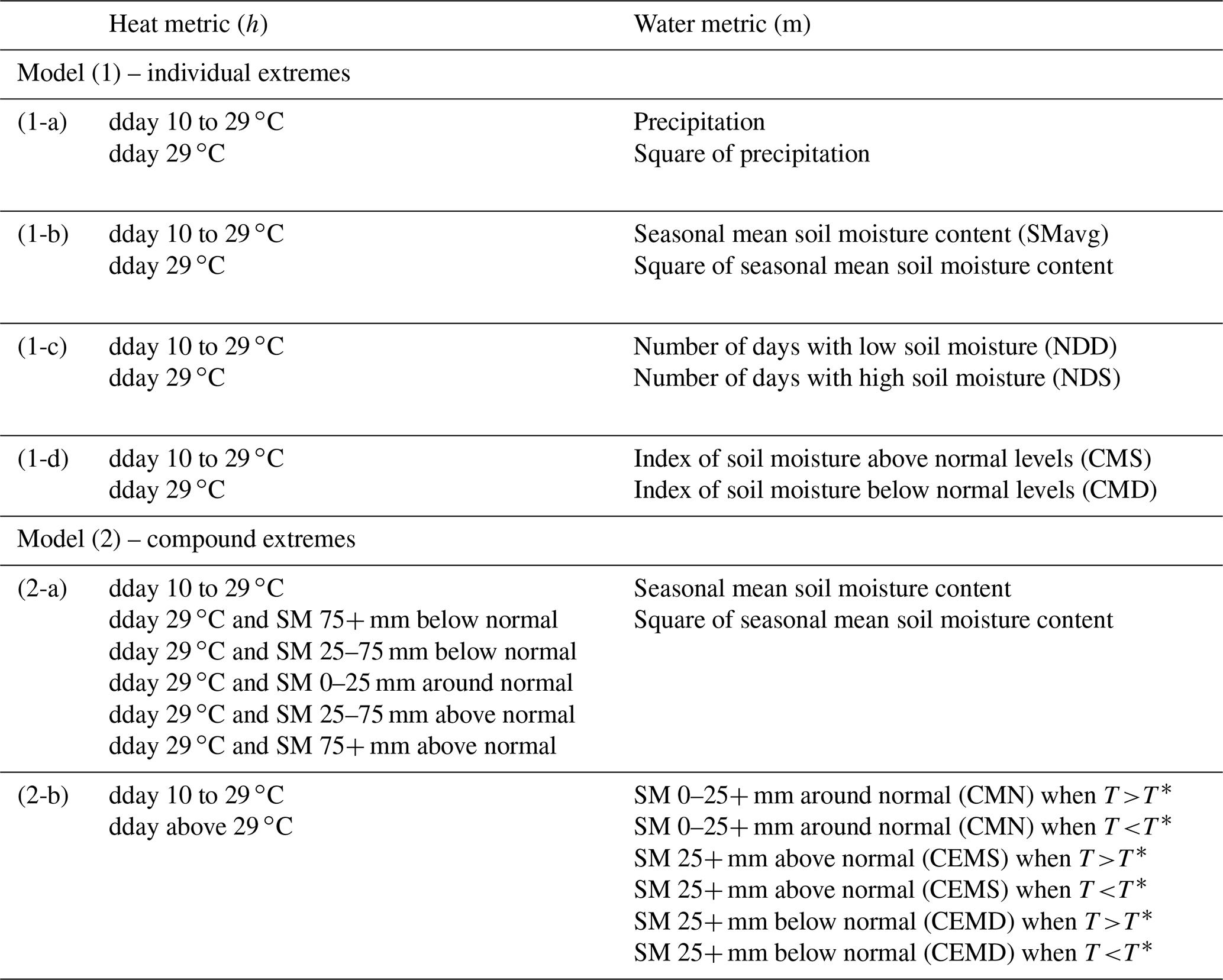
Note: dday – degree days; SM – soil moisture; SMavg – seasonal mean soil moisture; NDD – number of days when the soil moisture content is more than 25 mm below normal levels; NDS – number of days when the soil moisture content is more than 25 mm above normal levels; CMS – index of moisture surplus; CMD – index of moisture deficit; CMN – index of normal soil moisture; CEMS – index of extreme moisture surplus; CEMD – index of extreme moisture deficit. T* represents the temperature threshold.
The soil moisture metrics are constructed as the deviation from normal. Normal levels are defined as seasonal mean volumetric soil moisture over the 1981–2015 period. The water available to plants depends on volumetric soil moisture and soil type. To operationalize the soil moisture metric, this study considers the soil moisture deviation from normal. Soil moisture deviation is defined as daily soil moisture minus the normal soil moisture levels. Figure S1 in the Supplement shows the difference between normal soil moisture content, water available to plants, and unavailable water. The soil moisture level is considered extreme if it is below/above a threshold. The threshold is obtained by testing the impacts of 5 mm intervals of soil moisture deviation from normal.
Figure 1 visualizes soil moisture conditions as the basis for the construction of the soil moisture metrics (the legend in the figure is as follows: extreme surplus – A; surplus – B; around normal – C and D; deficit – E; extreme deficit – F). Three types of metrics are constructed for each condition. The simplest metric is the number of days during the growing season with each condition. To show the intensity of each condition, the second metric is defined based on the cumulative deviation from normal for each condition. Finally, a compound metric is defined as the sum of dday for each observed soil moisture condition. In Table 1, SMavg is calculated as the seasonal mean of soil moisture content (in millimeters for the 1000 mm topsoil) from the first day of April through the last day of September for each grid cell for each year. This metric shows the average soil moisture conditions. Then, NDD and NDS represent the number of days on which the daily volumetric soil moisture content is more than 25 mm below normal levels or is more than 25 mm above normal levels, respectively. Furthermore, CMS and CMD show the cumulative soil moisture surplus (above normal) and deficit (below normal) while CEMS and CEMD show the cumulative extreme soil moisture surplus (25+ mm above normal) and deficit (25+ mm below normal), respectively. These are metrics of extreme soil moisture conditions. Finally, CMN represents a cumulative metric of soil moisture index around normal.
2.3 Model (1) – individual extremes
Model (1) is a basic model that uses individual extremes, following a similar approach to Schlenker and Roberts (2009). Model (1) assumes that the effects of heat on corn yields are cumulative over the growing season and separable from water. In other words, the end-of-season yield is the integral of daily heat impacts over the growing season. This relationship can be demonstrated via Eq. (2) as follows:
where yit is the crop yield, g(h) is a function showing yield as a function of heat,φit(h) is the time distribution of heat (h) over the growing season in location i and year t, while the heat ranges between the lower bound and the upper bound . Metrics of water availability (e.g., precipitation or soil moisture) and other control factors are denoted as zit, and ci is a time-invariant fixed effect. All other unobserved variables are in the ϵit term. The fixed effect variable (also termed the unobserved individual effect) allows us to control for other biophysical or economic characteristics of each location which are not varying over time and can potentially explain the yield differences between counties. Note that this form of equation with fixed effects and unobserved variables is a standard econometric method. We evaluate the accuracy of this model, compared to historical data, first using cumulative precipitation and then mean soil moisture as the water availability metric zit.
For Model (1), different representations of water variables are considered. In Model (1-a), zit includes cumulative precipitation from the first day of April to the last day of September and its square term; this will evaluate the standard way in which yields have been estimated in previous studies. In Model (1-b), zit is the seasonal mean soil moisture index and its square term, which is used to evaluate the use of soil moisture instead of precipitation. Model (1-c) includes the number of days with low soil moisture and the number of days with high soil moisture, evaluating the importance of extreme soil moisture events (Fig. 1). In Model (1-d), zit includes metrics of soil moisture below or above normal levels, evaluating the importance of extreme soil moisture intensity (Fig. 1). For Model (1), it assumes a piecewise linear form for g(h). It includes dday above 29 ∘C as a metric of extreme heat and dday from 10 to 29 ∘C as a metric of beneficial heat. Look at the Supplement for more details about each model.
2.4 Model (2) – compound extremes
Here, a new statistical model is introduced to focus on the compound metrics of available water and heat as the major indicators of plant growth to evaluate if including the conditional marginal impact of heat and water on yields provides improved yield estimates. Model (2) is as follows:
where yit is the crop yield, g(h, m) is the yield response function to each combination of soil moisture level, m, and heat, h; φ(h, m) is the distribution of soil moisture and heat, and are the upper and lower thresholds of soil moisture, and are maximum and minimum heat, ci is a time-invariant county fixed effect, and ϵit is the residual. Here, the model does not separate the impact of heat from water. In other words, the marginal impact of heat depends on water, and the marginal impact of water depends on heat.
A total of two approaches are employed to estimate the impacts of compound extremes within this model. First, we construct a binning estimator based on daily interaction on heat and soil moisture in Model (2-a). We define several intervals of soil moisture (SM) represented by daily dummy variables, and we interact these dummy variables with the daily excess heat index of 29 ∘C. Also, we take 25 mm intervals for soil moisture deviation from normal. In other words, we split the dday into dday that are conditional to soil moisture conditions. This includes dday 29 ∘C and SM 75+ mm below normal (extreme deficit), dday 29 ∘C and SM 25–75 mm below normal (deficit), dday 29 ∘C and SM 0–25 mm around normal (normal), dday 29 ∘C and SM 25–75 mm above normal (surplus), and dday 29 ∘C and SM 75+ mm above normal (extreme surplus). We estimate a coefficient for each combination of excess heat and soil moisture; i.e., we estimate a model with metrics of dday while controlling for soil moisture. Second, we estimate a model with metrics of soil moisture while controlling for temperature in Model (2-b). We define an index of soil moisture when the temperature is above the threshold and an index of soil moisture when the temperature is below the threshold. If H is the average daily temperature, and H* is the temperature threshold, then the metrics are the index of normal soil moisture (SM 0–25+ mm around normal) when H>H*, the index of normal soil moisture when H<H*, the index of moisture deficit (SM 25+ mm below normal) when H>H*, the index of moisture deficit when H<H*, the index of moisture surplus (SM 25+ mm above normal) when H>H*, and the index of moisture surplus when H<H*. Look at the Supplement for more details about each model.
The overall simulation results from the WBM are illustrated in Figs. 2–4, showing the gridded historical mean for the cultivated continental US, average annual variations for the cultivated continental US, and bivariate distribution of soil moisture and heat for the grid cells that produce corn growth. To illustrate the spatial heterogeneity, Fig. 2 shows the growing season mean soil moisture content (in millimeters in 1000 mm topsoil), as calculated based on the daily root zone soil moisture level from April–September for 1981–2015 at 2.5×2.5 arcmin grids excluding non-cultivated area. Average growing season soil moisture is heterogeneous across the continental US, with distinct regional patterns (see Fig. 2). For the Corn Belt, the soil moisture level is relatively high compared to other regions. The mean of volumetric soil moisture ranges from below 50 mm in southern California to above 250 mm in the corn belt and around Mississippi.
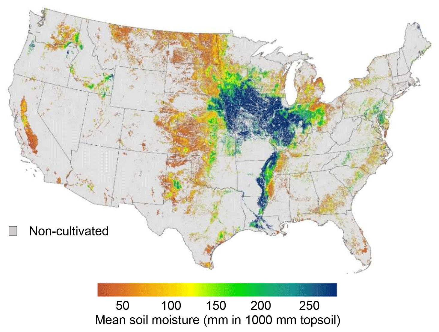
Figure 2Growing season mean soil moisture content (in millimeters in 1000 mm topsoil) as calculated based on daily root zone soil moisture level from April to September for 1981–2015 at 2.5×2.5 arcmin grids, excluding non-cultivated area. The soil moisture level is obtained from the WBM, and non-cultivated area information is from the CDL. This map illustrates the heterogeneity of simulated soil moisture over the continental US and even within states.
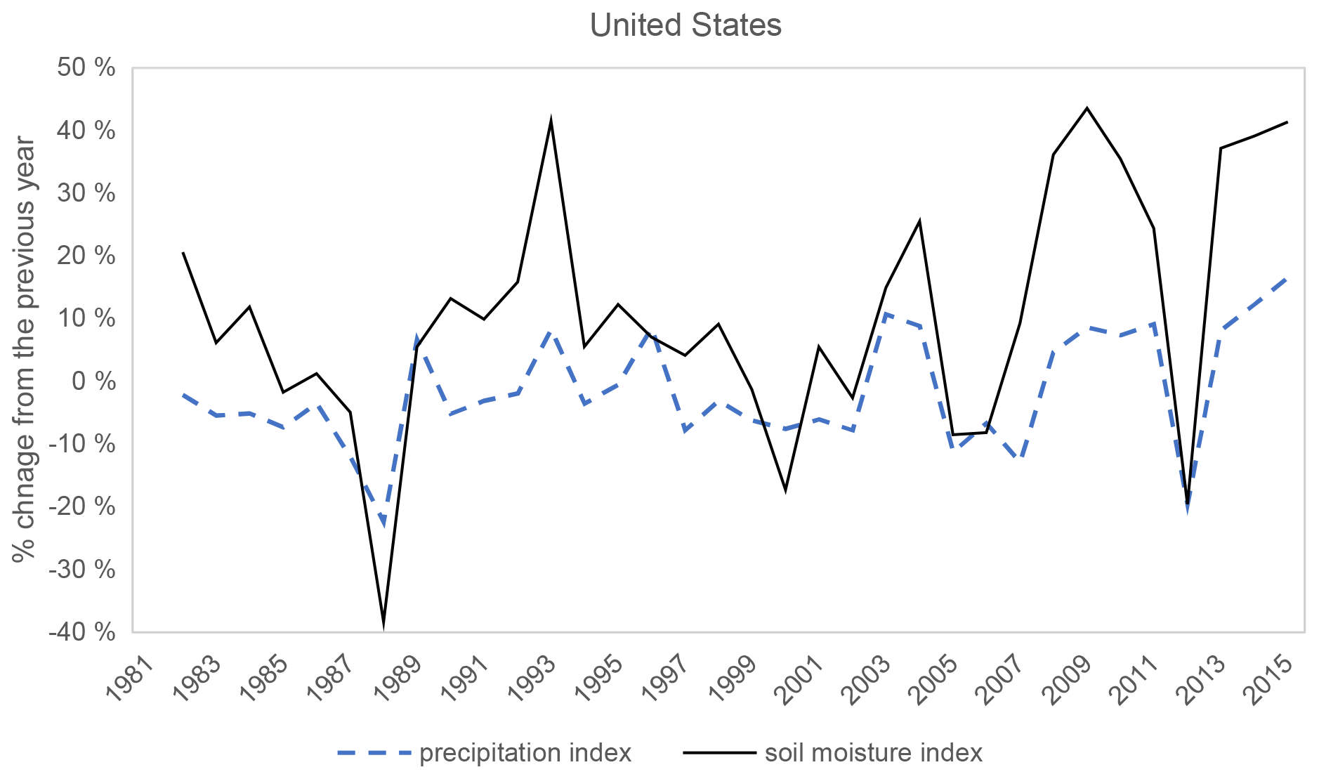
Figure 3Variations in average precipitation versus average soil moisture over corn areas in the United States. The precipitation is aggregated from PRISM, and soil moisture is aggregated from WBM from 2.5 arcmin grid cells weighted by cropland area.
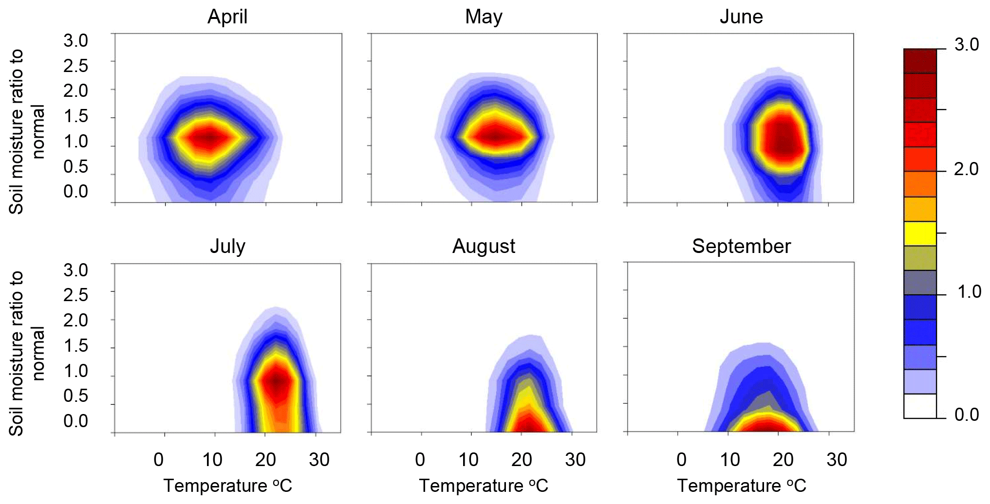
Figure 4The bivariate density of heat and soil moisture for 1981–2015 for all the grid cells in the US Corn Belt. The precipitation is aggregated from PRISM, and soil moisture is aggregated from WBM based on 2.5 arcmin grid cells.
To compare the variation in simulated soil moisture and precipitation, Fig. 3 illustrates the weighted average soil moisture and precipitation over the cultivated US for 1981–2015. In general, variation in soil moisture average is higher than that of precipitation (Fig. 3), showing how this new water metric is different from previous approaches. One interesting finding is that, for some years, the mean precipitation and the mean soil moisture move in opposite directions. For example, in 1990 the mean precipitation is declined by around 5 % while the mean soil moisture is increased by around 13 %.
To show the dynamics of soil moisture and heat, Fig. 4 shows their bivariate distribution by month, based on daily information for all the cultivated grid cells in the US Corn Belt for 1981–2015. Heat and soil moisture combinations vary through the growing season (Fig. 4). The data show significant month-to-month variation, with the second half of the season facing hotter and drier days. Also, July has the highest variation in soil moisture deviation, with a high probability of compound extremes, as the distribution moves toward the lower right.
Below, we describe the regression results from each individual model, and compare their performance to identify which metrics are important to include in the statistical estimate of corn yields. The central finding is that metrics of soil moisture extremes are statistically significant, and models including intensity, duration, and severity metrics (as illustrated in Fig. 1) better capture both the mean and variation in US corn yields. This point is illustrated in Fig. 5, which compares Model (1-a) to Model (2-a) as each model estimates the percentage change in corn yields, assuming additional 10 dday above 29 ∘C and no change in mean soil moisture. Figure 1 shows that Model (1) would significantly underestimate the damage for conditions with extreme water surplus or extreme water deficit.
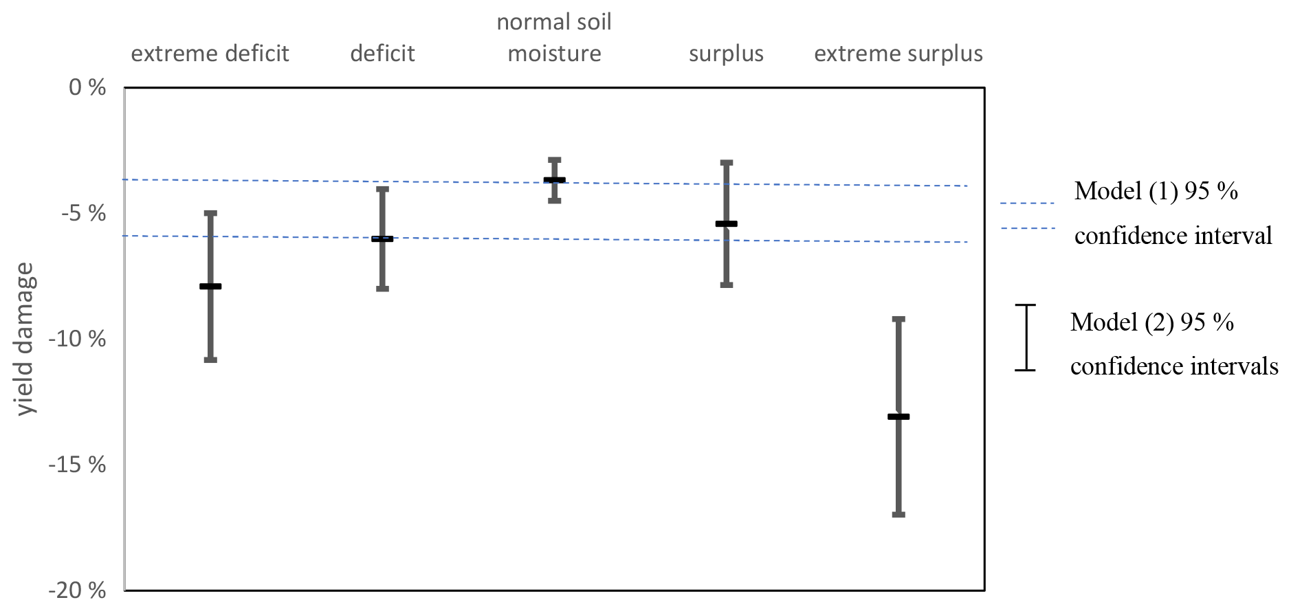
Figure 5Estimated damage to corn yield from additional 10 dday above 29 ∘C and no change in seasonal mean soil moisture.
3.1 Model (1) – predicting yield responses to individual extremes
The results from Model (1-a) show a strong relationship between corn yields and heat and precipitation (Table 2; column 1-a). The marginal impact of dday within 10–29 ∘C is significantly positive, while that from additional dday above 29 ∘C is strongly negative, confirming the seminal findings of Schlenker and Roberts (2009).
Table 2Corn yield estimation without the interaction of heat and soil moisture in Models (1 a–d).
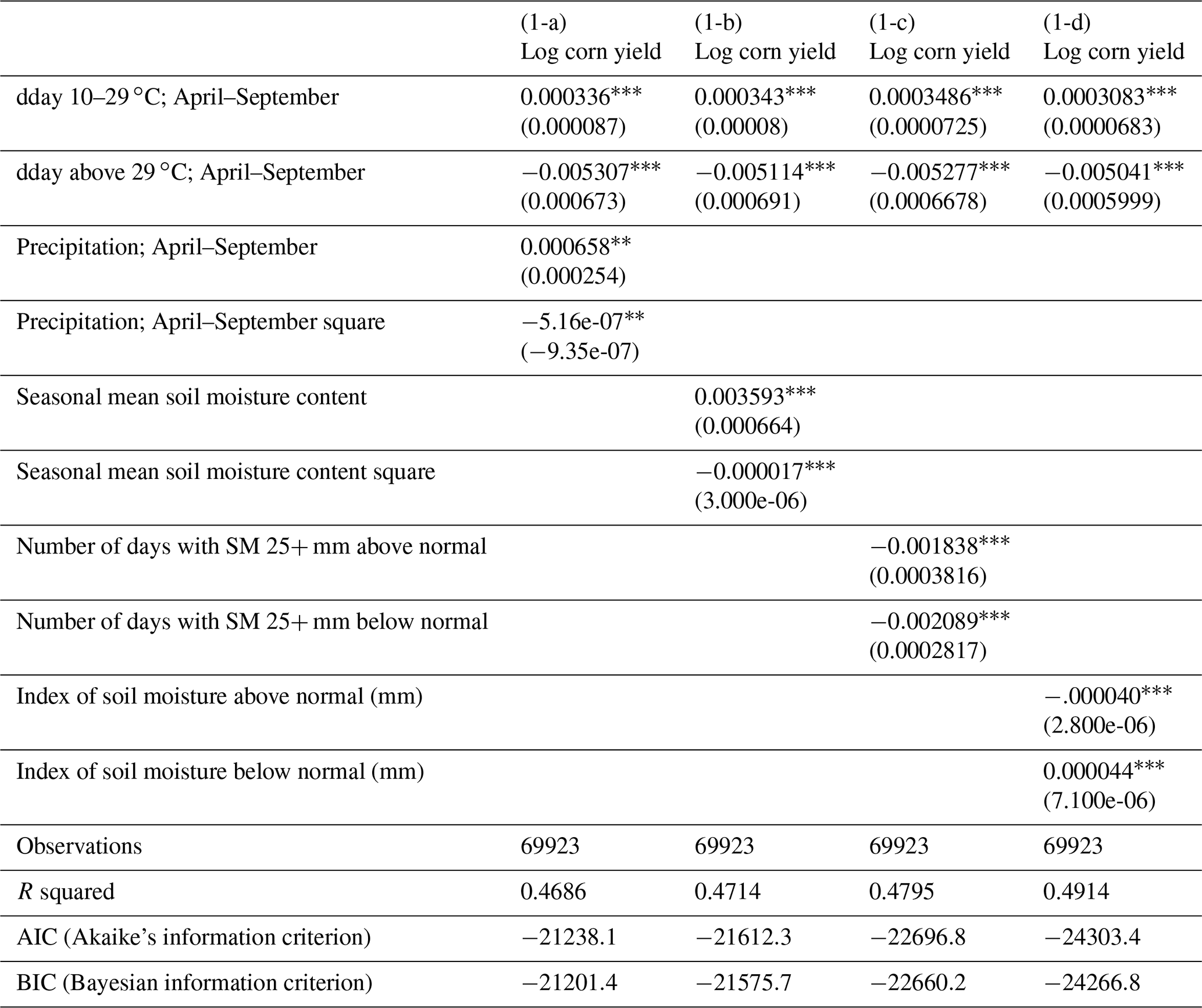
Note: table lists regression coefficients and shows standard errors in parentheses. The constant term and coefficients on the interaction of each state and time trends are not reported. Standard errors are in parentheses and adjusted for state clusters. p<0.01; p<0.05.
The results from Model (1-b), excluding precipitation, show that the marginal relationship with soil moisture is also significant (Table 2; column 1-b). This confirms the findings of Ortiz-Bobea et al. (2019). It shows that the marginal relationship with soil moisture is increasing up to ∼92 in 1000 mm topsoil and decreasing for higher values.
In Model (1-c), we consider the number of days that soil moisture is either too high or too low. The model with metrics of soil moisture extremes further improves the fit, revealing a negative marginal relationship associated with the number of days with low or high soil moisture. Regarding Model (1-c), the coefficient on the number of days with low moisture is also significant and negative. Our estimation sample shows 26 d of high soil moisture and 27 d of low soil moisture on average. The implication is that eliminating 25 d of high soil moisture and 25 d of low soil moisture can improve the corn yields by up to 12.6 %.
Model (1-d) shows the estimated coefficients when considering surplus and deficit (soil moisture deviation from normal) instead of average seasonal soil moisture. Here, we consider two thresholds for low and high soil moisture. Returning to Fig. 1, we evaluate the area of all blue bars and the area of all red bars. It shows that the marginal impact of the moisture deficit (cumulative negative soil moisture deviation) is significant and positive. This indicates the positive contribution of additional soil moisture when the soil moisture levels are below normal. On the other hand, the marginal impact of additional soil moisture in a wet period – i.e., a positive soil moisture deviation – is negative. In other words, this measure captures the fact that plants will benefit from reductions in soil moisture when the soil moisture levels are above normal. This is an indicator of the value of subsurface drainage for agriculture. Note that the Model (1-d) decreases the marginal relationship with extreme heat (dday 29 ∘C). However, this effect is not statistically different from that produced by the first model.
The coefficient of the deficit in Model (1-d) is significant and positive. On the other hand, the coefficient of the extreme deficit is also significant and positive. The estimation sample shows that this metric is around 2300 mm on average. It indicates that reducing the deficit by 2300 mm and reducing the surplus by the same amount can improve the corn yield by up to 21.2 % on average. Note that the mean soil moisture can stay unchanged in this scenario.
3.2 Model (2) – predicting yield responses to compound extremes
In Model (2-a), we introduce heat–soil moisture interactions to test whether soil moisture availability changes the marginal impact of heat on yields (estimation results are in Table 3). We find that the average marginal impacts of dday 29 ∘Cs (heat stress) are all significant. The coefficient on dday 29 ∘C combined with the extreme deficit is −0.0082. The coefficient of dday 29 ∘C (heat stress) combined with extreme water surplus is −0.0140. These figures are significantly different compared to Model (1).
Table 3Corn yield estimation while splitting the heat stress index in Model (2-a).
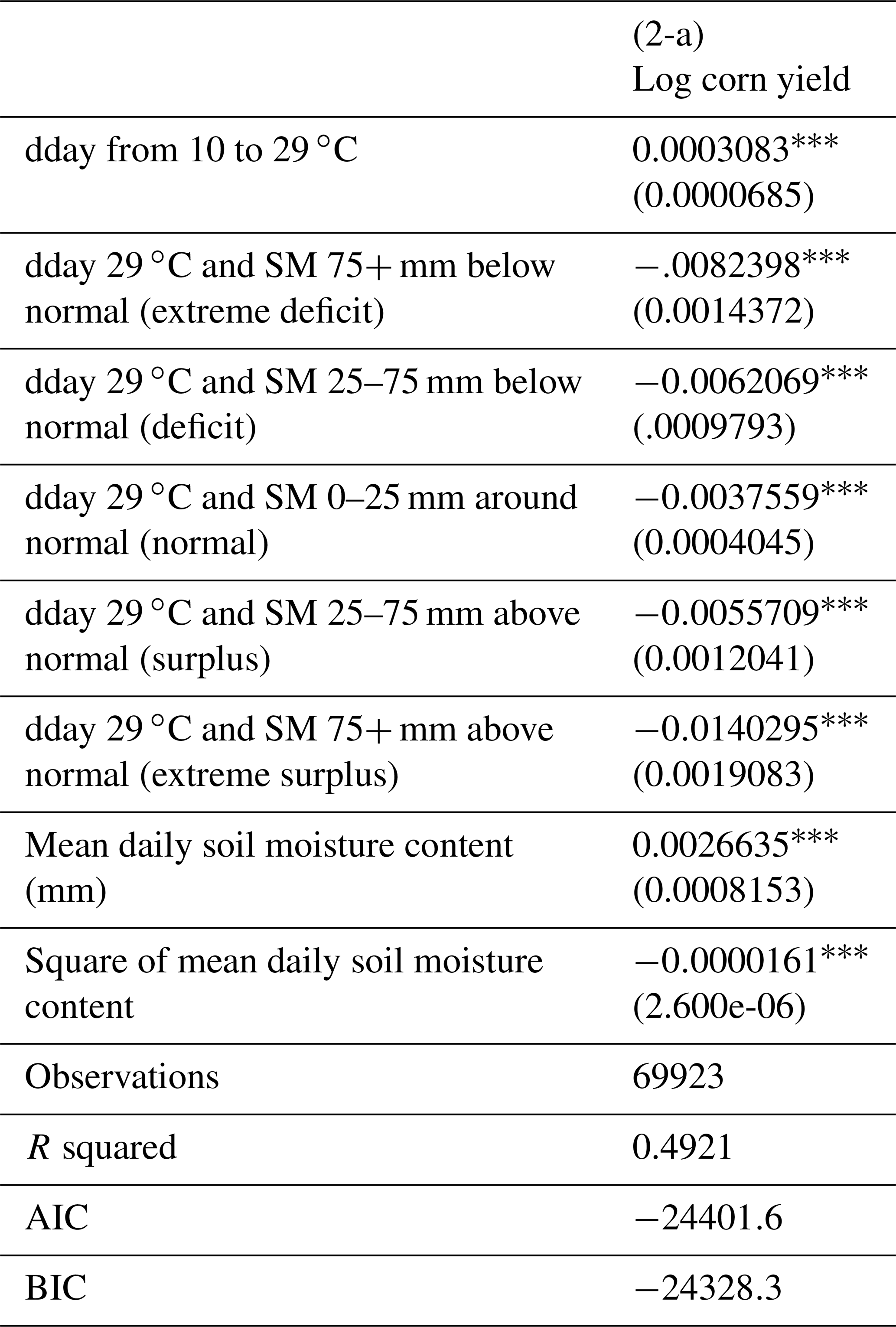
Note: table lists regression coefficients and shows standard errors in parentheses. The constant term and coefficients on the interaction of each state and time trends are not reported. Standard errors are in parentheses and adjusted for state clusters. p<0.01.
We estimate a model with soil moisture while controlling for temperature (Model 2-b). The results are presented in Table 4. The coefficient of dday from 10 to 29 ∘C is significant and positive. This is not significantly different from previous Models (1-a–d) and (2-a). The coefficient on dday above 29 ∘C is significant and negative. It is close to the estimated values from Model (2-a) but slightly lower than Model (1). This indicates that the average damage from extreme heat index (dday 29 ∘C) is around 25 % lower than Model (1). The estimated parameters show the yield response to changes in soil water content. Comparing the parameter values can show the difference in yield response to soil moisture in hot weather and moderate weather. The coefficient on normal soil moisture, conditional to hot weather, is 0.00012. The coefficient on normal soil moisture, conditional to moderate weather, is 0.00003. This indicates that the yield response to water is up to 4 times higher in hot weather. The marginal impact on soil moisture deficit index is 0.00009 in hot weather and is 0.00002 in moderate weather. This also supports the finding that water is up to 4 times more beneficial to corn yields in hot weather. Also, the results show that the damage from excess water is up to 2 times larger in hot weather.
Table 4Estimation of corn yields while splitting the soil moisture metrics in Model (2-b).
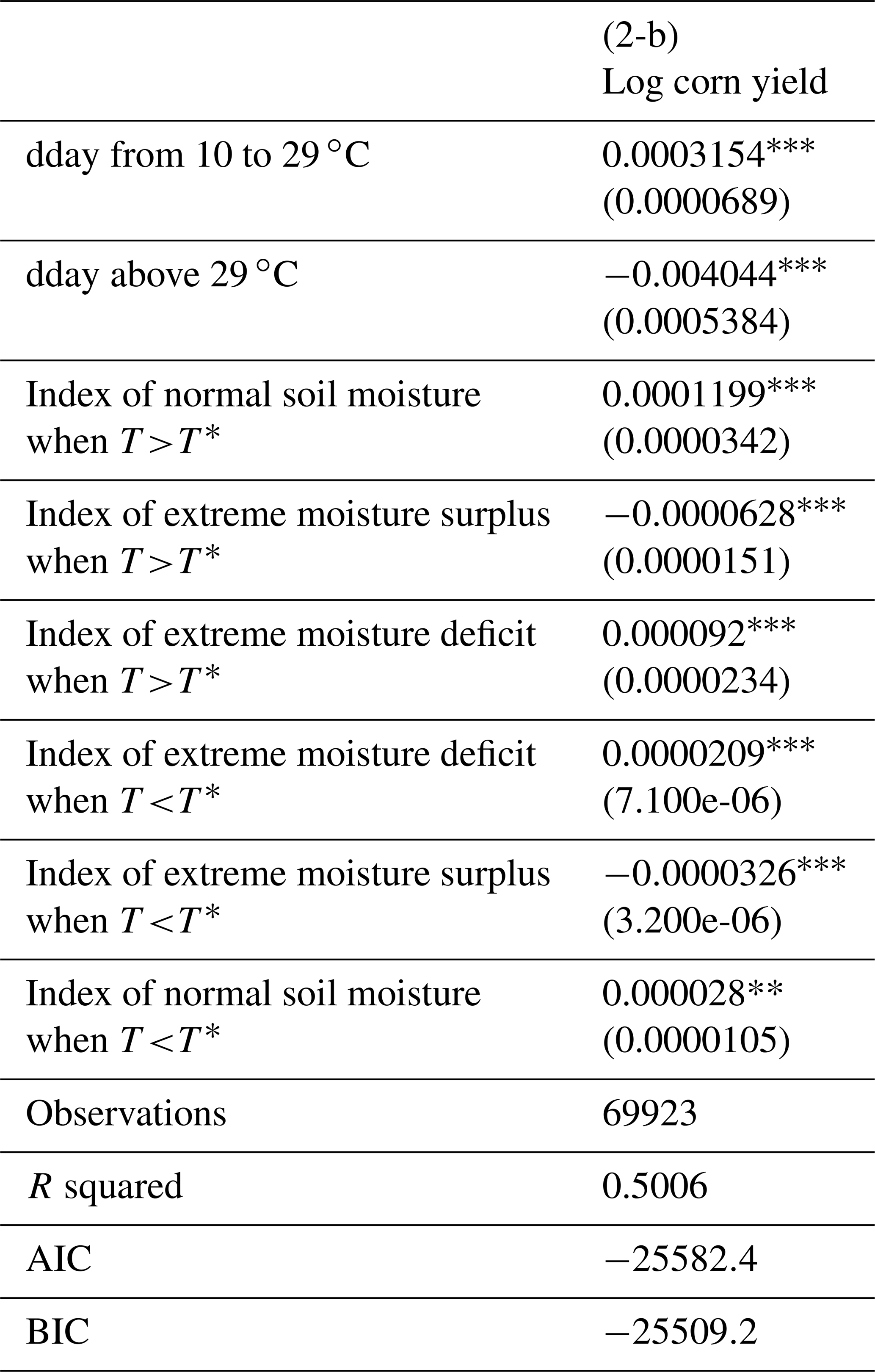
Note: table lists regression coefficients and shows standard errors in parentheses. The constant term and coefficients on the interaction of each state and time trends are not reported. Standard errors are in parenthesis and adjusted for state clusters. p<0.01, p<0.05, * p<0.1.
3.3 Model comparison
A comparison of model performance metrics is given in Table 5, along with a description of the water metric and the extreme metric used in each model. We find that, for Models (1-b–d) and (2-a–d), the coefficients on the soil moisture metrics are significant and with expected signs. Comparing the models' performance suggests that Model (1-b), with mean soil moisture, performs better than the Model (1-a), with cumulative precipitation. Also, Model (1-d), with the extreme soil moisture metrics, outperforms both previous models (with cumulative precipitation or with mean soil moisture). The best corn yield predictor is from Models (2-a) and (2-b), considering compound extremes through the daily interaction of heat and soil moisture. We find that using a seasonally averaged soil moisture metric is insufficient for capturing yield extremes; i.e., the temporal resolution of the soil moisture metric is important for estimating corn yield variability. Figure 6 illustrates the difference by comparing the modeled impacts of average soil moisture (Model 1-b) on corn yields (Fig. 6a) to the impacts, considering the deviation from normal soil moisture (Model 1-d) estimated for a sandy soil type (Fig. 6b) and a clay soil type (Fig. 6c). In other words, when parametrizing the soil moisture as a deviation from normal, we obtain a specific piecewise linear yield response to water, depending on soil types (and normal levels of soil moisture), the extremes of which are completely missed by the model as it only uses mean soil moisture. We find that the average corn yield damage from excess heat is up to 4 times more severe when combined with water stress. This damage can only be estimated when including soil moisture and metrics of extreme water stress (e.g., Models 2-a–d).
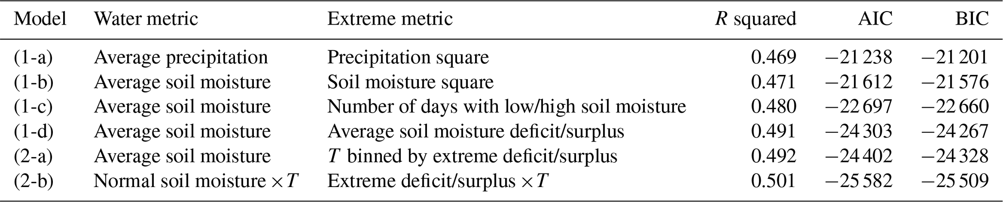
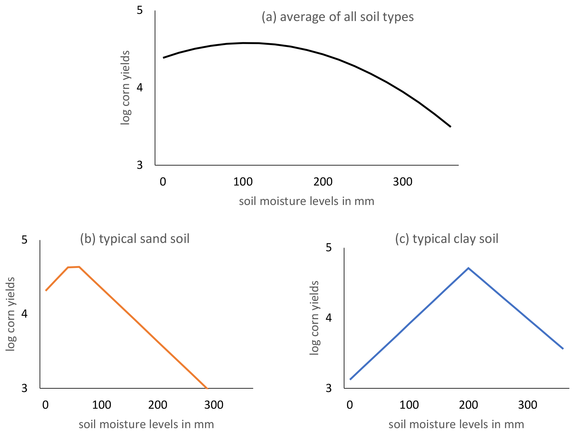
Figure 6Estimated impact of soil moisture on log corn yields. Including soil moisture in the regression and its square term, as in Model (1-b), will give us a quadratic relationship between soil moisture and yields, as seen in (a). A piecewise linear parametrization, as in Model (1-d), can provide the location-specific piecewise linear relationship based on soil moisture deviation from normal, as seen in (b) and (c). This will cause the maximum of the response curve to be in lower soil moisture levels for sand and in higher soil moisture levels for clay soil texture.
3.4 Decomposing the variation in US corn yields
We have decomposed the changes in the US corn yields from 1981 to 2015 to understand the relative roles of soil moisture and heat in interannual corn yield variation. Figure 7 illustrates a decomposition based on our findings, which are aggregated for the whole US. With no climate variation, the US corn yield is expected to have a smooth positive trend, as shown in green. The deviation from the trend occurs due to changes in water and heat stressors. The blue bars show the expected changes in US corn yields due to changes in the water stress, while the orange bars demonstrate the expected yield changes due to changes in heat stress. While there have been years in which the stressors have moved together (e.g., 2011 and 2012), for several years water and heat have offset each other's benefit or damage. For example, in 1992 the damage from heat is partially offset by benefits from water, or in 2010, the damage from water stress is partially offset by benefits from heat.
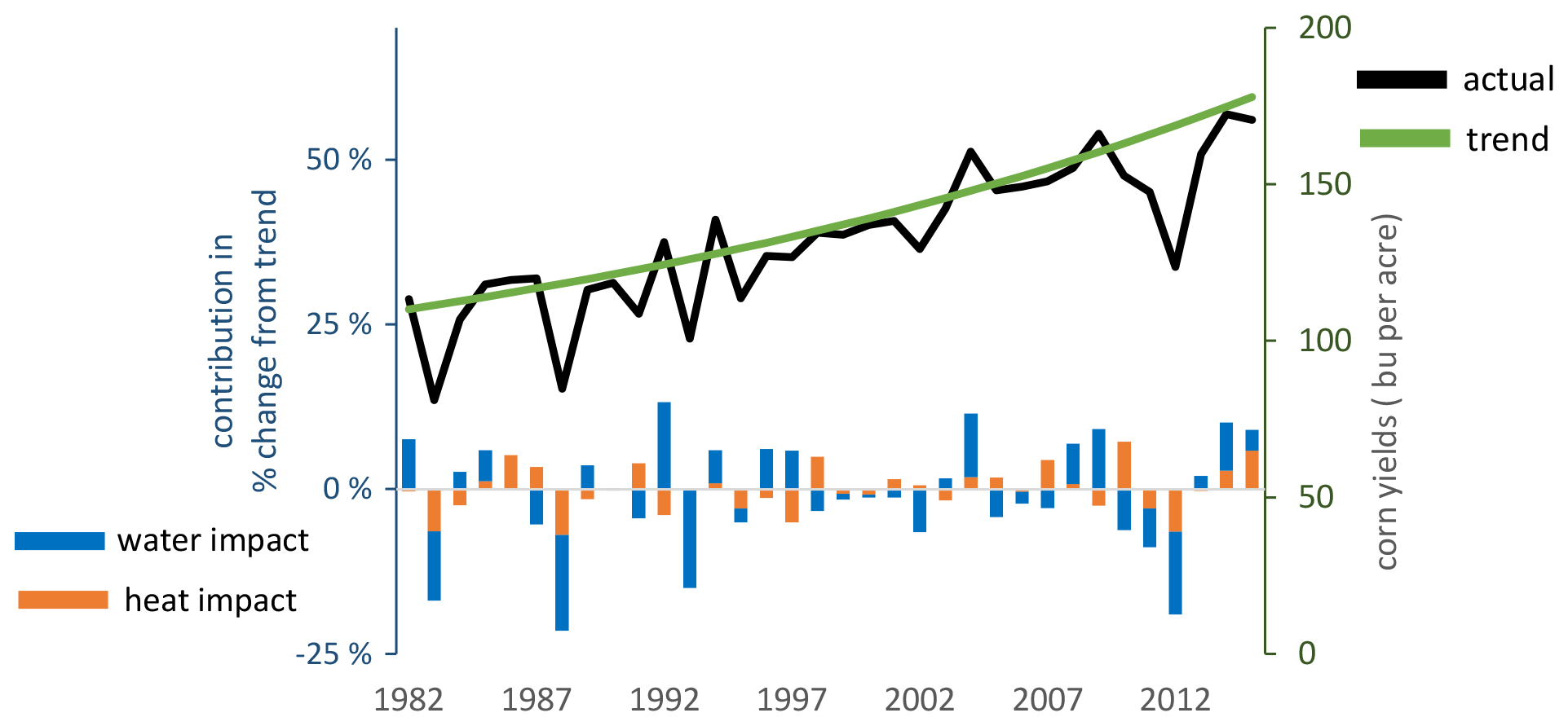
Figure 7The bars show the contribution of water and contribution of heat in variation in the US corn yields (left axis). The lines illustrate actual yields and trend (right axis).
3.5 Robustness checks
The Supplement provides several robustness checks. The goal is to investigate whether different assumptions can improve the predictive power of Model (1) such that it outperforms Model (2). We answer three questions. First, are the estimation results from Model (1) different from those using alternative water metrics from WBM output? Second, are the estimates in Model (1) different from those obtained using a model considering growth stages? And third, do the main findings change if we alter the geographical scope of the study?
For the first robustness question, i.e., alternative water metrics, we re-estimate Model (1) using daily evapotranspiration (which is related to the water requirements of plants) and soil moisture fraction. Overall, the findings remain robust to alternative soil moisture metrics from WBM, including the mean of soil moisture fraction (soil moisture content divided by field capacity), the seasonal mean of evapotranspiration and within-season standard deviations of them. We also look at the results using an alternative interpolation of WBM data to PRISM resolution (nearest neighbor versus bilinear interpolations). We reject the null hypothesis that the coefficient on yield response to heat is different between these two metrics. Also, we reject the null hypothesis that the prediction power across these models is higher than Model (2).
To test the second robustness question, i.e., time separability, we re-estimate Model (1-b) for 2-month intervals (April–May, June–July, and August–September), and the findings remain robust. We find that considering bimonthly variables does not change the yield response to heat. Although this alternative formulation does improve the predictive power of Model (1-b) a little bit, the performance is not better than the original Models (2-a) and (2-b) with compound extremes.
To test the sensitivity of our findings to geographical area, we re-estimate the models for eastern US and western US. We find that the estimated coefficients of Models (1-a) and (1-b) are not robust to the geographical choice, while those of Model (2) remain robust.
In this paper, we have identified new water availability metrics that improve the predictive power of statistical corn yield models. While predictive power is an important outcome of this analysis, the insights gained from incrementally adding higher temporal-resolution metrics of water extremes to the models are also valuable for understanding the drivers of corn yield variability and for revealing the resolution of water availability data required to capture future extremes under climate change scenarios. Statistical crop models have been used to both elucidate drivers of crop yield trends and variability and to evaluate potential climate change impacts on crop production in the future (e.g., Lobell and Burke, 2010; Diffenbaugh et al., 2012). However, these models typically use seasonally averaged water availability metrics (e.g., total growing season precipitation) and utilize precipitation more often than soil moisture. Generally, if the location of the study does not expect a significant change in the within-season distribution of the soil moisture, a mean soil moisture index will work. However, if there is an expected change in this distribution, using the mean variable will create biased yield projections. Because climate models project significant changes in the frequency and intensity of both extreme precipitation and temperature (Bevacqua et al., 2019; Manning et al., 2019; Myhre et al., 2019; Poschlod et al., 2020; Potopová et al., 2020; Wehner, 2019; Zscheischler et al., 2018), the results presented here show that the mean metrics of water availability – especially mean precipitation – are not sufficient for capturing the impacts on yields. It is necessary to consider the metrics of extreme events as illustrated in Fig. 1. As we find that the coefficient on extreme heat is significantly different when considering soil moisture, it is possible that previous climate impact studies have over- or underestimated the yield impacts. Furthermore, farm management practices can alter soil moisture – and therefore yields – independent of precipitation. Supplemental irrigation, and no-till farming, cover cropping, and soil conservation, can increase soil moisture. These adaptations may occur in places predicted to face higher mean precipitation coupled with more extreme water events. The results of these management practices cannot be captured by statistical models looking at precipitation metrics alone. Such precipitation-based studies could potentially lead to overestimation yield damages under future climate extremes by not accounting for human adaptations designed to conserve soil moisture.
Applying this framework to climate impact studies will face a key challenge, namely projecting the future compound extremes with the high temporal resolution of Model (2). It requires collaboration between hydrologists, climate scientists, and statisticians (Zscheischler et al., 2020). For future yield projections, we need reliable future projections of daily temperature (maximum and minimum) and soil moisture. Unfortunately, to the best of our knowledge, available data sets including predictions of future soil moisture have a relatively coarse spatial and temporal resolution and rely on climate model projections with known difficulties to represent daily temporal-resolution events (Hempel et al., 2013). Further research is required to improve the ability of climate models and impact models to project the bivariate distribution of heat–moisture (Sarhadi et al., 2018).
This study serves to bridge the gap between statistical studies of climate impacts on crops and their biophysical counterparts by recognizing the central role of soil moisture – which is not a simple linear transformation of precipitation – in understanding crop yields. We employ a fine-scale, high temporal-resolution data set to investigate the conditional marginal value of soil moisture and heat in US corn yields for the 1981–2015 period employing a statistical framework. The major contribution of this study is showing that the coefficient on extreme heat (dday 29 ∘C) is significantly different, while considering daily interactions with soil moisture, emphasizing the importance of compound hydroclimatic conditions.
Our first key finding is that seasonal mean soil moisture performs better than average precipitation in statistically predicting corn yield. While the majority of current empirical studies employ precipitation as a proxy of water availability for crops, we show that the precipitation coefficient may not be always an appropriate measure of water availability. This study suggests that soil moisture content should be used for estimating crop yields instead of cumulative rainfall for locations with high runoff, drainage, or irrigation (e.g., western and central US).
Also, the metrics of soil moisture extremes can explain a portion of the damages to corn yield. On average, farmers can improve corn yields by up to 24 % only by avoiding extreme water stress. We also find that the coefficient of excess soil moisture is negative. This is in line with the current agronomic literature (Torbert et al., 1993; Urban et al., 2015) which points out that high soil moisture content can result in nutrient loss through excess water flows. In addition, at high humidity, the plants may have difficulty remaining cool at high temperatures. There is also a risk of waterlogging soils. With a few notable exceptions (e.g., rice), most crops do not grow well in inundated conditions as the plant roots need oxygen, so the direct impact of excess water stress is because of the anoxic conditions.
Finally, the marginal impact of the heat index on crop yields depends on the soil moisture level. We show that the average yield damage from heat stress is up to 4 times more severe when combined with water stress; therefore, the value of water in maintaining crop yield is up to 4 times larger on hot days.
The codes are available at https://doi.org/10.4231/Q07D-J369 (Haqiqi et al., 2020a).
The historical weather data (PRISM) are available at http://www.prism.oregonstate.edu (PRISM Climate Group, 2019). The input data for estimations are available at https://doi.org/10.4231/0M14-EY38 (Haqiqi et al., 2020b).
The supplement related to this article is available online at: https://doi.org/10.5194/hess-25-551-2021-supplement.
All authors contributed to the conceptualization, methodology, formal analysis, and reviewing and editing of the paper. IH and DSG collected model input, performed the simulations, and contributed to the investigation, resources, software, and validation. IH contributed to writing the original draft and visualization. TWH assisted with the supervision and contributed to the funding acquisition.
The authors declare that they have no conflict of interest.
This article is part of the special issue “Understanding compound weather and climate events and related impacts (BG/ESD/HESS/NHESS inter-journal SI)”. It is not associated with a conference.
The database construction process was done by employing the high-performance computing solutions of the Institute for CyberScience Advanced CyberInfrastructure (ICS-ACI) at the Pennsylvania State University.
This work was supported by the US Department of Energy, Office of Science, Biological and Environmental Research program, Earth and Environmental Systems Modeling, MultiSector Dynamics (contract no. DE-SC0016162).
This paper was edited by Bart van den Hurk and reviewed by two anonymous referees.
Bevacqua, E., Maraun, D., Vousdoukas, M. I., Voukouvalas, E., Vrac, M., Mentaschi, L., and Widmann, M.: Higher probability of compound flooding from precipitation and storm surge in Europe under anthropogenic climate change, Sci. Adv., 5, eaaw5531, https://doi.org/10.1126/sciadv.aaw5531, 2019.
Boryan, C., Yang, Z., and Di, L.: Deriving 2011 cultivated land cover data sets using usda national agricultural statistics service historic cropland data layers, Proc. of IEEE International Geoscience and Remote Sensing Symposium, 22–27 July 2012, Munich, Germany, 6297–6300, 2012.
Bradford, J. B., Schlaepfer, D. R., Lauenroth, W. K., Yackulic, C. B., Duniway, M., Hall, S., Jia, G., Jamiyansharav, K., Munson, S. M., Wilson, S. D., and Tietjen, B.: Future soil moisture and temperature extremes imply expanding suitability for rainfed agriculture in temperate drylands, Sci. Rep.-UK, 7, 12923, https://doi.org/10.1038/s41598-017-13165-x, 2017.
Burke, M. and Emerick, K.: Adaptation to climate change: Evidence from US agriculture, Am. Econ. J. Econ. Policy, 8, 106–140, 2016.
Comas, L. H., Trout, T. J., DeJonge, K. C., Zhang, H., and Gleason, S. M.: Water productivity under strategic growth stage-based deficit irrigation in maize, Agric. Water Manag., 212, 433–440, https://doi.org/10.1016/j.agwat.2018.07.015, 2019.
D'Agostino, A. L. and Schlenker, W.: Recent weather fluctuations and agricultural yields: implications for climate change, Agr. Econ., 47, 159–171, https://doi.org/10.1111/agec.12315, 2016.
Denmead, O. T. and Shaw, R. H.: The Effects of Soil Moisture Stress at Different Stages of Growth on the Development and Yield of Corn 1, Agron. J., 52, 272–274, https://doi.org/10.2134/agronj1960.00021962005200050010x, 1960.
Diffenbaugh, N. S., Hertel, T. W., Scherer, M., and Verma, M.: Response of corn markets to climate volatility under alternative energy futures, Nat. Clim. Change, 2, 514–518, https://doi.org/10.1038/nclimate1491, 2012.
D'Odorico, P. and Porporato, A.: Preferential states in soil moisture and climate dynamics, PNAS, 101, 8848–8851, https://doi.org/10.1073/pnas.0401428101, 2004.
Fishman, R.: More uneven distributions overturn benefits of higher precipitation for crop yields, Environ. Res. Lett., 11, 024004, https://doi.org/10.1088/1748-9326/11/2/024004, 2016.
Grogan, D.: Global and regional assessments of unsustainable groundwater use in irrigated agriculture, PhD thesis, University of New Hampshire, Durham, US, available at: https://scholars.unh.edu/dissertation/2 (last access: 15 January 2018), 2016.
Haqiqi, I., Grogan, D. S., Hertel, T. W., and Schlenker, W.: Model Code for: Quantifying the Impacts of Compound Extremes on Agriculture and Irrigation Water Demand, https://doi.org/10.4231/Q07D-J369, 2020a.
Haqiqi, I., Grogan, D. S., Hertel, T. W., and Schlenker, W.: Model Code for: Quantifying the Impacts of Compound Extremes on Agriculture and Irrigation Water Demand, https://doi.org/10.4231/0M14-EY38, 2020b.
Hauser, M., Thiery, W., and Seneviratne, S. I.: Potential of global land water recycling to mitigate local temperature extremes, Earth Syst. Dynam., 10, 157–169, https://doi.org/10.5194/esd-10-157-2019, 2019.
Hempel, S., Frieler, K., Warszawski, L., Schewe, J., and Piontek, F.: A trend-preserving bias correction – the ISI-MIP approach, Earth Syst. Dynam., 4, 219–236, https://doi.org/10.5194/esd-4-219-2013, 2013.
Jones, J. W., Antle, J. M., Basso, B., Boote, K. J., Conant, R. T., Foster, I., Godfray, H. C. J., Herrero, M., Howitt, R. E., and Janssen, S.: Brief history of agricultural systems modeling, Agric. Syst., 155, 240–254, 2017.
Kaur, G., Nelson, K. A., and Motavalli, P. P.: Early-Season Soil Waterlogging and N Fertilizer Sources Impacts on Corn N Uptake and Apparent N Recovery Efficiency, Agronomy, 8, 102, https://doi.org/10.3390/agronomy8070102, 2018.
Li, G., Zhao, B., Dong, S., Zhang, J., Liu, P., and Vyn, T. J.: Impact of controlled release urea on maize yield and nitrogen use efficiency under different water conditions, Plos One, 12, e0181774, https://doi.org/10.1371/journal.pone.0181774, 2017.
Liu, B., Asseng, S., Müller, C., Ewert, F., Elliott, J., Lobell, D. B., Martre, P., Ruane, A. C., Wallach, D., and Jones, J. W.: Similar estimates of temperature impacts on global wheat yield by three independent methods, Nat. Clim. Change, 6, 1130–1136, 2016.
Lobell, D. B. and Burke, M. B.: On the use of statistical models to predict crop yield responses to climate change, Agr. Forest Meteorol., 150, 1443–1452, https://doi.org/10.1016/j.agrformet.2010.07.008, 2010.
Lobell, D. B., Hammer, G. L., McLean, G., Messina, C., Roberts, M. J., and Schlenker, W.: The critical role of extreme heat for maize production in the United States, Nat. Clim. Change, 3, 497–501, https://doi.org/10.1038/nclimate1832, 2013.
Manning, C., Widmann, M., Bevacqua, E., Loon, A. F. V., Maraun, D., and Vrac, M.: Increased probability of compound long-duration dry and hot events in Europe during summer (1950–2013), Environ. Res. Lett., 14, 094006, https://doi.org/10.1088/1748-9326/ab23bf, 2019.
McDonald, R. I. and Girvetz, E. H.: Two Challenges for U.S. Irrigation Due to Climate Change: Increasing Irrigated Area in Wet States and Increasing Irrigation Rates in Dry States, Plos One, 8, e65589, https://doi.org/10.1371/journal.pone.0065589, 2013.
Meng, Q., Chen, X., Lobell, D. B., Cui, Z., Zhang, Y., Yang, H., and Zhang, F.: Growing sensitivity of maize to water scarcity under climate change, Sci. Rep.-UK, 6, 19605, https://doi.org/10.1038/srep19605, 2016.
Myhre, G., Alterskjær, K., Stjern, C. W., Hodnebrog, Ø., Marelle, L., Samset, B. H., Sillmann, J., Schaller, N., Fischer, E., Schulz, M., and Stohl, A.: Frequency of extreme precipitation increases extensively with event rareness under global warming, Sci. Rep.-UK, 9, 1–10, https://doi.org/10.1038/s41598-019-52277-4, 2019.
Ortiz-Bobea, A., Wang, H., Carrillo, C. M., and Ault, T. R.: Unpacking the climatic drivers of US agricultural yields, Environ. Res. Lett., 14, 064003, https://doi.org/10.1088/1748-9326/ab1e75, 2019.
Peichl, M., Thober, S., Meyer, V., and Samaniego, L.: The effect of soil moisture anomalies on maize yield in Germany, Nat. Hazards Earth Syst. Sci., 18, 889–906, https://doi.org/10.5194/nhess-18-889-2018, 2018.
Poschlod, B., Zscheischler, J., Sillmann, J., Wood, R. R., and Ludwig, R.: Climate change effects on hydrometeorological compound events over southern Norway, Weather Clim. Extrem., 28, 100253, https://doi.org/10.1016/j.wace.2020.100253, 2020.
Potopová, V., Trnka, M., Hamouz, P., Soukup, J., and Castraveț, T.: Statistical modelling of drought-related yield losses using soil moisture-vegetation remote sensing and multiscalar indices in the south-eastern Europe, Agric. Water Manag., 236, 106168, https://doi.org/10.1016/j.agwat.2020.106168, 2020.
PRISM Climate Group: Parameter-elevation Regressions on Independent Slopes Model, Oregon State University, available at: http://prism.oregonstate.edu, last access: 15 January 2019.
Ribeiro, A. F. S., Russo, A., Gouveia, C. M., Páscoa, P., and Zscheischler, J.: Risk of crop failure due to compound dry and hot extremes estimated with nested copulas, Biogeosciences, 17, 4815–4830, https://doi.org/10.5194/bg-17-4815-2020, 2020.
Rippey, B. R.: The US drought of 2012, Weather Clim. Extrem., 10, 57–64, 2015.
Rizzo, G., Edreira, J. I. R., Archontoulis, S. V., Yang, H. S., and Grassini, P.: Do shallow water tables contribute to high and stable maize yields in the US Corn Belt?, Glob. Food Secur., 18, 27–34, https://doi.org/10.1016/j.gfs.2018.07.002, 2018.
Roberts, M. J., Schlenker, W., and Eyer, J.: Agronomic Weather Measures in Econometric Models of Crop Yield with Implications for Climate Change, Am. J. Agric. Econ., 95, 236–243, https://doi.org/10.1093/ajae/aas047, 2013.
Sarhadi, A., Ausín, M. C., Wiper, M. P., Touma, D., and Diffenbaugh, N. S.: Multidimensional risk in a nonstationary climate: Joint probability of increasingly severe warm and dry conditions, Sci. Adv., 4, eaau3487, https://doi.org/10.1126/sciadv.aau3487, 2018.
Schaffer, B. E., Nordbotten, J. M., and Rodriguez-Iturbe, I.: Plant biomass and soil moisture dynamics: analytical results, Proc. R. Soc. A, 471, 20150179, https://doi.org/10.1098/rspa.2015.0179, 2015.
Schlenker, W. and Roberts, M. J.: Nonlinear temperature effects indicate severe damages to US crop yields under climate change, P. Natl. Acad. Sci. USA, 106, 15594–15598, 2009.
Schmidt, J. P., Sripada, R. P., Beegle, D. B., Rotz, C. A., and Hong, N.: Within-Field Variability in Optimum Nitrogen Rate for Corn Linked to Soil Moisture Availability, Soil Sci. Soc. Am. J., 75, 306–316, https://doi.org/10.2136/sssaj2010.0184, 2011.
Siebert, S., Webber, H., Zhao, G., and Ewert, F.: Heat stress is overestimated in climate impact studies for irrigated agriculture, Environ. Res. Lett., 12, 054023, https://doi.org/10.1088/1748-9326/aa702f, 2017.
Tebaldi, C. and Lobell, D.: Differences, or lack thereof, in wheat and maize yields under three low-warming scenarios, Environ. Res. Lett., 13, 065001, https://doi.org/10.1088/1748-9326/aaba48, 2018.
Torbert, H. A., Hoeft, R. G., Vanden Heuvel, R. M., Mulvaney, R. L., and Hollinger, S. E.: Short-term excess water impact on corn yield and nitrogen recovery, J. Prod. Agric., 6, 337–344, 1993.
Urban, D., Roberts, M. J., Schlenker, W., and Lobell, D. B.: Projected temperature changes indicate significant increase in interannual variability of U.S. maize yields, Clim. Change, 112, 525–533, https://doi.org/10.1007/s10584-012-0428-2, 2012.
Urban, D. W., Roberts, M. J., Schlenker, W., and Lobell, D. B.: The effects of extremely wet planting conditions on maize and soybean yields, Clim. Change, 130, 247–260, https://doi.org/10.1007/s10584-015-1362-x, 2015.
USDA-NASS: USDA-National Agricultural Statistics Service, Cropland Data Layer, U. S. Dep. Agric. Natl. Agric. Stat. Serv. Mark. Inf. Serv. Off. Wash. DC, available at: https://www.nass.usda.gov/Research_and_Science/Cropland/Release/ (last access: 15 January 2021), 2017.
Wang, R., Bowling, L. C., Cherkauer, K. A., Cibin, R., Her, Y., and Chaubey, I.: Biophysical and hydrological effects of future climate change including trends in CO2, in the St. Joseph River watershed, Eastern Corn Belt, Agric. Water Manag., 180, 280–296, https://doi.org/10.1016/j.agwat.2016.09.017, 2017.
Wehner, M.: Estimating the probability of multi-variate extreme weather events, in: Workshop on Correlated Extremes, Columbia University, New York, USA, May 2019.
Werner, A. T. and Cannon, A. J.: Hydrologic extremes – an intercomparison of multiple gridded statistical downscaling methods, Hydrol. Earth Syst. Sci., 20, 1483–1508, https://doi.org/10.5194/hess-20-1483-2016, 2016.
Williams, A., Hunter, M. C., Kammerer, M., Kane, D. A., Jordan, N. R., Mortensen, D. A., Smith, R. G., Snapp, S., and Davis, A. S.: Soil Water Holding Capacity Mitigates Downside Risk and Volatility in US Rainfed Maize: Time to Invest in Soil Organic Matter?, Plos One, 11, e0160974, https://doi.org/10.1371/journal.pone.0160974, 2016.
Wing, I. S., Monier, E., Stern, A., and Mundra, A.: US major crops' uncertain climate change risks and greenhouse gas mitigation benefits, Environ. Res. Lett., 10, 115002, https://doi.org/10.1088/1748-9326/10/11/115002, 2015.
Wisser, D., Fekete, B. M., Vörösmarty, C. J., and Schumann, A. H.: Reconstructing 20th century global hydrography: a contribution to the Global Terrestrial Network- Hydrology (GTN-H), Hydrol. Earth Syst. Sci., 14, 1–24, https://doi.org/10.5194/hess-14-1-2010, 2010.
WMO: The global climate 2001–2010: A decade of climate extremes, WMO-No 1103, 119, World Meteorological Organization (WMO), Geneva, Switzerland, 2013.
Zscheischler, J., Westra, S., Van Den Hurk, B. J., Seneviratne, S. I., Ward, P. J., Pitman, A., AghaKouchak, A., Bresch, D. N., Leonard, M., and Wahl, T.: Future climate risk from compound events, Nat. Clim. Change, 8, 469–477, 2018.
Zscheischler, J., van den Hurk, B., Ward, P. J., and Westra, S.: Multivariate extremes and compound events, in: Climate Extremes and Their Implications for Impact and Risk Assessment, Elsevier, the Netherlands, 59–76, https://doi.org/10.1016/C2017-0-01794-9, 2020.