Hysteresis in soil hydraulic conductivity as driven by salinity and sodicity – a modeling framework

Declining soil-saturated hydraulic conductivity (K_s) as a result of saline and sodic irrigation water is a major cause of soil degradation. While it is understood that the mechanisms that lead to degradation can cause irreversible changes in K_s, existing models do not account for hysteresis between the degradation and rehabilitation processes. We develop the first model for the effect of saline and sodic water on K_s that explicitly includes hysteresis. As such, the idea that a soil's history of degradation and rehabilitation determines its future K_s lies at the center of this model. By means of a “weight” function, the model accounts for soil-specific differences, such as clay content. The weight function also determines the form of the hysteresis curves, which are not restricted to a single shape, as in some existing models for irreversible soil processes. The concept of the weight function is used to develop a reversibility index, which allows for the quantitative comparison of different soils and their susceptibility to irreversible degradation. We discuss the experimental setup required to find a soil's weight function and show how the weight function determines the degree to which K_s is reversible for a given soil. We demonstrate the feasibility of this procedure by presenting experimental results showcasing the presence of hysteresis in soil K_s and using these results to calculate a weight function. Past experiments and models on the decline of K_s due to salinity and sodicity focus on degradation alone, ignoring any characterization of the degree to which declines in K_s are reversible. Our model and experimental results emphasize the need to measure “reversal curves”, which are obtained from rehabilitation measurements following mild declines in K_s. The developed model has the potential to significantly improve our ability to assess the risk of soil degradation by allowing for the consideration of how the accumulation of small degradation events can cause significant land degradation.

1 Introduction

Soil degradation caused by the use of saline and sodic irrigation water is a major threat to agricultural production and food security. Each year, as much as 1.5 million ha of farmland are irretrievably lost due to salinity- and sodicity-induced degradation, while crop output is decreased on an additional 20 to 46 million ha (FAO and ITPS, 2015). Together, this results in widespread economic losses and declines in production that elevate stress on food supplies (Qadir et al., 2014). Growing strain on freshwater resources, rising human populations, and climate change are all likely to increase reliance on saline and sodic irrigation water to support food production, further raising the risk of debilitating soil degradation in the near future.

In this paper, we focus on changes to saturated hydraulic conductivity, K_s, as the major indicator of soil degradation (McNeal and Coleman, 1966; Yaron and Thomas, 1968; Chen and Banin, 1975; Shainberg and Singer, 2011; Hillel, 2000). Saline and sodic conditions cause declines in K_s through a combination of different soil processes, including clay swelling, clay dispersion, and slaking. While swelling is usually considered to be a reversible process, clay dispersion is thought to cause irreversible changes in the soil matrix and, thus, K_s (Quirk and Schofield, 1955; McNeal and Coleman, 1966; Chen and Banin, 1975; Ezlit et al., 2013; Dang et al., 2018a, b). No clear dividing line exists, however, between the onset of swelling and dispersion, and experimental studies have shown that declines in K_s are characterized by smooth curves as water quality is changed, rather than by abrupt jumps (Quirk and Schofield, 1955; McNeal and Coleman, 1966; Chen and Banin, 1975). We hypothesize that this smooth behavior is due to soil heterogeneity, with different aggregates exhibiting different thresholds between swelling and dispersion, and the overall behavior of the soil corresponding to the integrated response of all aggregates. This point constitutes a cornerstone of the framework upon which our model lies, and we will return to it during the model development.

While numerous experimental studies have led to models describing declines in K_s due to salinity and sodicity, we are unaware of any model that considers differences between degradation and rehabilitation (McNeal and Coleman, 1966; McNeal, 1968; Yaron and Thomas, 1968; Lagerwerff et al., 1969; Russo, 1988; Ezlit et al., 2013; Ali et al., 2019). That is, all existing models assume that these two processes are strictly reversible, meaning decreases in K_s can be restored simply by changing the chemical properties of the soil water (McNeal and Coleman, 1966; McNeal, 1968; Yaron and Thomas, 1968; Lagerwerff et al., 1969; Russo, 1988; Ezlit et al., 2013). There is strong reason to believe, however, that this is not the case. Clay dispersion, for instance, is widely understood to be irreversible (Goldenberg et al., 1983; Yaron et al., 2008). For this reason, a significant reduction in K_s, i.e., a decrease of more than 15 %–25 % compared to its initial level, is considered a threshold beyond which a soil will suffer irreparable damage (Quirk and Schofield, 1955; McNeal and Coleman, 1966; Rengasamy et al., 1984; Cook et al., 2006; Bennett et al., 2019). Likewise, the experimental evidence that has considered degradation and rehabilitation together suggests that changes in K_s are defined by hysteresis (Dane and Klute, 1977), the exact nature of which can be expected to vary on a soil-specific basis (Levy et al., 2005).

Failure to account for hysteresis limits the ability to forecast whether a particular climate and irrigation regime will lead to long-term land degradation (Kramer and Mau, 2020). When even a crude hysteresis mechanism is considered, it has been shown that changes in K_s may be compounded, such that initially small declines in K_s may lead to serious degradation (Kramer and Mau, 2020). Considering the limited nature of land and fresh water resources, maximizing land production through the use of saline and sodic water is likely to prove essential for maintaining food security. It is similarly critical, however, to realize this goal without causing long-term damage to soils. The long-term viability of irrigation practices with poor-quality water therefore hinges on improving our understanding of how hysteresis affects the processes of degradation and rehabilitation.

In this paper, we present a model for the effect of salinity and sodicity on K_s that considers hysteresis. That is, in contrast to existing models, the presented model accounts for how a soil's history of degradation and rehabilitation will affect K_s in the future. Our goal is to provide a modeling framework that can be incorporated into numerical models of water and solute dynamics to tackle questions of sustainable water resources use. As such, the presented model represents an important step in bringing forward the ability to assess the risk of soil degradation and to identify optimal rehabilitation strategies.

In constructing our model, we rely on the Preisach framework, which was originally developed in magnetism and has been applied to a wide variety of fields, including the modeling of soil water retention (Flynn and Rasskazov, 2005; Flynn et al., 2006; O'Kane and Flynn, 2007; McNamara, 2014) and the effect of stress and strains on soil and rock structures (Guyer, 2006). A comprehensive overview of the Preisach model can be found in Mayergoyz (1986, 2003). We begin this paper by introducing the Preisach framework and how it can be applied to model hysteresis in soil K_s. We then discuss the experiments necessary to parameterize the model and to account for soil-specific properties. We demonstrate a limited version of this experimental procedure and show how the parameterized model can be used to infer future behavior. Finally, we incorporate data from past degradation experiments to demonstrate how our model can be used to improve future assessments of the risk of soil degradation.

2 Modeling hysteresis in soil hydraulic conductivity

Our modeling of hysteresis in K_s is based on Preisach's framework. We will briefly present this framework and then apply it to model K_s. We highly encourage the reader to use the interactive widgets found in the GitHub repository for this paper (Kramer et al., 2020), as they greatly enhance the explanatory power of the figures in the following sections.

2.1 The Preisach framework

At the foundation of the Preisach framework is the idea of the hysteron, which functions as a system's basic memory unit. The hysteron admits two output states, “on” (f=1) and “off” (f=0), that are determined by an input, u(t), and its history. Figure 1a presents a single hysteron and the hysteresis loop between two threshold values, α, β, as follows:

$$\begin{array}{}\text{(1)}& f\left(t\right)=\left\{\begin{array}{cl}\mathrm{1},& \mathrm{for}u\left(t\right)\ge \mathit{\alpha }\\ k,& \mathrm{for}\mathit{\beta }<u\left(t\right)<\mathit{\alpha }\\ \mathrm{0},& \mathrm{for}u\left(t\right)\le \mathit{\beta }\end{array}\right.,\end{array}$$

where k is the previous state of f and, by convention, α≥β.

Figure 1 (a) The hysteron forms the foundation of the Preisach model, making output (f) dependent on threshold input values (α, β) and the previous output value. (b) The study of hysteresis on the system level is enabled by considering an infinitude of hysterons spread over a limiting triangle, in which each coordinate pair corresponds to specific threshold values (α_i, β_i).

Figure 2 The Preisach model can be geometrically interpreted over the α≥β half-plane, such that output, f, is the fraction of the limiting triangle in which hysterons are on. Changes to input, u, result in swipes on the limiting triangle (left-hand column). When u decreases, hysterons are turned off by swiping left. When u increases, hysterons are turned on by swiping up. Output corresponds to the fraction of the hysterons that are on (right-hand column).

The conceptual leap offered by the Preisach framework is to imagine a myriad of hysterons in all possible threshold configurations, each infinitesimally contributing to the system's overall behavior. This step recognizes the heterogeneity within a system, where its different constituents may not respond in tandem to external forcing, which we hypothesize is the case in soils. To this end, the Preisach model is often interpreted geometrically over a limiting triangle (α≥β), in which each unique pair of points (α_i, β_i) corresponds to a hysteron, as depicted in Fig. 1b. The system's output can then be determined by integrating over the limiting triangle, considering the fraction of hysterons that are on. Increases in input are modeled by turning on hysterons for which u(t)≥α. Decreases in input are modeled by turning off hysterons for which u(t)≤β (see Widget 1 at https://github.com/yairmau/hysteresis-python, last access: 8 April 2021 on GitHub). For simplicity's sake, we will use the more natural ordering (α, β), although in all the graphs in this paper, α is the ordinate (vertical) axis and β is the abscissa (horizontal) axis.

The geometric interpretation of the Preisach framework is demonstrated in Fig. 2, where the panels represent the following steps:

• a.

  We begin at t=0 with input u=u₀. All of the hysterons within the limiting triangle are on, and output, f, is at its maximum level. This state is known as positive saturation.

• b.

  Input u is decreased to u₁. We swipe left on the limiting triangle, turning off all hysterons for which β>u₁, causing a decrease in f.

• c.

  Input is increased to u₂. We swipe up on the limiting triangle, turning on all hysterons for which α<u₂, leading to an increase in f.
  

• d.

  A further decrease in input to u₃ will again cause a swipe left, turning off all hysterons for which β>u₃, leading to a decline in f.

2.2 Application of the Preisach framework to soil hydraulic conductivity

The Preisach model can be adapted to study the effects of salinity and sodicity on soils by setting K_s as the output, while the inputs are given by the chemical composition of the soil water. In our model, the two inputs are electrolyte concentration (C; mmol_c L⁻¹) and sodium adsorption ratio (SAR; mmol${}_{\mathrm{c}}^{\mathrm{1}/\mathrm{2}}$ L${}^{-\mathrm{1}/\mathrm{2}}$). In doing so, the framework presented in Sect. 2.1 must be expanded to accommodate two input variables, but this is easily accomplished (see Sect. A). In addition to the two input variables (C and SAR), many covariates can have an important role in the K_s response, such as clay content, clay mineralogy, soil pH, organic matter, etc. The Preisach framework is able to account for soil-specific characteristics by using a weighting function, μ.

The weighting function μ(α,β) assigns a relative weight to each hysteron within the limiting triangle. When integrating over the limiting triangle to compute the output, the value of each hysteron at (α_i, β_i) is then multiplied by its respective weight μ(α_i,β_i). An interactive example of the role of the weighting function can be found in Widget 2 at https://github.com/yairmau/hysteresis-python (last access: 8 April 2021) in our GitHub repository.

The distribution of weights significantly affects the shape of the hysteresis curves and, therefore, the output value, given an input history. Assuming a constant SAR so that salinity, C, is the only input variable, Fig. 3 presents three weight functions together with their corresponding hysteresis curves. Every weight function (left-hand column) is associated with a unique set of hysteresis curves showing how K_s responds to changes in C (right-hand column). The hysteresis graphs depict major loop curves (solid lines) and first-order reversal curves (hereafter FORCs, indicated by dashed lines). The major hysteresis loop determines the limits of the system. The upper half of the major loop defines the resilience of an initially stable soil to degradation, while the lower half indicates the path to rehabilitation for a completely degraded soil. The smaller the gap between the upper and lower curves, the greater the degree of reversibility if K_s is fully degraded. That is, when the gap is thin, as in Fig. 3a, degradation in K_s is highly reversible. When the gap between the two curves of the major hysteresis loop is wider, as in Fig. 3c, degradation in K_s is less reversible. The FORCs correspond to the system's behavior within the limits of the major loop, showing the degree of hysteresis when degradation in K_s is limited. The closer the FORCs are to the top curve of the major loop, the higher the degree of reversibility. The FORCs in Fig. 3 show high, medium, and low degrees of reversibility, for Fig. 3a–c, respectively. Because the weight function uniquely defines a hysteresis graph, characterizing the degree to which a given soil is susceptible to irreversible changes in K_s can be done by finding that soil's weight function μ(α,β).

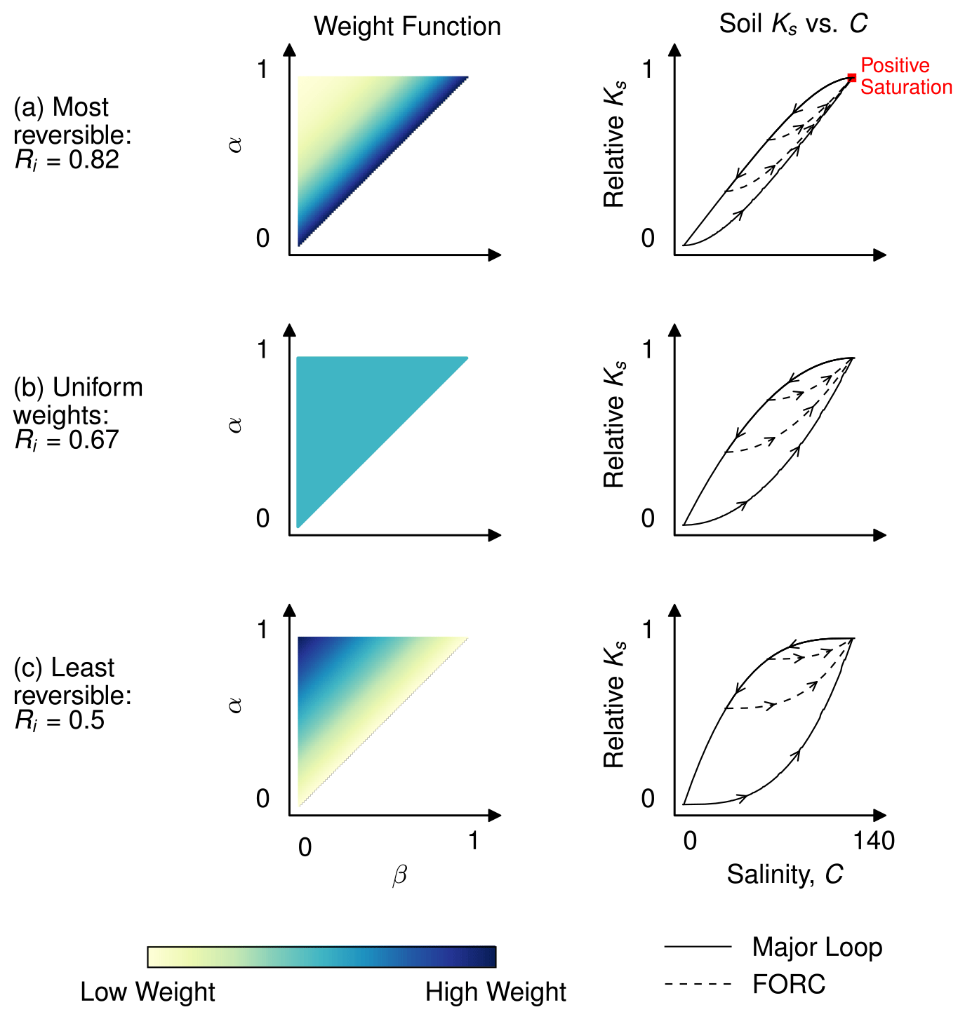
Figure 3 The degree to which a given soil is reversible and the shape of its hysteresis curves is determined by the soil's weight function (left column). Weight functions can be determined experimentally through the measurement of first-order reversal curves, FORCs (the dashed lines shown in the right-hand column). R_i refers to the reversibility index, with a value of one indicating full reversibility and a value of zero corresponding to full irreversibility.

2.3 Reversibility index

To facilitate quantitative comparison of the degree to which different soils are reversible, we use the weight function to define a reversibility index, R_i. The full development of the reversibility index is contained in Sect. C, but the fundamental idea behind it is that the closer the weight distribution is to the diagonal of the limiting triangle (i.e., the line α=β), the more reversible the soil, as in Fig. 3a. Conversely, as the weight distribution becomes closer to the vertex of the triangle in the top left (α_max, 0), the more irreversible the soil, as in Fig. 3c. The reversibility index is defined to range from 0 to 1, with a value of one indicating a completely reversible soil (no hysteresis) and a value of zero corresponding to a completely irreversible soil.

3 Determination of the weight function

As a result of the one-to-one correspondence between the weight function and the hysteresis graph, a soil's weight function can be determined by measuring its FORCs. In this section, we outline the experimental framework needed to measure FORCs and demonstrate how the data collected from these experiments can be used to determine a soil's weight function. While the experimental work necessary to compute weight functions for multiple soils is outside the scope of this paper, in what follows we present a “proof of concept” wherein we show limited FORC measurements and use these to construct a partial weight function. This proof of concept relies on soil column experiments, but we also note that the same framework could be used to measure FORCs in the field.

3.1 Experimental setup

Experiments to measure FORCs should begin with the same setup commonly used to study degradation of K_s due to salinity and sodicity (McNeal and Coleman, 1966; Ezlit et al., 2013; De Menezes et al., 2014). In these experiments, a fixed water head (H) is imposed on the soil column, so that K_s can be found using Darcy's law, $q=-K_{\mathrm{s}}\mathrm{\nabla }H$, where q is the discharge flux, and ∇H is the hydraulic head gradient. The SAR of the input water is typically held constant, as salinity is gradually reduced, with the procedure repeated for a range of SAR values. Conversely, the role of the variables can be flipped, with C held constant and the SAR of the applied water gradually increased. In either case, changes in K_s are recorded as the quality of the input water is changed. In the context of the Preisach framework, these experiments begin from “positive saturation”, i.e., the state when all hysterons are on. This corresponds to the point where both K_s and the input variable are maximal, as seen in the annotation in Fig. 3a. As the quality of the applied water is changed (C decreased or SAR increased), the experiments effectively sample the upper curve of the major hysteresis loop.

Measurement of FORCs can be achieved by extending the procedure described above so that, following the initial decline in K_s, we “reverse” the trend in water quality (now either towards higher C or lower SAR) and measure the response of K_s to conditions that favor improvements in soil structure. Several FORCs can be measured by repeating this procedure and varying the reversal point. For example, for the case when SAR is fixed, one should alter the point of minimum salinity at which the trend in C is reversed. In Fig. 3, two FORCs (the dashed lines) are shown for each hysteresis graph. Because the presented model considers changes in K_s as a result of both C and SAR, calculation of a particular soil's complete weight function requires the measurement of two sets of FORCs, one in which changes in K_s are measured as SAR is held constant, and one in which C is held constant.

After measuring several FORCs, the weight function can be calculated by taking the mixed partial derivative of the output (i.e., K_s) at points along these curves (Mayergoyz, 2003, see Eq. A4). An annotated example of the code necessary to compute the weight function from experimental data is included at https://github.com/yairmau/hysteresis-python (last access: 8 April 2021). We note that in the case where SAR is varied while C is kept constant, positive saturation occurs for low input values and not high values, as assumed in the presented graphs. In order to keep the mathematical framework the same for all cases, we define the two inputs in the code as C and −SAR, thus maintaining uniformity; K_s declines as the inputs are decreased.

3.2 Initial results

To showcase how FORCs can be used to calculate a soil's weight function, we conducted a limited experiment to measure FORCs on a test soil. In doing this, our goal is to demonstrate both the feasibility of such experiments and the suitability of the tools we developed to analyze the results. As such, this experiment does not constitute the whole set of procedures delineated above, which are necessary for the full characterization of a soil, but must be seen as a proof of concept. To the best of our knowledge, the results shown in this subsection are the first experimental account of the partial reversibility in K_s as influenced by salinity and sodicity.

In this experiment, we used a brown steppe soil (Ravikovitch, 1992), from the Kiryat Gat region of Israel, with 25 % clay content. We held SAR equal to 20 (mmol_c L⁻¹)${}^{-\mathrm{1}/\mathrm{2}}$ constant and measured K_s, as the value of C was repeatedly decreased and then increased. Measurements of K_s were recorded following the equilibration of the flow, the electrical conductivity, and the sodium concentration between the soil column's inflow and outflow solutions (in three replicates). The typical time for equilibration of a single measurement point was 3 h, after which determination of K_s was conducted, and the solution was changed for the next step of the procedure. For more details on the soil properties and experimental setup, see Sect. B.

Figure 4a shows the major loop of degradation and first-order reversal curves, starting from concentrations 5, 10, 15, 20, and 50 mmol_c L⁻¹. In what follows, we will refer to each FORC by its lowest concentration value. The degradation in K_s experienced by the soil before salinity was decreased below C equal to 20 mmol_c L⁻¹ was found to be fully reversible, as FORCs 20 and 50 depict (they overlap with the major loop). FORCs 5, 10, and 15 show partial reversibility only, with K_s not returning to its original value, even for very concentrated solutions of 400 mmol_c L⁻¹ (not shown in the graph).

We used the data from the FORCs in Fig. 4a to determine a limited weight function, shown in Fig. 4b. This is a limited weight function because it contains information on one SAR value only. Because the decay in K_s, shown by the major loop curve, is most pronounced for low C values, most of the weight is concentrated on the left of the triangle. Furthermore, the moderate rehabilitation in K_s shown by the FORCs also takes place in low C values; therefore, we see a higher density on the bottom of the triangle. Note that the triangle's upper input bounds are 300 mmol_c L⁻¹, while the experiment's upper bound was 200 mmol_c L⁻¹. This expansion of the triangle is necessary because the reversal curves do not go back to full rehabilitation (relative K_s=1.0), and according to Preisach's framework, the system always reaches full saturation upon arrival at the upper input bound. The expansion of the triangle leaves some weight beyond the experimental bounds (see the dotted line in Fig. 4b), thus allowing for incomplete rehabilitation.

In order to make sure that the weight triangle contains the information of the hysteresis graph, we modeled the soil's response using this weight function. The modeled results, shown in Fig. 4c, are quite similar to the experimental data of Fig. 4a. It is worth noting that the modeled FORCs return to higher K_s values, i.e., there is a slight overestimation of rehabilitation, and several FORCs converge as C increases. This is due to the effort to build a high-resolution picture of the weight function from very few data points. It is possible to eliminate this issue by increasing the number of FORCs (as shown in Fig. B1). Of course, this comes at the cost of additional time and resources, and we believe that our results are quite satisfactory, given the high level of upscaling involved in the process. The algorithm devised to reconstitute the weight function from experimental data (see the GitHub repository) incorporates both the qualitative and quantitative behavior of the soil under salinity and sodicity changes.

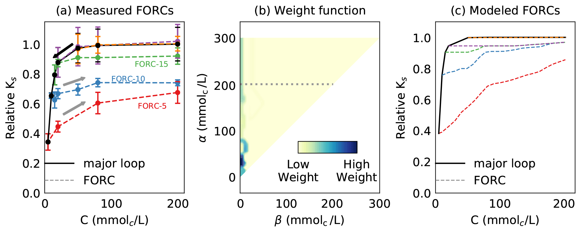
Figure 4 (a) Measured hysteresis in K_s, while keeping SAR equal to 20 (mmol_c L⁻¹)${}^{-\mathrm{1}/\mathrm{2}}$ constant. The major loop of degradation is shown by the solid black line, while FORCs are denoted by dashed lines. (b) The calculated weight function for the experimental data. Most of the weight is concentrated on the left side of the triangle as a light vertical strip and a heavy stain. (c) Modeled hysteresis graph using the weight function shown in panel (b). The accuracy of modeled results improves with the number of experimental points.

3.3 Insights for future experiments

This limited experiment yields a number of important insights, and we hope that these will prove useful to future efforts to characterize trends of partial reversibility in soil K_s.

The experimental setup is relatively simple, and the whole procedure is straightforward, although full characterization of a soil's weight function has the potential to be long and laborious. Determination of a soil's complete weight function requires measuring hysteresis graphs for at least five fixed SAR values (i.e., when C is varied, as seen in Fig. 4a) and for five fixed C values (i.e., when SAR is varied). Each of these hysteresis graphs must contain at least five FORCs, with each FORC itself requiring several measurement points. The suggested number of five is, of course, a rule of thumb. If one wishes to obtain weight functions of finer detail, then more hysteresis curves or FORCs per hysteresis could be measured. We do not recommend, however, measuring fewer than four hysteresis curves or fewer than four reversal curves, since this would translate into highly coarse weight functions, which would limit their usefulness.

Given the typical times of equilibration we experienced, we estimate that a full characterization of the soil hysteresis would take approximately 1 month. Soils with higher clay content may require significantly more time, since these soils can be expected to need additional time to equilibrate. Conversely, characterization of soils with a lower clay content may require less time than we have estimated here.

The first thing one should do before measuring the FORCs is to measure the major loop (i.e., the pattern of decay) to determine the range of input values in which K_s varies the most. The points of return of each FORC should be distributed roughly equally along the decay in K_s. For instance, Fig. 4a shows that the return points are more concentrated between concentrations 5 and 20 mmol_c L⁻¹ because these return points roughly sample the steepest decline in K_s. Conversely, return points where the slope of the major loop is flat do not yield as much useful information for characterizing the weight function. It is important to note that the measurement points along all FORCs have the same input values. This is necessary because of the way we developed our algorithm for building the weight functions.

4 Model applications

In this section, we use the model to demonstrate how consideration of hysteresis is essential when analyzing degradation and rehabilitation in soils. While controlled soil column experiments are expected to behave differently than field conditions, they still provide invaluable information regarding degradation and rehabilitation trends. More importantly, these experiments allow us to generate testable hypotheses on the interactions between soil and environmental conditions over the long run. However, the modeling formalism presented here is general and does not depend on the idiosyncrasies of particular experiments. This is to say that, while we measure FORCs using soil columns, FORCs could also be measured with field experiments. The lab experiments described here are a first attempt to parametrize and constrain the model, and further lab and field experiments are necessary to ensure the model's applicability in real-life conditions. At this stage, no experimental work has addressed the K_s hysteresis in detail. We incorporate results from the well-known McNeal and Coleman (1966) experiments to show how it is possible for soils with the same degradation patterns to exhibit very different levels of reversibility.

The experimental setup employed by McNeal and Coleman (1966) is ideal for this purpose because it resembles the degradation portion of the experimental procedure described in Sect. 3. Specifically, McNeal and Coleman (1966) measured K_s as input water of fixed SAR, but declining salinity, was applied to soil columns. The procedure was repeated for several SAR values, as shown in Fig. 5a, which reproduces the degradation curves presented by McNeal and Coleman (1966) for SAR 15, 25, 50, and 100 mmol${}_{\mathrm{c}}^{\mathrm{1}/\mathrm{2}}$ L${}^{-\mathrm{1}/\mathrm{2}}$ (henceforth, we will omit the units of SAR).

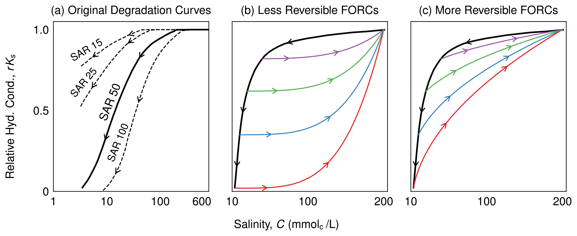
Figure 5 Different levels of irreversibility can be possible from the same degradation curve. (a) Degradation curves from experiments performed by McNeal and Coleman (1966). Note: results are presented on the logarithmic scale. The degradation curve associated with SAR 50 is used to construct two sets of possible FORCs, with one showing a low level of reversibility (b) and the other a high level of reversibility (c).

The possibility for different levels of reversibility, given the same degradation curves, is presented in Fig. 5b and c. Here, we use the degradation curve associated with SAR 50 to construct two potential sets of FORCs. The FORCs in Fig. 5b correspond to a low level of reversibility – once the soil has been degraded, an increase to higher K_s values requires a significant increase in salinity. By contrast, the FORCs in Fig. 5c indicate a high level of reversibility, such that K_s values are more easily restored following degradation. It is important to emphasize that we constructed both sets of presented FORCs, and that neither derive from experiments. That is, they are meant to demonstrate the need for detailed experiments on irreversibility, according to the guidelines discussed in Sect. 3, which will allow us to more accurately determine the true extent to which a given soil exhibits hysteresis in degradation and rehabilitation. We also note that even the concave FORCs in Fig. 5c consider a higher level of irreversibility than existing models for degradation and rehabilitation, which allow K_s to increase by returning along the original degradation curve (i.e., the top curve of the major loop).

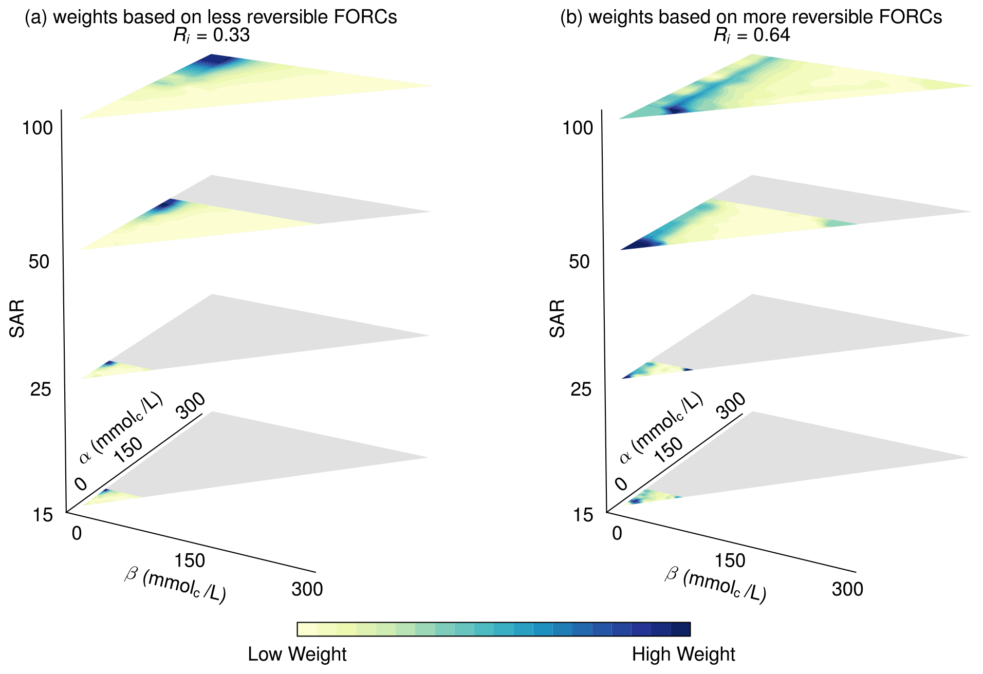
Figure 6 Potential weight functions, showing low (a) and high (b) levels of reversibility, are constructed based on the degradation experiments in McNeal and Coleman (1966). (a) Weight functions based on less reversible FORCs; reversibility index is R_i=0.33. (b) Weight functions based on more reversible FORCs; reversibility index is R_i=0.64.

By extending the approach used in Fig. 5b and c, we produce two potential weight functions based on the degradation curves in McNeal and Coleman (1966). To do this, we first construct two sets of FORCs (low and high reversibility) for each of the respective SAR values (15, 25, 50, and 100). We then use these FORCs to compute weight functions, using the technique and code described in Sect. 3. The resulting weight functions are presented in Fig. 6. The different areas occupied by the limiting triangle in these plots reflect the different values of C_max – the unique salinity value at which degradation begins – for each respective SAR value. When determining the weight function, salinity values greater than u_max are not assigned any weights.

Examination of the weight functions in Fig. 6 shows the crucial way in which our model is able to distinguish between less reversible and more reversible soils. Focusing first on SAR 100, we observe that, for the weight function derived from the less reversible FORCs (Fig. 6a), the heavy weights are concentrated exclusively in the region close to (α_max, 0). For the weight function derived from the more reversible FORCs (Fig. 6b), the heavy weights are similarly concentrated in the region for which β is close to zero. A major contrast can be seen, however, in the distribution of the weights along the α axis, with the heavy weights in the more reversible case distributed along the entire α axis and not only in the region for which α is large, as is the case for the less reversible example. In both examples, the weight distributions along the β axis are identical because this axis is associated with degradation, and both weight functions were derived from the same degradation data. The concentration of weights in the region where β is low reflects the soil's relative resilience to degradation when salinity is high, as seen in Fig. 5. The α axis, by contrast, is associated with rehabilitation. Because the weights in Fig. 6b are distributed along the entire α axis, we can expect any increase in salinity to lead to an increase in K_s, matching the pattern observed in the FORCs from which the weight function was derived. In Fig. 6a, on the other hand, the heavy weights are concentrated in the region for which α is high, such that increases in K_s will only occur when salinity crosses some specific threshold, again reflecting what we expect based on the FORCs. Similar patterns are observed for SAR 50, 25, and 15.

The difference between these two weight functions can be expressed quantitatively by calculating the reversibility index for each. For the weights in Fig. 6a, the reversibility index is R_i=0.33, while for the weights in Fig. 6b the reversibility index is R_i=0.64. In this case, we are comparing two sets of hypothesized FORCs based on the same soil, but we believe the reversibility index's true power is in its ability to compare between different soil types. The index gives us a tool to speak precisely about the degree of reversibility, without having to resort to vague descriptions of soils being “more” or “less” reversible.

It is worth mentioning that the weight “stacks” of Fig. 6 are only half the complete weight function. Their complement is another set of stacks, where the vertical axis is salinity concentration, C, while α and β refer to SAR. For simplicity's sake, these extra stacks are not shown here, but an example can be seen in Fig. C1 of Sect. C.

While the discussion up to now has not considered dynamics, integration of the presented framework with models for salinity and sodicity dynamics would allow us to consider the influence of a soil's previous degradation and rehabilitation cycles on its future state. This is a crucial step in improving our ability to assess the risk of soil degradation because often degradation is triggered by seasonal patterns, which may only lead to significant declines in K_s after a number of years. While models that consider changes in K_s to be reversible are unable to capture the sort of cumulative damage that may result from such cycles, our model is ideally suited for this purpose because it makes future values of K_s dependent on the soil's history. As seen here, we can expect that the soil's weight function will play a crucial role in determining the risk of irreversible soil degradation past critical thresholds. These insights, however, can only be obtained if we widen our attention from traditional degradation experiments and begin to focus on rehabilitation processes through FORC measurements, as demonstrated here.

5 Discussion and conclusions

The model developed here is the first to consider irreversibility in soil degradation as a result of water quality. Specifically focused on changes to K_s as a result of salinity and sodicity, the model demonstrates how hysteresis has the potential to significantly affect our expectations of soil rehabilitation following declines in K_s. The model accounts for soil-specific differences, using a weight function, which allows us to ascertain a given soil's future response to any change in water quality. In this paper, we demonstrated how a soil's weight function can be determined from experimental data, namely the measurement of first-order reversal curves or FORCs. We showcased how to parameterize the model with FORCs obtained from soil column experiments, but in the future, field experiments could increase our understanding of rehabilitation mechanisms in a richer and more realistic environment over longer timescales. Much more than the major loop curves, the FORCs are key to the full characterization of a soil's irreversible behavior. To the best of our knowledge, the scant experimental literature on irreversible decay in K_s (Dane and Klute, 1977) did not exhibit any measurements of FORCs. The experimental results presented here, therefore, are the first to measure FORCs and underscore the need to focus on these measurements, serving as a typical example of the beneficial interaction between theory and experiments.

As a measure of the degree to which a given soil can be rehabilitated following degradation, we introduced a reversibility index. The reversibility index uses the soil's weight functions to quantify the degree to which a given soil is reversible. With this index, one can directly compare the degree to which different soils are susceptible to irreversible degradation. This represents an important advance beyond qualitative statements (e.g., the soil with the greater clay content is more prone to irreversible degradation).

The reversibility index is a convenient quantitative measure; however, it does not determine the risk of irreversible degradation given a particular climate and irrigation regime (Kramer and Mau, 2020). This risk depends on the specific history a soil has been through, and further research is required to unravel the interplay between soil characteristics, environmental drivers, and the actual dynamics of water and solutes in the soil. To this end, a critical next step will be the integration of the model presented here with leading numerical models used for studying the dynamics of soil salinity and sodicity over the long term. At present, all such models consider changes in K_s to be completely reversible (R_i=1), limiting our ability to predict and control the fate of agricultural soils in the face of global climatic change and dwindling water resources.

Finally, while this work focused on the effects of salinity and sodicity on K_s, we believe the conceptual foundation offered by the Preisach framework may have wide-ranging application to other soil processes. As demonstrated here, and in its application to modeling hysteresis in soil moisture patterns (Flynn et al., 2006; McNamara, 2014), a major appeal of the Preisach framework is its generality and lack of major assumptions. This stands in contrast to other models that have been used to describe hysteresis phenomena in soil science, such as those that focus on the response of water retention curves to drying and wetting (Mualem, 1974; Parlange, 1976; Haverkamp et al., 2002). Parlange's 1976 model, for instance, assumes that all hysteresis curves have the same shape (e.g., following van Genuchten's equation). As we argue here, at this point, our understanding on the degree of reversibility in K_s is still based on extremely limited experimental data, and we find no justification for the significant assumption that all reversal curves should have shape similarity with the major hysteresis loop curves. We believe that the Preisach approach is advantageously suited to studying hysteresis in K_s, specifically because of its ability to consider various secondary factors, including soil texture and mineralogy.

Beyond salinity and sodicity, the framework may be adapted to address research questions related to covariates, including composition, clay mineralogy, and soil pH among others. We do note that, while the mathematical formalism admits any number of inputs, that does not mean that the optimal way to use the presented framework would be to increase the number of input variables. We believe that using more than two inputs would obfuscate the understanding of the hysteresis process. Each additional input variable would require a corresponding weight function, such that more than two input variables would require an impractical number of experiments for determining the weights. Nonetheless, we believe that the framework presented here may be of great use to studying the aforementioned soil processes in their own right, especially because many of them are marked by hysteresis. To that end, we encourage readers to make use of our code, all of which is accessible in the repository for this paper.

Appendix A: The Preisach framework

For the case of a single input variable, we can use the Preisach framework to determine the output value, f(t), for a given input, u(t), by integrating over the limiting triangle such that, in the following:

$$\begin{array}{}\text{(A1)}& f\left(t\right)=\underset{\mathit{\alpha }\ge \mathit{\beta }}{\iint }\mathit{\mu }(\mathit{\alpha },\mathit{\beta }){\widehat{\mathit{\gamma }}}_{\mathit{\alpha }\mathit{\beta }}u\left(t\right)\mathrm{d}\mathit{\alpha }\mathrm{d}\mathit{\beta },\end{array}$$

where $\widehat{\mathit{\gamma }}$ is an operator that indicates the state of the hysteron, i.e., whether it is on or off given the value of u(t), and μ(α,β) is the weight function (Mayergoyz, 2003).

The weight function, μ(α,β), can be determined experimentally, as described in Sect. 3, by measuring output along the FORCs. Specifically, the experimental procedure calls for starting at positive saturation (u=u_max) and then reducing input so that $u={\mathit{\beta }}^{\prime }$. The output on the FORCs then corresponds to the values as input is gradually increased from β^′ to $u={\mathit{\alpha }}^{\prime }$, as shown in Fig. A1. The output at points (α^′, β^′) is denoted $f_{{\mathit{\alpha }}^{\prime }{\mathit{\beta }}^{\prime }}$. The weight at a given point (α^′, β^′) on the FORC can be found according to the following equation (Mayergoyz, 2003):

$$\begin{array}{}\text{(A2)}& \mathit{\mu }({\mathit{\alpha }}^{\prime },{\mathit{\beta }}^{\prime })={\displaystyle \frac{\mathrm{1}}{\mathrm{2}}}{\displaystyle \frac{{\partial }^{\mathrm{2}}{f}_{{\mathit{\alpha }}^{\prime }{\mathit{\beta }}^{\prime }}}{\partial {\mathit{\alpha }}^{\prime }\partial {\mathit{\beta }}^{\prime }}}.\end{array}$$

For the case when there are two inputs, u(t) and v(t), then Eq. (A1) is expanded so that, in the following:

$$\begin{array}{}\text{(A3)}& \begin{array}{rl}f\left(t\right)& =\underset{\mathit{\alpha }\ge \mathit{\beta }}{\iint }\mathit{\mu }(\mathit{\alpha },\mathit{\beta },v(t\left)\right){\widehat{\mathit{\gamma }}}_{\mathit{\alpha }\mathit{\beta }}u\left(t\right)\mathrm{d}\mathit{\alpha }\mathrm{d}\mathit{\beta }\\ & +\underset{\mathit{\alpha }\ge \mathit{\beta }}{\iint }\mathit{\nu }(\mathit{\alpha },\mathit{\beta },u(t\left)\right){\widehat{\mathit{\gamma }}}_{\mathit{\alpha }\mathit{\beta }}v\left(t\right)\mathrm{d}\mathit{\alpha }\mathrm{d}\mathit{\beta },\end{array}\end{array}$$

where μ and ν are the respective weight functions (Mayergoyz, 2003). The dependency of μ and ν on v and u, respectively, serves to couple the inputs. The weight functions μ and ν are given by the following (Mayergoyz, 2003):

$$\begin{array}{}\text{(A4a)}& {\displaystyle }& {\displaystyle }\mathit{\mu }(\mathit{\alpha },\mathit{\beta },v)={\displaystyle \frac{{\partial }^{\mathrm{2}}F(\mathit{\alpha },\mathit{\beta },v)}{\partial \mathit{\alpha }\partial \mathit{\beta }}}\text{(A4b)}& {\displaystyle }& {\displaystyle }\mathit{\nu }(\mathit{\alpha },\mathit{\beta },u)={\displaystyle \frac{{\partial }^{\mathrm{2}}G(\mathit{\alpha },\mathit{\beta },u)}{\partial \mathit{\alpha }\partial \mathit{\beta }}},\end{array}$$

where F and G are defined as follows (Mayergoyz, 2003):

$$\begin{array}{}\text{(A5a)}& {\displaystyle }& {\displaystyle }F(\mathit{\alpha },\mathit{\beta },v)={\displaystyle \frac{\mathrm{1}}{\mathrm{2}}}\left(f_{\mathit{\alpha }\mathit{\beta }v}-f_{\mathit{\beta }v}^{+}\right)\text{(A5b)}& {\displaystyle }& {\displaystyle }G(\mathit{\alpha },\mathit{\beta },u)={\displaystyle \frac{\mathrm{1}}{\mathrm{2}}}\left(f_{u\mathit{\alpha }\mathit{\beta }}-f_{u\mathit{\beta }}^{+}\right).\end{array}$$

Here, $f_{\mathit{\beta }v}^{+}$ denotes the “branching” point of the FORC output for a fixed value of v(t). Likewise, f_αβv corresponds to the output as we move along the FORC by increasing the value of α, following the same methodology as in the one input case.

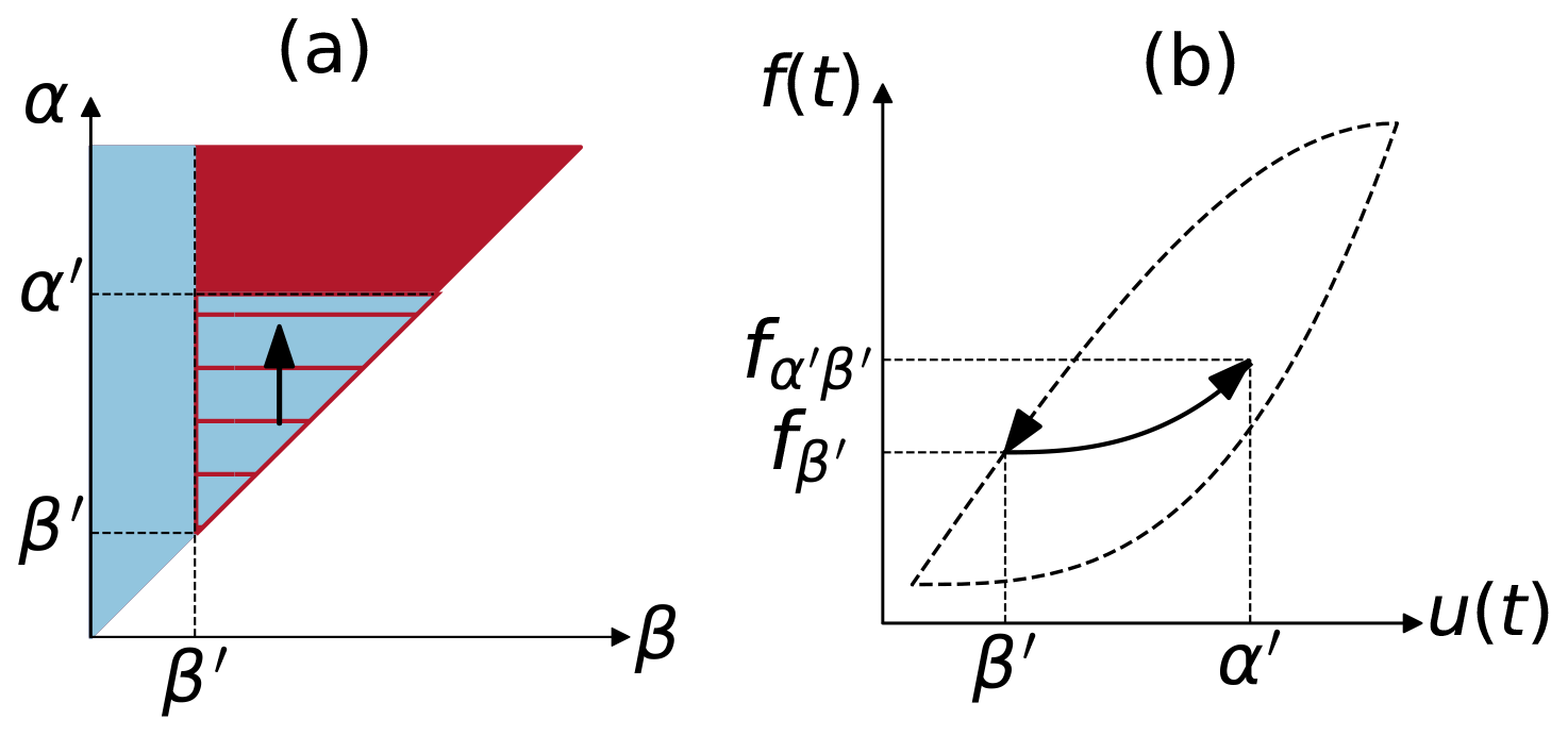
Figure A1 Output along the FORC is used to find the weight function, μ(α,β). For the case with a single input variable, the weight of the hysteron at (α^′, β^′) can be found by starting at positive saturation (u=u_max), decreasing input to $u={\mathit{\beta }}^{\prime }$, and then gradually increasing input to $u={\mathit{\alpha }}^{\prime }$. Changes in the fraction of the hysterons in the limiting triangle that are on (a) result in changes in output (b).

Appendix B: Experimental setup

We measured saturated hydraulic conductivity, K_s, in soil columns (length – 5.0 cm; internal diameter – 5.4 cm) within transparent perspex pipes (length – 8.0 cm; external diameter – 6.0 cm), where the hydraulic head H=31 cm was maintained constant using a Mariotte's bottle. The air-dried soil was sieved through a 2 mm sieve and packed to a bulk density of 1.30 g cm⁻³. For each column, a soil mass of 149 g, divided into five equal parts, was packed into the pipe and bulked with equal pressure to ensure uniform packing across the length of the columns and between all 15 columns. The soil was lined with a geotex fiber, and the pipes were closed at both ends with rubber stoppers. The soil columns were allowed to capillary wet with a solution of concentration 200 mmol_c L⁻¹ and SAR equal to 20 (mmol_c L⁻¹)${}^{-\mathrm{1}/\mathrm{2}}$ for at least 4 h. Upon saturation, leaching started from the top of the soil column. While SAR equal to 20 (mmol_c L⁻¹)${}^{-\mathrm{1}/\mathrm{2}}$ was kept constant, solutions of decreasing concentrations were made to flow through the columns (200, 80, 50, 20, 15, 10, and 5 mmol_c L⁻¹). For each concentration, K_s was measured using Darcy's equation only upon equilibration of the efflux with respect to flow rate, electrical conductivity, and sodium concentration. Electrical conductivity and sodium concentration were measured with a Mettler Toledo InLab 752-6mm and perfectION comb NA, respectively. A total of three replicates were used for each K_s measurement.

The soil used in the experiment is a brown steppe soil (Ravikovitch, 1992) from the Kiryat Gat region of Israel. The measured soil texture is 25 % clay, 25 % silt, and 50 % sand (PARIO soil particle size analyzer; METER Group, Inc.). The dominant clay mineral is montmorillonite (60 %), and the soil's CaCO₃ content is 16 %.

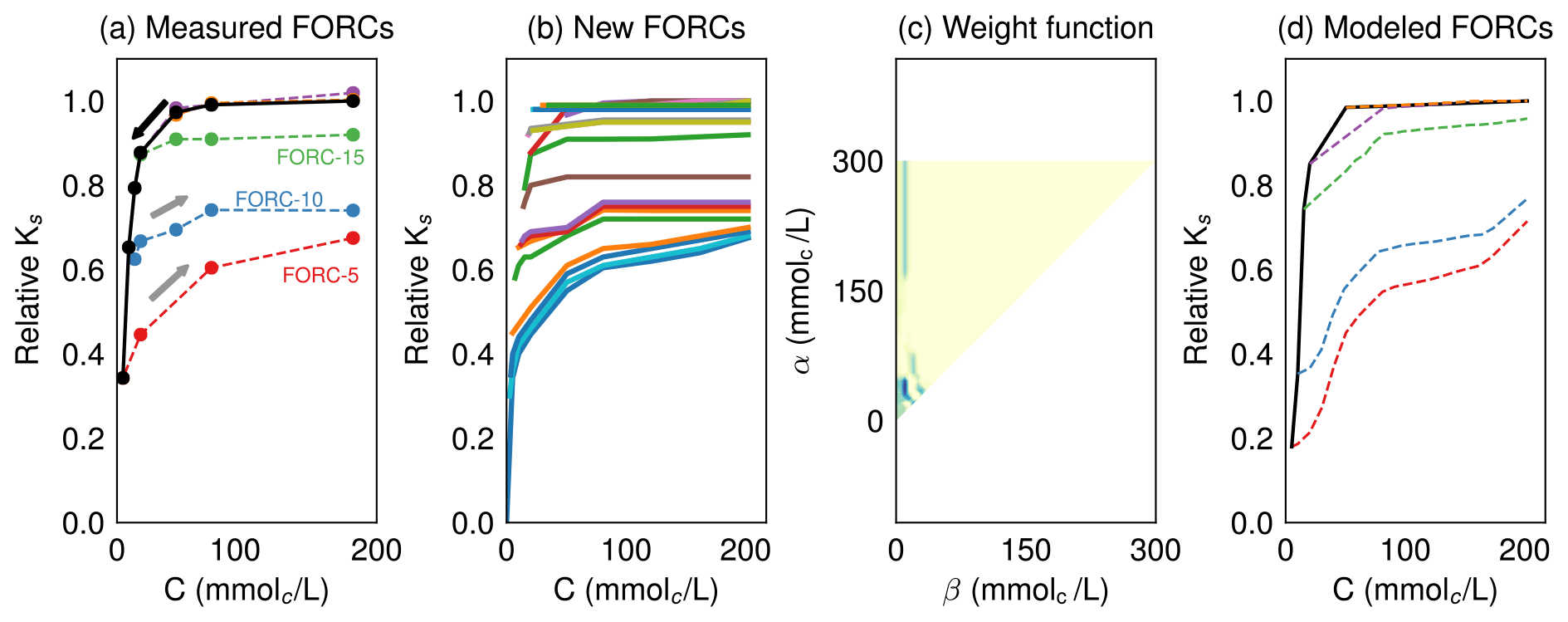
Figure B1 Experimental results (a) can be augmented by interpolated FORCs (b), resulting in a finer weight function (c), which, in turn, can reproduce the initial data more faithfully (d). This exercise demonstrates that increasing the number of experimental points will yield more accurate predictions, exemplifying the well-known tradeoff between resource expenditures (more data) and accuracy.

Appendix C: Reversibility index

It is easiest to start defining the reversibility index R_i for the case of a single input variable as follows:

$$\begin{array}{}\text{(C1)}& R_i=\mathrm{1}-{\displaystyle \frac{\sqrt{\mathrm{2}}}{u_{\max }}}{\displaystyle \frac{I\left[\mathit{\mu }\right(\mathit{\alpha },\mathit{\beta }\left)\mathcal{D}\right(\mathit{\alpha },\mathit{\beta }\left)\right]}{I\left[\mathit{\mu }\right(\mathit{\alpha },\mathit{\beta }\left)\right]}},\end{array}$$

where I denotes the integral over the limiting triangle as follows:

$$\begin{array}{}\text{(C2)}& I\left[f\right(\mathit{\alpha },\mathit{\beta }\left)\right]=\underset{\mathrm{0}}{\overset{u_{\max }}{\int }}\mathrm{d}\mathit{\alpha }\underset{\mathrm{0}}{\overset{\mathit{\alpha }}{\int }}\mathrm{d}\mathit{\beta }f(\mathit{\alpha },\mathit{\beta }),\end{array}$$

and, in the following:

$$\begin{array}{}\text{(C3)}& \mathcal{D}(\mathit{\alpha },\mathit{\beta })={\displaystyle \frac{\mathit{\alpha }-\mathit{\beta }}{\sqrt{\mathrm{2}}}}\end{array}$$

is the Euclidean distance of a point (α, β) in the limiting triangle to the diagonal α=β. The reversibility index is $\mathrm{0}\le R_i\le \mathrm{1}$, where R_i=1 means total reversibility, and R_i=0 means total irreversibility. In this definition, we assume that the input varies between $\mathrm{0}\le u\le u_{\max }$. In the more general case that the input u varies between $u_{\min }\le u\le u_{\max }$, then the denominator in Eq. (C1) should be substituted by u_max−u_min and the integration limits in Eq. (C2) accordingly.

The intuition behind this definition is as follows. Every point (α, β) in the weight function μ is itself weighted by its distance to the diagonal α=β, given by the function 𝒟(α,β). If all the weights in μ are concentrated along this diagonal, then we have that 𝒟=0, and the reversibility index yields 1, meaning complete reversibility. On the other extreme, if all the weight in μ is as far as possible from the diagonal, namely concentrated at the point (α=u_max, β=0), then the reversibility index yields 0, i.e., total irreversibility. The denominator I[μ(α,β)] in Eq. (C1) simply normalizes the weight function to 1, while the factor $\frac{\sqrt{\mathrm{2}}}{u_{\max }}$ normalizes the maximal distance to 1. Roughly speaking, the more weight is concentrated near the diagonal α=β, the thinner the major hysteresis loop and the higher the reversibility index, R_i. Conversely, the further the weight is from the diagonal, the wider the major hysteresis loop, and consequently, R_i will be closer to zero. Of course, the factor $\sqrt{\mathrm{2}}$ in Eq. (C1) could be canceled out with the same factor in the distance function 𝒟. We chose to leave 𝒟 as defined to maintain the link between the reversibility index and the distance of the weights from the diagonal α=β.

We can now expand the definition of R_i for two input variables as follows:

$$\begin{array}{}\text{(C4)}& \begin{array}{rl}{R}_i& =\mathrm{1}-{\displaystyle \frac{\mathrm{1}}{\mathrm{2}}}\left[{\displaystyle \frac{\sqrt{\mathrm{2}}}{u_{\max }}}{\displaystyle \frac{I\left[\mathit{\mu }\right(\mathit{\alpha },\mathit{\beta },v\left(t\right)\left)\mathcal{D}\right(\mathit{\alpha },\mathit{\beta }\left)\right]}{I\left[\mathit{\mu }\right(\mathit{\alpha },\mathit{\beta },v\left(t\right)\left)\right]}}\right.\\ & \left.+{\displaystyle \frac{\sqrt{\mathrm{2}}}{v_{\max }}}{\displaystyle \frac{I\left[\mathit{\nu }\right(\mathit{\alpha },\mathit{\beta },u\left(t\right)\left)\mathcal{D}\right(\mathit{\alpha },\mathit{\beta }\left)\right]}{I\left[\mathit{\nu }\right(\mathit{\alpha },\mathit{\beta },u\left(t\right)\left)\right]}}\right],\end{array}\end{array}$$

where now I denotes the following:

$$\begin{array}{}\text{(C5)}& I\left[f\right(\mathit{\alpha },\mathit{\beta },w\left)\right]=\underset{\mathrm{0}}{\overset{u_{\max }}{\int }}\mathrm{d}\mathit{\alpha }\underset{\mathrm{0}}{\overset{\mathit{\alpha }}{\int }}\mathrm{d}\mathit{\beta }\underset{\mathrm{0}}{\overset{w_{\max }}{\int }}\mathrm{d}wf(\mathit{\alpha },\mathit{\beta },w).\end{array}$$

The brackets in Eq. (C4) simply show the arithmetic mean of the same operation done in Eq. (C1), computed for the weight densities μ and ν.

C1 Discrete version of R_i

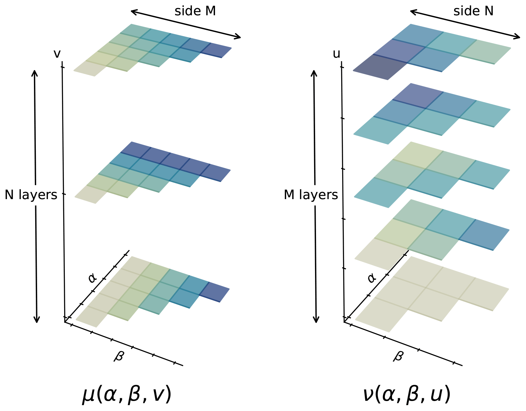
Often the weight functions μ and ν will be calculated numerically from experimental data, as done in Sect. 4 (see also our full code and widget on GitHub). In this case, μ (ν) will be composed of N (M) discrete stacked layers, each composed by right triangles of side M (N) (see Fig. C1). The reversibility index in the discrete case then becomes the following:

$$\begin{array}{}\text{(C6)}& \begin{array}{rl}{R}_i& =\mathrm{1}-{\displaystyle \frac{\mathrm{1}}{\mathrm{2}}}\left[{\displaystyle \frac{\sqrt{\mathrm{2}}}{M}}{\displaystyle \frac{\sum _k^N\sum _{i\ge j}^M\mathit{\mu }(i,j,k)\mathcal{D}(i,j)}{\sum _k^N\sum _{i\ge j}^M\mathit{\mu }(i,j,k)}}\right.\\ & \left.+{\displaystyle \frac{\sqrt{\mathrm{2}}}{N}}{\displaystyle \frac{\sum _k^M\sum _{i\ge j}^N\mathit{\nu }(i,j,k)\mathcal{D}(i,j)}{\sum _k^M{\sum }_{i\ge j}^N\mathit{\nu }(i,j,k)}}\right],\end{array}\end{array}$$

and for the particular case of one input only, it reads as follows:

$$\begin{array}{}\text{(C7)}& R_i=\mathrm{1}-{\displaystyle \frac{\sqrt{\mathrm{2}}}{N}}{\displaystyle \frac{\sum _{i\ge j}^N\mathit{\mu }(i,j)\mathcal{D}(i,j)}{\sum _{i\ge j}^N\mathit{\mu }(i,j)}}.\end{array}$$

Note that $\sum _{i\ge j}^N$ represents the double summation $\sum _i^N\sum _j^i$. Figure C1 depicts an example of the discrete weight functions for N=3 and M=5.

C2 Some simple cases

We calculate here the one input reversibility index of three simple examples in order to build some intuition of how R_i relates to specific weight distributions.

C2.1 Uniform weight distribution

For uniform $\mathit{\mu }(\mathit{\alpha },\mathit{\beta })=c_{\mathrm{0}}$, the reversibility index reads as follows:

$$\begin{array}{}\text{(C8)}& R_i={\displaystyle \frac{\mathrm{2}}{\mathrm{3}}}.\end{array}$$

C2.2 Thin diagonal weight distribution

The weight distribution $\mathit{\mu }(\mathit{\alpha },\mathit{\beta })=\mathit{\delta }(\mathit{\alpha }-\mathit{\beta }-c_{\mathrm{0}}{u}_{\max })$, where $\mathrm{0}\le c_{\mathrm{0}}\le \mathrm{1}$ corresponds to an infinitesimally thin diagonal line in the (α, β) plane (δ is the Dirac delta). This diagonal line can be offset from the origin by c₀u_max. Its reversibility index reads as follows:

$$\begin{array}{}\text{(C9)}& R_i=\mathrm{1}-c_{\mathrm{0}}.\end{array}$$

For c₀=0 there is no offset, and the diagonal line sits at α=β; therefore, R_i=1. As the offset is increased, R_i decreases until R_i=0 for c₀=1.

C2.3 Dirac delta weight distribution

In the case that all the weight distribution is concentrated at a single point ($\mathit{\alpha }=a_{\mathrm{0}}{u}_{\max },\mathit{\beta }=b_{\mathrm{0}}{u}_{\max }$), the distribution reads $\mathit{\mu }(\mathit{\alpha },\mathit{\beta })=\mathit{\delta }(\mathit{\alpha }-a_{\mathrm{0}}{u}_{\max })\mathit{\delta }(\mathit{\beta }-b_{\mathrm{0}}{u}_{\max })$, where a₀, $b_{\mathrm{0}}\in [\mathrm{0},\mathrm{1}]$. The reversibility index then yields the following:

$$\begin{array}{}\text{(C10)}& R_i=\mathrm{1}-\left(a_{\mathrm{0}}-b_{\mathrm{0}}\right).\end{array}$$

Again, when the weight distribution is on the diagonal line of the limiting triangle (a₀=b₀), we have R_i=1. As the locus of the distribution moves away from this diagonal, the reversibility index decreases.

Figure C1 The discrete representation of the weight functions $\mathit{\mu }(\mathit{\alpha },\mathit{\beta },v)$ and $\mathit{\nu }(\mathit{\alpha },\mathit{\beta },u)$.