Assessing the value of seasonal hydrological forecasts for improving water resource management: insights from a pilot application in the UK

Improved skill of long-range weather forecasts has motivated an increasing effort towards developing seasonal hydrological forecasting systems across Europe. Among other purposes, such forecasting systems are expected to support better water management decisions. In this paper we evaluate the potential use of a real-time optimization system (RTOS) informed by seasonal forecasts in a water supply system in the UK. For this purpose, we simulate the performances of the RTOS fed by ECMWF seasonal forecasting systems (SEAS5) over the past 10 years, and we compare them to a benchmark operation that mimics the common practices for reservoir operation in the UK. We also attempt to link the improvement of system performances, i.e. the forecast value, to the forecast skill (measured by the mean error and the continuous ranked probability skill score) as well as to the bias correction of the meteorological forcing, the decision maker priorities, the hydrological conditions and the forecast ensemble size. We find that in particular the decision maker priorities and the hydrological conditions exert a strong influence on the forecast skill–value relationship. For the (realistic) scenario where the decision maker prioritizes the water resource availability over energy cost reductions, we identify clear operational benefits from using seasonal forecasts, provided that forecast uncertainty is explicitly considered by optimizing against an ensemble of 25 equiprobable forecasts. These operational benefits are also observed when the ensemble size is reduced up to a certain limit. However, when comparing the use of ECMWF-SEAS5 products to ensemble streamflow prediction (ESP), which is more easily derived from historical weather data, we find that ESP remains a hard-to-beat reference, not only in terms of skill but also in terms of value.

1 Introduction

In a water-stressed world, where water demand and climate variability (IPCC, 2013) are increasing, it is essential to improve the efficiency of existing water infrastructure along with, or possibly in place of, developing new assets (Gleick, 2003). In the current information age there is a great opportunity to do this by improving the ways in which we use hydrological data and simulation models (the “information infrastructure”) to inform operational decisions (Gleick et al., 2013; Boucher et al., 2012).

Hydrometeorological forecasting systems are a prominent example of information infrastructure that could be used to improve the efficiency of water infrastructure operation. The usefulness of hydrological forecasts has been demonstrated in several applications, particularly to enhance reservoir operations for flood management (Voisin et al., 2011; Wang et al., 2012; Ficchì et al., 2016) and hydropower production (Faber and Stedinger, 2001; Maurer and Lettenmaier, 2004; Alemu et al., 2010; Fan et al., 2016). In these types of systems, we usually find a strong relationship between the forecast skill (i.e. the forecast ability to anticipate future hydrological conditions) and the forecast value (i.e. the improvement in system performance obtained by using forecasts to inform operational decisions). However, this relationship becomes weaker for water supply systems, in which the storage buffering effect of surface and groundwater reservoirs may reduce the importance of the forecast skill (Anghileri et al., 2016; Turner et al., 2017), particularly when the reservoir capacity is large (Maurer and Lettenmaier, 2004; Turner et al., 2017). Moreover, in water supply systems, decisions are made by considering the hydrological conditions over lead time of several weeks or even months. Forecast products with such lead times, i.e. “seasonal” forecasts, are typically less skilful compared to the short-range forecasts used for flood control or hydropower production applications.

When using seasonal hydrological scenarios or forecasts to assist water system operations, three main approaches are available: worst case scenario, ensemble streamflow prediction (ESP) and dynamical streamflow prediction (DSP). In the worst-case scenario approach, operational decisions are made by simulating their effects against a repeat of the worst hydrological droughts on records. Worst-case forecasts clearly have no particular skill, but their use has the advantage of providing a lower bound of system performance, and they reflect the risk-adverse attitude of most water management practice. This approach is commonly applied by water companies in the UK, and it is reflected in the water resource management planning guidelines of the UK Environment Agency (Environment Agency, 2017).

In the ensemble streamflow prediction (ESP) approach, a hydrological forecasts' ensemble is produced by forcing a hydrological model using the current initial hydrological conditions and historical weather data over the period of interest (Day, 1985). Operational decisions are then evaluated against the ensemble. The skill of the ESP ensemble is mainly due to the updating of the initial conditions. Since ESP forecasts are based on the range of past observations, they can have limited skill under non-stationary climate and where initial conditions do not dominate the seasonal hydrological response (Arnal et al., 2018). Nevertheless, the ESP approach is popular among operational agencies thanks to its simplicity, low cost, efficiency and its intuitively appealing nature (Bazile et al., 2017). Some previous studies assessed the potential of seasonal ESP to improve the operation of supply–hydropower systems. For example, Alemu et al. (2010) reported achieving an average economic benefit of 7 % with respect to the benchmark operation policy, whereas Anghileri et al. (2016) reported no significant improvements (possibly because they only used the ESP mean, instead of the full ensemble).

Last, the dynamical streamflow prediction (DSP) approach uses numerical weather forecasts produced by a dynamic climate model to feed the hydrological model (instead of historical weather data). The output is also an ensemble of hydrological forecasts, whose skill comes from both the updated initial condition and the predictive ability of the numerical weather forecasts. The latter is due to global climate teleconnections such as the El Niño–Southern Oscillation (ENSO) and the North Atlantic Oscillation (NAO). Therefore, DSP forecasts are generally more skilful in areas where climate teleconnections exert a strong influence, such as tropical areas, and particularly in the first month ahead (Block and Rajagopalan, 2007). In areas where climate teleconnections have a weaker influence, DSP can have lower skill than ESP, particularly beyond the first lead month (Arnal et al., 2018; Greuell et al., 2019). Nevertheless, recent advances in the prediction of climate teleconnections in Europe, such as the NAO (Wang et al., 2017; Scaife et al., 2014; Svensson et al., 2015), means that seasonal forecasts' skill is likely to continue increasing in the coming years. Post-processing techniques such as bias correction can also potentially improve seasonal streamflow forecast skill (Crochemore et al., 2016). Studies assessing the benefits of bias correction for seasonal hydrological forecasting are still rare in the literature. While bias correction is often recommended or even required for impact assessments to improve forecast skills (Zalachori et al., 2012; Schepen et al., 2014; Ratri et al., 2019; Jabbari and Bae, 2020), studies on long-term hydrological projections (Ehret et al., 2012; Hagemann et al., 2011) highlighted a lack of clarity on whether bias correction should be applied or not. In recent years, meteorological centres such as the European Centre for Medium-Range Weather Forecasts (ECMWF) and the UK Met Office have made important efforts to provide skilful seasonal forecasts, both meteorological (Hemri et al., 2014; MacLachlan et al., 2015) and hydrological (Bell et al., 2017; Arnal et al., 2018), in the UK and Europe and encouraged their application for water resource management. To the best of our knowledge, however, pilot applications demonstrating the value of such seasonal forecast products to improve operational decisions are mainly lacking and have only very recently started to appear (Giuliani et al., 2020).

While the skill of DSP is likely to keep increasing in the next years, it may still remain low at lead times relevant for the operation of water supply systems. Nevertheless, a number of studies have demonstrated that other factors, which are not necessarily captured by forecast skill scores, may also be important to improve the forecast value. These include accounting explicitly for the forecast uncertainty in the system operation optimization (Yao and Georgakakos, 2001; Boucher et al., 2012; Fan et al., 2016), using less rigid operation approaches (Yao and Georgakakos, 2001; Brown et al., 2015; Georgakakos and Graham, 2008) and making optimal operational decisions during severe droughts (Turner et al., 2017; Giuliani et al., 2020). Additionally, the forecast skill itself can be defined in different ways, and it is likely that different characteristics of forecast errors (sign, amount, timing, etc.) affect the forecast value in different ways. Widely used skill scores for hydrological forecast ensembles are the rank histogram (Anderson, 1996), the relative operating characteristic (Mason, 1982) and the ranked probability score (Epstein, 1969). The ranked probability score is widely used by meteorological agencies since it provides a measure of both the bias and the spread of the ensemble in a single factor, while it can also be decomposed into different sub-factors in order to look at the different attributes of the ensemble forecast (Pappenberger et al., 2015; Arnal et al., 2018). However, whether these skill score definitions are relevant for the specific purpose of water resource management, or whether other definitions would be better proxy of the forecast value, remains an open question.

In this paper, we aim at contributing to the ongoing discussion on the value of seasonal weather forecasts in decision making (Bruno Soares et al., 2018) and at assessing the value of DSP for improving water system operation by application to a real-world reservoir system, and in doing so we build on the growing effort to improve seasonal hydrometeorological forecasting systems and make them suitable for operational use in the UK (Bell et al., 2017; Prudhomme et al., 2017). Through this application we aim to answer the three following questions: (1) can the efficiency of a UK real-world reservoir supply system be improved by using DSP forecasts? (2) Does accounting explicitly for forecast uncertainty improve forecast value (for the same skill)? (3) What other factors influence the forecast skill–value relationship?

For this purpose, we will simulate a real-time optimization system informed by seasonal weather forecasts over a historical period for which both observational and forecast datasets are available, and we will compare it to a worst-case scenario approach that mimics current system operation. As for the seasonal forecast products, we will assess both ESP and DSP derived from the ECMWF seasonal forecast products (Stockdale et al., 2018). We will also compare the forecast skill and value before and after applying bias correction and for different ensemble sizes. System performances will be measured in terms of water availability and energy costs, and we will investigate five different scenarios for prioritizing these two objectives depending on the decision maker preferences. Finally, we will discuss the opportunities and barriers of bringing such an approach into practice.

Our results are meant to provide water managers with an evaluation of the potential of using seasonal forecasts in the UK and to give forecast providers indications on directions for future developments that may make their products more valuable for water management.

2 Methodology

2.1 Real-time optimization system

An overview of the real-time optimization system (RTOS) informed by seasonal weather forecasts is given in Fig. 1 (left part). It consists of three main stages that are repeated each time an operational decision must be made. These three stages are as follows:

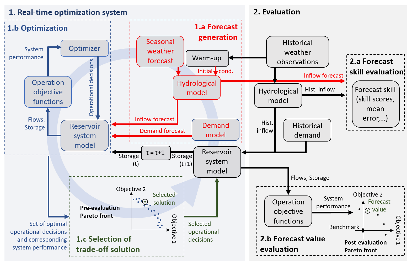
Figure 1 Diagram of the methodology used in this study to generate operational decisions using a real-time optimization system (RTOS) (left) and to evaluate its performances (right). In the evaluation step, the RTOS is nested into a closed-loop simulation, where at every time step historical data (weather, inflows and demand), along with the operational decisions suggested by the RTOS, are used to move to the next step by updating the initial hydrological conditions and reservoir storage.

1.a Forecast generation. We use a hydrological model forced by seasonal weather forecasts to generate the seasonal hydrological forecasts. The initial conditions are determined by forcing the same model by (recent) historical weather data for a warm-up period. Another model determines the future water demand during the forecast horizon. Although not tested in this study, in principle such a demand model could also be forced by seasonal weather forecasts.

1.b Optimization. This stage uses (i) a reservoir system model to simulate the reservoir storages in response to given inflows and operational decisions; (ii) a set of operation objective functions to evaluate the performance of the system, for instance, to maximize the resource availability or to minimize the operation costs; and (iii) a multi-objective optimizer to determine the optimal operational decisions. When a problem has multiple objectives, optimization does not provide a single optimal solution (i.e. a single sequence of operational decisions over the forecast horizon), but rather it provides a set of (Pareto) optimal solutions, each realizing a different trade-off between the conflicting objectives (for a definition of Pareto optimality, see, for example, Deb et al., 2002).

1.c Selection of one trade-off solution. In this stage, we represent the performance of the optimal trade-off solutions in what we call a “pre-evaluation Pareto front”. The term “pre-evaluation” highlights that these are the anticipated performances according to our hydrometeorological forecasts, not the actual performances achieved when the decisions are implemented (which are unknown at this stage). By inspecting the pre-evaluation Pareto front, the operator will select one Pareto-optimal solution according to their priorities, i.e. the relative importance they give to each operation objective. In a simulation experiment, we can mimic the operator choice by setting some rule to choose one point on the Pareto front (and apply it consistently at each decision time step of the simulation period).

2.2 Evaluation

When the RTOS is implemented in practice, the selected operational decision is applied to the real system and the RTOS used again, with updated system conditions, when a new decision needs to be made or new weather forecasts become available. If however we want to evaluate the performance of the RTOS in a simulation experiment (for instance to demonstrate the value of using a RTOS to reservoir operators) we need to combine it with the evaluation system depicted in the right part of Fig. 1. Here, the selected operational decision coming out of the RTOS is applied to the reservoir system model, instead of the real system. The reservoir model is now forced by hydrological inputs observed in the (historical) simulation period, instead of the seasonal forecasts, which enables us to estimate the actual flows and next-step storage that would have occurred if the RTOS had been used at the time. This simulated next-step storage can then be used as the initial storage volume for running the RTOS at the following time step. Once the process has been repeated for the entire period of study, we can provide an overall evaluation of the hydrological forecast skill and the performance of the RTOS, i.e. the forecast value. This evaluation (Fig. 1) consists of two stages:

2.a Forecast skill evaluation. The forecast skill is evaluated based on the differences between hydrological forecasts and observed reservoir inflows over the simulation period. For this purpose, we can calculate the absolute differences between the observed and the forecasted inflows, or we can use forecast skill scores such as the continuous ranked probability skill score (CRPSS).

2.b Forecast value evaluation. The forecast value is presented as the improvement of the system performance obtained by using the RTOS over the simulation period, with respect to the performance under a simulated benchmark operation. Notice that, because the RTOS deals with multi-objectives and hence provides a set of Pareto-optimal solutions, in principle we could run a different simulation experiment for each point of the pre-evaluation Pareto front, i.e. for each possible definition of the operational priorities. However, for the sake of simplicity, we will simulate a smaller number of relevant and well differentiated operational priorities. The simulated performances of these solutions are visualized in a “post-evaluation” Pareto front. In this Pareto front diagram, the origin of the coordinates represents the performance of the benchmark operation, and the performances of any other solution are rescaled with respect to the benchmark performance. Therefore, a positive value along one axis represents an improvement in that operation objective with respect to the benchmark, whereas a negative value represents a deterioration. When values are positive on both axes, the simulated RTOS solution dominates (in a Pareto sense) the benchmark; the further away from the origin, the more the forecast has proven valuable for decision-making. If instead one value is positive and the other is negative, then we would conclude that the forecast value is neither positive or negative because the improvement of one objective was achieved at the expense of the other.

2.3 Case study

2.3.1 Description of the reservoir system

The reservoir system used in this case study is a two-reservoir system in the south-west of the UK (schematized in Fig. 2). The two reservoirs are moderately sized, with storage capacities in the order of 20 000 000 m³ (S1) and 5 000 000 m³ (S2) (the average of UK reservoirs is 1 377 000 m³; Environment Agency, 2017). The gravity releases from reservoir S1 (u_S1,R) feed into river R and thus contribute to support downstream abstraction during low-flow periods. Pumped releases from S1 (u_S1,D) and gravity releases from reservoir S2 (u_S2,D) are used to supply the demand node D. A key operational aspect of the system is the possibility of pumping water back from river R into reservoir S1. Pumped inflows (u_R,S1) may be operated in the winter months (from 1 November till 1 April) to supplement natural inflows, provided sufficient discharge is available in the river (R). This facility provides additional drought resilience by allowing the operator to increase reservoir storage in winter to help ensure that the demand in the following summer can be met. As the pump energy consumption is costly, there is an important trade-off between the operating cost of pump storage and drought resilience.

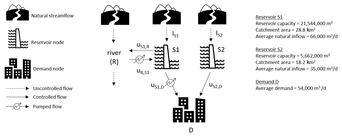
Figure 2 A schematic of the reservoir system investigated in this study to test the real-time optimization systems. Reservoir inflows from natural catchments are denoted by I, S1 and S2 are the two reservoir nodes, u denotes controlled inflows/releases, R is the river from/to which reservoir S1 can abstract and release, and D is a demand node.

The pumped storage operation is constrained by a rule curve and has operated for 11 years since 1995. The rule curve defines the storage level at which pumps are triggered. Each point on the curve is derived based on the amount of pumping that would be required to fill the reservoir by the end of the pump storage period (1 April), under the worst historical inflows' scenario. The pumping trigger is therefore risk-averse, which means there is a reasonable chance of pumping too early on during the refill period and increasing the likelihood of reservoir spills if spring rainfall is abundant. This may result in unnecessary expenditure on pumping. Informing pump operation by using seasonal forecasts of future natural inflows (I_S1 and I_S2) may thus help to reduce the volume of water pumped whilst achieving the same reservoir storage at the end of the refilling period.

2.3.2 Forecast generation

In this study we generated dynamical streamflow prediction (DSP) by forcing a lumped hydrological model, the HBV model (Bergström, 1995), with the seasonal ECMWF SEAS5 weather hindcasts (Stockdale et al., 2018; Johnson et al., 2019). The ECMWF SEAS5 hindcast dataset consists of an ensemble of 25 members starting on the first day of every month and providing daily temperature and precipitation with a lead time of 7 months. The spatial resolution is 36 km, which compared to the catchment sizes (28.8 km² for S1 and 18.2 km² for S2) makes it necessary to downscale the ECMWF hindcasts. Given the lack of clarity in the potential benefits of bias correction (Ehret et al., 2012), we will provide results of using both non-corrected and bias-corrected forecasts. The dataset of weather hindcast is available from 1981, whereas reservoir data are available for the period 2005–2016. Hence, we used the period 2005–2016 for the RTOS evaluation and the earlier data from 1981 for bias correction of the meteorological forcing. While limited, this period captures a variety of hydrological conditions, including dry winters in 2005–2006, 2010–2011 and 2011–2012, which are close to the driest period on records (1975–1976) (see more details in Fig. S1 of the Supplement). This is important because, under drier conditions, the system performance is more likely to depend on the forecast skill, and the benefits of RTOS may become more apparent (Turner et al., 2017). Daily inflows were converted to weekly inflows for consistency with the weekly time step applied in the reservoir system model.

A linear scaling approach (or “monthly mean correction”) was applied for bias correction of precipitation and temperature forecasts. This approach is simple and often provides similar results in terms of bias removal to more sophisticated approaches such as quantile or distribution mapping (Crochemore et al., 2016). A correction factor is calculated as the ratio (for precipitation) or the difference (for temperature) between the average daily observed value and the forecasted value (ensemble mean), for a given month and year. The correction factor is then applied as a multiplicative factor (precipitation) or as an additive factor (temperature) to correct the raw daily forecasts. A different factor is calculated and applied for each month and each year of the evaluation period (2005–2016). For example, for November 2005 we obtain the precipitation correction factor as the ratio between the mean observed rainfall in November from 1981 to 2004 (i.e. the average of 24 values) and the mean forecasted rainfall for those months (i.e. the average of 24×25 values, as we have 25 ensemble members). For November 2006, we recalculate the correction factor by also including the observations and forecasts of November 2005, hence taking averages over 25 values, and so forth. The rationale of this approach is to best mimic what would happen in real time, when the operator would likely access all the available past data and hindcasts for the bias correction.

As anticipated in the Introduction, the ESP is an ensemble of equiprobable weekly streamflow forecasts generated by the hydrological model (HBV in our case) forced by meteorological inputs (precipitation and temperature) observed in the past. For consistency with the bias correction approach used for the ECMWF SEAS5 hindcasts, we produce the ESP using meteorological observations from 1981 until the year before the simulated decision time step. This leads to producing an ensemble of increasing size (from 24 to 35 members) but roughly similar to the ECMWF ensemble size (25 members).

2.3.3 Optimization: reservoir system model, objective functions and optimizer

The reservoir system dynamics is simulated by a mass balance model implemented in Python. The simulation model is linked to an optimizer to determine the optimal scheduling of pumping (u_R,S1) and release (u_S1,D and u_S2,D) decisions. For the optimizer we use the NSGA-II multi-objective evolutionary algorithm (Deb et al., 2002) implemented in the open-source Python package Platypus (Hadka, 2015). We set two operation objectives for the optimizer: to minimize the overall pumping energy cost and to maximize the water resource availability at the end of the pump storage period. The pumping cost is calculated as the sum of the weekly energy costs associated with pumped inflows and pumped releases (u_R,S1 and u_S1,D) over the optimization period. The resource availability is the mean storage volume in S1 and in S2 at the end of the optimization period (1 April). When optimization is run against a forecast ensemble, the two objective functions are evaluated against each ensemble member, and the average is taken as the final objective function value. The gravity releases from S1 (u_S1,R) are not considered to be decision variables, and they are set to the observed values during the period of study. This choice is unlikely to have important implications on the optimization results because u_S1,R on average represents only 15 % of the total releases from S1 ($u_{\mathrm{S}\mathrm{1},\mathrm{D}}+u_{\mathrm{S}\mathrm{1},\mathrm{R}}$). Also, we assume that future water demands are perfectly known in advance and set them to the sum of the observed releases from S1 (u_S1,D) and S2 (u_S2,D) for the period of study. This simplification is reasonable for our case study as the water demand is fairly stable and predictable in winter, and it enables us to focus on the relationship between skill and value of the seasonal hydrological forecasts while assuming no error in demand forecasts. More details about the reservoir simulation model and the optimization problem are given in the Supplement.

2.3.4 Selection of the trade-off solution

We use five different rules for the selection of the trade-off solution from the pre-evaluation Pareto front (see Fig. 1) and apply them consistently at each decision time step of the simulation period. The five rules correspond to five different scenarios of operational priorities. They are as follows: (1) resource availability only (rao), which assumes that the operator consistently selects the extreme solution that delivers the largest improvement in resource availability; (2) resource availability prioritized (rap), which selects the solution delivering the 75 % percentile in resource availability increase; (3) balanced (bal), which selects the solution delivering the median improvement in resource availability; (4) pumping savings prioritized (psp), which selects the solution delivering the 75 % percentile in energy cost reductions; and (5) pumping savings only (pso), which selects the best solution for energy saving.

2.3.5 Forecast skill evaluation

We use two metrics, a skill score and the mean error, to evaluate the quality of the hydrological forecasts over our simulation period.

A skill score evaluates the performance of a given forecasting system with respect to the performance of a reference forecasting system. As a measure of performance, we use the continuous ranked probability score (CRPS) (Brown, 1974; Hersbach, 2000). The CRPS is defined as the distance between the cumulative distribution function of the probabilistic forecast and the empirical distribution of the corresponding observation. At each forecasting step, the CRPS is thus calculated as

$${\displaystyle }\mathrm{CRPS}\left(p\left(x\right)I^{\mathrm{Obs}}\right)=\int (p\left(x\right)-H\left(x<I^{\mathrm{Obs}}\right){)}^{\mathrm{2}}\mathrm{d}x,$$

where p(x) represents the distribution of the forecast, I^Obs is the observed inflow (m³) and H is the empirical distribution of the observation, i.e. the step function which equals 0 when x < I^Obs and 1 when x > I^Obs. The lower the CRPS, the better the performance of the forecast. In this study weekly forecast and observation data were used to compute individual CRPS values. The skill score is then defined as

$${\displaystyle }\mathrm{CRPSS}=\mathrm{1}-{\displaystyle \frac{{\mathrm{CRPS}}^{\mathrm{Sys}}}{{\mathrm{CRPS}}^{\mathrm{Ref}}}}.$$

When the skill score is higher (lower) than zero, the forecasting system is more (less) skilful than the reference. When it is equal to zero, the system and the reference have equivalent skill. Following the recommendation by Harrigan et al. (2018), we used ensemble streamflow prediction (ESP) as a hard-to-beat reference, which is more likely to demonstrate the “real skill” of the hydrological forecasting system (Pappenberger et al., 2015) and the added performance of dynamic weather forecasts.

The mean error measures the difference between the forecasted and the observed inflows (at monthly scale). The mean error is negative when the forecasts tend to underestimate the observations and positive when the forecasts overestimate the observations. The mean error for a given forecasting step and lead time T (months) is

$${\displaystyle }\mathrm{mean}\mathrm{error}={\displaystyle \frac{\mathrm{1}}{M}}\sum _{m=\mathrm{1}}^M\left({\displaystyle \frac{\mathrm{1}}{T}}\sum _{t=\mathrm{1}}^T\left(I_{t,m}^{\mathrm{Sys}}-I_t^{\mathrm{Obs}}\right)\right),$$

where I is the inflow (m³), t is the time step (months) and M the total number of members (m) of the ensemble.

2.3.6 Forecast value evaluation and definition of the benchmark operation

To evaluate the value of the hydrological forecasts, we compared the simulated performance of the RTOS informed by these forecasts with the simulated performance of a benchmark operation. The benchmark mimics common practices in reservoir operation in the UK, whereby operational decisions are made against a worst-case scenario – a repeat of the worst hydrological drought on records (1975–1976). This comparison enables us to show the potential benefits of using seasonal forecast with respect to the current approach. We simulate the benchmark operation using similar steps as in the RTOS represented in Fig. 1 but with three main variations. First, instead of seasonal weather forecasts, we use the historical weather data recorded in November 1975–April 1976 (the worst drought on records). Second, the optimizer determines the optimal scheduling of reservoir releases (u_S1,D and u_S2,D) but not that of pumped inflows (u_R,S1). Instead, these are determined by the rule curve applied in the current operation procedures. Specifically, if at the start of the week the storage level in S1 is below the storage volume defined by the rule curve for that calendar day, the operation triggers the pumping system during that week (we assume that the triggered pumped inflow is equal to the maximum pipe capacity). Third, the optimizer only aims at minimizing pumping costs, whereas the resource availability objective is turned into a constraint; i.e. the mean storage volume of the two reservoirs must be maximum by the end of the pump storage period (1 April), and no trading off with pumping costs' reduction is allowed.

3 Results

3.1 Forecast skills

First, we analyse the skill of DSP hydrological forecasts. Figure 3a shows the average CRPSS at different time steps within the pump storage period (November to April) before (red) and after (blue) bias correction of the meteorological forecasts. We compute the average CRPSS for a given time step by averaging the CRPSS of all the forecasts used from that time step to the end of the pump storage window (1 April). For instance, the average forecast skill on 1 January is obtained by averaging the CRPSS values of the hydrological forecasts for the periods 1 January–1 April (3 months' lead time), 1 February–1 April (2 months) and 1 March–1 April (1 month). This aims to represent the average skill available to the reservoir operator for managing the system until the end of the pump storage period.

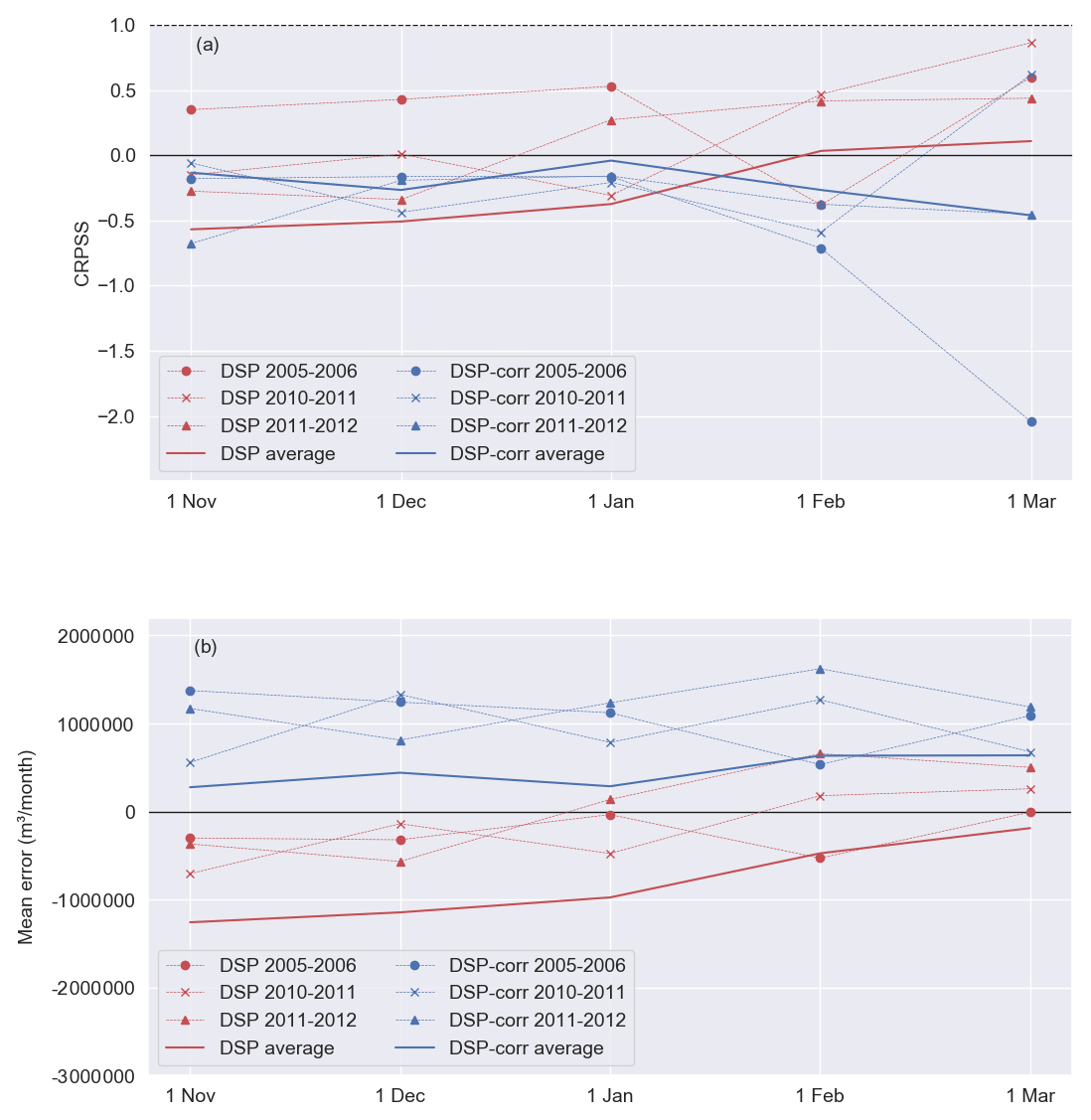
Figure 3 Skill of the hydrological forecast ensemble (inflow to reservoir S1) during the pumping licence window (1 November–1 April) measured by the CRPSS (a) and the mean error (b). For each time step, the skill is averaged over all the forecasts available from that moment to the end of the pumping window (1 April). Red lines represent the skill without bias correction of the meteorological forcing (ECMWF seasonal forecasts), and blue lines represent the skill after bias correction. Solid lines represent the average skill over the period 2005–2016, while circles, crosses and triangles represent the skill in three particularly dry winters (November–April). CRPSS = 1 corresponds to a perfect forecast, and CRPSS = 0 corresponds to a forecast that has no skill with respect to the benchmark (ESP).

Before bias correction, the average skill score is positive; i.e. the forecast is more skilful than the benchmark (ESP), only in February and March, when the forecast lead time is 1 or 2 months (solid red line). The CRPSS is higher than average in the three driest winters, i.e. 2005–2006, 2010–2011 and 2011–2012 (dashed lines). If we compare DSP to DSP-corr (red and blue solid lines), we see that bias correction deteriorates the average skill scores in February and March (lead times of 1 and 2 months), while it improves them in the previous months (when lead times are longer: 3, 4 and 5 months). In all cases though, the CRPSS values are negative; i.e. after bias correction the forecast is less skilful than the benchmark (ESP). The same happens in the driest years (dashed lines), for which bias correction mostly deteriorates the skill score.

Figure 3b shows the average mean error of the forecasts at different time steps (similarly to the CRPSS). It shows that DSP systematically underestimates the inflows (i.e. mean errors are negative) but less so in the three driest winters. After bias correction (DSP-corr), this systematic underestimation turns into a systematic overestimation. Also, the average mean error is lower for shorter lead times (i.e. in February and March), though not as much in the driest years.

In summary, we can conclude that bias correction does not seem to produce an improvement in the forecast skill for our observation period. On the other hand, what we find in our case study is a clear signal of bias correction turning negative mean errors (inflow underestimation) into positive errors (overestimation). So, while the magnitude of errors stays relatively similar, the sign of those errors changes. We will go back to this point later on, when analysing the skill–value relationship.

3.2 Forecast value

The forecast value is presented here as the simulated system performance improvement, i.e. increase in resource availability and in pumping cost savings, with respect to the benchmark operation.

3.2.1 Effect of operational priority scenario and forecast product on the forecast value

We start by analysing the average forecast value over the simulation period 2005–2016 (Fig. 4) for the three seasonal forecast products (DSP, DSP-corr and ESP) and the perfect forecast, under five operational policy scenarios (rao: resource availability only; rap: resource availability prioritized; bal: balanced; psp: pumping savings prioritized; and pso: pumping savings only).

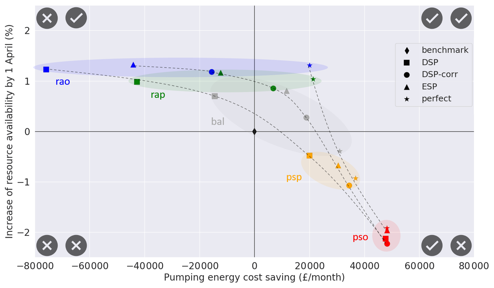
Figure 4 Post-evaluation Pareto fronts representing the average system performance improvement (over period 2005–2016) of the real-time optimization system during the pumping licence window (1 November–1 April) with respect to the benchmark (black diamond), using four forecast products: non-corrected forecast ensemble (DSP), bias-corrected forecast ensemble (DSP-corr), ensemble streamflow prediction (ESP) and perfect forecast. For each of the four forecast products, five scenarios of operational priorities are represented: resource availability only (rao; in blue), resource availability prioritized (rap; in green), balanced (bal; in grey), pumping savings prioritized (psp; in green) and pumping savings only (pso; in red). For visualization purposes, the coloured circles group points under the same operational priority scenario, and the dashed lines link points using the same forecast product. The pumping energy cost is calculated as the sum of the energy costs associated with pumped inflows and pumped releases and the resource availability as the mean storage volume in both reservoirs (S1 and S2) at the end of the optimization period. Both objective values are rescaled with respect to the performances of the benchmark operation.

Firstly, we notice in Fig. 4 that the monthly pumping energy cost savings vary widely with the operational priority. The range of variation depends on the forecast type, going from GBP 20 000 to GBP 48 000 for the perfect forecast and from GBP −77 000 to GBP 48 000 for DSP, DSP-corr and ESP. For all forecast products, the improvement in resource availability shows lower variability, with an improvement of less than +2 % (of the mean storage volume in S1 and in S2 at the end of the optimization period) for rao and a deterioration of −2 % for pso. While this seems to suggest a lower sensitivity of the resource availability objective, variations of a few percent points in storage volume may still be important in critically dry years.

As for the forecast value, we find that the perfect forecast brings value (i.e. a simultaneous improvement of both objectives) in the two scenarios that prioritize the increase in resource availability (rao and rap), DSP brings no value in any scenarios, DSP-corr has a positive value in the rap and bal scenario and ESP in the bal only. In other words, real-time optimization based on seasonal forecasts can outperform the benchmark operation, but whether this happens depends on both the forecast product being used and the operational priority.

An interesting observation in Fig. 4 is that the distance in performance between using perfect forecasts and real forecasts (DSP, DSP-corr, ESP) is very small under scenarios that prioritize energy savings (bottom-right quadrant) and much larger under scenarios prioritizing resource availability (top quadrants). This indicates a stronger skill–value relationship under the latter scenarios; i.e. improvements in the forecast skill are more likely to produce improvements in the forecast value if resource availability is the priority.

Last, if we compare DSP with DSP-corr we see that the effect of bias-correcting the meteorological forcing is mainly a systematic shift to the right along the horizontal axis, i.e. an improvement in energy cost savings at almost equivalent resource availability. Thanks to this shift, in the scenario that prioritizes resource availability (rap), DSP-corr outperforms ESP. In fact, using DSP-corr is a win–win situation with respect to the benchmark (i.e. the rap performance falls in the top-right quadrant in Fig. 4), while using ESP is not, as it improves the resource availability at the expense of pumping energy savings (i.e. producing negative savings).

3.2.2 Effect of the forecast ensemble size on the forecast value

We now analyse the effect that different characterizations of the forecast uncertainty have on the DSP-corr forecast value. We start with the extreme case when uncertainty is not considered at all in the real-time optimization, i.e. when we take the mean value of the DSP-corr forecast ensemble and use it to drive a deterministic optimization. The results are reported in Fig. 5, which shows that the solution space shrinks to the bottom-right quadrant, and, no matter the decision maker priority, the deterministic forecast only produces energy savings at the expense of reducing the resource availability. Notice that while this may still be acceptable in the scenarios that prioritize energy savings (pso and psp), in the scenarios where resource availability is optimized individually (rao) or prioritized (rap), the fact that this objective is worse than in the benchmark means that using the deterministic forecast has effectively no value.

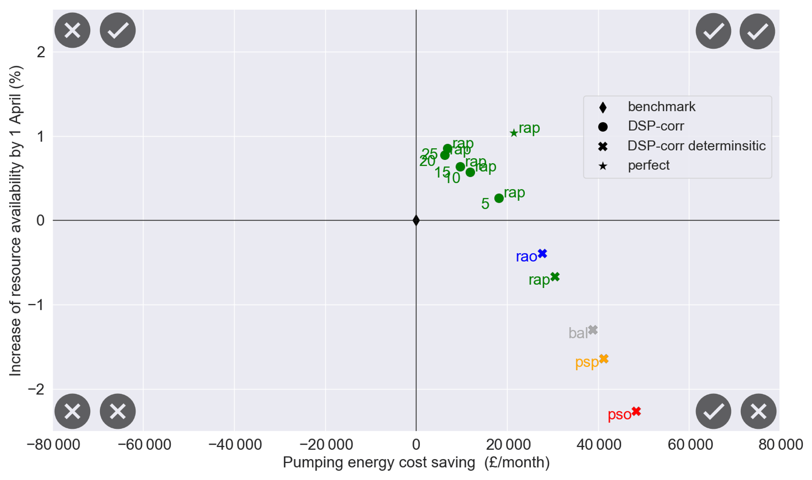
Figure 5 Post-evaluation Pareto fronts representing the average system performance (over period 2005–2016) of the real-time optimization system during the pumping licence window (1 November–1 April) with respect to the benchmark (black diamond), using the bias-corrected forecast ensemble (DSP-corr) with different ensemble size and the mean of the forecast ensemble (DSP-corr deterministic). For practical purposes, only the resource availability prioritized scenario (rap) is represented for the DSP-corr. The annotation numbers refer to the ensemble size.

We also consider intermediate cases where optimization explicitly considers the forecast uncertainty (i.e. it is based on the average value of the objective functions across a forecast ensemble), but the size of the ensemble varies between 5 and 25 members (the original ensemble size). For clarity of illustration, we focus on the resource availability prioritized (rap) scenario only. We choose this scenario because it seems to best reflect the current preferences of the system managers, whose priority is to maintain the resource availability while reducing pumping costs as a secondary objective. Moreover, the previous analysis (Fig. 4) has shown that the optimized rap has a larger window of opportunity for improving performance with respect to the benchmark and could potentially improve both operation objectives if the forecast skill was perfect.

For each chosen ensemble size, we randomly choose 10 replicates of that same size from the original ensemble, then we run a simulation experiment using each of these replicates and finally average their performance. Results are again shown in Fig. 5. For a range of 10 to 20 ensemble members, the forecast value remains relatively close to the value obtained by considering the whole ensemble (25 members). However, if only five members are considered, the resource availability is definitely lower and cost savings higher, so that the trade-off that is actually achieved is different from the one that was pursued (i.e. to prioritize resource availability). Notice that the extreme case of using one member, i.e. the deterministic forecast case (green cross in Fig. 5), further exacerbates this effect of “achieving the wrong trade-off” as resource availability is even lower than in the benchmark.

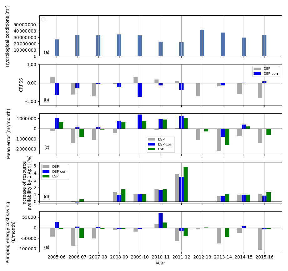
Figure 6 Year-by-year (a) hydrological conditions (total observed inflows + initial storage) and forecast skills of the meteorological forcing: (b) CRPSS and (c) mean error. (d) Increase of resource availability and (e) pumping energy cost savings of the real operation system informed by the dynamical streamflow prediction (DSP), the bias-corrected dynamical streamflow prediction (DSP-corr) and the ensemble streamflow prediction (ESP) for the resource availability prioritized (rap) scenario. Please note that ESP is not shown in (b) as it is the CRPSS benchmark.

3.2.3 Year-by-year analysis of the forecast value

Last, we investigate the temporal distribution of the forecast skill and value (i.e. increased resource availability and energy cost savings) along the simulation period and compare it to the hydrological conditions observed in each year (Fig. 6). The hydrological conditions are the sum of the initial storage value and the total inflows during the optimization period, hence enabling us to distinguish dry and wet years. Again, for the sake of simplicity we focus on the simulation results in the most relevant priority scenario of resource availability priority (rap). First, we observe that 2 specific years play the most important role in improving the system performance with respect to the benchmark: 2010–2011 for pumping cost savings (Fig. 6e) and 2011–2012 for resource availability (Fig. 6d). These years correspond to the driest conditions in the period of study (see Fig. 6a and the Supplement for further analysis of the inflow data) but not to the highest forecast skills either quantified with the CRPSS or mean error (Fig. 6b and c). In general, the temporal distribution of the average yearly forecast skill does not show any correspondence with the yearly forecast value. When comparing DSP-corr with DSP (blue and grey bars), we observe that they perform similarly in terms of resource availability, but DSP-corr performs better for energy savings. This difference was observed already when looking at average performances over the simulation period (Fig. 4) and can be related to the change in sign of forecasting errors induced by the bias correction of the meteorological forcing (Fig. 3b). In fact, without bias correction, reservoir inflows tend to be underestimated, which leads the RTOS to pump more frequently and often unnecessarily (e.g. in 2005–2006, 2006–2007 and 2007–2008). With bias correction, instead, inflows tend to be overestimated, and the RTOS uses pumping less frequently. Interestingly, the reduction in pumping still does not prevent the resource availability from being improved with respect to the benchmark. This is achieved by the RTOS through a better allocation of pump and release volumes over the optimization period. When comparing DSP-corr with ESP, we find that the largest improvements are gained in the same years by both products, i.e. in the driest ones. As already emerged from the analysis of average performances (Fig. 4), we see that ESP achieves slightly better resource availability than DSP-corr but with less pumping cost savings. ESP in particular seems to produce “unnecessary” pumping costs in 2006–2007, 2011–2012 and 2013–2014, where DSP-corr achieves a similar resource availability (Fig. 6d) at almost no cost (Fig. 6e). It must be noted that for the ESP approach, these 3 specific years, 2006–2007, 2011–2012 and 2013–2014, play the most important role in decreasing the pumping energy cost savings with respect to the benchmark.

4 Discussion

Our study provides some insights into the complex relationship between forecast skill and its value for decision-making. Although these findings may be dependent on the case study and time period that was available for the analysis, they still enable us to draw some more general lessons that could be useful also beyond the specific case investigated here.

First, we found that evaluating the usefulness of bias correction, and in particular linear scaling of the meteorological forcing, is less straightforward than possibly expected. Our results show that, on average, bias correction does not improve the DSP forecast skill (as measured by the CRPSS and mean error) and can even deteriorate it in dry years (Fig. 3). This is because in our system DSP forecasts systematically underestimate inflows (before bias correction), which means their skill is relatively higher in exceptionally dry years and is deteriorated by bias correction. To the best of our knowledge, no previous study has reported such difference in skill for the ECMWF SEAS5 forecasts in dry years in the UK; hence we are not able to say whether our result applies to other systems in the region. However, the result points at a possible intrinsic contradiction in the very idea of bias-correcting based on climatology. In fact, by pushing forecasts to be more like climatology, bias correction may reduce the “good signal” that may be present in the original forecast in years that will indeed be significantly drier (or wetter) than climatology. As exceptional conditions are likely the ones when water managers can extract more value from forecasts, the argument that bias correction ensures average performance at least equivalent to climatology or ESP (e.g. Crochemore et al., 2016) may not be very relevant here. We would conclude that more studies are needed to investigate the benefits of bias correction when seasonal hydrological forecasts are specifically used to inform water resource management.

While we could not find an obvious and significant improvement of forecast skill after bias correction, we found a clear increase in forecast value (Fig. 4). The RTOS based on bias-corrected DSP considerably reduces pumping costs with respect to the original DSP while ensuring similar resource availability. A consequence of this is that decision maker priorities rap (resource availability prioritized) and bal (balanced) dominate (in a Pareto sense) the benchmark. We explained this reduction in pumping costs by the fact that bias correction changed the sign of the forecasting errors – from a systematic underestimation of inflows to a systematic overestimation. While this change is again case-specific, a general implication is that not all forecast errors have the same impact on the forecast value, and thus not all skill scores may be equally useful and relevant for water resource managers. For example, in our case a score that is able to differentiate between overestimation and underestimation errors, such as the mean error, seems more adequate than a score such as the CRPSS, which is insensitive to the error sign. This said, our results overall suggest that inferring the forecast value from its skill may be misleading, given the weak relationship between the two (at least as long as we use skill scores that are not specifically tailored to water resource management). Running simulation experiments of the system operation, as done in this study, can shed more light on the value of different forecast products.

While we found a weak relationship between forecast skill and value, we found that forecast value is more strongly linked to hydrological conditions (Fig. 6). As expected, a forecast-based RTOS system is particularly useful in dry years, where we find most of the gains with respect to the benchmark operation (Fig. 6). This is consistent with previous studies for water supply system, e.g. Turner et al. (2017). In our case study,the RTOS not only improves resource availability but also reduces pumping costs because, in the drier years, storage levels are more likely to cross the rule curve and trigger pumping in the benchmark operation.

In light of the pre-processing costs of seasonal weather forecasts, it is interesting to discuss whether their use is justified with respect to a possibly simpler-to-use product such as ESP. While weather forecast centres are increasingly reducing the pre-processing costs by facilitating access to their seasonal weather forecast datasets, preparation of the forecasts, including bias correction, still needs a considerable level of expertise. This is not only because tools for bias correction are not readily available but also because deciding whether to apply bias correction in the first place may be not obvious, as shown in this case study, and expertise is needed to select and apply an adequate bias correction method. In this study, we found ESP to be a hard-to-beat reference, not only in terms of skill (as previously found by others, e.g. Harrigan et al., 2018) but also in terms of forecast value (Fig. 4). In fact, while using DSP-corr delivers higher energy savings with respect to ESP at least in the most relevant operating priority scenario (the rap scenario; see Fig. 6), it is difficult to argue whether these cost savings are large enough to justify the use of DSP-corr or whether water managers may fall back on using simpler ESP.

One aspect for which our results instead point to a univocal and clear conclusion is in the importance of explicitly considering forecast uncertainty (Fig. 5). In fact, the RTOS outperforms the current operation when using ensemble forecasts, but it does not if uncertainty is removed and the system is optimized against the ensemble mean. In this case, in fact, DSP-corr improves energy savings, but it decreases the resource availability under all operational priority scenarios, including those where resources availability should be prioritized. This is in line with previous results obtained using short-term forecasts for flood control (Ficchì et al., 2016), which found that consideration of forecast uncertainty could largely compensate the loss in value caused by forecast errors, hydropower generation (Boucher et al., 2012) and multi-purpose systems (Yao and Georgakakos, 2001). It is also consistent with previous results by Anghileri et al. (2016), who did not find significant value in seasonal forecasts while using a deterministic optimization approach (they did not explore the use of ensembles though).

Finally, we tried to investigate whether we could evaluate the effect of the ensemble size on the value of the uncertain forecasts. We found that in our case study we could reduce the number of forecast members down to about 10 (from the original size of 25) with limited impact on the forecast value (Fig. 5). This is important for practice because by reducing the number of forecast members one can reduce the computation time of the RTOS. While we cannot say if such an “optimal” ensemble size would apply to other systems, we would suggest that future studies could look at how the quality of the uncertainty characterization impacts the forecast value and whether a “minimum representation of uncertainty” exists that ensures the most effective use of forecasts for water resource management.

From the UK water industry perspective, we hope our results will motivate a move away from the deterministic (worst-case scenario) approach that often prevails when using models to support short-term decisions and a shift towards more explicit consideration of model uncertainties. Such a move would also align with the advocated use of “risk-based” approaches for long-term planning (Hall et al., 2012; Turner et al., 2016; UKWIR, 2016a, b), which have indeed been adopted by water companies in the preparation of their Water Resource Management Plans (Southern Water, 2018; United Utilities, 2019). The results presented here, and in the above cited studies, suggest that greater consideration of uncertainty and trade-offs would also be beneficial in short-term production planning.

4.1 Limitations and perspective for future research and implementation

Our study is subject to a range of limitations that should be kept in mind when evaluating our results. First, the current (and future) skill of seasonal meteorological forecasts varies spatially across the UK depending on the influence of climate teleconnections and particularly the NAO. Given that our case study is located in the south-west of the UK, where the NAO influence has been found to be stronger than in the east (Svensson et al., 2015), our simulated benefits of using DSP seasonal forecasts may be particularly optimistic. Second, the general validity of the results is limited by the relatively short period (2005–2016) that was available for historical simulations and which may be insufficient to fully characterize the variability of hydrological conditions and hence accurately estimate the system's performances (see, for example, the discussion in Dobson et al., 2019). Hence, we aim at continuing the evaluation of the RTOS over time as new seasonal forecasts and observations become available. Another limitation is that we used the observed water demand, hence implicitly assuming that operators know in advance the demand values for the entire season with full certainty.

Future studies should extend the testing of the RTOS over a longer time horizon and evaluate the influence of errors in forecasting water demand. To improve our understanding of the forecast skill–value relationship and the benefits of bias correction, it would also be interesting to test the sensitivity of our results to the use of different skill scores and bias correction methods. The higher skill of DSP forecast for 1- and 2-month lead times suggests that combining DSP and ESP forecasts (for instance using the former for the first 2 months and the latter for the rest of the forecast horizon) may also be a promising approach to explore in future studies. Finally, another direction for future improvement is the refinement of the optimization approach, given that here we used a simpler but sub-optimal method (see further discussion in the Supplement).

The Python code developed for this study has been implemented in a set of interactive Jupyter Notebooks, which we have now transferred to the water company in charge of the pumped storage decisions. A generic version of this code for applying our methodology to other reservoir systems is available as part of the open-source toolkit iRONS (https://github.com/AndresPenuela/iRONS, last access: 10 December 2020) (Peñuela and Pianosi, 2020a). This toolkit aims at helping to overcome some of the current barriers to the implementation of forecast-informed reservoir operation systems, by providing better “packaging” of model results and their uncertainties, enabling the interactive involvement of decision makers and creating a standard and formal methodology to support model-informed decisions (Goulter, 1992). Besides supporting the specific decision-making problem faced by the water company involved in this study, through this collaboration we aim at evaluating more broadly how effective our toolkit is to promote knowledge transfer from the research to the professional community and gain a better understanding of how decision makers view forecast uncertainty, the institutional constraints limiting the use of this information (Rayner et al., 2005) and the most effective ways in which forecast uncertainty and simulated system robustness can be represented.

5 Conclusions

This work assessed the potential of using a real-time optimization system informed by seasonal forecasts to improve reservoir operation in a UK water supply system. While the specific results are only valid for the studied system, they enable us to draw some more general conclusions. First, we found that the use of seasonal forecasts can improve the efficiency of reservoir operation but only if the forecast uncertainty is explicitly considered. Uncertainty is characterized here by a forecast ensemble, and we found that the performance improvement is maintained also when the forecast ensemble size is reduced up to a certain limit. Second, while dynamical streamflow prediction (DSP) generated by numerical weather predictions provided the highest value in our case study (under a scenario that prioritizes water availability over pumping costs), still ensemble streamflow prediction (ESP), which is more easily derived from observed meteorological conditions in previous years, remains a hard-to-beat reference in terms of both skill and value. Third, the relationship between the forecast skill and its value for decision-making is complex and strongly affected by the decision maker priorities and the hydrological conditions in each specific year. It must be noted that in practice the decision-making priorities are not solely related to the selection of a specific Pareto-optimal solution but in the first place to the methodology, i.e. the “risk” taken in using something other than the worst-case scenario approach and in applying bias correction of the meteorological forcing or not. We also hope that the study will stimulate further research towards better understanding the skill–value relationship and finding ways to extract value from forecasts in support of water resource management.