Stochastic simulation of streamflow and spatial extremes: a continuous, wavelet-based approach

Stochastically generated streamflow time series are used for various water management and hazard estimation applications. They provide realizations of plausible but as yet unobserved streamflow time series with the same temporal and distributional characteristics as the observed data. However, the representation of non-stationarities and spatial dependence among sites remains a challenge in stochastic modeling. We investigate whether the use of frequency-domain instead of time-domain models allows for the joint simulation of realistic, continuous streamflow time series at daily resolution and spatial extremes at multiple sites. To do so, we propose the stochastic simulation approach called Phase Randomization Simulation using wavelets (PRSim.wave) which combines an empirical spatio-temporal model based on the wavelet transform and phase randomization with the flexible four-parameter kappa distribution. The approach consists of five steps: (1) derivation of random phases, (2) fitting of the kappa distribution, (3) wavelet transform, (4) inverse wavelet transform, and (5) transformation to kappa distribution. We apply and evaluate PRSim.wave on a large set of 671 catchments in the contiguous United States. We show that this approach allows for the generation of realistic time series at multiple sites exhibiting short- and long-range dependence, non-stationarities, and unobserved extreme events. Our evaluation results strongly suggest that the flexible, continuous simulation approach is potentially valuable for a diverse range of water management applications where the reproduction of spatial dependencies is of interest. Examples include the development of regional water management plans, the estimation of regional flood or drought risk, or the estimation of regional hydropower potential. Highlights.

1. Stochastic simulation of continuous streamflow time series using an empirical, wavelet-based, spatio-temporal model in combination with the parametric kappa distribution.

2. Generation of stochastic time series at multiple sites showing temporal short- and long-range dependence, non-stationarities, and spatial dependence in extreme events.

3. Implementation of PRSim.wave in R package PRSim: Stochastic Simulation of Streamflow Time Series using Phase Randomization.

1 Introduction

Stochastic models are used to generate long time series or large event sets showcasing the full variability of a phenomenon. In hydrology, we use stochastically generated time series or event sets to refine water management plans, to get a better idea of potential reservoir inflows, or to develop suitable adaptation strategies for droughts and floods. If the focus is on such extreme events, event-based instead of continuous simulation approaches are often employed (e.g., Bracken et al., 2016; Diederen et al., 2019; Quinn et al., 2019). This strategy requires an a priori definition of extreme events and leads to a loss of temporal information, e.g., on the season of occurrence. In contrast, continuous simulation approaches allow for the simulation of time series including, but not limited to, extreme events which are provided together with their time of occurrence. Such continuous approaches enable the investigation of drought and flood characteristics going beyond magnitude and extending to timing, duration, or volume. However, the model representation of this additional information on timing adds some challenges because the temporal characteristics of the data need to be represented in addition to their distribution. These temporal characteristics include fluctuations on short and long timescales (Rajagopalan et al., 2010) and potential non-stationarities in the data (Nowak et al., 2011).

There exists a variety of continuous, stochastic modeling approaches (corresponding to discrete-time models in the stochastic literature) which differ in their capability of representing distributional and/or temporal characteristics in the data. Here, we focus on direct modeling approaches that directly simulate streamflow using a stochastic model as opposed to indirect approaches which use a hydrological model to transform stochastically generated precipitation into streamflow. The most commonly used stochastic simulation approaches belong to the two classes of parametric and nonparametric models. Parametric models include autoregressive moving average (ARMA) models and their modifications (Stedinger and Taylor, 1982; Papalexiou, 2018) and fractional Gaussian noise models (Mandelbrot, 1965) comprising fast fractional Gaussian noise models (Mandelbrot, 1971), broken line models (Mejia et al., 1972), and fractional autoregressive integrated moving average models (Hosking, 1984). Nonparametric models include kernel density estimation (Lall and Sharma, 1996; Sharma et al., 1997) and various bootstrap approaches such as simple bootstrap, moving-block bootstrap, nearest-neighbor bootstrap (Salas and Lee, 2010; Herman et al., 2016), matched-block bootstrap (Srinivas and Srinivasan, 2006), or maximum-entropy bootstrap (Srivastav and Simonovic, 2014). These parametric and non-parametric methods have different strengths and weaknesses as, e.g., discussed in Rajagopalan et al. (2010), and the representation of spatial dependence in such time-domain models is challenging. For parametric models, the number of parameters grows rapidly with the number of locations (Caraway et al., 2014) and the spatial dependence structure is similar for high-, medium-, and low-flow values, which is not the case for observed data (Sharma et al., 1997). Similarly, non-parametric approaches are not effective for multiple-site streamflow generation because of the high dimension of the problem (Nowak et al., 2010).

In contrast to most time-domain models, frequency-domain models allow for the simulation of surrogate data with the same Fourier spectra as the raw data (Theiler et al., 1992) and can easily be extended to multiple sites (Prichard and Theiler, 1994; Schreiber and Schmitz, 2000). Such methods are based on the randomization of the phases of the Fourier transform and are known as the amplitude-adjusted Fourier transform (AAFT) (Lancaster et al., 2018). They have only recently been used in hydrology for other applications besides hypothesis testing, trend detection (Radziejewski et al., 2000), and the identification of nonlinearities in time series (Schmitz and Schreiber, 1996; Kugiumtzis, 1999; Venema et al., 2006; Maiwald et al., 2008). Serinaldi and Lombardo (2017) used an iterative AAFT method to generate binary series of rainfall occurrence and non-occurrence. Brunner et al. (2019) used a phase randomization approach in combination with the flexible four-parameter kappa distribution (Hosking, 1994) to simulate continuous discharge time series including unobserved extremes. The approach is implemented in the R package Stochastic Simulation of Streamflow Time Series using Phase Randomization PRSim (Brunner and Furrer, 2019) and can be applied to both individual and multiple sites. This phase randomization approach has been shown to reproduce the distributional and temporal characteristics of the data at individual sites well (Brunner et al., 2019; Brunner and Tallaksen, 2019). However, the approach has some deficiencies when applied to multiple sites because spatial dependencies in both daily discharge and extreme events are underestimated. In addition, the approach does not allow for the consideration of non-stationarities.

In contrast to the Fourier transform, the wavelet transform allows for the representation of non-stationarities in time series (Rajagopalan et al., 2010). For a short introduction to the wavelet transform, see Sect. 2. In addition, it may help to improve the representation of spatial dependencies because it does not require a transformation to the normal distribution and back to the original, skewed distribution, which usually weakens spatial correlations (Embrechts et al., 2010). This weakening is because phase randomization preserves the cross-correlation in the normal domain but not necessarily in the domain of the original distribution as linear correlation is not invariant under nonlinear strictly increasing transformations. Because of its favorable properties, the wavelet transform has been used in stochastic time series generation in various ways. Kwon et al. (2007) proposed a wavelet-based autoregressive modeling (WARM) approach suitable for systems with a quasi-periodic long memory behavior. They used the continuous wavelet transform to decompose a time series into several statistically significant components. Each of these components was fitted using a linear autoregressive (AR) model which was subsequently used for simulation. Later, Nowak et al. (2011) adapted this WARM approach such that it can handle non-stationarities. Another possibility for handling non-stationarities is the wavelet-based time series bootstrap model introduced by Erkyihun et al. (2016) which generates wavelet-derived signal components with a block resampling approach, therefore replacing the AR component of WARM.

An alternative to these approaches where only certain signal components are modified are approaches that randomize the wavelet coefficients for all components. These approaches typically perform a discrete wavelet decomposition using real wavelet functions (as opposed to complex wavelet functions), randomize the real-valued wavelet coefficients (i.e., amplitudes), and then invert the transform to produce a new realization of a time series (Breakspear et al., 2003; Keylock, 2007; Wang et al., 2010; Lancaster et al., 2018). However, a completely random shuffling of coefficients destroys their periodicity. To overcome this drawback, Breakspear et al. (2003) used block resampling on coefficients and Keylock (2007) introduced a threshold criterion that is used to pin particular wavelet coefficients to the same position in the wavelet domain for both the original and surrogate data. Despite these workarounds, some of the long-term periodicities and/or non-stationarities may not be preserved (Breakspear et al., 2003). Using a continuous instead of discrete wavelet transform allows for the use of complex wavelet functions which provide complex-valued coefficients containing information on the phase in addition to amplitude. The use of this additional phase information in the randomization process instead of the amplitude can prevent the loss of non-stationarities. To generate non-stationary surrogate time series, Chavez and Cazelles (2019) extended the classic phase-randomized surrogate data algorithm to the time–frequency domain using a dataset of weekly measles notifications and an electroencephalographic recording. They randomized the phases resulting from the continuous wavelet transform instead of the real-valued amplitudes. This approach has the advantage of being non-parametric, avoids assumptions about the distribution and dependence structure of the data, allows for multiple realizations, and can be extended to multiple sites by randomizing the phases for multiple time series in the same way (Prichard and Theiler, 1994; Schreiber and Schmitz, 2000).

We investigate whether such a wavelet-based phase randomization approach allows for a realistic representation of spatial dependence in both continuous streamflow time series and spatial extremes. To do so, we propose a continuous wavelet-based approach for the stochastic generation of streamflow time series, hereafter referred to as PRSim.wave, which is based on the empirical spatio-temporal model used by Chavez and Cazelles (2019), i.e., wavelet-based phase randomization. This empirical approach is supposed to overcome difficulties in modeling spatial dependence over a large domain as occurs when using parametric models (Caraway et al., 2014). We combine this empirical spatio-temporal model with a parametric distribution to enable the generation of hydrological extremes exceeding the range of the observed values. By doing so, we extend the approach by Brunner et al. (2019) from the Fourier to the wavelet domain, therefore improving the representation of spatial dependencies and non-stationarities.

We implement PRSim.wave in the R package PRSim (Brunner et al., 2019) and apply and evaluate it on a large dataset of 671 catchments in the contiguous United States. Our evaluation results indicate that the flexible, continuous simulation approach can be used for a diverse range of water management applications requiring continuous discharge time series at multiple sites or for regional drought and flood hazard assessments not limited to peak magnitude or maximum deficit, but extending to event duration and volume.

2 Theoretical background

Wavelet decomposition transforms a one-dimensional time series to a two-dimensional time–frequency space (Daubechies, 1992; Torrence and Compo, 1998) using either a discrete or continuous wavelet transform. Both transforms decompose a hydrological series into a set of coefficients, representing different scales or frequency bands (Sang, 2012). The coefficients of the discrete transform are real numbers representing amplitudes. In contrast, the coefficients derived from the continuous transform have a real and an imaginary part corresponding to an amplitude and phase, respectively. This additional information on the phases makes complex wavelet functions more suitable for capturing oscillatory behavior (Torrence and Compo, 1998).

The wavelet function used for the transform should reflect the features present in the time series. Because of its smooth features, the Morlet wavelet has often been used in hydrological applications (Labat et al., 2005; Lafrenière and Sharp, 2003; Schaefli et al., 2007) and is given by (Torrence and Compo, 1998)

$$\begin{array}{}\text{(1)}& {\mathit{\psi }}_{\mathrm{0}}\left(\mathit{\eta }\right)={\mathit{\pi }}^{-\mathrm{1}/\mathrm{4}}{e}^{i{\mathit{\omega }}_{\mathrm{0}}\mathit{\eta }}{e}^{-{\mathit{\eta }}^{\mathrm{2}}/\mathrm{2}},\end{array}$$

where η is a non-dimensional time parameter, ω₀ is the non-dimensional frequency, and $i=\sqrt{-\mathrm{1}}$ is the imaginary unit. The continuous wavelet transform is defined as the convolution of a time series x_n of length n with a scaled version of ψ₀(η):

$$\begin{array}{}\text{(2)}& W_n\left(h\right)=\sum _{n^{\prime }=\mathrm{0}}^{N-\mathrm{1}}{x}_{n^{\prime }}{\mathit{\psi }}^{*}\left[{\displaystyle \frac{(n^{\prime }-n)\mathit{\delta }t}{h}}\right],\end{array}$$

where ^* indicates the complex conjugate. Varying the wavelet scale h and translating along the localized time index n allows for showing of the amplitude of certain features vs. scale and how the amplitude varies with time and scale. An inverse filter can be used to reconstruct the original time series as the sum of the real part of the wavelet transform over all scales (h₁, …, h_J):

$$\begin{array}{}\text{(3)}& x_n={\displaystyle \frac{\mathit{\delta }j\mathit{\delta }{t}^{\mathrm{1}/\mathrm{2}}}{C_{\mathit{\delta }}{\mathit{\psi }}_{\mathrm{0}}\left(\mathrm{0}\right)}}\sum _{j=\mathrm{0}}^J{\displaystyle \frac{R\left(W_n\left(h_j\right)\right)}{h_j^{\mathrm{1}/\mathrm{2}}}},\end{array}$$

where the factor ψ₀(0) removes the energy scaling, $h_j^{\mathrm{1}/\mathrm{2}}$ converts the wavelet transform to an energy density, and the factor C_δ is a constant for each wavelet function (0.776 for the Morlet wavelet).

3 Data and methods

We develop and apply the stochastic simulation approach PRSim.wave using a large-scale dataset of 671 stations in the contiguous United States (CONUS). We evaluate the approach with respect to distributional and temporal characteristics at individual sites and with respect to spatial dependencies across multiple sites in general and for floods in particular.

3.1 Study area

The 671 catchments in the United States cover a wide range of discharge regimes minimally influenced by human activity (Newman et al., 2015; Addor et al., 2017; Brunner et al., 2020b). Daily discharge data were downloaded for the period 1981–2018 from the USGS water information system (USGS, 2019) using the R package dataRetrieval (De Cicco et al., 2018).

For illustration and validation purposes, we select three regions which are distinct in terms of their hydrological regimes and their flood behavior. Flood similarity regions were determined by Brunner et al. (2020a) using hierarchical clustering (Gordon, 1999) on a distance matrix computed from the F-madogram, which is a measure of extremal dependence between pairs of stations (Cooley et al., 2006). The clustering was applied to the 671 catchments and resulted in 15 clusters, among which we selected 3 for illustration purposes: (1) catchments in the lower-elevation coastal Pacific Northwest characterized by high mean annual precipitation and a strong discharge seasonality experiencing floods mainly in December and January, (2) catchments in Texas with low mean discharge, weak seasonality, and flood occurrence in spring to fall, and (3) catchments in the Mid-Atlantic coastal plain and central Appalachian Mountains with a strong streamflow seasonality showing flood occurrence for much of the year except early–mid summer. For each of these regions, four catchments are chosen for illustration purposes (Fig. 1).

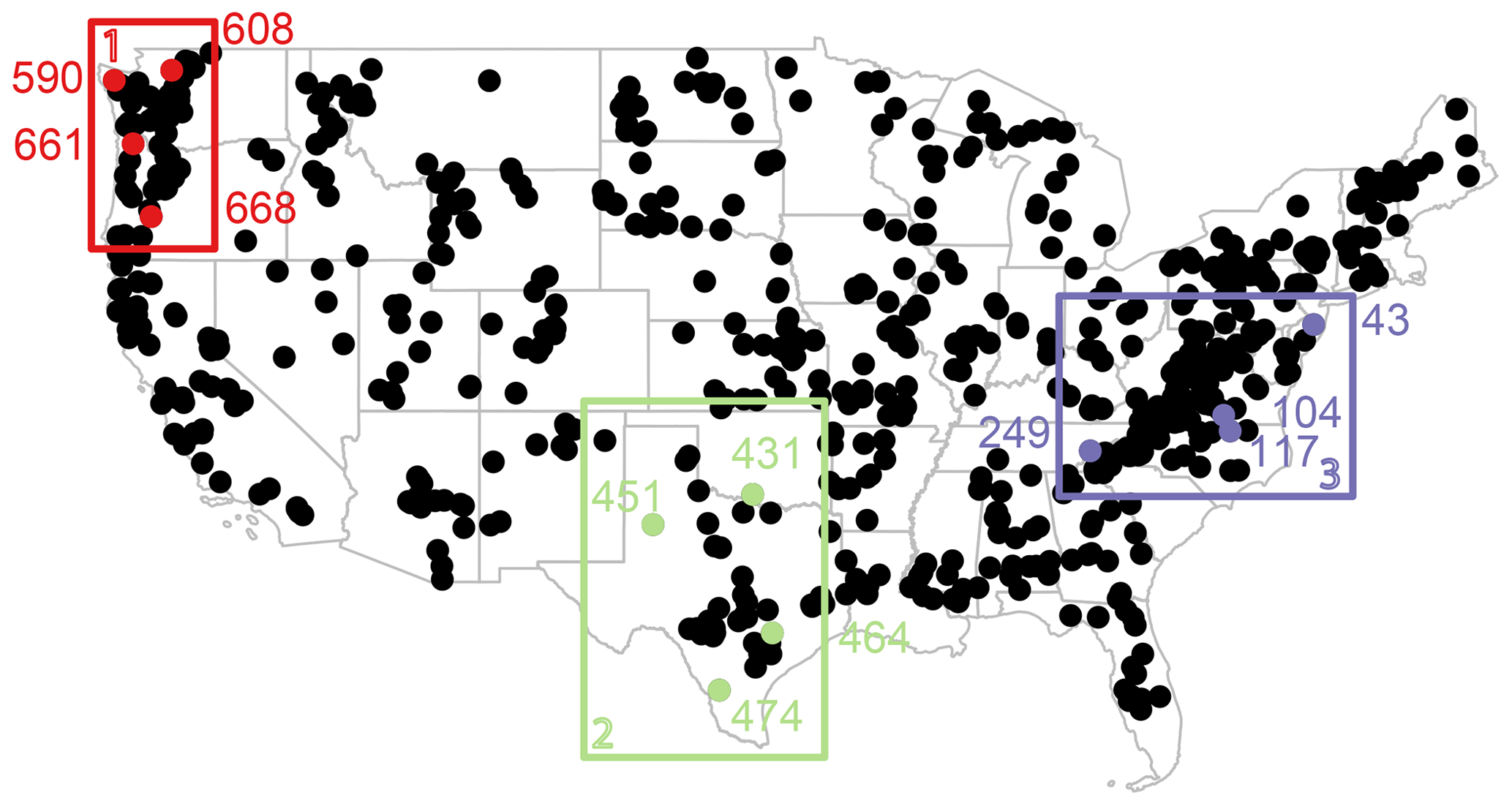
Figure 1 Location of 671 stations in the dataset and of four catchments chosen per example region: (1) Pacific Northwest (red; 590, 608, 661, and 668), (2) Texas (light green; 431, 451, 464, and 474), and (3) Mid-Atlantic (purple; 43, 104, 117, and 249).

3.2 Simulation procedure

The stochastic simulation procedure PRSim.wave for multiple sites consists of five main steps (Fig. 2), which can be run p times to generate p spatially consistent time series over n sites at daily resolution.

1. Derivation of random phases: a random discharge time series (white noise) of the same length as the input series is sampled from a normal distribution with mean 0 and standard deviation 1 (Chavez and Cazelles, 2019). We also tested the kappa distribution, which did, however, not significantly change the model performance. The wavelet transform is applied to the white noise series using the Morlet wavelet (Eq. 1) for h=100 wavelet scales; 100 scales are used as using only a few scales (e.g., 20) results in reconstructed time series that do not reflect all the necessary detail, while further increasing the number of scales no longer improves reconstruction performance. The phases of the wavelet transform are derived. These same phases are used for all the sites considered to retain spatial dependencies among sites (Prichard and Theiler, 1994; Schreiber and Schmitz, 2000).

2. Fitting of kappa distribution: the flexible four-parameter kappa distribution (Hosking, 1994) is fit to the daily values of the observed input time series using L moments. These daily distributions will be used for the transformation in Step 5 to simulate extreme values going beyond the empirical distribution. The cumulative distribution function of the kappa distribution is expressed as

   $$\begin{array}{}\text{(4)}& F\left(x\right)={\left\{\mathrm{1}-\mathit{\xi }{\left[\mathrm{1}-\mathit{\kappa }(x-\mathit{\mu })/\mathit{\sigma }\right]}^{\mathrm{1}/\mathit{\kappa }}\right\}}^{\mathrm{1}/\mathit{\xi }},\end{array}$$

   where μ is the location parameter, σ is the scale parameter which must be positive, and κ and ξ are the shape parameters (R package homtest; Viglione, 2009).

   The kappa distribution was found to be suitable for fitting observed streamflow data in US catchments (Blum et al., 2017). A suitable fit is also found for our data, as confirmed by the Kolmogorov–Smirnov and Anderson–Darling tests (Chernobai et al., 2015), which did not reject the null hypothesis at α=0.05 for most catchments. We fit a separate distribution for each day using a moving window approach to take into account seasonal differences in the distribution of daily streamflow values. To do so, we use the daily values in a 30 d window around the day of interest. This procedure guarantees a large enough sample for the parameter fitting procedure and allows for smoothly changing distributions along the year. For leap years, flows from 29 February are removed to maintain constant sample sizes across years as in Blum et al. (2017). In a few regions with many zero discharge values (e.g., some catchments in the Great Plains) fitting the kappa distribution is not possible and we therefore use the empirical distribution instead. After fitting the daily distributions, the mean discharge is subtracted from the observed discharge values to center the observations.

3. Wavelet transform: the wavelet transform (Eq. 2) is applied to the input time series using the complex-valued Morlet wavelet (Eq. 1) to derive the amplitudes for h=100 number of wavelet scales. The complex part of the wavelet transform W_n(h) comes in via the complex conjugate ^* in Eq. (2). The complex conjugate is derived using the modulus and argument, i.e., the phases of the complex numbers contained in the Morlet wavelet (Eq. 1). The wavelet coefficients W_n(h) resulting from the transform are also complex numbers, where the argument of the complex wavelet value W_n(h) corresponds to the wavelet phase.

4. Inverse wavelet transform: reconstruction of the series in the time domain by using the inverse wavelet transform (Eq. 3) combining the random phases derived in Step 1 and the amplitudes derived in the previous step. During back transformation in Eq. (3), the phases come back in when deriving the real part at each scale h through R(W_n(h_j)).

5. Transformation to kappa distribution: the simulated values are transformed to the kappa domain using the fitted daily kappa distributions from Step 2. For each day, a random sample is generated from the fitted, daily kappa distribution. Negative simulated values are replaced by 0. The simulated values are replaced by the values generated from the kappa distribution using rank-ordering. This procedure is repeated for each day in the year.

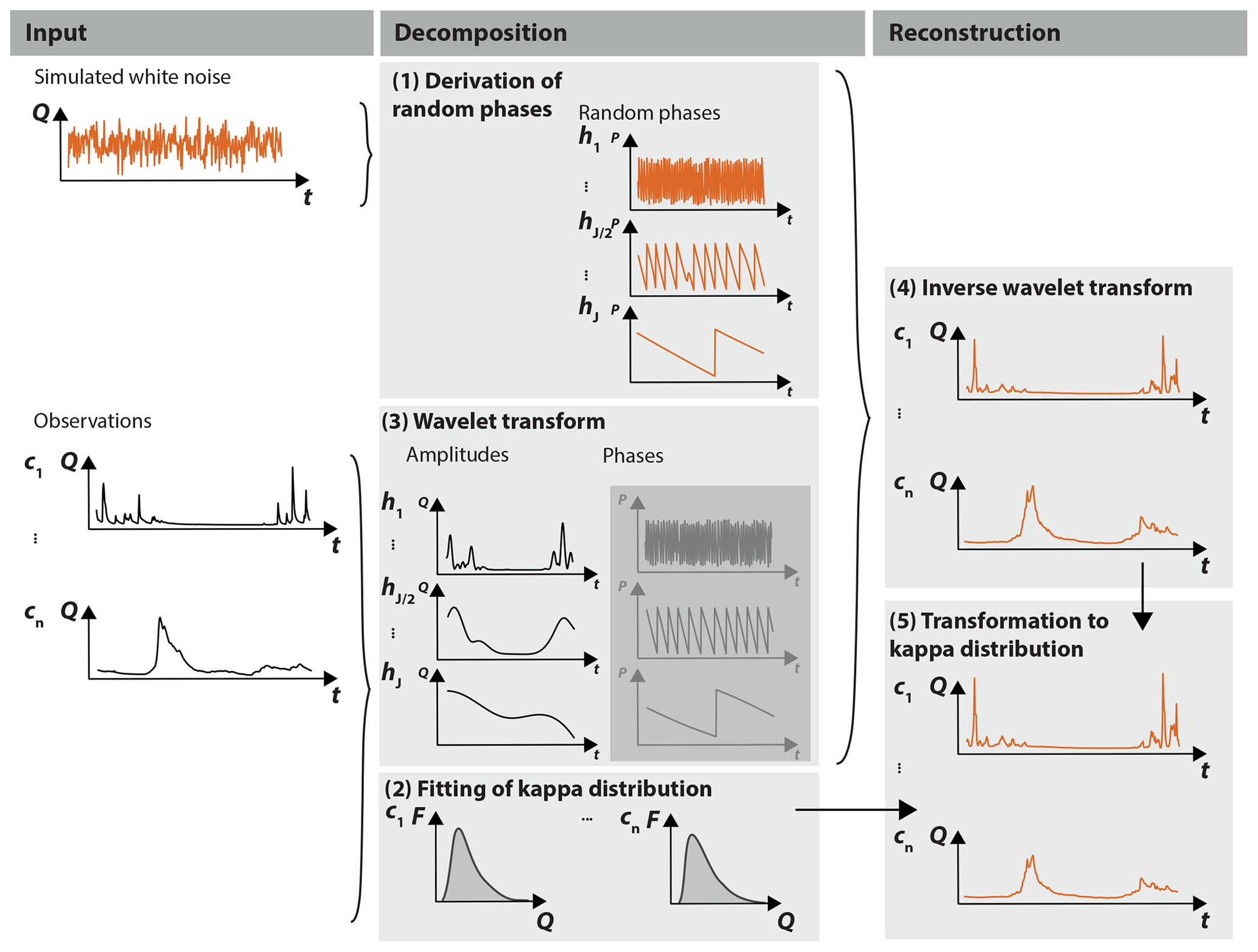
Figure 2 Illustration of stochastic simulation approach PRSim.wave: (1) derivation of random phases which are uniformly distributed over the range of −π to π, using a white noise time series to be used for the simulation at all stations; for each station: (2) fitting of kappa distribution to the observed streamflow time series using L moments; (3) wavelet transform to derive the amplitudes and phases of the time series; (4) inverse wavelet transform recomposing a time series using the random phases from Step 1 in combination with the amplitudes of Step 3; and (5) transformation to the kappa distribution using the kappa distribution fitted in Step 2. Steps 1–5 are repeated p times to generate p time series.

Step 1 is run only once per iteration to maintain spatial dependencies in the data, while Steps 2–5 are run for each station separately.

3.3 Evaluation

We run the stochastic simulation algorithm for the 671 catchments in the dataset n=100 times to generate 100 time series of the same length as the observed time series, i.e., 38 years. We look at (1) individual sites to evaluate the general distributional and temporal correlation characteristics as well as the reproduction of high and low flows; (2) three sets of four stations each to evaluate the spatial consistencies in daily discharge and floods: Pacific Northwest, Texas, and Mid-Atlantic (Fig. 1); and (3) at the set of 671 catchments to evaluate spatial consistencies in floods across large scales.

The evaluation at individual sites encompasses a comparison of observed and simulated distributional and temporal discharge characteristics. The distributional characteristics considered are the mean annual hydrograph showing variation of flow with season, 3 years of daily data illustrating the overall behavior of the series, the seasonal distributions (winter: December–February, spring: March–May, summer: June–August, fall: September–November), and monthly mean, maximum, and minimum values. The temporal characteristics considered include the autocorrelation (acf) and partial autocorrelation (pacf) functions measuring the strength of temporal dependence for different time lags, the power spectrum indicating how power varies with frequency and showing high values at those frequencies that correspond to strong periodic components (Shumway and Stoffer, 2017), the normalized average power per scale over all time steps indicating oscillations, and the scale-averaged wavelet power (Erkyihun et al., 2016) for the three scales with the highest average power revealing non-stationarities in oscillations. To evaluate the capability of the approach to simulate extreme values, we compare observed and simulated low and high flows, i.e., flows below or above a threshold corresponding to the 0.05th and 0.95th percentiles, respectively.

The evaluation at multiple sites comprises both an assessment of how the general spatial dependence structure in the data is reproduced and an assessment of how the spatial dependence in high extremes is captured. The assessment of the general dependence structure encompasses a comparison of observed and simulated discharge time series for the catchments in the three example regions, a comparison of pairwise observed and simulated cross-correlations for the example stations in the Pacific Northwest region, and a comparison of variograms of the observed and simulated series across all stations (R package SpatialExtremes; Ribatet, 2019) given by (Cressie, 1993)

$$\begin{array}{}\text{(5)}& \mathrm{2}\mathit{\gamma }\left(s_{\mathrm{1}},s_{\mathrm{2}}\right)=\mathrm{var}\left(Z\left(s_{\mathrm{1}}\right)-Z\left(s_{\mathrm{2}}\right)\right)=E\left[{\left(Z\left(s_{\mathrm{1}}\right)-Z\left(s_{\mathrm{2}}\right)\right)}^{\mathrm{2}}\right],\end{array}$$

where Z is a random variable (here, streamflow) measured at two locations s₁ and s₂. In order to be able to discern the shapes of the variograms, they are first smoothed using splines.

To assess how spatial dependencies in extremes are reproduced, we first compare observed and simulated times of occurrences of flood events for the catchments in the three example regions. We then compare observed to simulated F-madograms for flood events across all stations. The F-madogram is a measure of spatial dependence taking values between 0 and 1 that compares the ordering of extreme events between two time series of extreme events (Cooley et al., 2006) and is expressed as

$$\begin{array}{}\text{(6)}& v^{\mathrm{F}}\left(d\right)={\displaystyle \frac{\mathrm{1}}{\mathrm{2}}}E\left|F\left[Z\right(s+d\left)\right]-F\left[Z\right(s\left)\right]\right|,\end{array}$$

where Z(s) are transformed to have Fréchet margins so that $F\left(s\right)=\exp (-\mathrm{1}/s)$, and d is the distance between a pair of stations (R package SpatialExtremes; Ribatet, 2019). We finally compute the tail dependence coefficient χ across all stations defined as (Coles, 2001)

$$\begin{array}{}\text{(7)}& \mathit{\chi }\left(u\right)=\mathrm{Pr}\left\{Y>G^{-\mathrm{1}}\left(u\right)|X>F^{-\mathrm{1}}(u)\right\}=\mathrm{Pr}\mathit{\{}V>u|U>u\mathit{\}},\end{array}$$

where X and Y are uniformly distributed random variables with distribution functions F and G, and u is a threshold (R package extRemes; Gilleland and Katz, 2016). Tail dependence estimators depend heavily on the sample size and are subject to large uncertainty given the sample size of 38 years (Serinaldi et al., 2015).

4 Results

4.1 Single-site simulations

Both the distributional and temporal dependence characteristics of the time series at individual sites are well modeled, as shown by comparing observed and stochastically simulated time series for the two stations on the Nehalem and Navidad rivers (Figs. 3 and 4). The hydrological regimes (Fig. 3a), the overall behavior of the time series (Fig. 3b and c), and the seasonal (Fig. 3d) and monthly distribution characteristics (Fig. 3e–g) are well captured by the simulations. The simulations, however, are capable of simulating values going beyond the range of the observations as intended by using the kappa distribution. In addition to these distributional characteristics, the temporal correlation characteristics (Fig. 4a–c), the oscillations in the data (Fig. 4d), and the non-stationarities in these oscillations (Fig. 4e) are well captured by the simulations as well.

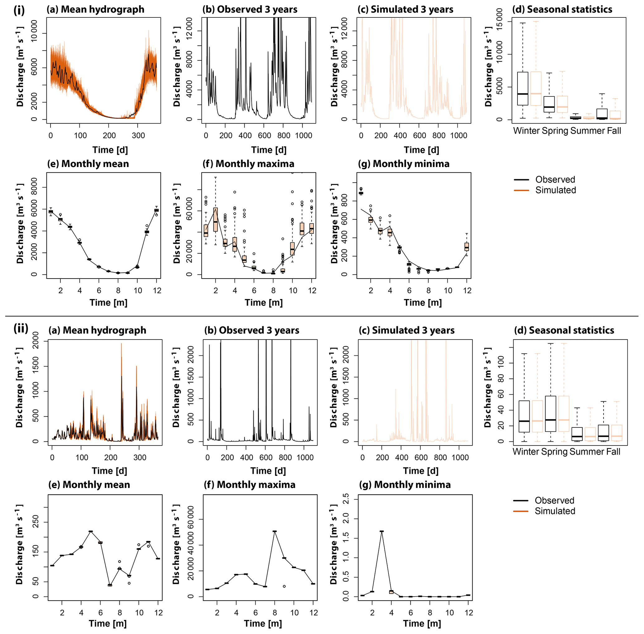
Figure 3 Comparison of observed (black) and simulated (orange) distributional discharge characteristics for (i) the station Nehalem River near Foss, OR (USGS 14301000, id 661) in the Pacific Northwest and (ii) the station Navidad River near Hallettsville, TX (USGS 08164300, id 464): (a) mean annual hydrographs, (b, c) observed and simulated time series for 3 years, (d) seasonal discharge distribution characteristics, (e) monthly mean discharge, (f) monthly maximum discharge, and (g) monthly minimum discharge.

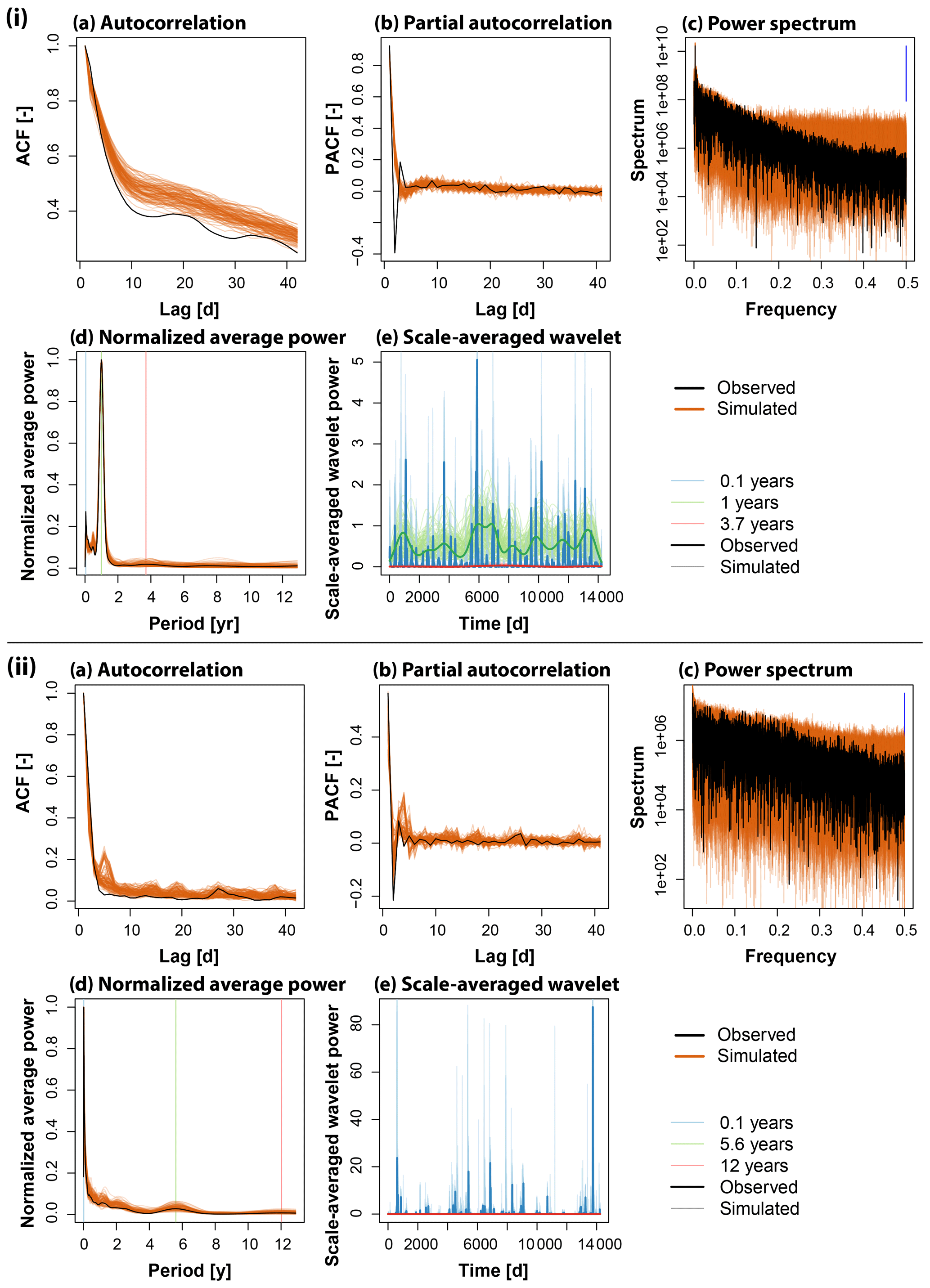
Figure 4 Comparison of observed (black) and simulated (orange) temporal discharge characteristics for (i) the station Nehalem River near Foss, OR (USGS 14301000, id 661) in the Pacific Northwest and (ii) the station Navidad River near Hallettsville, TX (USGS 08164300, id 464): (a) acf, (b) pacf, (c) power spectrum, (d) normalized average power, and (e) scale averaged-wavelet power.

Both high and low extremes are realistically modeled as illustrated by the boxplots depicting the distributions of the above and below threshold events of the four catchments in the Pacific Northwest (Fig. 5). While the median of the observed low- and high-flow distributions is well met by the simulated medians, again the simulations allow for the generation of extreme low and high flows going beyond the observed values because of the use of the theoretical kappa distribution.

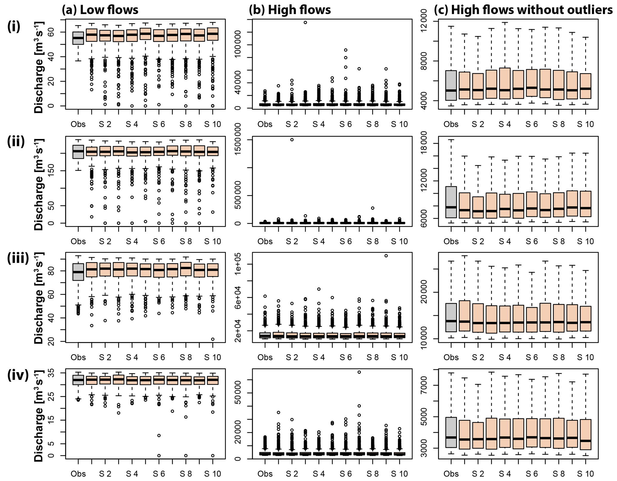
Figure 5 Comparison of observed (grey) (a) low- and (b, c) high-flow distributions (with and without outliers) with simulated distributions of 10 runs (orange) for the four catchments in the Pacific Northwest: (i) Calawah River near Forks, WA (USGS 12043000, id 590), (ii) Stillaguamish River near Arlington, WA (USGS 12167000, id 608), (iii) Nehalem River near Foss, OR (USGS 14301000, id 661), and (iv) Steamboat Creek near Glide, OR (USGS 14316700, id 668).

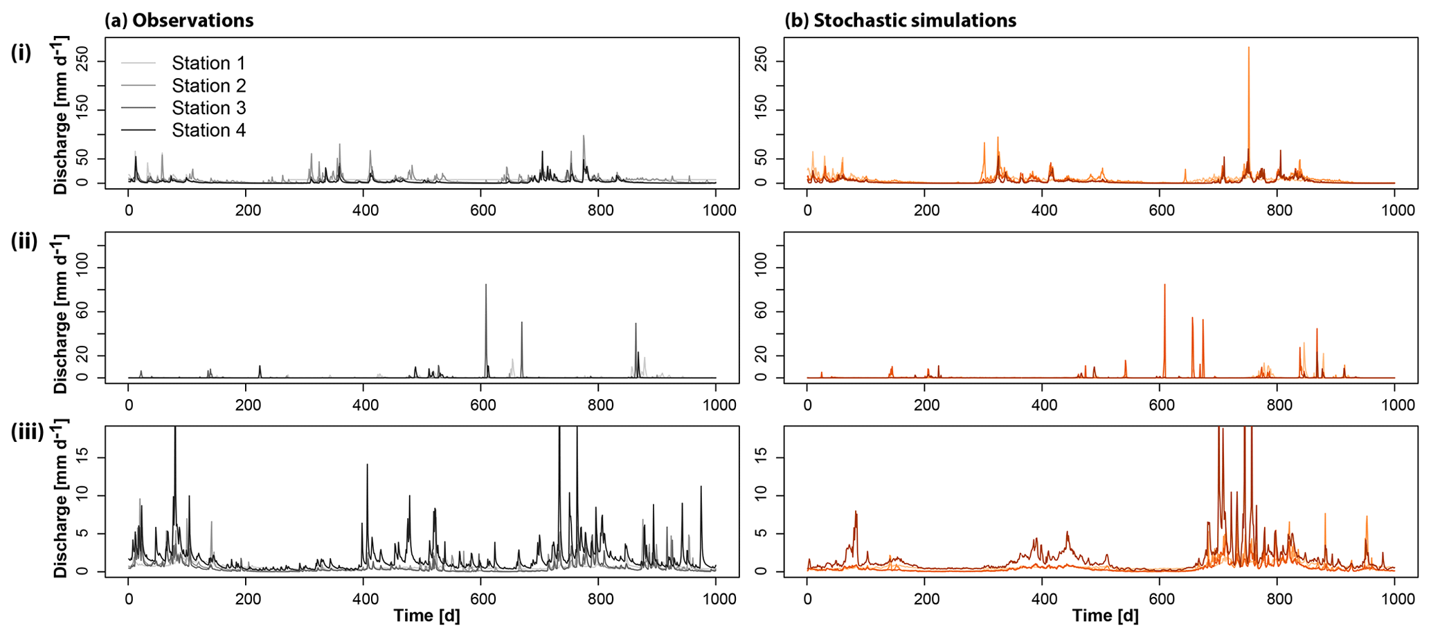
Figure 6 Comparison of 3 years of multi-site observations (a) with multi-site stochastic simulations (b) for the four catchments in the three example regions (i) Pacific Northwest, (ii) Texas, and (iii) Mid-Atlantic. Each region is displayed on its own scale.

4.2 Multi-site simulations

The stochastic simulation approach PRSim.wave not only allows for the reproduction of the distributional and temporal characteristics of time series at single sites, but also for the simulation of spatially coherent time series at multiple sites (Fig. 6). Independent of the region considered, the simulations realistically represent the observed behavior of the time series. This visual impression of a good performance with respect to the reproduction of spatial correlations in daily discharge data is confirmed by comparing observed and stochastically simulated cross-correlation functions for the catchments in the Pacific Northwest (Fig. 7). Both the shape and magnitude of the cross-correlation functions are well simulated. The good performance in terms of reproducing the general spatial dependence structure in the data can be generalized to other regions as shown by a comparison of observed and simulated variograms indicating a slight overestimation of spatial dependence for very long distances (>30^∘, ca. 3000 km; Fig. 8). Figures A1 and A2 demonstrate that neither the observed cross-correlation nor variogram would be captured by the simulations if the phases were randomized for each catchment individually instead of using the same set of randomized phases across all catchments. In the case of individual randomization, spatial dependence is not even captured for very short distances of a few kilometers.

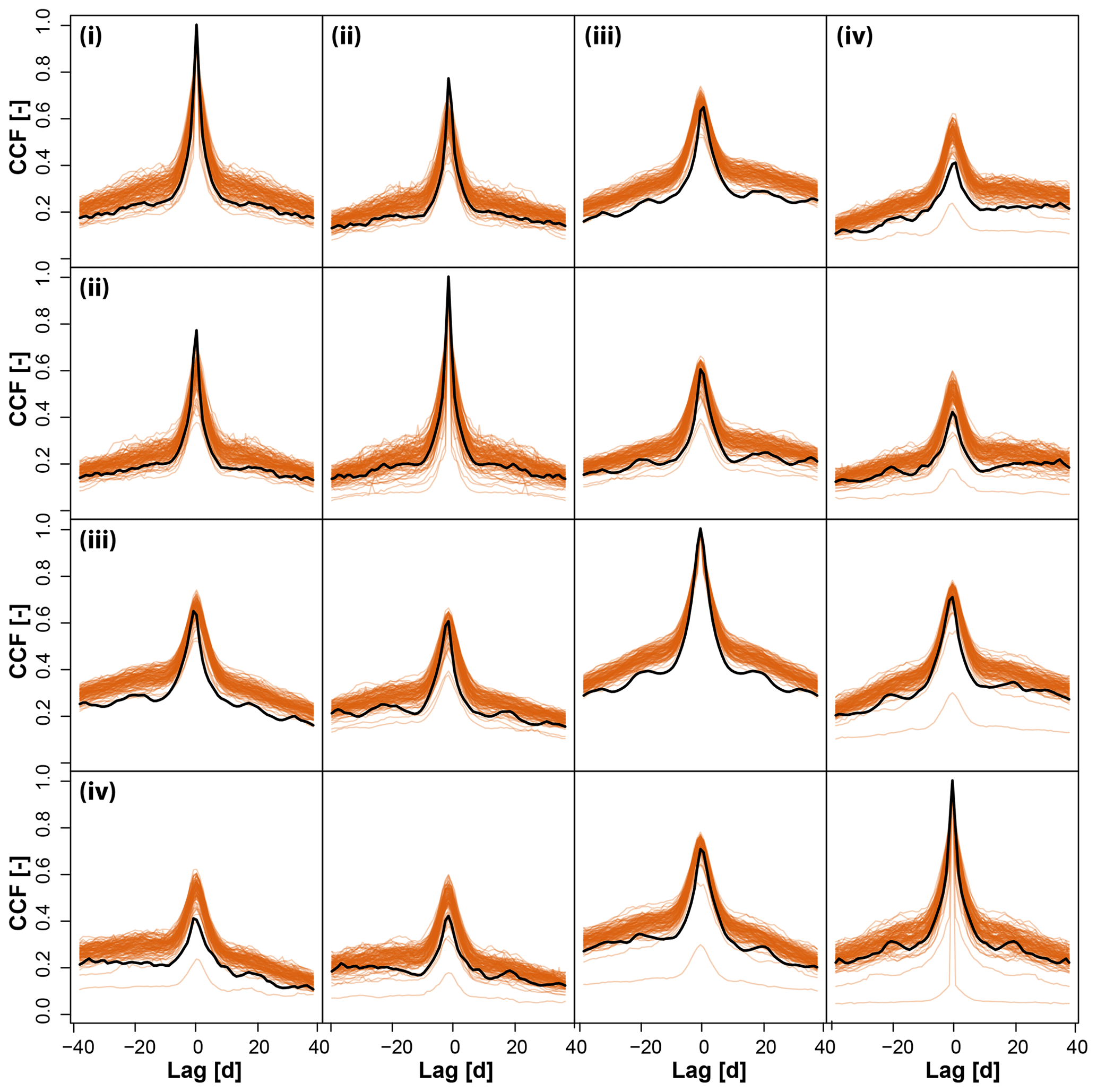
Figure 7 Comparison of observed (black) and simulated (orange) cross-correlation functions (ccfs) for the daily discharge values for pairs of stations in the set of four catchments (i–iv) in the Pacific Northwest.

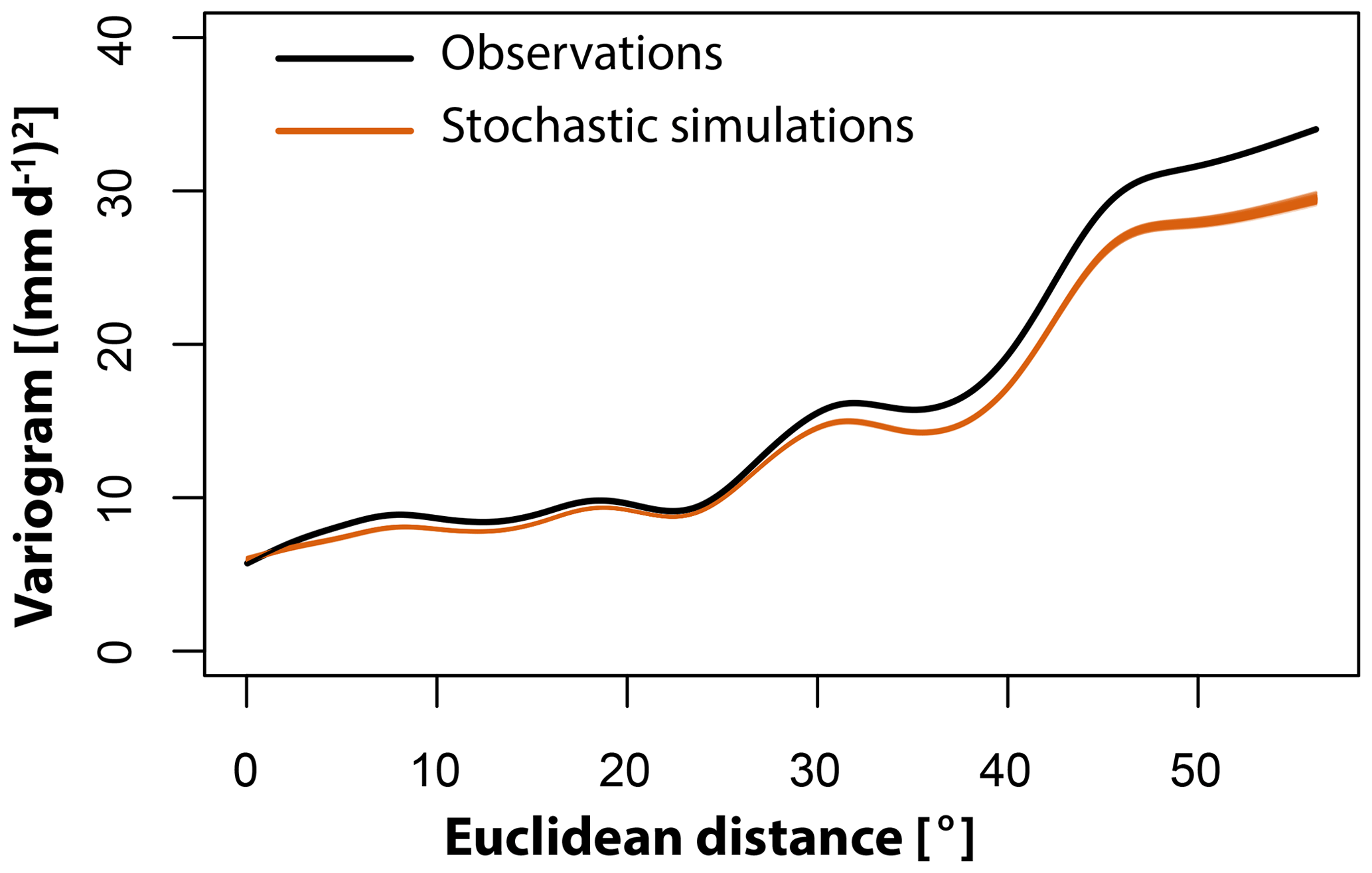
Figure 8 Comparison of observed variogram (black) with 100 variograms derived from the 100 simulation runs (orange).

Spatial dependencies are maintained not only for the bulk of the distribution, by which we mean the part of the distribution excluding extremes or outliers, but also for extreme values as illustrated by the peak-over-threshold (POT) values for the different stations in the three illustrated regions (Fig. 9). These results show that besides regional flood co-occurrences, the temporal clustering behavior of events is also reproduced.

Figure 9 Observed (a; black) vs. stochastically simulated (b; orange) POT events for the four stations (color shadings) in the three regions (i) Pacific Northeast, (ii) Texas, and (iii) Mid-Atlantic. Vertical bars indicate event occurrences over the 38 years.

The F-madograms shown in Fig. 10 indicate that there is generally good agreement between observed and simulated spatial dependence despite a slight overestimation of the spatial dependence of floods by the stochastic simulations. This overestimation means that a certain pair of stations may experience more joint floods according to the simulations than seen in the observations. The good agreement between observed and simulated spatial dependence and the weak overestimation in spatial dependence is also visible if we look at the tail dependence coefficient χ for the two thresholds 0.8 and 0.95 (Fig. 11). For most pairs of stations, both the simulations and observations indicate no tail dependence (grey dots). If the observations indicate tail dependence, the simulations mostly also simulate upper tail dependence (green dots). Only in very few cases do the simulations not capture the tail dependence in the observations (black dots). There are, however, quite a few cases where the simulations indicate tail dependence despite its absence in the observations (orange dots). Overall, the model shows good performance in the reproduction of observed spatial (in)dependencies.

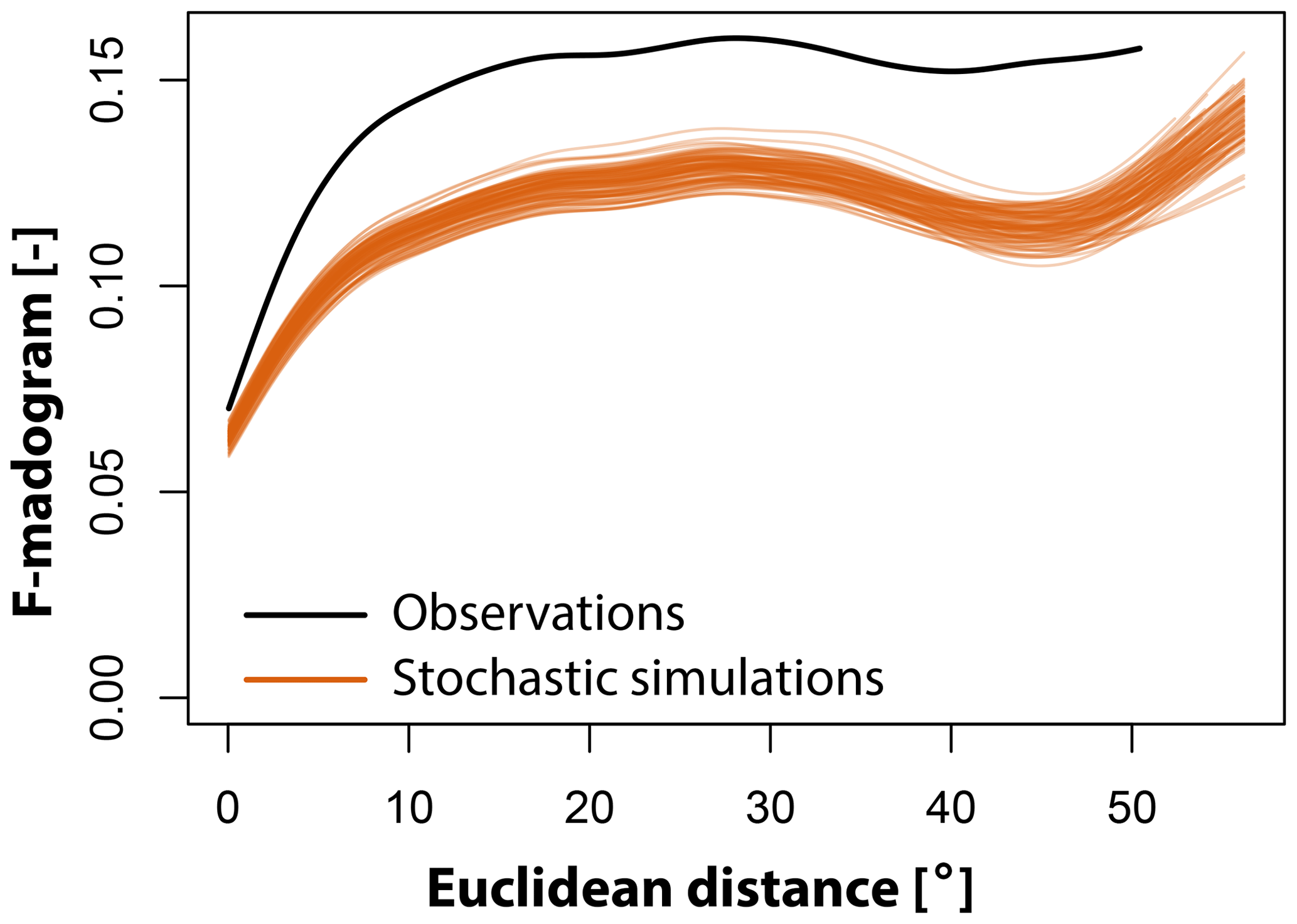
Figure 10 Observed (black) vs. simulated (orange) F-madograms, a measure of the strength of spatial dependence, plotted against Euclidean distance. The lower the value, the higher the dependence between a pair of stations.

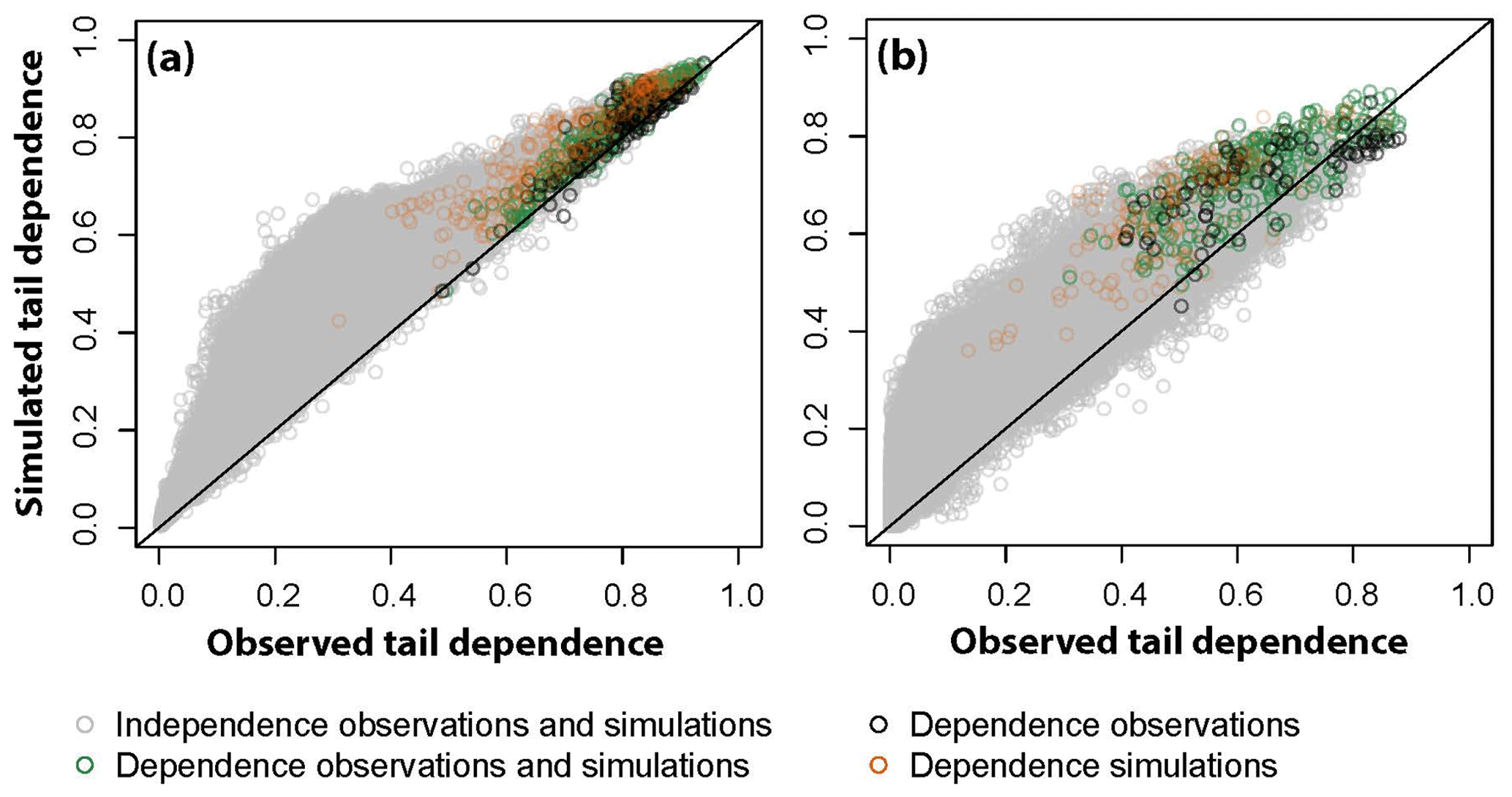
Figure 11 Observed vs. simulated tail dependence coefficient χ for the two thresholds 0.8 (a) and 0.95 (b). Grey dots indicate pairs of stations with no upper tail dependence, green dots pairs where both observations and simulations indicate upper tail dependence, black dots pairs of stations where only the observations indicate tail dependence, and orange dots pairs of stations where only the simulations indicate tail dependence.

5 Discussion

Similar to the Fourier transform based simulation approach PRSim by Brunner et al. (2019), the wavelet-based simulation approach PRSim.wave presented here allows for the generation of many time series of the same length as the observed series. This means that the representation of temporal dependence is limited to ranges within the length of the observed series. However, the modeled range of dependence is also limited to the one in the observed series if one very long time series is generated. In addition to the representation of temporal dependence, PRSim.wave allows for the reproduction of realistic spatial dependencies both in the general distribution and in extreme events. However, there is a slight tendency of the model to overestimate spatial dependence in extremes. A satisfactory representation of spatial dependence is not possible when using the Fourier transform as in PRSim. This difference between methods may be related to the fact that the wavelet transform compared to the Fourier transform does not necessitate a transformation to the normal domain and a back transformation to the domain of the skewed distribution, which has been shown to weaken spatial correlations (Embrechts et al., 2010; Papalexiou, 2018). A further improvement of the representation of cross-correlations and spatial dependencies may be achieved by using phase annealing, which modifies the phases in an iterative way in order to optimize certain statistics but increases the computational effort (Hörning and Bárdossy, 2018). The use of the kappa distribution in combination with the spatio-temporal model allows for the generation of extremes beyond the range of the observed values. However, it requires the fitting of many parameters, which make the model non-parsimonious (Koutsoyiannis, 2016). Depending on the application, the approach can therefore be used with a distribution with fewer parameters, a distribution fitted to a monthly instead of daily scale, or the empirical distribution.

The application of the approach is not limited to observed streamflow time series. It is applicable to other variables such as precipitation if combined with a suitable distribution as well as to modeled time series. The use of streamflow time series generated with a hydrological model extends the application of PRSim.wave to climate impact studies where a hydrological model is driven by meteorological time series generated with global and/or regional climate models. Potential future extensions also include the consideration of covariates to more explicitly model non-stationarities.

6 Conclusions

Our results show that the continuous, wavelet-based stochastic simulation approach PRSim.wave reliably simulates discharge and extremes at multiple sites. Thanks to a spatio-temporal model based on phase randomization, temporal short- and long-range dependencies, non-stationarities, and spatial dependencies are reproduced. In combination with the parametric kappa distribution, spatial extremes at multiple sites can be reliably simulated as well. The stochastic approach of PRSim.wave is very flexible and easy to use because of its availability in the R package PRSim. Its versatility and advantageous properties make it generally useful for various water management applications where spatio-temporal patterns are of interest and, in particular, valuable for hazard assessments requiring information on spatial extremes.

Appendix A: Simulations randomizing phases for each catchment individually

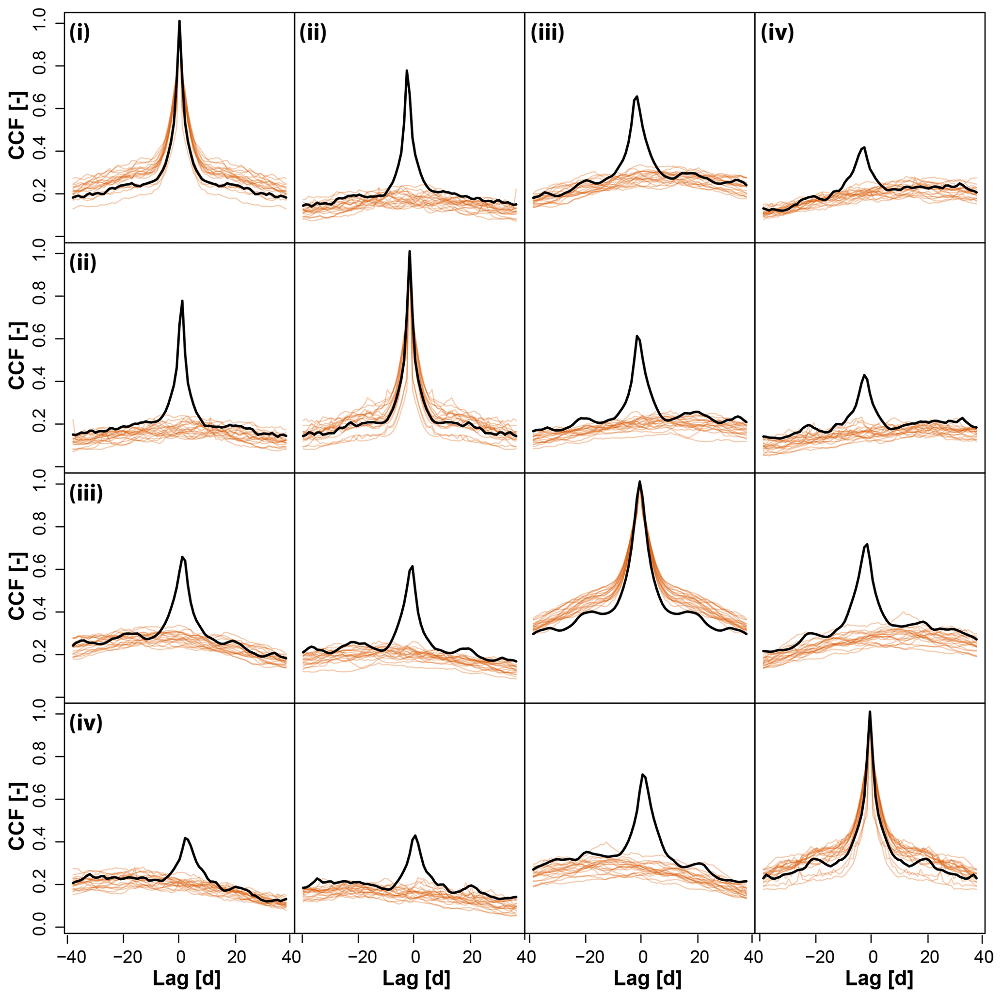
Figure A1 Comparison of observed (black) and simulated (orange) cross-correlation functions (ccfs) for the daily discharge values for pairs of stations in the set of four catchments (i–iv) in the Pacific Northwest. Twenty simulations were generated for each site individually, neglecting spatial dependence.

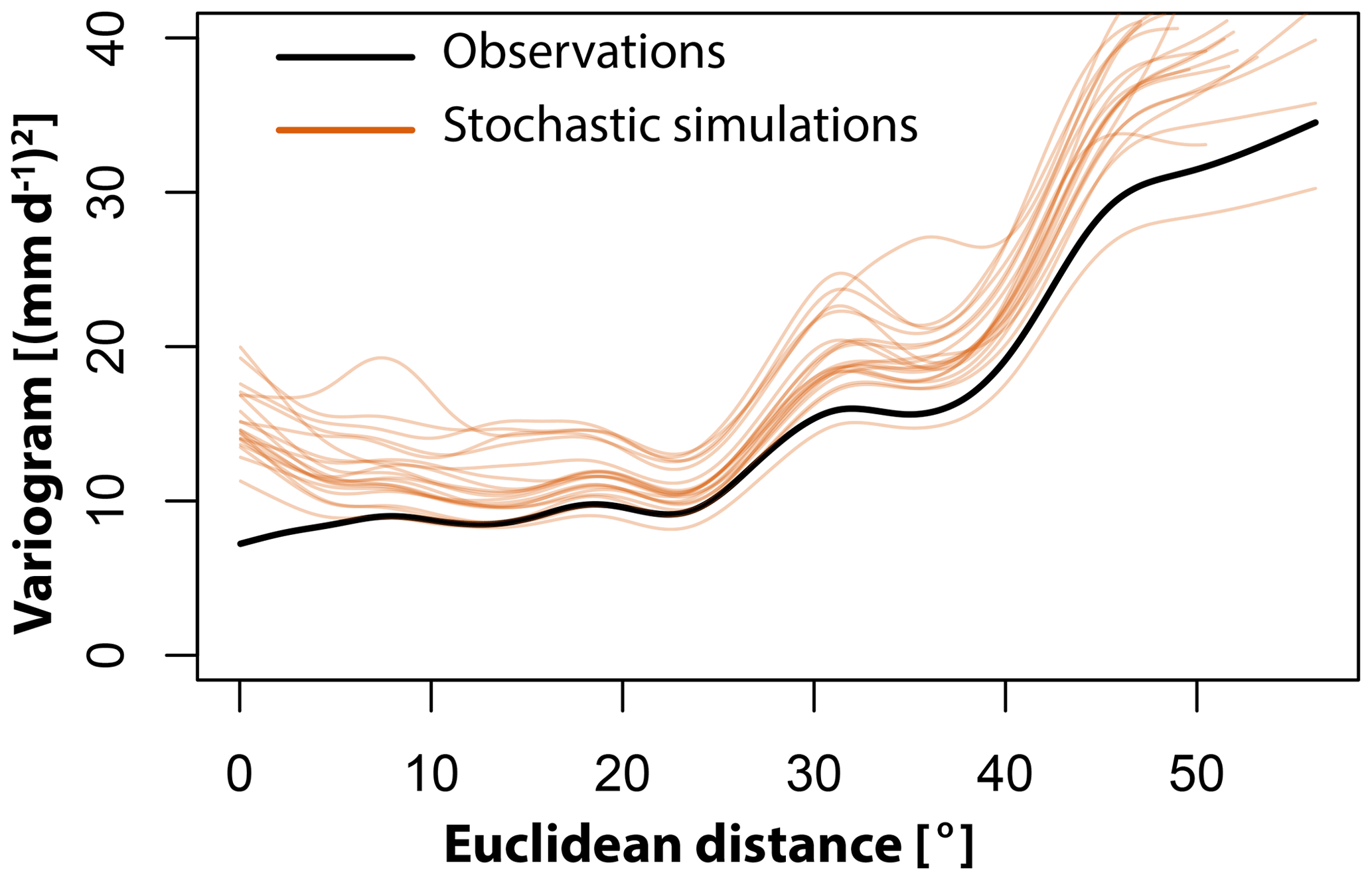
Figure A2 Comparison of observed (black) and simulated (orange) variograms for 20 simulation runs where the phases were randomized for each station individually.