the Creative Commons Attribution 4.0 License.
the Creative Commons Attribution 4.0 License.
 | 16 Jan 2020
A framework for deriving drought indicators from the Gravity Recovery and Climate Experiment (GRACE)
Helena Gerdener
Olga Engels
Jürgen Kusche
Identifying and quantifying drought in retrospective is a necessity for better understanding drought conditions and the propagation of drought through the hydrological cycle and eventually for developing forecast systems. Hydrological droughts refer to water deficits in surface and subsurface storage, and since these are difficult to monitor at larger scales, several studies have suggested exploiting total water storage data from the GRACE (Gravity Recovery and Climate Experiment) satellite gravity mission to analyze them. This has led to the development of GRACE-based drought indicators. However, it is unclear how the ubiquitous presence of climate-related or anthropogenic water storage trends found within GRACE analyses masks drought signals. Thus, this study aims to better understand how drought signals propagate through GRACE drought indicators in the presence of linear trends, constant accelerations, and GRACE-specific spatial noise. Synthetic data are constructed and existing indicators are modified to possibly improve drought detection. Our results indicate that while the choice of the indicator should be application-dependent, large differences in robustness can be observed. We found a modified, temporally accumulated version of the Zhao et al. (2017) indicator particularly robust under realistic simulations. We show that linear trends and constant accelerations seen in GRACE data tend to mask drought signals in indicators and that different spatial averaging methods required to suppress the spatially correlated GRACE noise affect the outcome. Finally, we identify and analyze two droughts in South Africa using real GRACE data and the modified indicators.
Please read the corrigendum first before continuing.
-
Notice on corrigendum
The requested paper has a corresponding corrigendum published. Please read the corrigendum first before downloading the article.
-
Article
(7535 KB)
-
The requested paper has a corresponding corrigendum published. Please read the corrigendum first before downloading the article.
- Article
(7535 KB) - Full-text XML
- Corrigendum
- BibTeX
- EndNote


Droughts are recurrent natural hazards that affect the environment and economy with potentially catastrophic consequences. Drought impacts range from reduced streamflow, water scarcity, and reduced water quality to increased wildfires, soil erosion, and increased quantities of dust, crop failure, and large-scale famine. With climate change and population growth, the frequency and impact of droughts are projected to increase for many regions of the world (IPCC, 2013). Drought types can be distinguished depending on their effect on the hydrological cycle (e.g., Changnon, 1987; Mishra and Singh, 2010). In this study we focus on hydrological drought, a multiscale problem which may last weeks or many years and which may affect local or continental regions. For example, the severe drought between mid-2011 and mid-2012 affected millions of people in the entire eastern Africa region (Somalia, Djibouti, Ethiopia, and Kenya) and led to famine with an estimated 258 000 deaths (Checchhi and Robinson, 2013). From 2012 to 2016, the US state of California experienced a historical drought that adversely affected groundwater levels, forests, crops, and fish populations and led to widespread land subsidence (Mann and Gleick, 2015; Moore et al., 2016). In contrast, European droughts, for example in 2018, typically last a few months in exceptionally dry summers. For South Africa, due to a complex rainfall regime, areas and the percentage of land surface affected by drought can vary strongly (Rouault and Richard, 2005).
Hydrological drought refers to a deficit of accessible water, i.e., water in natural and man-made surface reservoirs and subsurface storage, with respect to normal conditions. The propagation of drought through the hydrological cycle typically begins with a lack of precipitation, leading to runoff and soil moisture deficit, followed by decreasing streamflow and groundwater levels (Changnon, 1987). However, no unique standard procedures exist for measuring the deficit of each of these factors and for defining normal conditions. In order to arrive at operational definitions, which are required for triggering a response according to drought class for example, a large variety of drought indicators has been defined which typically seek to extract certain sub-signals from observable fields (Bachmair et al., 2016; Wilhite, 2016; Mishra and Singh, 2010; Van Loon, 2015). Reviews of hydrological drought indicators are contained in Keyantash and Dracup (2002), Wilhite (2016), Mishra and Singh (2010), and Tsakiris (2017). Streamflow is the most frequently used observable measurement in these studies.
Drought detection is mostly restricted to single fluxes (precipitation or streamflow) or storage (surface soil moisture or reservoir levels) that are easy to measure. Much fewer measurements are available to assess water content in deeper soil layers and groundwater storage deficit or the total of all storages. The NASA and German Aerospace Center (DLR) Gravity Recovery and Climate Experiment (GRACE) satellite mission, launched in 2002, has changed this situation since GRACE-derived monthly gravity field models can be converted to total water storage changes (TWSCs; Wahr et al., 1998). GRACE consisted of two spacecraft following each other, which were linked together by an ultra-precise microwave ranging instrument; these ranges are routinely processed to provide monthly gravity models and thus maps of mass change. Since other mass transports in the atmosphere and ocean are removed during the processing, GRACE indeed provides quantitative measure of surface and subsurface water storages (Chen et al., 2009; Frappart et al., 2013). Meanwhile, GRACE has been continued with the GRACE-FO (Follow-On) mission from which the first data are now available.
Studies of drought detection with GRACE-TWSC can be summarized in three groups: (i) using monthly maps of TWSC directly, (ii) partitioning TWSC time series into sub-signals that include drought signatures, or (iii) using indicators. For example, Seitz et al. (2008) investigated the 2003 heat wave over seven central European basins using GRACE time series; they found a good agreement between TWSC and the combination of net precipitation and evaporation. Other studies focused on drought detection using TWSC sub-signals, e.g., trends were used to identify drought in central Europe (Andersen et al., 2005) and for the region encompassing the Tigris, Euphrates, and western Iran (Voss et al., 2013). After decomposing GRACE-TWSC into a seasonal and non-seasonal signals, Chen et al. (2009) were able to detect the 2005 drought in the central Amazon river basin while, Zhang et al. (2015) identified two droughts in 2006 and 2011 in the Yangtze river basin. In the latter study, the El Niño–Southern Oscillation (ENSO) was identified as a possible driver for drought events in the Yangtze river basin. However, neither GRACE nor GRACE-FO enable one to separate different storage compartments, such as groundwater storage, without utilizing additional (e.g., compartment-specific) observations or model outputs, and their spatial and temporal resolutions (about 300 km and nominally 1 month respectively for GRACE) are limited. Several efforts are therefore focused on assimilating GRACE-TWSC maps into hydrological or land surface models (e.g., Zaitchik et al., 2008; Eicker et al., 2014; Girotto et al., 2016; Springer, 2019).
Thus, perhaps not surprisingly, a number of GRACE-based drought indicators have been suggested (e.g., Houborg et al., 2012; Thomas et al., 2014; Zhao et al., 2017), typically either based on normalization or percentile rank methods. However, a comprehensive comparison and assessment of these indicators is still missing, particularly in the presence of (1) trend signals as picked up by GRACE in many regions that may reflect non-stationary “normal” conditions, (2) correlated spatial noise that is related to the peculiar GRACE orbital pattern, and (3) the inevitable spatial averaging applied to GRACE, which results in smoothing out noise (Wahr et al., 1998). From a water balance perspective, GRACE-TWSC variability mainly represents monthly total precipitation anomalies (e.g., Chen et al., 2010; Frappart et al., 2013). It is thus obvious that GRACE drought indicators will contain signatures that are visible in meteorological drought indicators, yet the difference should explain the magnitude of other contributions (e.g., increased evapotranspiration due to radiation) to hydrological drought.
Figure 1 shows a time series of region-averaged, detrended and deseasoned GRACE water storage changes over eastern Brazil (Ceará state) compared to the region-averaged 6-month Standardized Precipitation Index (SPI) (McKee et al., 1993) to illustrate the potential of GRACE-TWSC for drought monitoring. As can be expected, TWSC and 6-month SPI appear moderately similar (correlation 0.43), characterized by positive peaks, for example at the beginning of 2004 and at the end of 2009, and negative peaks at the beginning of 2013. We also found correlations between TWSC and 6-month SPI in regions with different hydro-climatic conditions for the Missouri river basin (0.31), Maharashtra in western India (0.46), and South Africa (0.45) among other regions. This motivates us to modify common GRACE indicators to account for accumulation periods of input data, e.g., used with 6-month SPI but also for periods that are based on differences of input data. To our knowledge, this is the first study where (modified) indicators are tested in a synthetic framework based on a realistic signal that includes a hypothetical drought. We hypothesize that in this way we can (i) assess indicator robustness, with respect to identifying a “true” drought of given duration and magnitude, and (ii) understand how trend signals and spatial noise propagate into indicators and mask drought detection. In addition, we investigate to what extent the spatial averaging that is required for analyzing GRACE data affects indicators. For this, we compare spatially averaged gridded indicators to indicators derived from spatially averaged TWSC.
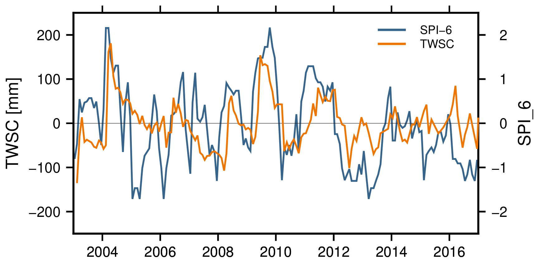
Figure 1Detrended and deseasoned GRACE-TWSC [mm] (orange) and the SPI [–] for 6 months of accumulated precipitation (blue), spatially averaged for Ceará, Brazil.
This contribution is organized as follows: in Sect. 2 we will review three GRACE-based drought indicators and modify them to accommodate either multi-month accumulation or differencing, while in Sect. 3 our framework for testing GRACE indicators in a realistic simulation environment will be explained. Then, Sect. 4 will provide simulation results and finally the results from real GRACE data. A discussion and conclusion will complete the paper.
Hydrological drought indicators are mostly based on observations of single water storages or fluxes, e.g., for precipitation, snowpack, streamflow, or groundwater. In general, indicator definitions can be arranged into four categories: (1) data normalization, (2) threshold-based, (3) quantile scores, and (4) probability-based (e.g., Zargar et al., 2011; Keyantash and Dracup, 2002; Tsakiris, 2017).
Since total water storage deficit may be viewed as a more comprehensive information source on drought, the advent of GRACE total water storage change data has led to new indicators being developed. For example, Frappart et al. (2013) developed a drought indicator based on yearly minima of water storage and a method for standardization, and Kusche et al. (2016) computed recurrence times of yearly minima through the generalized extreme value theory. Other indicators explore the monthly resolution of GRACE, e.g., the Total Storage Deficit Index (TSDI; Agboma et al., 2009), the GRACE-based Hydrological Drought Index (GHDI; Yi and Wen, 2016), the Drought Severity Index (DSI; Zhao et al., 2017), and the drought index (DI; Houborg et al., 2012). Further, Thomas et al. (2014) presented a water storage deficit approach to detect drought magnitude, duration, and severity based on GRACE-derived TWSC. To our knowledge, only the Zhao et al. (2017), Houborg et al. (2012), and Thomas et al. (2014) methods are able to detect drought events from monthly GRACE data without any additional information. Therefore, these three indicators will be discussed further.
In order to stress the link between GRACE-based and meteorological indicators, we first describe the relation of TWSC and precipitation. Assuming evapotranspiration (E) and runoff (Q) vary more regularly as compared to precipitation (i.e., ΔE=0 and ΔQ=0), the monthly GRACE-TWSC () corresponds to precipitation anomalies (ΔP) accumulated since the GRACE storage monitoring began.
where Δt is the time from t0 to t1. In contrast to Eq. (1), the difference between GRACE months as in
which corresponds to the precipitation anomaly accumulated between these months. Accumulated monthly TWSC thus corresponds to an iterative summation over the precipitation anomalies described by
In the following, we will discuss and extend the definition of Zhao et al. (2017), Houborg et al. (2012), and Thomas et al. (2014) GRACE-based indicators, which are hence referred to as the Zhao method, Houborg method, and Thomas method, respectively.
2.1 Zhao method
In the approach of Zhao et al. (2017), one considers GRACE-derived monthly gridded TWSC for n years as in
with
Let us define the monthly climatology, i.e., mean monthly TWSC, with j=1, …, 12 and the standard deviation of the anomalies in month j with respect to the climatological value as
Zhao et al. (2017) define their drought severity index (GRACE-DSI) as the standardized anomaly
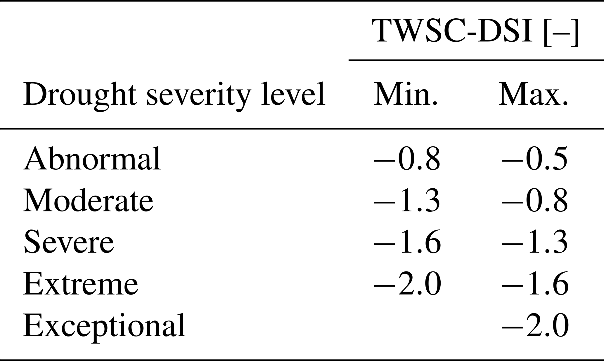
of a given month ti,j and provide a scale from −2.0 (exceptional drought) to +2.0 (exceptionally wet), as shown in Table 1. There is no particular probability distribution function (PDF) underlying the method; however if we assume the anomalies for a given month follow a Gaussian PDF, it is straightforward to compute the likelihood of a given month falling in one of the Zhao et al. (2017) severity classes. For example, 2.1 % of months would be expected to turn out to be a period of exceptional drought and 2.1 % as exceptionally wet. This can be applied to any other PDF.
Table 1Drought severity level of TWSC-DSI (Zhao et al., 2017). The values of TWSC-DSI are unitless.
Drought severity, however, should be related to the duration of a drought. For example McKee et al. (1993) showed how typical time scales of 3, 6, 12, 24, and 48 months of precipitation deficits are related to their impact on usable water sources. To account for the relation between severity and duration in the Zhao et al. (2017) approach, we consider q months accumulated of TWSC, which is approximately related to precipitation in Eq. (3) as
with for or equivalently written for q months of averaged TWSC as
For example for q=3, we would look for the 3-month running mean for December–January–February, January–February–March, and so on. In the next step, one computes, for example, the climatology and anomalies as with the original method. On the other hand, we can relate hydrological to meteorological indicators using Eq. (2). To develop a TWSC indicator that can be compared to indicators based on accumulated precipitation, one should rather consider the q-month differenced TWSC
Thus, as with TWSC-DSIi,j in Eq. (8), we can define two new multi-month indicators (TWSC-DSIA and TWSC-DSID) through standardization by using accumulated (A) and differenced (D) TWSC (Eqs. 9 and 11) as
and
Finally, it is obvious that sampling the full climatological range of dry and wet months is not yet possible with the limited GRACE data period. Therefore, Zhao et al. (2017) suggest applying a bias correction to avoid the under- or overestimation of drought events. This implies using TWSC from multi-decadal model runs, which is feasible but is not the focus of this study.
2.2 Houborg method
Houborg et al. (2012) define the drought indicator GRACE-DI via the percentile of a given month, ti,j, with respect to the cumulative distribution function (CDF). The GRACE-DI is applied to TWSC by
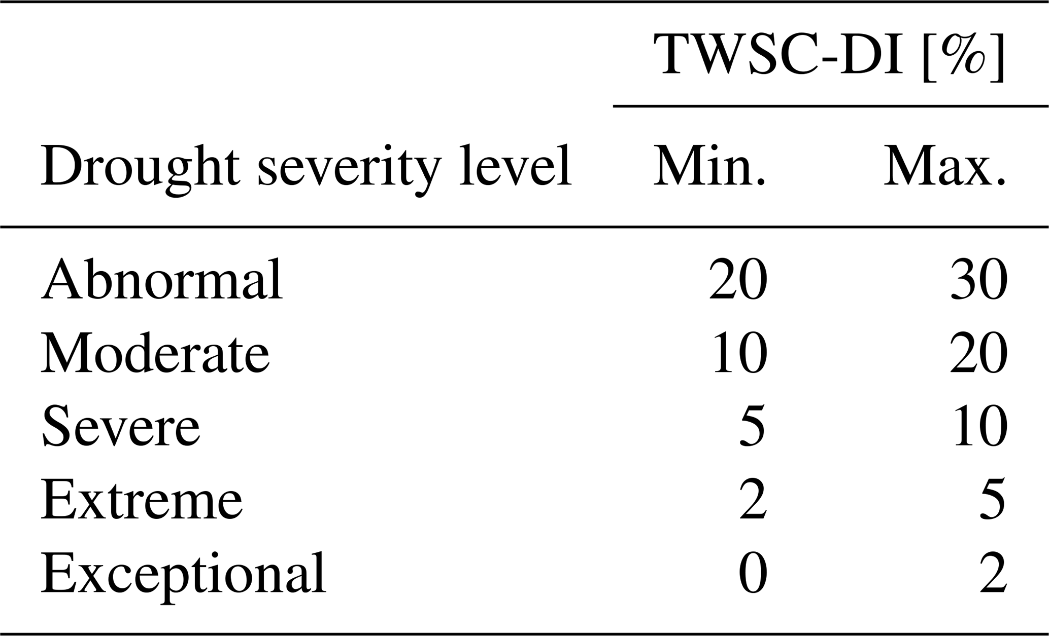
i.e., all years containing month j are counted for which TWSC is equal or lower than TWSC in month j and year i, and these are normalized by the number of years that contain month j. The indicator value is assigned to five severity classes as shown in Table 2. For example, exceptional droughts occur up to 2 % of the entire time period at any location.
Table 2Drought severity level of TWSC-DI (Houborg et al., 2012). The values of TWSC-DI are given in %.
Again, to relate drought severity to duration, we proceed via multi-month accumulation (Eq. 9) and differences (Eq. 11) resulting in the definition of two new indicators based on TWSC-DIi,j in Eq. (14),
Assuming again that the CDF equals the cumulative Gaussian PDF, 0.6 % of the months would be detected as exceptionally dry and 9.5 % of the months as abnormally dry. Houborg et al. (2012) applied the percentile approach separately to surface soil moisture, root zone soil moisture, and groundwater storage, which were derived by assimilating GRACE-derived TWSC into a hydrological model, and the CDFs were adjusted to a long-term model run. Here, we focus on a simulated TWSC environment for the GRACE period only, and, as explained in Sect. 2.1, we therefore disregard the bias correction.
2.3 Thomas method
Thomas et al. (2014) define a drought by considering the number of consecutive months below a threshold of TWSC. Given TWSC observations xi,j and a threshold c, we can compute anomalies by
While the threshold can be derived from different concepts, Thomas et al. (2014) use the monthly climatology xj (Eq. 6). Here, we also consider using a fitted signal for defining the threshold. The signal is computed by
with time t with a constant a0, a linear trend term a1, a constant acceleration term a2, annual signal terms b1 and b2, and similarly semi-annual signal terms c1 and c2. Trends and possible accelerations in GRACE-TWSC can result from many different hydrological processes. For example, accelerations can result from trends in the flux precipitation, evapotranspiration, and runoff (e.g., Eicker et al., 2016). In the following, the linear trends are denoted as trends, and constant accelerations are denoted as accelerations. The Thomas method then identifies drought events through the computation of their magnitude, duration, and severity: the magnitude or water storage deficit is equal to Δxi,j (Eq. 17), and the duration di,j is given by the number of consecutive months where TWSC is below the threshold. Thomas et al. (2014) propose a minimum number of 3 consecutive months required for the computation of drought duration. By using the deficit Δxi,j and the duration di,j, the severity si,j of the drought event can finally be computed by
Severity is therefore a measure of the combined impact of duration and magnitude of water storage deficit (see Thomas et al., 2014; Humphrey et al., 2016).
3.1 Methods
In order to analyze the performance of drought indicators, we first construct a synthetic time series of “true” total water storage changes on a grid. We base our drought simulations on the GRACE data model
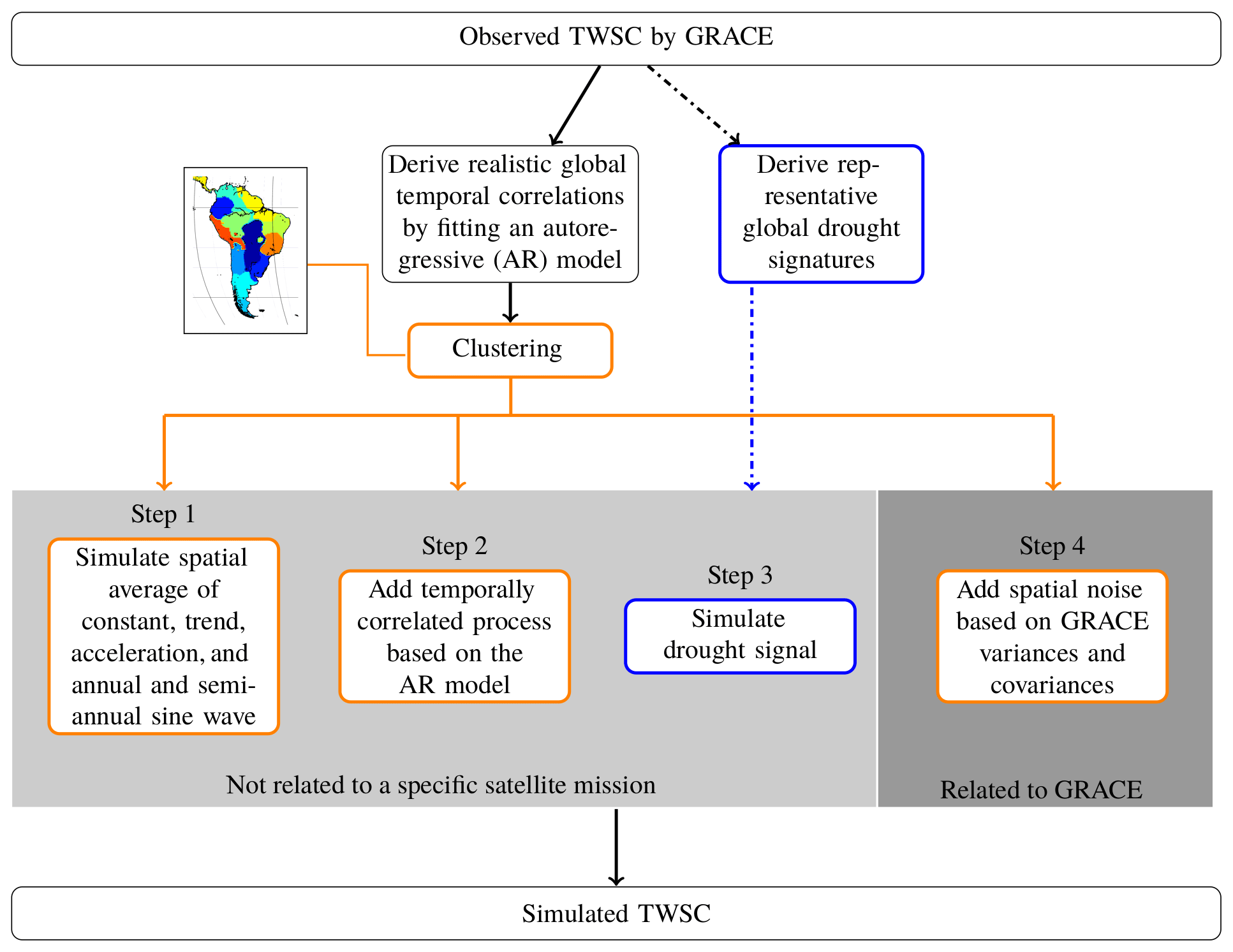
including the introduced (in Sect. 2.3) signal x (which contains seasonality and a constant, linear, and time-varying trend; Eq. 18), an interannual signal η (which has been detrended and deseasoned and which will carry the simulated true drought signature), and a GRACE-specific noise term ϵ. To simulate the true signal as realistically as possible using Eq. (20), we first analyze real GRACE-TWSC data following the steps summarized in Fig. 2. We derive (1) the signal components, constant, trend, acceleration, annual, and semi-annual sine wave, (2) temporal correlations, (3) a representative drought signal quantified by strength and duration, and (4) spatially correlated noise from GRACE error covariance matrices. While the first three steps are generic and can be used for simulating other observables, step 4 is directly related to the measurement noise (in this case the GRACE noise).
As an input to the simulation, GRACE-TWSC data are derived by mapping monthly ITSG-GRACE2016 gravity field solutions of degree and order 60, provided by the Graz University of Technology (Mayer-Gürr et al., 2016), to TWSC grids. As per standard practice, we add degree-1 spherical harmonic coefficients from Swenson et al. (2008) and degree 2, order 0 coefficients from laser ranging solutions (Cheng et al., 2011). Then, we remove the temporal mean field, apply DDK3 filtering (Kusche et al., 2009) to suppress excessive noise, and map coefficients to TWSC via spherical harmonic synthesis. We also remove the effect of ongoing glacial isostatic adjustment (GIA) following A et al. (2013).
Droughts are a multiscale phenomenon, and for a realistic simulation we must first define the largest spatial scale to which we will apply the model of Eq. (20). In other words, we first need to identify coherent regions in the input data for which our approach is then applied at the grid scale prior to step 1. For this, we apply two consecutive steps: we first compute temporal signal correlations by fitting an autoregressive (AR) model (Appendix A; Akaike, 1969) to detrended and deseasoned GRACE data. These TWSC residuals contain interannual and subseasonal signals including real drought information. Next, temporal correlation coefficients are used as an input for expectation maximization (EM) clustering (Dempster et al., 1977; Redner and Walker, 1984) because regions with similar residual TWSC correlation within the interannual and subseasonal signal are hypothesized here to be more likely affected by the same hydrological processes. The EM algorithm by Chen (2018) is modified to identify regional clusters. The EM algorithm alternates an expectation and a maximization step to maximize the likelihood of the data (e.g., Dempster et al., 1977; Redner and Walker, 1984; Alpaydin, 2009). More details about EM clustering are provided in Appendix B.
As a result of this procedure, we identified three clusters located in eastern Brazil (EB), southern Africa (SA), and western India (WI), which were indeed affected by droughts in the past (e.g., Parthasarathy et al., 1987; Rouault and Richard, 2003; Coelho et al., 2016). The location and shape of the three chosen clusters are shown in Fig. 3, and a global map of all clusters is provided in Fig. B1. Cluster delineations from the above procedure should not be confused with political boundaries or watersheds. The following simulation steps are then applied to each of these three clusters.
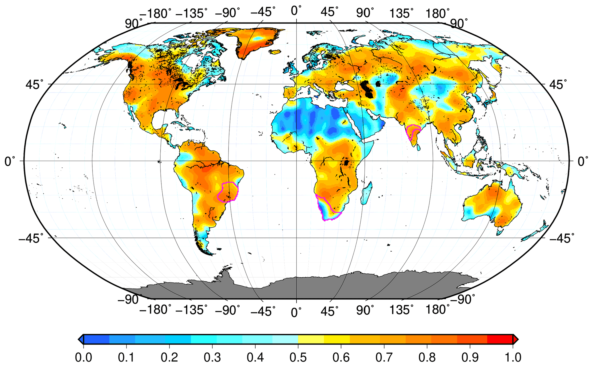
Figure 3AR(1) model coefficients (–) for global GRACE-TWSC. The polygons of the clusters of eastern Brazil, southern Africa, and western India are added in magenta.
In step 1 we estimate the signal coefficients according to Eq. (18) through least squares fit for each grid cell within the cluster. The coefficients are then spatially averaged to create a signal representative of the mean conditions within the region, and they are then used to create the constant, trends, and the seasonal parts of the synthetic time series. To simulate realistic temporal correlations at the regional scale (step 2), we use the AR model identified beforehand (Fig. 2) and again average AR model coefficients within the cluster. Then, we apply an AR model with the estimated optimal order and the averaged correlation coefficient (Eq. A1) to the synthetic time series to add temporal correlations.
Simulating realistic drought events in step 3 is challenging because, to our knowledge, no unique procedure to simulate realistic drought periods for TWSC exists. For this reason, we first perform a literature review to identify representative drought periods and magnitudes for selected regions. Among others, this includes the 2003 European drought and the drought in the Amazon basin in 2011 (e.g., Seitz et al., 2008; Espinoza et al., 2011, respectively). TWSC data within the identified drought period are then eliminated from the time series. In the next step, the parameters describing the constant, trend, acceleration, and seasonal signal components before and after the drought are used to “extrapolate” these signals during the drought period. By computing the difference of the original GRACE-TWSC time series and the continued signal in the drought period, we can separate non-seasonal variations from the data, which represent the drought magnitude. Our hypothesis is that the non-seasonal variations that we derive from the procedure possibly show a systematic behavior that can be parameterized. To extract this systematic behavior, all extracted droughts are transformed to a standard duration. To compare the different drought signals, a standard duration and a standard magnitude are arbitrarily set to 10 months and −100 mm, respectively. Finally, a synthetic drought signal η is generated by using the extracted knowledge of drought duration, drought magnitude, and systematic behavior, and it is added to the synthetically generated signal (Eq. 20).
In step 4 we add GRACE-specific spatially correlated and temporally varying noise ϵ (Eq. 20). First, for each month t we extract a full variance–covariance matrix Σ for the region grid cells from GRACE-TWSC. Then, whenever Σ is positive definite, we apply the Cholesky decomposition Σ=RTR, while if Σ is only positive semi-definite, we apply eigenvalue decomposition (Appendix C). Second, we generate a Gaussian noise series v of the length n, where n represents the number of grid cells within the cluster. Finally, spatial noise in month t is simulated through
The final synthetic signals for each grid cell within a cluster will thus exhibit the same constant, trend, acceleration, seasonal signal, temporal correlations, and drought signal, but it has spatially different and correlated noise. In the following, we will test the hypothesis that GRACE indicators depend on the presence of trend and random input signals using the generated synthetic time series.
We believe that our synthetic framework based on real GRACE data has multiple benefits: (i) we are able to identify the ability of an indicator by comparing the true drought duration and magnitude (step 3) to the indicator results; (ii) we are able to detect the influence of other typical GRACE signals on the drought detection; and (iii) the synthetic framework enables us to identify strengths and weaknesses of each analyzed indicator, and it thereby enables us to choose the most suitable indicator for a specific application.
3.2 Synthetic TWSC
Here, we will briefly discuss the TWSC simulation following methods described in the previous section.
When estimating AR models for detrended and deseasoned global GRACE data, we find that for more than 70 % of the global land TWSC grids are best represented by an AR(1) process (Fig. A1). Therefore, we apply the AR(1) model for each grid. Figure 3 shows the estimated AR model coefficients, which represent the temporal correlations, ranging from very low up to 0.3, e.g., over the Sahara or in southwestern Australia, up to about 0.8, e.g., in Brazil or in the southeastern US. EM clustering is then based on these coefficients.
The selected three clusters (Fig. 3) show differences between the signal coefficients of the functional model (step 1; Eq. 18), which are hence discussed for the linear trend. We find a mean linear trend for the eastern Brazil cluster of 1.0 mm TWSC per year, a higher trend of 5.0 mm per year in southern Africa, and for western India a trend of 56.3 mm per year (Table 3). The trends for eastern Brazil and southern Africa in GRACE-TWSC have been identified before (e.g., Humphrey et al., 2016; Rodell et al., 2018). We did not find confirmations for the strong linear trend in western India found, for example, by Humphrey et al. (2016), who identified about 7 mm per year within this region. We assume that in this study the linear trend for western India is estimated as strong positive because we additionally identify a strong negative acceleration of −8.03 mm yr−2 in western India. However, our simulation will cover weak and strong trends. In fact, all coefficients show strong differences, which suggests that we cover different hydrological conditions when simulating TWSC for the three regions. In step 2 we identify correlations of 0.74 in eastern Brazil, 0.79 in western India, and 0.42 in southern Africa (Table 3).
Table 3Coefficients (a0 to c2 from Eq. 18 and ϕ1 from Eq. A1) for signals contained in GRACE-TWSC that were extracted within the clusters of eastern Brazil, southern Africa, and western India. These coefficients are used to simulate synthetic TWSC.

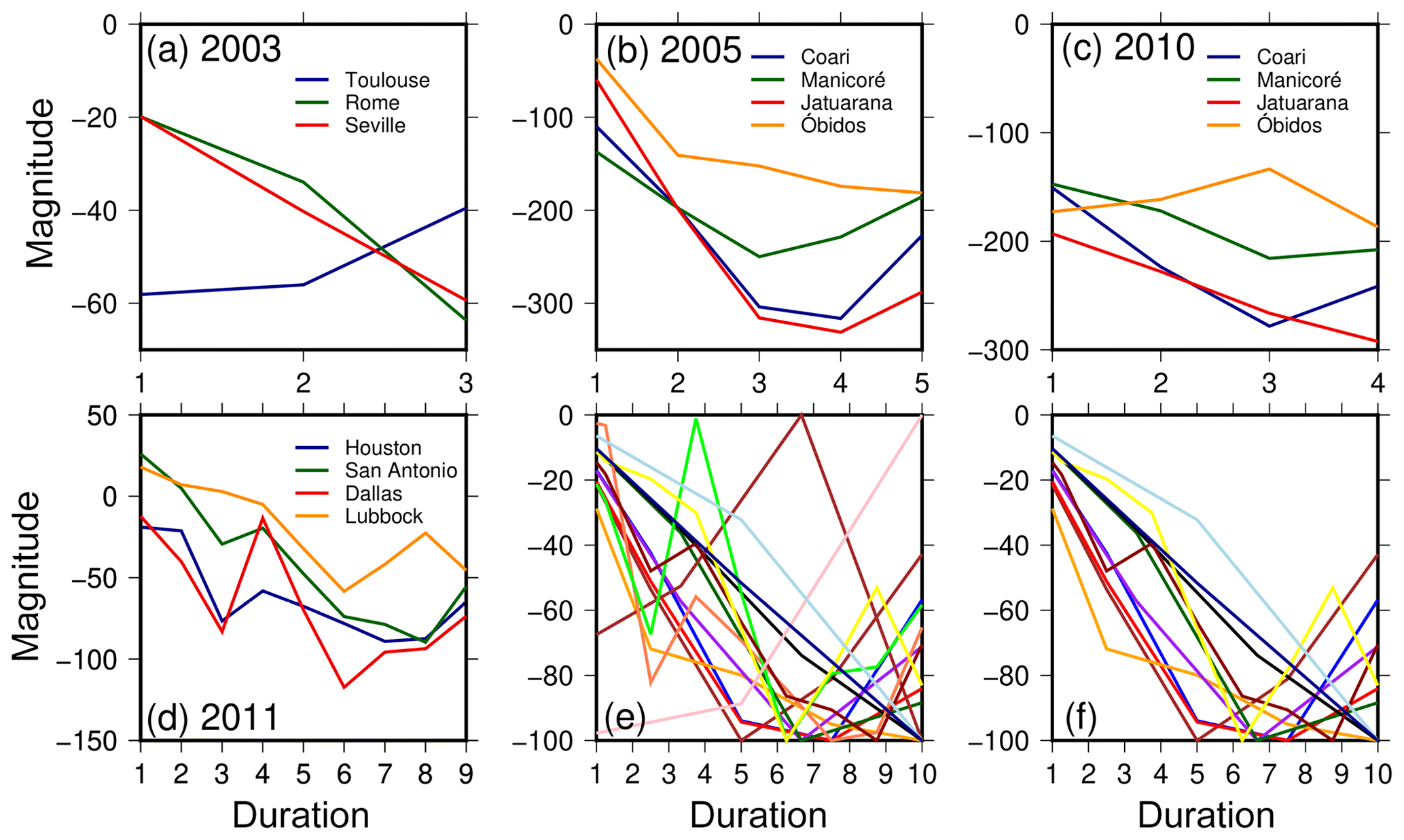
Figure 4Extracted drought periods from GRACE-TWSC for the droughts in (a) Europe in 2003, (b) the Amazon river basin in 2005, (c) the Amazon river basin in 2010, and (d) Texas in 2011. (e) All droughts from (a)–(d) were transformed to standard severity and duration. Panel (f) is the same as (e) but after removing four time series with significant temporally different behavior.
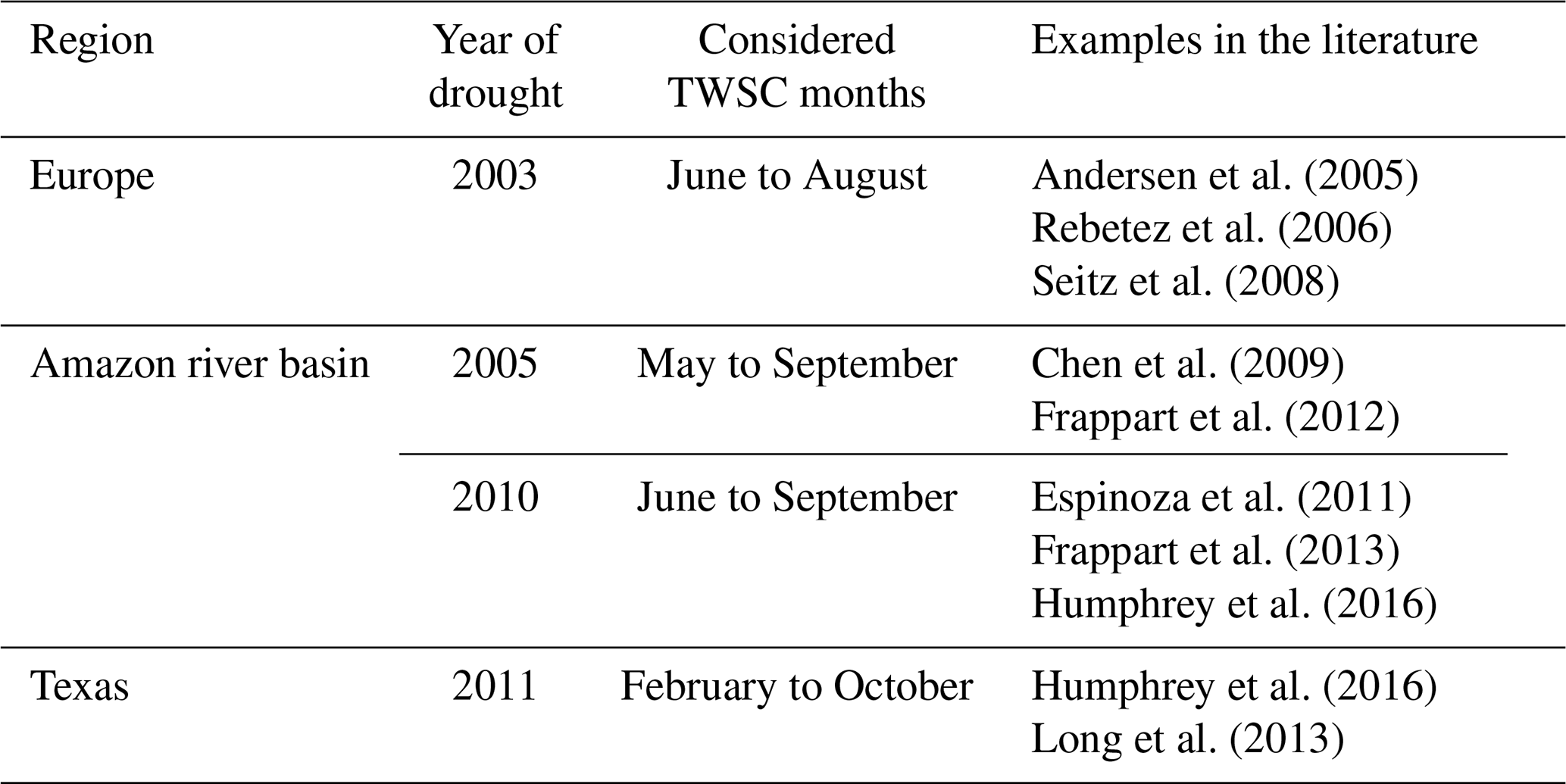
Performing literature research for drought duration and magnitude (step 3) led to four droughts seen in GRACE-TWSC (Table 4): the 2005 and 2010 droughts in the Amazon (e.g., Chen et al., 2009; Espinoza et al., 2011), the 2011 drought in Texas (e.g., Long et al., 2013), and the 2003 drought in Europe (e.g., Seitz et al., 2008). To extract the drought duration, we compared drought onset and end identified in these and other papers. We found that different studies do not exactly match, with inconsistencies likely due to different methodologies used. Furthermore, some authors only specified the year of drought. Droughts extracted from the literature had a duration of 3 to 10 months (Fig. 4a–d). Unless otherwise specified, we decided to base our simulations on a duration of 9 months to represent a clear identifiable drought duration. Extracted drought magnitudes range from about −20 to −350 mm TWSC (Fig. 4a–d). Therefore, in order to simulate a drought magnitude that has a clear influence on the synthetic time series, we set the magnitude to −100 mm.
Andersen et al. (2005)Rebetez et al. (2006)Seitz et al. (2008)Chen et al. (2009)Frappart et al. (2012)Espinoza et al. (2011)Frappart et al. (2013)Humphrey et al. (2016)Humphrey et al. (2016)Long et al. (2013)Table 4Drought events in Europe, the Amazon river basin, and Texas with corresponding duration taken from the literature.
As described in Sect. 3.1, we transform these water storage droughts to a standard duration and magnitude to understand whether a typical signature can be seen. However, Fig. 4e remains inconclusive as there are, in particular, four standardized droughts, which show a very different temporal behavior: Toulouse in 2003, Óbidos in 2010, and Houston and Dallas in 2011. When we remove those four time series (Fig. 4f), a systematic behavior can be identified and parameterized using a linear or quadratic temporal model. However, due to these difficulties, we decided to use the most simple TWSC drought model, i.e., a constant water storage deficit within a given time span.

Figure 5Synthetic TWSC (mm) without (light blue) and with spatial GRACE noise (dark blue) using average parameters for the clusters in eastern Brazil (EB), southern Africa (SA), and western India (WI). Light brown shows the simulated drought period.
In step 4, we project the simulation on a 0.5∘ grid and add spatially correlated GRACE noise. A few representative time series of the gridded synthetic total water storage change are shown in Fig. 5 for eastern Brazil, southern Africa, and western India for the GRACE time period from January 2003 to December 2016. The effect of realistic GRACE noise (dark blue vs. light blue) is clearly visible, particularly for the SA case with low annual amplitude. The synthetic drought period is placed from January to September 2005 (light brown) in all three regions. Synthetic TWSC variability includes considerable (semi-)annual variations for EB based on Table 3. Furthermore, a strong negative acceleration is contained in the synthesized time series for eastern Brazil (Table 3) leading to strong negative TWSC towards the end of the time series. For western India a strong positive trend leads to low TWSC at the begin of the time series.
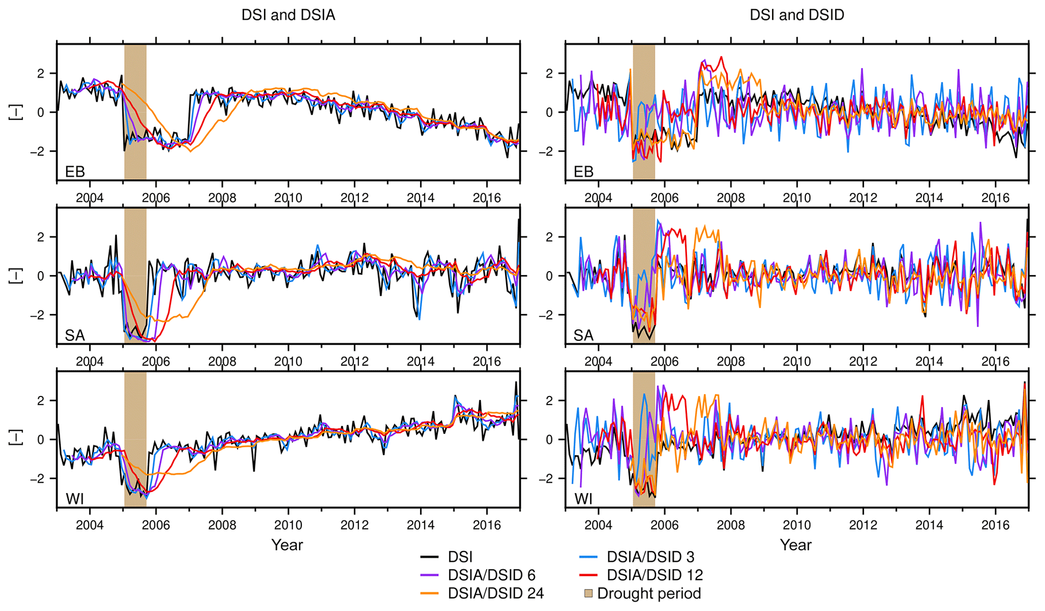
Figure 6A representative example of the synthetic DSI, DSIA, and DSID (–) for the eastern Brazil (EB), southern Africa (SA), and western India (WI) cluster over the periods of 3, 6, 12, and 24 months. Light brown shows the synthetic constructed drought period.
4.1 Synthetic TWSC: masking effect of trend and seasonality
Here, we analyze how non-drought signals, such as a linear or accelerated water storage trend and the ubiquitous seasonal signal, propagate through the Zhao, Houborg, and Thomas GRACE indicators (Sect. 2) and potentially mask a drought. To this end, we select representative time series from each of the three synthetic grids of total water storage changes for eastern Brazil, southern Africa, and western India and apply the three methods. Since all results are based on TWSC, we refer to TWSC-DSIA, TWSC-DSID, TWSC-DIA, and TWSC-DID as DSIA, DSID, DIA, and DID, respectively (again, with accumulated (A) and differenced (D) variants).
We first assess the temporal characteristics of the Zhao method (Sect. 2.1). Figure 6 (left) shows time series for the DSI and DSIA (with 3, 6, 12, or 24 months of accumulated TWSC). It is obvious that trend and acceleration propagate into both DSI and DSIA (see eastern Brazil and western India). Resulting indicator values (e.g., for the years 2015 and 2016) are lower than those compared to a small trend (southern Africa) and this may lead to misinterpretations because a severe-to-mild drought is identified (−2 to −0.5), while none is actually simulated. In contrast, the actual simulated drought in 2005 is only identified as a moderate drought (values up to −1.0) for EB.
In the presence of a small trend (5.0 mm yr−1) and acceleration (−0.38 mm yr−2; Table 3, SA), we do identify an exceptional drought (Fig. 6 DSIA for southern Africa). This shows that the drought strength that we chose does indeed lead to a correct identification of exceptional drought if no masking occurs (but in the presence of GRACE noise), so at this point we can determine that exceptional drought represents the true drought severity class. As expected, a trend and/or an acceleration signal that are frequently observed in GRACE analyses can lead to misinterpretations in the indicators. However, the influence of the trend or acceleration also depends on the timing of the drought period within the analysis window. For example, assuming we simulate the time series with the same trend or acceleration but the drought were to occur in 2014, the drought detection would not have been influenced as much. Therefore, we decided to set up an additional experiment and discuss the influence of different trend strengths for the drought detection (Sect. 4.3).
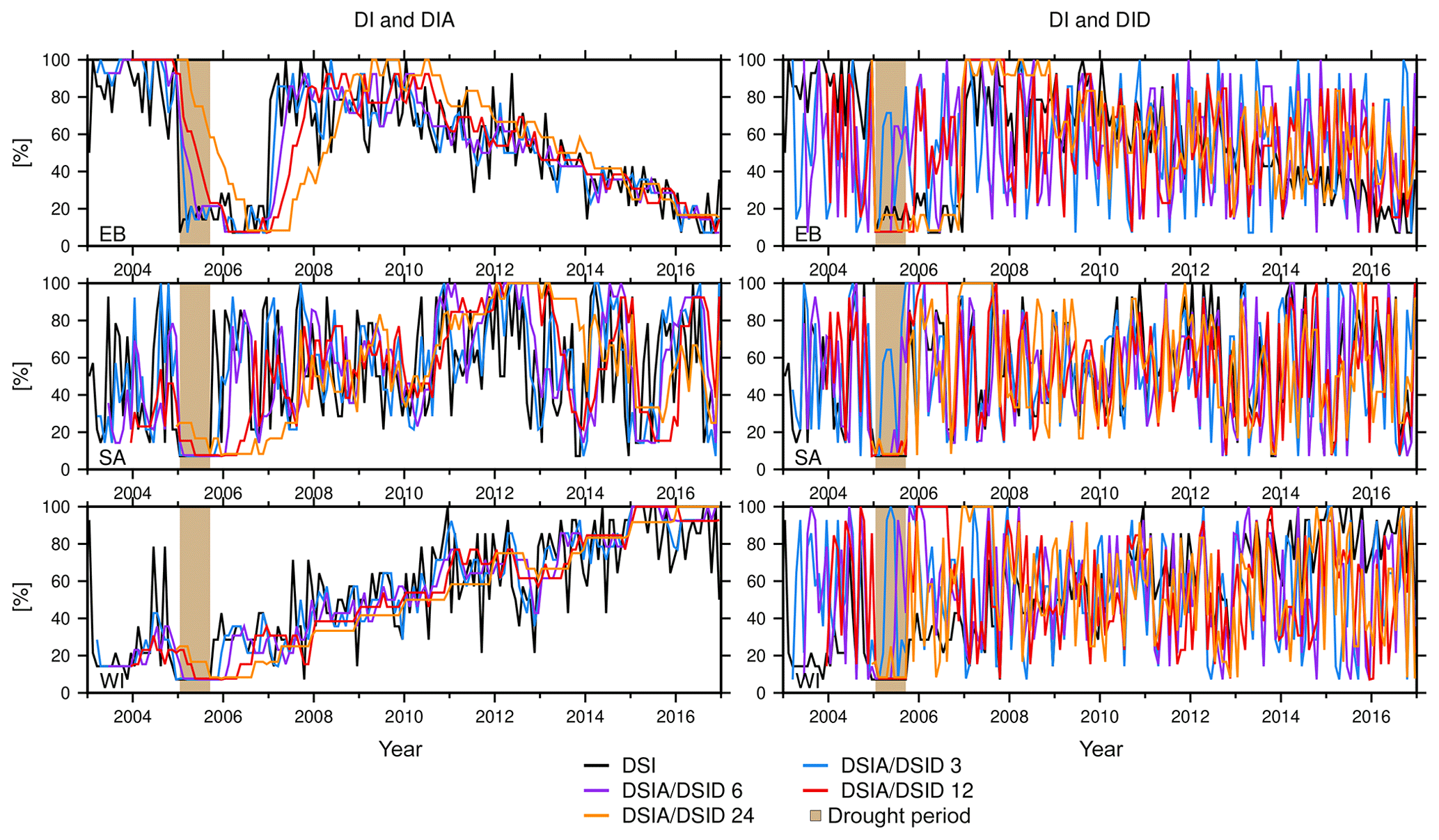
Figure 7A representative example of the synthetic DI, DIA, and DID (%) for the eastern Brazil (EB), southern Africa (SA), and western India (WI) cluster over the periods of 3, 6, 12, and 24 months. Light brown shows the synthetic constructed drought period.
The analysis reveals that DSI and DSIA indicators are sensitive with respect to trends, while they are less sensitive to the annual and semi-annual signal. The seasonal signal is clearly dampened (e.g., compare Fig. 5 to the DSIA in Fig. 6). This is caused by removing the climatology within the Zhao method (Eq. 8). Comparing DSIA3, DSIA6, DSIA12, and DSIA24, e.g., for eastern Brazil, suggests that with a longer accumulation period, indicator time series are increasingly smoothed, and less severe droughts are identified (Fig. 6, left). Furthermore, the drought period appears shifted in time, and its duration is prolonged. This can lead to missing a drought identification if a trend or an acceleration is contained in the analyzed time series, for example for the 24-month DSIA for eastern Brazil. We find that all DSIA data are able to unambiguously detect a drought close to 2005, assuming that neither trend nor acceleration is apparent (Fig. 6 DSIA for southern Africa). Particularly, the 3- and 6-month DSIA data identify the drought close to 2005 for southern Africa, and its computation appears to dampen the temporal noise that is present in the DSI.
In contrast we find that the 3-, 6-, 12-, and 24-month TWSC-differencing DSID data exhibit stronger temporal noise as compared to the DSIA and the DSI. This can be seen in the light of Eq. (2) – these indicators are closer to meteorological indicators and thus do not inherit the integrating property of TWSC. The DSID does not propagate a trend and acceleration, annual signal, or semi-annual signal. All DSID time series, for example for eastern Brazil (Fig. 6, right), show a strong negative peak within the drought period, but this peak does not cover the entire drought period for the 3-, and 6-month differenced DSID. The negative peak within the drought period is always followed by a strong positive peak; when we consider Eq. (2), this lends to the interpretation that a pronounced drought period is normally followed by a very wet event to return to “normal” water storage condition. Despite higher noise and the positive peak and contrary to the DSIA, all DSID data (DSID3, DSID6, DSID12, and DSID24) correctly identify the drought within 2005 to be exceptionally dry for eastern Brazil and southern Africa. All different DSID time series for WI identify at least a moderate drought.
Analysis of the Houborg method shows a broadly similar behavior as compared to the Zhao method: the sensitivity of drought detection to an included trend or acceleration depends on the indicator type. Using the DIA we can confirm the large influence of the trend or acceleration on the indicator value, which is not the case for DID (e.g., Fig. 7 DIA and DID for eastern Brazil). Annual and semi-annual water storage signals are all considerably weakened in the Houborg method because they are effectively removed when computing the empirical distribution for each month of the year. Differences to the Zhao method appear when comparing more general properties; e.g., we find that DI is more noisy and the range of output values is restricted to about 7 % to 100 % (Fig. 7). This restriction is caused by the length of the time series; e.g., assuming we strive to identify an event with exceptional dry values (≤2 %), we would need at least 50 years of monthly observations. Yet, with GRACE we only have about 14 years of good monthly observations, so the simulation was also restricted to this period. If we then take the driest value that might occur only once, we can compute the minimum value of DI to be 7.14 %. Hence the detection of a period of exceptional or extreme drought is not possible when referring to the duration of the GRACE-TWSC time series. As mentioned in Sect. 2.2, Houborg et al. (2012) applied a bias correction to the empirical CDF to mitigate this restriction. We do not follow Houborg's approach here in order to focus on the synthetic environment instead of the availability of model outputs.
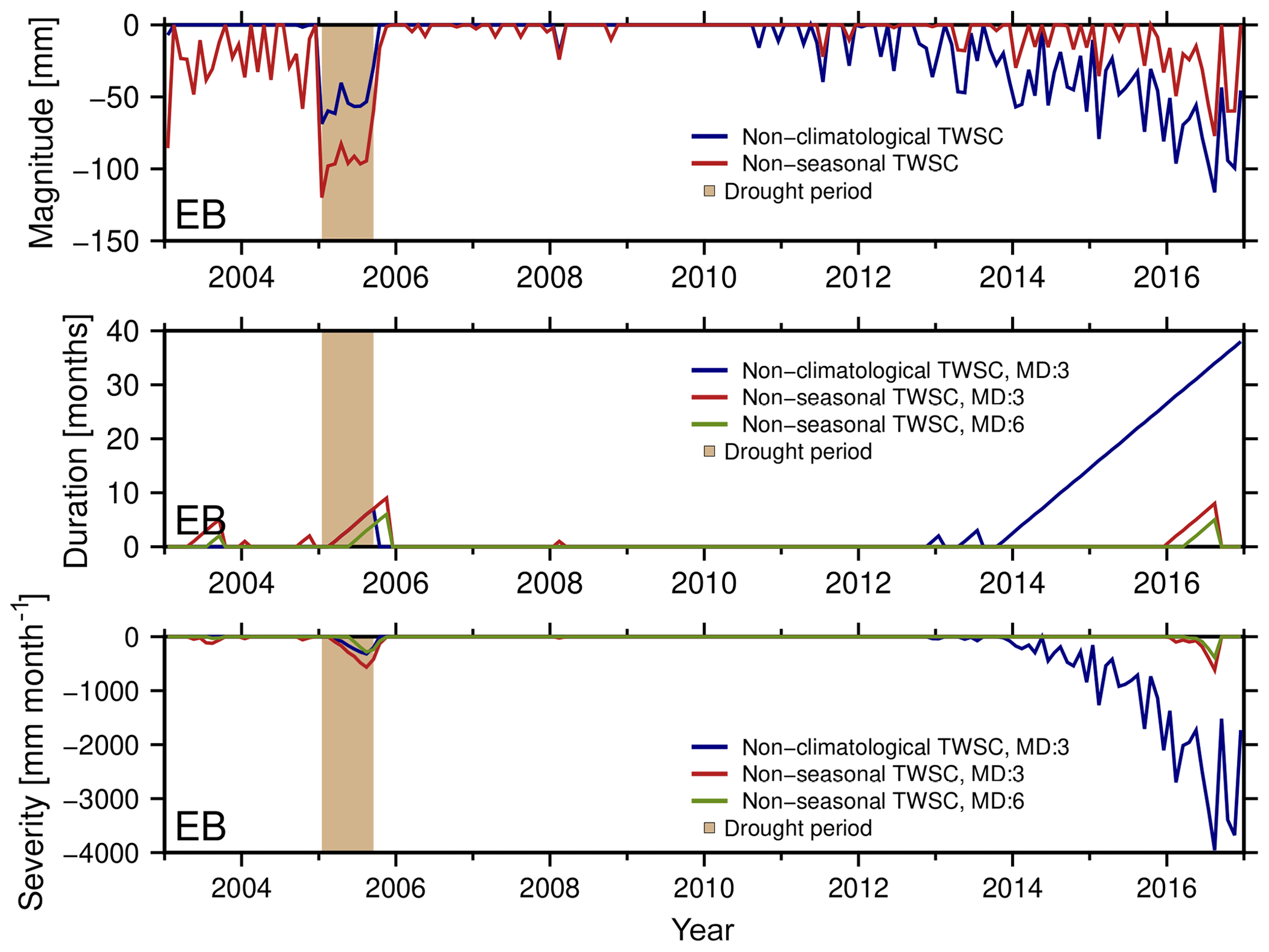
Figure 8Drought magnitude (mm), duration (months) and severity (mm month−1) for the cluster in eastern Brazil (EB) using TWSC with the removed climatology (dark blue) and TWSC with removed trend and seasonal signal (red). The minimum duration (MD) is set to 3 months (blue and red) or 6 months (green). Light brown shows the synthetic constructed drought period.
The Thomas method is applied to simulated TWSC data to derive the magnitude, duration, and severity of a drought, which we show in Fig. 8 for the EB region. We find that the linear trend and acceleration propagate into the magnitude (Fig. 8, top) when using TWSC deficits with climatology removed (blue, Eq. 6) compared to using TWSC deficits with removed trends, accelerations, and seasonality (red, Eq. 18). When using non-climatological TWSC (blue), we identify a strong deficit in 2015 and 2016 (Fig. 8, top), which suggests a duration of up to 38 months (Fig. 8, center) and a severity of about −4000 mm months (Fig. 8, bottom). Using the detrended and deseasoned TWSC (red), drought is mainly detected in the true drought period (2005) and not at the end of the time series. Thus we conclude that a trend or acceleration indeed modifies the drought detection.
Results so far were derived by imposing a minimum duration of 3 months (blue and red). When moving to a minimum duration of 6 consecutive months (green, Fig. 8, middle and bottom) we find this would lead to a decrease in identified severity by half, and the beginning of the drought period shifts 3 months in time. This is in line with Thomas et al. (2014). The same findings are made for southern Africa and western India.
4.2 Synthetic TWSC: effect of spatially correlated GRACE errors
Here, we investigate how robust the Zhao, Houborg, and Thomas indicators are with respect to the spatially correlated and time-variable GRACE errors. However, any analysis must take into account that GRACE results cannot be evaluated directly at grid resolution.
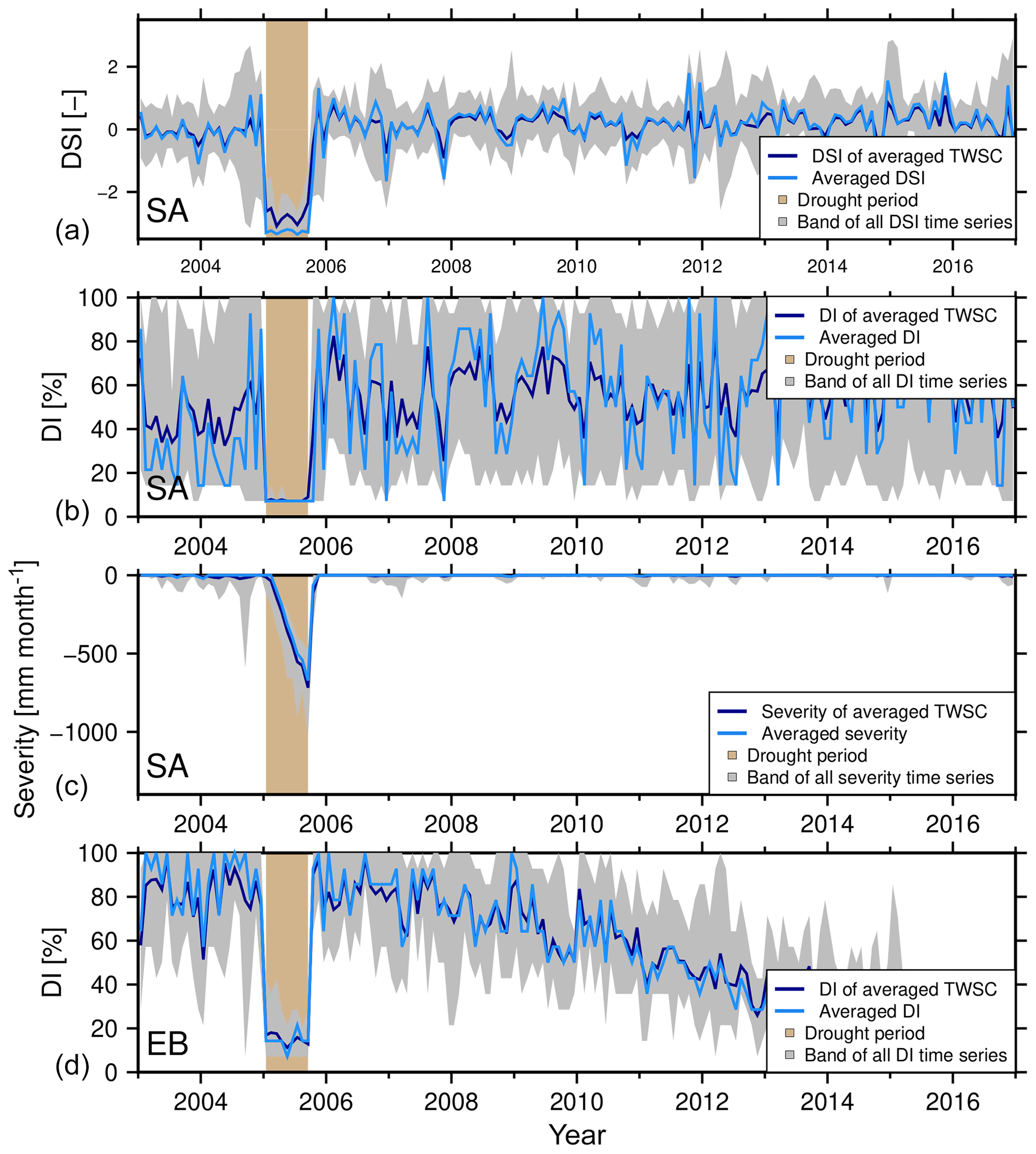
Figure 9DSI and DI average in southern Africa (SA; a, b), severity average for the Thomas method (SA; c), and DI average in eastern Brazil (EB, d) by applying two different methods: the average of the indicators for all grids (light blue) and the indicators of averaged TWSC (dark blue). The grey shaded area represents the bandwidth for all grids. Light brown shows the synthetic constructed drought period.
In our first analysis, indicators based on (synthetic) TWSC grids are thus spatially averaged through two different methods (Sect. 3.1). We find that regional-scale DSI and DI indicators, as well as the outputs derived by the Thomas method for southern Africa computed from averaging TWSC first (dark blue Fig. 9), are indeed different to the averaging indicators computed at grid scale from TWSC (light blue, Fig. 9). These differences can be explained by the inherent non-linearity of the indicators. Since the synthetic data have been constructed from the same constants, trends, seasonal signal, temporal correlations, and drought signal, we isolate the effect of GRACE noise on regional-scale indicators here. Outside of the drought period we conclude that the sequence in which we spatially average causes larger differences for DI as compared to DSI. For southern Africa, the range of averaged DI is about 7 %–100 %, while the range of the DI of averaged TWSC is about 7 %–80 %. Within the drought period the DI exhibits little difference between both averaging methods. The DSI from averaged TWSC does suggest a weaker severity in the drought period compared to averaged DSI. In this case, both indicator averages identify the same (exceptional) drought severity class. Yet we find that for both DSI and DI the identification of drought severity is not sensitive to the choice of the averaging method for this cluster. However, for other cases these differences can be more significant. These may lead to misinterpretation (e.g., May and July 2005 for the DI for eastern Brazil, Fig. 9). For the Thomas method, we cannot distinguish which result is more significant, since we have no comparable true severity amount for that indicator.
To determine the influence of the GRACE-specific spatial noise on the detected drought severity, a second analysis is applied. This analysis computes the share of the area for each time step for which a given drought severity class is identified (Fig. 10). Since different grid cells for one time step only differ in their spatial noise, it is important to understand that identifying more than one severity class is directly related to the noise. Only one class of drought would be detected for one epoch, assuming the grid cells have no or exactly the same noise. For example, we identify all classes of droughts (abnormal to exceptional) in December 2015 by using DSI for the eastern Brazil cluster (Fig. 10, top left). Thus, the spatial noise has a large influence on the drought detection. To establish which indicator is most affected, the indicators are compared with each other.
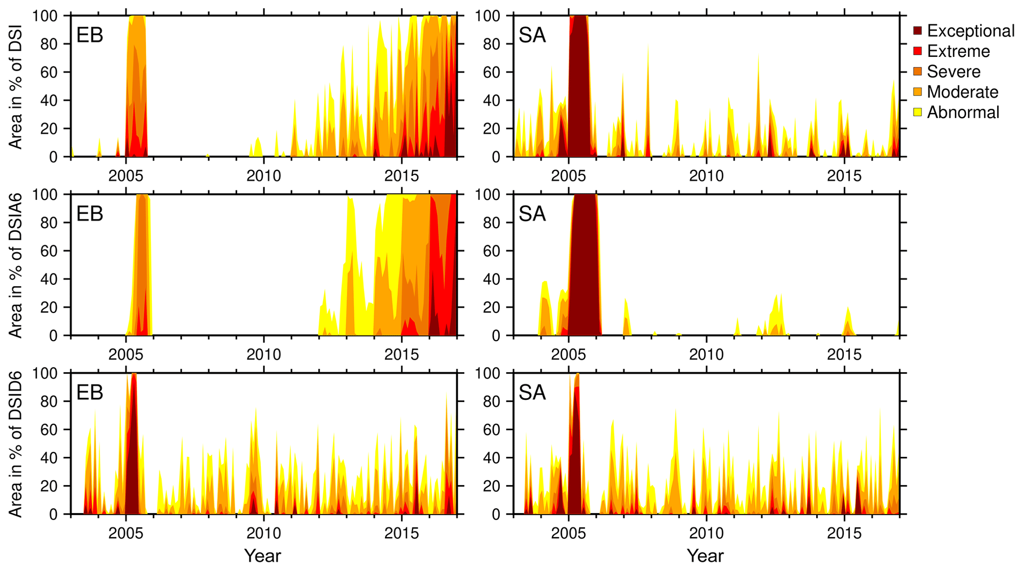
Figure 10Drought-affected area of the DSI, DSIA, and DSID (%) considering the different drought severity classes within the clusters of eastern Brazil (EB) and southern Africa (SA).
We note that large differences are found between DSI, the 6-month accumulated DSIA, and the 6-month differenced DSID within the given drought period for the eastern Brazil region (Fig. 10, left). All three indicators manage to identify the drought, but they also do so with a different duration and percentage of the affected area. Within the simulated drought period, the DSI indicator identified no more than 14 % of all grid cells as being affected by exceptional drought where it should be 100 %. On the other hand, the DSIA does not detect exceptional drought in any grid cell. It is apparent that this indicator misses the exceptional dry event because of the included trend and acceleration.
When comparing the DSIA of eastern Brazil to the DSIA of southern Africa (Fig. 10, center), we find that DSIA is able to detect the drought strength correctly when there is a small trend or acceleration present. However, DSIA appears more robust against spatial noise, since it identifies severe drought or drier in more than 90 % of grid cells, while the DSI indicator identifies only about 60 %. As described in Sect. 4.1, longer accumulation periods lead to smoother and thus more robust indicators. We find that the DSID is more successful in detecting exceptional drought: more than 80 % of the DSID grid cells show exceptional drought, but the indicator appears more noisy than DSIA. Finally, with regard to the drought duration, we find that only DSI detects the true period correctly. When identified via DSIA, the duration appears longer, and when identified in DSID, the period was found shorter as compared to the true drought period.
Overall, we find that the different indicators of DSI, DSIA, and DSID all come with advantages and disadvantages regarding the presence of spatial and temporal noise. The same findings were made for the indicators of the Houborg method (results not shown). This analysis is not applied to the Thomas method, because the method does not refer to severity classes (Sect. 2.3).
4.3 Synthetic TWSC: experiments with variable trend, drought duration, and severity
Two experiments were additionally constructed to examine the influence of trends and drought parameters on the indicator capability. First, we consider how strong a linear trend in total water storage must be to mask drought in the indicators. For this, we test different trends from −10 to 10 mm yr−1 for DSI, DSIA, DI, DIA, and the Thomas method in the western India region (since these indicators were identified as being affected by trends; Sect. 4.1). No acceleration is included for these tests. We find that trends between −1 and 1 mm yr−1 cause no influence on all indicators, while differences start to appear when simulating a trend higher than 2 mm yr−1. This propagates into the DSI, DSIA, DI, and DIA indicators but did not affect the drought period.
A question we must ask is what would be the largest trend magnitude that does not affect the correct detection of drought duration and drought severity, and how can we verify this. An obvious influence within the drought period in 2005 is found when simulating a trend of −7 mm or lower per year. It is important at this point to understand that there is a relation between the timing of the drought and the sign of the trend, i.e., whether the trend is positive or negative. Assuming that a positive trend exists and the drought occurs closer to the end of the time series, the trend may lead to a drought that is identified as more dry than the true drought. But if the trend is negative, the drought is identified more easily.
Other factors, e.g., the length of the time series, have an influence on the masking by the trend and, as a result, affect drought detection. The longer the input time series, the more sensitive the drought detection is to the trend. At the same time, the magnitude of the trend needs to be considered relative to the variability or range of TWSC. For example, a −6 mm yr−1 trend has a larger influence on the drought detection if the range of TWSC is −50 to 50 mm compared to −200 to 200 mm. As a reference, the synthetic time series for western India, without any trend or acceleration signal, ranges from about −323 to 87 mm. So, deriving a general quantity for these dependencies is difficult.
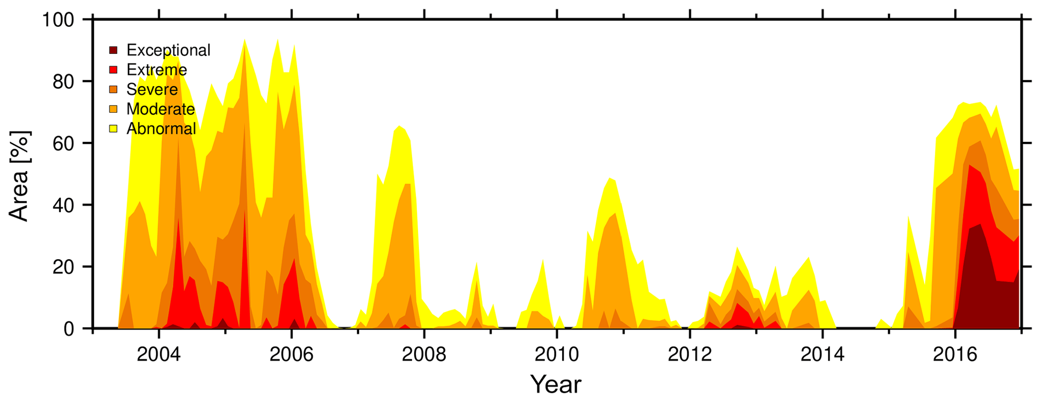
Figure 11Percentage of drought-affected area for the 6-month DSIA (–) considering the different drought severity classes. Application on real GRACE-TWSC over South Africa from 2003 to 2016.
In a second experiment, we assess which input drought duration and magnitude would at least be visually recognized in the indicators. We choose 3, 6, 9, 12, and 24 months for the simulated duration and −40, −60, −80, −100, and −120 mm for the drought magnitude and apply both the Zhao and the Houborg methods. We compare the changes for one indicator time series for the eastern Brazil region. The drought always begins in January 2005 for the first tests. In general, we found that the identification of the severity class is less sensitive to changes in the drought duration, since a drought duration of 3, 6, 9, 12, and 24 months mostly results in equal drought severity classes, for example, a drought magnitude of 120 mm. Thus, we concentrate our analysis on changes in drought magnitude.
Exceptional drought is only classified by the Zhao method for eastern Brazil for a simulated drought magnitude of 120 mm; this is related to the trend and acceleration signal contained in the simulated TWSC and was already found in Sect. 4.1. For the Zhao method, extreme drought is identified when simulating a drought magnitude of at least −100 mm, while only a period of severe and moderate drought is identified when simulating a magnitude of −80 and −60 mm. The Houborg method fails to identify extreme and exceptional drought, as described in Sect. 4.1. Thus, simulating a magnitude of −100 and −120 mm is identified as severe drought for all simulated drought periods (3 to 24 months), while simulating a lower magnitude (−80 and −60 mm) causes moderate or abnormal dry events to be identified. We find that both methods are not able to clearly detect a drought that has a magnitude of −40 mm or weaker if the duration is between 3 and 24 months. This experiment supports our findings in Sect. 3.2.
4.4 Application to real GRACE data: droughts in South Africa
For South Africa, droughts are a recurrent climatic phenomenon. The complex rainfall regime has led to multiple occurrences of drought events in the past, for example to a strong drought in 1983 (e.g., Rouault and Richard, 2003; Vogel et al., 2010; Malherbe et al., 2016). These past droughts appeared in varying climate regions, at different times of the year, and with a different severity. Since 1960, many of them were linked to El Niño (e.g., Rouault and Richard, 2003; Malherbe et al., 2016).
Based on the simulation results, we chose the 6-month accumulated DSIA to identify droughts for (the administrative area of) South Africa (GADM, 2018) in the GRACE total water storage data. DSIA has proven to be more robust with respect to the peculiar, GRACE-typical spatial and temporal noise as compared to the other tested indicators (Sect. 4.1 and 4.2).
GRACE-DSIA6 suggests two drought periods, from mid-2003 to mid-2006 and from 2015 to 2016 (Fig. 11). The first drought event is identified to affect at least 70 % of the area of South Africa. While 2003 was indeed a year of abnormal-to-severe dry conditions, extreme drought occurred during the period of 2004 to mid-2006. Figure 11 reveals that a small area (about 7976 km2, close to Lesotho) even experienced exceptional drought during 2004. This period is confirmed by the Emergency Events Database (EM-DAT, 2018) recording of a drought event in 2004 (e.g., Masih et al., 2014). Extreme drought in 2004 mainly occurred in central and southeastern South Africa; this is exemplified in Fig. 12a for April 2004. Another confirmation is found in Malherbe et al. (2016), who identified a drought period from 2003 to 2007 by using the SPI.
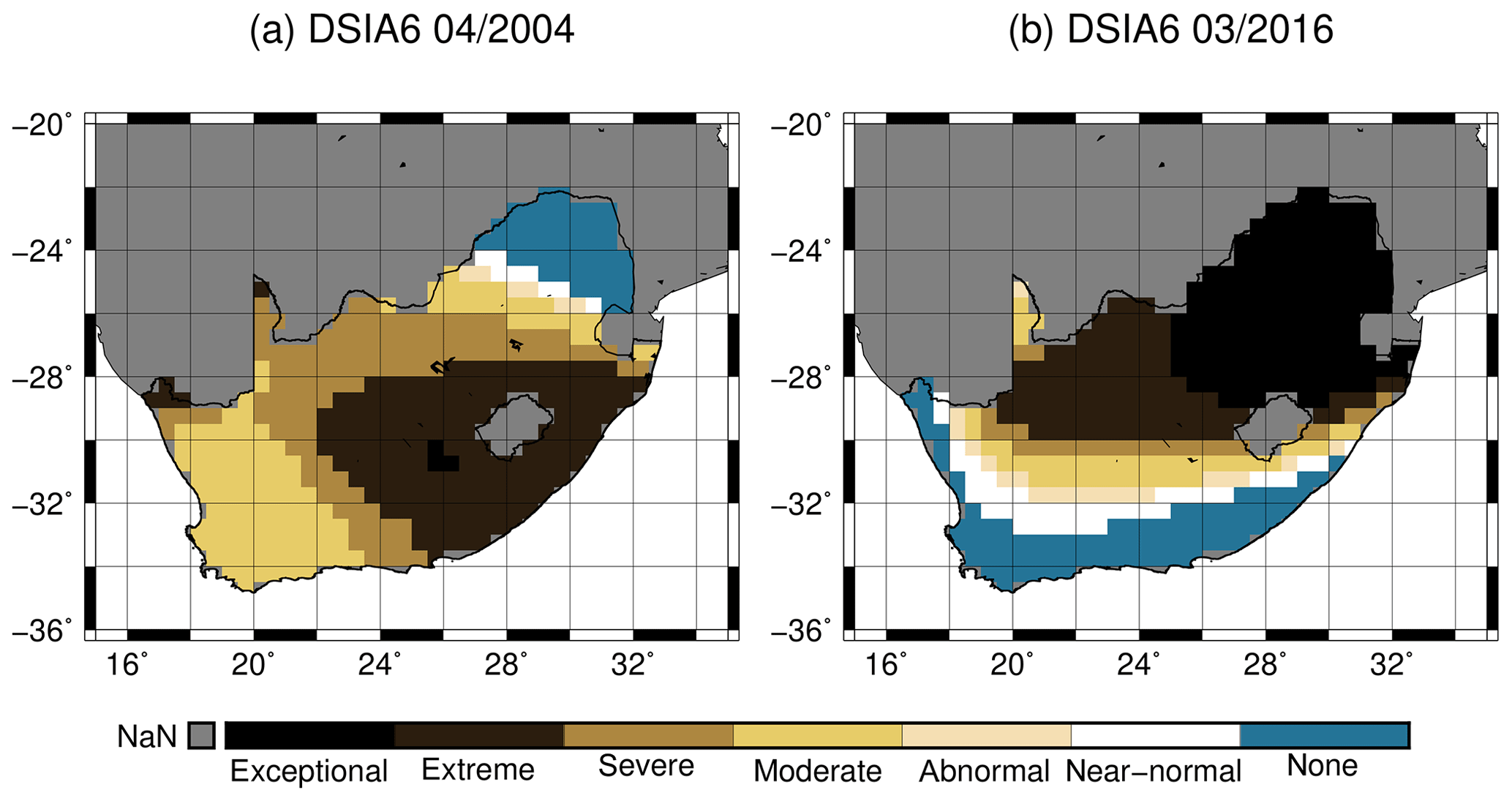
Despite affecting less area (about 50 % to 70 %; Fig. 11), the second drought in 2015 and 2016 is perceived as more intense than the drought from 2003 to 2006. Based on the GRACE-DSIA6 data, we conclude that in 2016 at least 30 % of South Africa was affected by extreme drought and about 20 % experienced an exceptional drought. The 2016 drought occurred in the northeastern part of South Africa (Fig. 12b). For comparison, the EM-DAT database similarly identified 2015 as a drought event, but it did not classify 2016 as such. We speculate that the differences are due to the drought criteria of EM-DAT (disasters are included when, for example, 10 or more people died or 100 or more people were affected). However, EM-DAT lists 2016 as a year of extreme temperature, which might be related to our detected drought. Furthermore, we can confirm the 2015–2016 drought is marked by a lower maximum precipitation in these years than in other years (about 65 mm) and by meteorological indicators indicating a period of severe-to-extreme drought (SPI; Standardized Precipitation Evapotranspiration Index; Vincente-Serrano et al., 2010; Weighted Anomaly Standardized Index; Lyon and Barnston, 2015).
The framework developed in this study enables us to simulate GRACE-TWSC data with realistic signal and noise properties and thus to assess the ability of GRACE drought indicators to detect drought events in a controlled environment with known truth. This will be extended to GRACE-FO in the near future. GRACE studies have often been based on simplified noise models (e.g., Zaitchik et al., 2008; Girotto et al., 2016), where the GRACE noise model is not derived from the used GRACE data but, for example, from literature and assumed to be spatially uniform and uncorrelated. However, it is important to account for realistic error and signal correlation (e.g., Eicker et al., 2014), in particular for drought studies where one will push the limits of GRACE spatial resolution. This signal correlation includes information about, for example, the geographic latitude, the density of the satellite orbits, the time dependencies of mission periods or north–south dependencies.
However, identifying a drought signal from real GRACE-TWSC data is indeed challenging since we do not know in advance what the signature of a drought looks like; a parametric drought model does not yet exist, and our experiment (Sect. 3.2) to extract such a model from TWSC data and known droughts did not lead to conclusive results. Still we believe that this first – to our knowledge – approach, despite being based on a small number of drought periods, identified a similar systematic behavior of different drought periods and should be pursued further. Based on literature and our own experiments (Sect. 4.3) we chose to define our “box”-like GRACE drought model as an immediate and constant water storage deficit.
When analyzing the Zhao, Houborg, and Thomas methods, we find that trends and accelerations in GRACE water storage maps tend to bias not only DSI, DI, and the Thomas indicator (which use non-climatological TWSC) but also DSIA and DIA (which use accumulated TWSC). The indicators DSID and DID, which utilize time-differenced TWSC, were not found to be biased by trends and accelerations; the same goes for the Thomas method when based on detrended and deseasoned TWSC. When we simulated smaller trends or accelerations, all indicators were able to detect drought, but they identified a different timing, duration, and strength, for example for the SA cluster (trend of 4.98 mm yr−1, acceleration of −0.38 mm yr−2). This suggests removing the trend in GRACE data first, but this must be done with care, since it can also influence the detection of, for example, long-term droughts. The same is true for removing the trend and seasonal signal prior of applying the Thomas method, although in this study we found that the removal of these signals simplified the correct drought detection (Sect. 4.1).
An experiment was then set up to understand the influence of the trend on the detected drought duration and severity. Several factors play a role here, e.g., the length of the time series, the TWSC range in relation to the trend magnitude, and the sign of the trend. We found that providing a general rule appears nearly impossible.
As expected, we find time series for the modified time-differencing GRACE indicators DSID and DID as much noisier when compared to the time-accumulating indicators DSIA and DIA; this can be linked to precipitation (Sect. 2) driving total water storage. The drought period was identified to be shorter than the true simulated drought period, e.g., for DSID3 and DSID6. After these drought periods, strongly wet periods were detected. Regarding future applications, we suggest a direct comparison of the DSID and meteorological indicators, in particular for confirming or rejecting drought duration and the following wet periods.
On the other hand, computing accumulated indicators implies a temporal smoothing causing the drought period to appear lagged in time; however for accumulation periods of 3 and 6 months the lag was found to be insignificant. DSIA and DIA are thus more robust against temporal and spatial GRACE noise as compared to DSID and DID, and again we would suggest utilizing 3 or 6 months accumulation periods. In general, we found the Zhao and Thomas indicators performed better in detecting the correct drought strength than the Houborg method, at least for the limited duration of the GRACE time series that we have at the time of writing.
By simulating the effect of spatial noise on drought detection, we found that some indicators appear less robust. Analysis of the percentage of the drought-affected area showed that the GRACE spatial noise limits correct drought detection. Again, DSIA was identified to be more robust compared to DSI and DSID – it was the only indicator that identified exceptional drought in nearly all grid cells. A second experiment was conducted to examine if the influence of the spatial noise can be reduced by using spatial averages. We found that spatially averaging DSI and DI appears less robust against the spatial noise compared to computing the indicator of the averaged TWSC. At this point we therefore suggest to compute the indicator from the spatially averaged TWSC. Since DI showed stronger difference between both averaging methods than DSI, we conclude that DI is generally less robust against spatial noise than DSI. In our real-data case study, due to these findings, the DSIA6 was thus applied to GRACE-TWSC, and it identified two drought periods: mid-2003 to mid-2006 in central and southeastern South Africa and 2015 to 2016 in northeastern South Africa.
A framework has been developed that enables a better understanding of the masking of drought signals when applying the methods of Zhao et al. (2017), Houborg et al. (2012), and Thomas et al. (2014). Four new GRACE-based indicators (DSIA, DSID, DIA, and DID) were derived and tested; these are modifications of the above mentioned approaches based on time-accumulated and time-differenced GRACE data. We found that indeed most indicators were mainly sensitive to water storage trends and to the GRACE-typical spatial noise.
Among these various indicators, we identified the DSIA6 as particularly well-performing; i.e., it is less sensitive to GRACE noise and is well capable of identifying the correct severity of drought, at least in absence of trends. However, the choice of the indicator should always be made in the context of the application.
We see ample possibilities to extend our framework. Future work should focus on better defining the onset and end of a drought and developing a signature for a TWSC drought. One should also consider other observable measurements in the simulation, such as groundwater for example, which can be derived from GRACE and by removing other storage contributions from direct modeling or through data assimilation.
In the GRACE community, efforts are currently being made to “bridge” the GRACE time series to the beginning of the GRACE-FO data period (e.g., Jäggi et al., 2016; Lück et al., 2018). These gap-filling data will inevitably have much higher noise and spatial correlations that may be very different from GRACE data, and drought detection capability should be investigated through simulation first. On the other hand, GRACE-FO is supposed to provide more precise measurements, and thus less influence of spatial noise on the drought detection may be expected. The combination of GRACE-FO data and a thorough understanding and “tuning” of GRACE drought identification methods, possibly through this framework, might then enable us to identify water storage droughts more precisely.
To extract temporal correlations from the GRACE total water storage changes we apply an autoregressive model, which is described by
where X represents the observed process at time t, p is the model order, ϕ is the correlation parameters, and ϵ is a white-noise process (Akaike, 1969). Here, detrended and deseasoned TWSC are used as the observed process X(t) because the remaining residuals contain interannual and subseasonal signal data as the drought information, which we want to extract with this approach. The approach is then applied for different model orders. The optimal order of the AR model is adjusted by means of the information criteria, for example the Akaike information criterion (AIC) and the Bayesian information criterion (BIC). Then, by using the optimal order, the AR model coefficients ϕ, which represent the temporal correlations, can be computed using a least squares adjustment.
The results for the optimal order of interannual and subseasonal TWSC is shown in Fig. A1. Most of the global land grids of detrended and deseasoned TWSC show an optimal order of 1 (about 70 %).
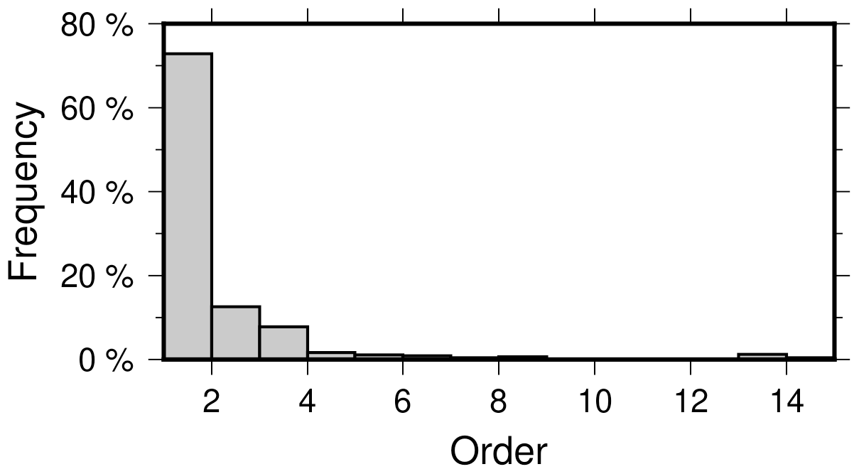
Figure A1Histogram of the optimal order of an AR model for global detrended and deseasoned GRACE-TWSC on land grids.
Expectation maximization represents a popular iterative algorithm that is widely used for clustering data. EM partitions data into clusters of different sizes and aims at finding the maximum likelihood of parameters of a predefined probability distribution (Dempster et al., 1977). In the case of a Gaussian distribution the EM algorithm maximizes the Gaussian mixture parameters, which are the Gaussian mean μk, covariance Σk, and mixing coefficients πk (Szeliski, 2010). The algorithm then iteratively applies two consecutive steps to maximize the parameters: the expectation step (E step) and the maximization step (M step). Within the E step we estimate the likelihood that a data point xt is generated from the kth Gaussian mixture by
The M step then re-estimates the parameters for each Gaussian mixture as follows:
by using the number of points assigned to each cluster via
Using the maximized parameters, EM assigns each data point to a cluster. The final global distributed clusters of the AR parameters (Fig. 3) are shown in Fig. B1. These clusters were derived by modifying and applying an EM algorithm provided by Chen (2018).
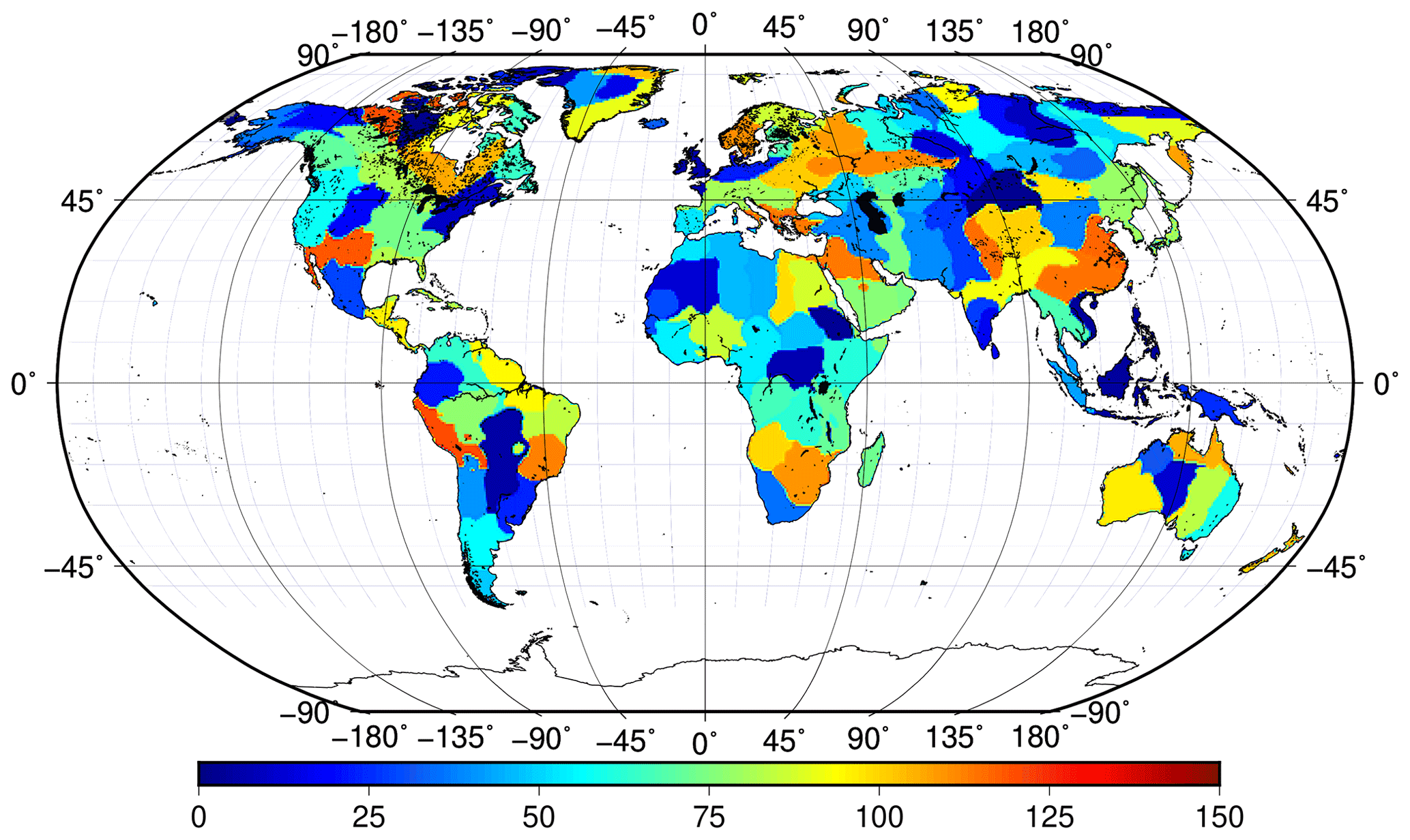
Figure B1Clusters based on EM clustering applied to the global AR model coefficients.
The decomposition of the variance–covariance matrix Σ by using Cholesky decomposition fails when Σ is positive semi-definite. To still be able to decompose the matrix, we can use eigenvalue decomposition, but this is accompanied by a loss of information due to the rank deficiency. The decomposition is then examined by Σ=UDUT, where U is a matrix with the eigenvectors of Σ in each column and D is a diagonal matrix of the eigenvalues. In this case, a decomposed matrix can be related to RT introduced in Sect. 3.1. RT can be computed by . In Sect. 3.1, we multiply RT with a normal distributed noise time series of the same length as the rows of Σ. In this case, the number of normal distributed noise time series n is then replaced by the rank of Σ.
GRACE-TWSCs are freely available at http://skylab.itg.uni-bonn.de/data_and_models/grace/hydrology/total_water_storage/ (Gerdener et al., 2019). Information about the postprocessing of the data can be found at https://www.apmg.uni-bonn.de/daten-und-modelle/grace-monthly-solutions (Gerdener et al., 2018).
HG, OE, and JK designed all computations, and HG carried them out. HG prepared the paper with contributions from OE and JK.
The authors declare that they have no conflict of interest.
We acknowledge the funding from the German Federal Ministry of Education and Research (BMBF) for the “GlobeDrought” project through its funding measure Global Resource Water (GRoW).
This research has been supported by the Bundesministerium für Bildung und Forschung (grant no. 02WGR1457A).
This paper was edited by Bettina Schaefli and reviewed by two anonymous referees.
A, G., Wahr, J., Zhong, S.: Computations of the viscoelastic response of a 3-D compressible Earth to surface loading: an application to Glacial Isostatic Adjustment in Antarctica and Canada, Geophys. J. Int., 192, 557–572, 2013. a
Agboma, C. O., Yirdaw, S. Z. and Snelgrove, K. R.: Intercomparison of the total storage deficit index (TSDI) over two Canadian Prairie catchments, J. Hydrol., 374, 351–359, https://doi.org/10.1016/j.jhydrol.2009.06.034, 2009. a
Akaike, H.: Fitting autoregressive models for prediction, Ann. Inst. Stat. Math., 21, 243–247, https://doi.org/10.1007/BF02532251, 1969. a, b
Alpaydin, E.: Introduction to machine learning, MIT Press, Cambridge, Massachusetts, USA, 2009. a
Andersen, O. B., Seneviratne, S. I., Hinderer, J. and Viterbo, P.: GRACE-derived terrestrial water storage depletion associated with the 2003 European heat wave, Geophys. Res. Lett., 32, L18405, https://doi.org/10.1029/2005GL023574, 2005. a, b
Bachmair, S., Stahl, K., Collins, K., Hannaford, J., Acreman, M., Svoboda, M., Knutson, C., Smith, K. H., Wall, N., Fuchs, B., Crossman, N. D. and Overton, I. C.: Drought indicators revisited: the need for a wider consideration of environment and society: Drought indicators revisited, Wiley Interdisciplin. Rev.: Water, 3, 516–536, https://doi.org/10.1002/wat2.1154, 2016. a
Changnon, S. A.: Detecting Drought Conditions in Illinois, Circular 169, Illinois State Water Survey, Champaign, 1987. a, b
Checchi, F. and Robinson, W. C.: Mortality among populations of southern and central Somalia affected by severe food insecurity and famine during 2010–2012, Food and Agriculture Organization of the United Nations, Rome, Washington, 2013. a
Chen, J. L., Wilson, C. R., Tapley, B. D., Yang, Z. L. and Niu, G. Y.: 2005 drought event in the Amazon River basin as measured by GRACE and estimated by climate models, J. Geophys. Res., 114, B05404, https://doi.org/10.1029/2008JB006056, 2009. a, b, c, d
Chen, J. L., Wilson, C. R., Tapley, B. D., Longuevergne, L., Yang, Z. L., and Scanlon, B. R.: Recent La Plata basin drought conditions observed by satellite gravimetry, J. Geophys. Res., 115, D22108, https://doi.org/10.1029/2010JD014689, 2010. a
Chen, M.: EM Algorithm for Gaussian Mixture Model (EM GMM), MATLAB Central File Exchange, available at: https://www.mathworks.com/matlabcentral/fileexchange/26184-em-algorithm-for-gaussian-mixture-model-em-gmm, lst access: September 2018. a, b
Cheng, M., Ries, J. C. and Tapley, B. D.: Variations of the Earth's figure axis from satellite laser ranging and GRACE, J. Geophys. Res., 116, B01409, https://doi.org/10.1029/2010JB000850, 2011. a
Coelho, C. A. S., de Oliveira, C. P., Ambrizzi, T., Reboita, M. S., Carpenedo, C. B., Campos, J. L. P. S., Tomaziello, A. C. N., Pampuch, L. A., Custódio, M. de S., Dutra, L. M. M., Da Rocha, R. P., and Rehbein, A.: The 2014 southeast Brazil austral summer drought: regional scale mechanisms and teleconnections, Clim. Dynam., 46, 3737–3752, https://doi.org/10.1007/s00382-015-2800-1, 2016. a
Dempster, A. P., Laird, N. M., and Rubin, D. B.: Maximum Likelihood from Incomplete Data via the EM Algorithm, J. Roy. Stat. Soc., 39, 1–38, 1977. a, b, c
Eicker, A., Schumacher, M., Kusche, J., Döll, P., and Schmied, H. M.: Calibration/Data Assimilation Approach for Integrating GRACE Data into the WaterGAP Global Hydrology Model (WGHM) Using an Ensemble Kalman Filter: First Results, Surv. Geophys., 35, 1285–1309, https://doi.org/10.1007/s10712-014-9309-8, 2014. a, b
Eicker, A., Forootan, E., Springer, A., Longuevergne, L., and Kusche, J.: Does GRACE see the terrestrial water cycle “intensifying”: Water Cycle Intensification With GRACE, J. Geophys. Res.-Atmos., 121, 733–745, https://doi.org/10.1002/2015JD023808, 2016. a
EM-DAT: The Emergency Events Database, Université catholique de Louvain (UCL) – CRED, D. Guha-Sapir, Brussels, Belgium, available at: https://www.emdat.be/, last access: 5 December 2018. a
Espinoza, J. C., Ronchail, J., Guyot, J. L., Junquas, C., Vauchel, P., Lavado, W., Drapeau, G., and Pombosa, R.: Climate variability and extreme drought in the upper Solimões River (western Amazon Basin): Understanding the exceptional 2010 drought, Geophysical Research Letters, 38, L13406, https://doi.org/10.1029/2011GL047862, 2011. a, b, c
Frappart, F., Papa, F., Santos da Silva, J., Ramillien, G., Prigent, C., Seyler, F., and Calmant, S.: Surface freshwater storage and dynamics in the Amazon basin during the 2005 exceptional drought, Environ. Res. Lett., 7, 044010, https://doi.org/10.1088/1748-9326/7/4/044010, 2012. a
Frappart, F., Ramillien, G., and Ronchail, J.: Changes in terrestrial water storage versus rainfall and discharges in the Amazon basin, Int. J. Climatol., 33, 3029–3046, https://doi.org/10.1002/joc.3647, 2013. a, b, c, d
GADM database: version 3.4, available at: https://www.gadm.org/ (last access: 13 January 2020), 2018. a, b
Gerdener, H., Schulze, K., Yakhontova, A., Engels, O., and Kusche, K.: Description of post-processing steps for generating GRACE Level-3 monthly solutions, available at: https://www.apmg.uni-bonn.de/daten-und-modelle/grace-monthly-solutions (last access: 16 January 2020), 2018. a
Gerdener, H., Schulze, K., Yakhontova, A., Engels, O., and Kusche, K.: GRACE Level-3 monthly solutions, available at: http://skylab.itg.uni-bonn.de/data_and_models/grace/hydrology/total_water_storage/ (last access: 16 January 2020), 2019. a
Girotto, M., De Lannoy, G. J. M., Reichle, R. H., and Rodell, M.: Assimilation of gridded terrestrial water storage observations from GRACE into a land surface model, Water Resour. Res., 52, 4164–4183, https://doi.org/10.1002/2015WR018417, 2016. a, b
Houborg, R., Rodell, M., Li, B., Reichle, R., and Zaitchik, B. F.: Drought indicators based on model-assimilated Gravity Recovery and Climate Experiment (GRACE) terrestrial water storage observations, Water Resour. Res., 48, W07525, https://doi.org/10.1029/2011WR011291, 2012. a, b, c, d, e, f, g, h, i
Humphrey, V., Gudmundsson, L., and Seneviratne, S. I.: Assessing Global Water Storage Variability from GRACE: Trends, Seasonal Cycle, Subseasonal Anomalies and Extremes, Surv. Geophys., 37, 357–395, https://doi.org/10.1007/s10712-016-9367-1, 2016. a, b, c, d, e
IPCC: Climate Change 2013: The Physical Science Basis, in: Contribution of Working Group I to the Fifth Assessment Report of the Intergovernmental Panel on Climate Change, edited by: Stocker, T. F., Qin, D., Plattner, G.-K., Tignor, M., Allen, S. K., Boschung, J., Nauels, A., Xia, Y., Bex, V., and Midgley, P. M., Cambridge University Press, Cambridge, UK and New York, NY, USA, 1535 pp., 2013. a
Jäggi, A., Dahle, C., Arnold, D., Bock, H., Meyer, U., Beutler, G., and van den IJssel, J.: Swarm kinematic orbits and gravity fields from 18 months of GPS data, Adv. Space Res., 57, 218–233, https://doi.org/10.1016/j.asr.2015.10.035, 2016. a
Keyantash, J. and Dracup, J. A.: The Quantification of Drought: An Evaluation of Drought Indices, B. Am. Meteorol. Soc., 83, 1167–1180, 2002. a, b
Kusche, J., Schmidt, R., Petrovic, S., and Rietbroek, R.: Decorrelated GRACE time-variable gravity solutions by GFZ, and their validation using a hydrological model, J. Geod., 83, 903–913, https://doi.org/10.1007/s00190-009-0308-3, 2009. a
Kusche, J., Eicker, A., Forootan, E., Springer, A., and Longuevergne, L.: Mapping probabilities of extreme continental water storage changes from space gravimetry, Geophys. Res. Lett., 43, 8026–8034, https://doi.org/10.1002/2016GL069538, 2016. a
Long, D., Scanlon, B. R., Longuevergne, L., Sun, A. Y., Fernando, D. N., and Save, H.: GRACE satellite monitoring of large depletion in water storage in response to the 2011 drought in Texas, Geophys. Res. Lett., 40, 3395–3401, https://doi.org/10.1002/grl.50655, 2013. a, b
Lück, C., Kusche, J., Rietbroek, R., and Löcher, A.: Time-variable gravity fields and ocean mass change from 37 months of kinematic Swarm orbits, Solid Earth, 9, 323–339, https://doi.org/10.5194/se-9-323-2018, 2018. a
Lyon, B. and Barnston, A. G.: ENSO and the Spatial Extent of Interannual Precipitation Extremes in Tropical Land Areas, J. Climate, 18, 5095–5109, https://doi.org/10.1175/JCLI3598.1, 2005. a
Malherbe, J., Dieppois, B., Maluleke, P., Van Staden, M., and Pillay, D. L.: South African droughts and decadal variability, Nat. Hazards, 80, 657–681, https://doi.org/10.1007/s11069-015-1989-y, 2016. a, b, c
Mann, M. E. and Gleick, P. H.: Climate change and California drought in the 21st century, P. Natl. Acad. Sci. USA, 112, 3858–3859, https://doi.org/10.1073/pnas.1503667112, 2015. a
Masih, I., Maskey, S., Mussá, F. E. F., and Trambauer, P.: A review of droughts on the African continent: a geospatial and long-term perspective, Hydrol. Earth Syst. Sci., 18, 3635–3649, https://doi.org/10.5194/hess-18-3635-2014, 2014. a
Mayer-Gürr, T., Behzadpour, S., Ellmer, M., Kvas, A., Klinger, B., and Zehentner, N.: ITSG-Grace2016 – Monthly and Daily Gravity Field Solutions from GRACE, GFZ Data Services, https://doi.org/10.5880/icgem.2016.007, 2016. a
McKee, T. B., Doesken, N. J., and Kleist, J.: The relationship of drought frequency and duration to time scales, American Meteorolocial Society, Anaheim, CA, 179–183, 1993. a, b
Mishra, A. K. and Singh, V. P.: A review of drought concepts, J. Hydrol., 391, 202–216, https://doi.org/10.1016/j.jhydrol.2010.07.012, 2010. a, b, c
Moore, J., Woods, M., Ellis, A. and B. Moran, B.: Aerial survey results: California, Region 5, USDA Forest Service, 2016. a
Parthasarathy, B., Sontakke, N. A., Monot, A. A., and Kothawale, D. R.: Droughts/floods in the summer monsoon season over different meteorological subdivisions of India for the period 1871–1984, J. Climatol., 7, 57–70, 1987. a
Rebetez, M., Mayer, H., Dupont, O., Schindler, D., Gartner, K., Kropp, J. P., and Menzel, A.: Heat and drought 2003 in Europe: a climate synthesis, Ann. of Forest Sci., 63, 569–577, https://doi.org/10.1051/forest:2006043, 2006. a
Redner, R. A. and Walker, H. F.: Mixture Densities, Maximum Likelihood and the EM Algorithm, SIAM Rev., 26, 195–239, https://doi.org/10.1137/1026034, 1984. a, b
Rodell, M., Famiglietti, J. S., Wiese, D. N., Reager, J. T., Beaudoing, H. K., Landerer, F. W.. and Lo, M.-H.: Emerging trends in global freshwater availability, Nature, 557, 651–659, https://doi.org/10.1038/s41586-018-0123-1, 2018. a
Rouault, M. and Richard, Y.: Intensity and spatial extension of drought in South Africa at different time scales, Water SA, 29, 489–500, 2003. a, b, c
Rouault, M. and Richard, Y.: Intensity and spatial extent of droughts in southern Africa, Geophys. Res. Lett., 32, L15702, https://doi.org/10.1029/2005GL022436, 2005. a
Seitz, F., Schmidt, M. and Shum, C. K.: Signals of extreme weather conditions in Central Europe in GRACE 4-D hydrological mass variations, Earth Planet. Sc. Lett., 268, 165–170, https://doi.org/10.1016/j.epsl.2008.01.001, 2008. a, b, c, d
Springer, A.: A water storage reanalysis over the European continent: assimilation of GRACE data into a high-resolution hydrological model and validation, PhD thesis, Rheinische Friedrich-Wilhelms Universität Bonn, Bonn, urn:nbn:de:hbz:5n-53930, 2019. a
Swenson S. C., Chambers, D. P., and Wahr, J.: Estimating geocenter variations from a combination of GRACE and ocean model output, J. Geophys. Res.-Solid, 113, B08410, https://doi.org/10.1029/2007JB005338, 2008. a
Szeliski, R.: Computer Vision: Algorithms and Applications, Springer Science and Business Media, London, 2010. a
Thomas, A. C., Reager, J. T., Famiglietti, J. S., and Rodell, M.: A GRACE-based water storage deficit approach for hydrological drought characterization, Geophys. Res. Lett., 41, 1537–1545, https://doi.org/10.1002/2014GL059323, 2014. a, b, c, d, e, f, g, h, i, j
Tsakiris, G.: Drought Risk Assessment and Management, Water Resour. Manage., 31, 3083–3095, https://doi.org/10.1007/s11269-017-1698-2, 2017. a, b
Van Loon, A. F.: Hydrological drought explained: Hydrological drought explained, Wiley Interdisciplin. Rev.: Water, 2, 359–392, https://doi.org/10.1002/wat2.1085, 2015. a
Vicente-Serrano, S. M., Beguería, S. and López-Moreno, J. I.: A Multiscalar Drought Index Sensitive to Global Warming: The Standardized Precipitation Evapotranspiration Index, J. Climate, 23, 1696–1718, https://doi.org/10.1175/2009JCLI2909.1, 2010. a
Vogel, C., Koch, I. and Van Zyl, K.: “A Persistent Truth” – Reflections on Drought Risk Management in Southern Africa, Weather Clim. Soc., 2, 9–22, https://doi.org/10.1175/2009WCAS1017.1, 2010. a
Voss, K. A., Famiglietti, J. S., Lo, M., de Linage, C., Rodell, M., and Swenson, S. C.: Groundwater depletion in the Middle East from GRACE with implications for transboundary water management in the Tigris-Euphrates-Western Iran region, Water Resour. Res., 49, 904–914, https://doi.org/10.1002/wrcr.20078, 2013. a
Wahr, J., Molenaar, M., and Bryan, F.: Time variability of the Earth's gravity field: Hydrological and oceanic effects and their possible detection using GRACE, J. Geophys. Res.-Solid, 103, 30205–30229, https://doi.org/10.1029/98JB02844, 1998. a, b
Wilhite, D. A.: Droughts: A Global Assesment, Routledge, London, 2016. a, b
Yi, H. and Wen, L.: Satellite gravity measurement monitoring terrestrial water storage change and drought in the continental United States, Scient. Rep., 6, 19909, https://doi.org/10.1038/srep19909, 2016. a
Zaitchik, B. F., Rodell, M., and Reichle, R. H.: Assimilation of GRACE Terrestrial Water Storage Data into a Land Surface Model: Results for the Mississippi River Basin, J. Hydrometeorol., 9, 535–548, https://doi.org/10.1175/2007JHM951.1, 2008. a, b
Zargar, A., Sadiq, R., Naser, B., and Khan, F. I.: A review of drought indices, Environ. Rev., 19, 333–349, 2011. a
Zhang, Z., Chao, B. F., Chen, J., and Wilson, C. R.: Terrestrial water storage anomalies of Yangtze River Basin droughts observed by GRACE and connections with ENSO, Global Planet. Change, 126, 35–45, https://doi.org/10.1016/j.gloplacha.2015.01.002, 2015. a
Zhao, M., Velicogna, I., and Kimball, J. S.: A global gridded dataset of GRACE drought severity index for 2002–14: Comparison with PDSI and SPEI and a case of the Australia millenium drought, J. Hydrometeorol., 18, 2117–2129, 2017. a, b, c, d, e, f, g, h, i, j, k, l
- Abstract
- Introduction
- Indicators for hydrological drought
- Framework to derive synthetic TWSC for computing drought indicators
- Indicator-based drought identification with synthetic and real GRACE data
- Discussion
- Conclusions and outlook
- Appendix A: AR model coefficients computations
- Appendix B: EM clustering
- Appendix C: Eigenvalue decomposition
- Data availability
- Author contributions
- Competing interests
- Acknowledgements
- Financial support
- Review statement
- References
The requested paper has a corresponding corrigendum published. Please read the corrigendum first before downloading the article.
- Article
(7535 KB) - Full-text XML
- Abstract
- Introduction
- Indicators for hydrological drought
- Framework to derive synthetic TWSC for computing drought indicators
- Indicator-based drought identification with synthetic and real GRACE data
- Discussion
- Conclusions and outlook
- Appendix A: AR model coefficients computations
- Appendix B: EM clustering
- Appendix C: Eigenvalue decomposition
- Data availability
- Author contributions
- Competing interests
- Acknowledgements
- Financial support
- Review statement
- References