A novel approach for the assessment of morphological evolution based on observed water levels in tide-dominated estuaries

Assessing the impacts of both natural (e.g. tidal forcing from the ocean) and human-induced changes (e.g. dredging for navigation and land reclamation) on estuarine morphology is particularly important for the protection and management of the estuarine environment. In this study, a novel analytical approach is proposed for the assessment of estuarine morphological evolution in terms of tidally averaged depth on the basis of the observed water levels along the estuary. The key lies in deriving a relationship between wave celerity and tidal damping or amplification. For given observed water levels at two gauging stations, it is possible to have a first estimation of both wave celerity (distance divided by tidal travelling time) and tidal damping or amplification rate (tidal range difference divided by distance), which can then be used to predict the morphological changes via an inverse analytical model for tidal hydrodynamics. The proposed method is applied to the Lingdingyang Bay of the Pearl River Estuary, located on the southern coast of China, to analyse the historical development of the tidal hydrodynamics and morphological evolution. The analytical results show surprisingly good correspondence with observed water depth and volume in this system. The merit of the proposed method is that it provides a simple approach for understanding the decadal evolution of the estuarine morphology through the use of observed water levels, which are usually available and can be easily measured.

1 Introduction

Understanding the morphological changes in estuaries due to natural processes and human interventions is especially important with regard to sustainable water management and ecological impacts on the estuarine environment (Prandle, 2004; Schuttelaars et al., 2013; Winterwerp and Wang, 2013; Wang et al., 2015; Hoitink et al., 2017; Luan et al., 2017). In recent decades, human activities have been crucial factors affecting the morphological evolution in estuaries, and morphological responses of estuaries to human activities have attracted worldwide attention (Syvitski et al., 2009; Monge-Ganuzas et al., 2013; Du et al., 2016; van Maren et al., 2016; Jiang et al., 2017). In previous studies, aerial photographs, satellite images, topographic maps and cross-sectional profiles are the commonly used field data to explore the morphological adjustments with varied resolution and accuracy by means of either data-driven studies (e.g. Zhang et al., 2015; Wu et al., 2014; Z. Y. Wu et al., 2016; C. S. Wu et al., 2016) or process-based morphodynamic models (e.g. Guo et al., 2014, 2016; Luan et al., 2017). It is noted that these high-resolution and successive field data are rare or unavailable in most estuaries, especially because the determination of detailed morphological changes is usually time and energy consuming. Hence, the development of a simple yet effective approach for the assessment of decadal morphological evolution without the need for bathymetric data collection is desirable, which is especially the case for ungauged basins (Gisen and Savenije, 2015).

In a frictionless, prismatic channel of a constant cross section (or an ideal estuary with no damping or amplification), the classical formula for tidal wave propagation can be described by (e.g. Savenije, 2012)

$$\begin{array}{}\text{(1)}& c_{\mathrm{0}}=\sqrt{g\stackrel{\mathrm{‾}}{h}/r_{\mathrm{S}}},\end{array}$$

where c₀ is the classical wave speed, g is the acceleration due to gravity, $\stackrel{\mathrm{‾}}{h}$ is the tidally averaged and cross-sectionally averaged water depth and r_S is the storage width ratio accounting for the intertidal storage in tidal flats or marshes. Thus for a frictionless, prismatic channel or an ideal estuary, it is possible to derive an analytical expression for the stream depth, i.e. $\stackrel{\mathrm{‾}}{h}=r_{\mathrm{S}}{c}_{\mathrm{0}}^{\mathrm{2}}/g$, which is proportional to the square of the classical wave speed (Savenije and Veling, 2005). However, Eq. (1) does not apply in real alluvial estuaries due to the predominance of either morphological convergence or bottom friction. Thus, to have a first-order estimate of the stream depth, a relationship taking into account both tidal damping (or amplification) and channel convergence should be adopted. Such a relationship can be easily obtained from the recently published analytical solutions for tidal hydrodynamics in convergent estuaries (e.g. Savenije and Veling, 2005; Savenije et al., 2008; Toffolon and Savenije, 2011; van Rijn, 2011; Cai et al., 2012, 2016; Winterwerp and Wang, 2013).

Previous studies have clearly demonstrated that the behaviour of both the tidal damping (or amplification) and wave speed strongly depends on the degree of channel convergence and on the intensity of friction (e.g. Jay, 1991; Savenije and Veling, 2005). In particular, analytical solutions of tidal hydrodynamics are able to predict the main trends of tidal damping (or amplification) and wave speed for given forcing tidal amplitude, geometry (e.g. the spatially averaged depth and width convergence length) and friction (e.g. Prandle and Rahman, 1980; Friedrichs and Aubrey, 1994; Savenije et al., 2008; Toffolon and Savenije, 2011; van Rijn, 2011; Cai et al., 2012, 2016; Winterwerp and Wang, 2013). Conversely, if tidal damping (or amplification) and wave speed are known from observations, analytical models can be used to estimate the unknown tidally averaged depth and other tidal dynamics (e.g. velocity amplitude and phase difference between velocity and elevation). Following this line of thought, the main objective of this study is to provide an analytical framework to assess the morphological evolution of estuaries based on the tidally averaged depth derived from the observed tidal hydrodynamics (i.e. tidal damping or amplification and wave speed).

It is worth noting that considerable simplifications of geometry and forcing are made in order to derive generic analytical solutions of the governing Saint-Venant equations. Here, we restrict consideration to infinitely long tide-dominated estuaries with low tidal-amplitude-to-depth ratios and Froude numbers. The fundamental assumption is that the geometry (cross-sectional area, width and depth) of the channel can be described by a simple exponential function. We also assume that the velocity of river discharge is small compared to the tidal velocity. In this paper, we use the analytical relation of wave celerity, first proposed by Savenije and Veling (2005), to predict the estuarine morphological dynamics in terms of the large-scale geometrical properties of the estuary, i.e. the tidally averaged depth and volume based on the observed water levels through the estuary.

The Pearl River is the second-largest river in terms of water discharge in China (Liu et al., 2017) and drains into the South China Sea through Lingdingyang Bay, Modaomen Estuary and Huangmaohai Bay. In this study, we focus on Lingdingyang Bay, which is the largest of these tidal systems in terms of water area and consists of three major shoals and two channels. Previous studies have examined the morphological evolution of Lingdingyang Bay using satellite images (e.g. Wu et al., 2014), topographic maps (e.g. C. S. Wu et al., 2016; Z. Y. Wu et al., 2016) and cross-sectional profiles (Z. Y. Wu et al., 2016). Due to intensive human activities (e.g. land reclamation and channel dredging), significant morphological changes have occurred in Lingdingyang Bay in recent decades. As a consequence, the west and east shoals expanded towards the bay, and the two channels became narrower and deeper (Zhang et al., 2015; Z. Y. Wu et al., 2016). Furthermore, these morphological changes have resulted in changes in tidal dynamics (Zhang et al., 2010; Deng and Bao, 2011). Our study can provide a new method to explore the morphological evolution, which provides scientific guidelines for management and regulation projects in estuaries.

The paper is organized as follows. Section 2 describes the analytical method for reproducing the tidal hydrodynamics and an inverse model for predicting the tidally averaged depth. An overview of the study area is provided in Sect. 3. In Sect. 4, the morphological evolution of Lingdingyang Bay is described, and the proposed method is applied. Subsequently, the relationship between morphology and tidal dynamics is discussed, along with the model limitations (Sect. 5). Finally, some conclusions are drawn in Sect. 6.

2 Methodology and material

2.1 Analytical model for tidal hydrodynamics in an infinitely long channel

The depth-averaged equations for the conservation of mass and momentum in a channel with a gradually varying cross section can be described by (e.g. Savenije, 2005; van Rijn, 2011)

$$\begin{array}{}\text{(2)}& r_{\mathrm{S}}{\displaystyle \frac{\partial Z}{\partial t}}+U{\displaystyle \frac{\partial Z}{\partial x}}+h{\displaystyle \frac{\partial U}{\partial x}}+{\displaystyle \frac{hU}{\stackrel{\mathrm{‾}}{B}}}{\displaystyle \frac{\mathrm{d}\stackrel{\mathrm{‾}}{B}}{\mathrm{d}x}}=\mathrm{0},\end{array}$$

$$\begin{array}{}\text{(3)}& {\displaystyle \frac{\partial U}{\partial t}}+U{\displaystyle \frac{\partial U}{\partial x}}+g{\displaystyle \frac{\partial Z}{\partial x}}+{\displaystyle \frac{rU}{h}}=\mathrm{0},\end{array}$$

where U is the cross-sectionally averaged velocity, Z is the free surface elevation, h is the water depth, $\stackrel{\mathrm{‾}}{B}$ is the tidally averaged width (hereafter, overbars denote tidal averages), t is the time, x is the longitudinal coordinate measured positive in the landward direction (x=0 at the mouth) and r is the linearized friction factor defined as (Lorentz, 1926)

$$\begin{array}{}\text{(4)}& r={\displaystyle \frac{\mathrm{8}}{\mathrm{3}\mathit{\pi }}}{\displaystyle \frac{g\mathit{\upsilon }}{K^{\mathrm{2}}{\stackrel{\mathrm{‾}}{h}}^{\mathrm{1}/\mathrm{3}}}},\end{array}$$

where the coefficient 8∕(3π) stems from adopting Lorentz's linearization of the quadratic friction term (Lorentz, 1926) considering only one single predominant tidal constituent (e.g. M₂), and K is the Manning–Strickler friction coefficient.

To derive the analytical solution for the tidal hydrodynamics in convergent channels, it is assumed that the tidally averaged cross-sectional area $\stackrel{\mathrm{‾}}{A}$ and width $\stackrel{\mathrm{‾}}{B}$ can be described by the following exponential functions:

$$\begin{array}{}\text{(5)}& {\displaystyle }& {\displaystyle }\stackrel{\mathrm{‾}}{A}=\stackrel{\mathrm{‾}}{A_{\mathrm{0}}}\exp (-x/a),\text{(6)}& {\displaystyle }& {\displaystyle }\stackrel{\mathrm{‾}}{B}=\stackrel{\mathrm{‾}}{B_{\mathrm{0}}}\exp (-x/b),\end{array}$$

where $\stackrel{\mathrm{‾}}{A_{\mathrm{0}}}$ and $\stackrel{\mathrm{‾}}{B_{\mathrm{0}}}$ are the respective values at the estuary mouth and a and b are the convergence lengths of the cross-sectional area and width, respectively. The other fundamental assumption is that the flow is mainly concentrated in a rectangular cross section, with a possible influence from storage areas described by the storage width ratio r_S. It directly follows from the assumption of a rectangular cross section that the tidally averaged depth is given by $\stackrel{\mathrm{‾}}{h}=\stackrel{\mathrm{‾}}{A}/\stackrel{\mathrm{‾}}{B}$.

Considering a system that is forced by a sinusoidal tidal wave with period T and frequency $\mathit{\omega }=\mathrm{2}\mathit{\pi }/T$, the wave functions of water level and flow velocity are defined as

$$\begin{array}{}\text{(7)}& {\displaystyle }& {\displaystyle }Z=\mathit{\eta }\cos \left(\mathit{\omega }t-{\mathit{\varphi }}_Z\right),\text{(8)}& {\displaystyle }& {\displaystyle }U=\mathit{\upsilon }\cos \left(\mathit{\omega }t-{\mathit{\varphi }}_U\right),\end{array}$$

where η and υ are the wave amplitudes of elevation and velocity, respectively, while ϕ_Z and ϕ_U are their corresponding phases. As the wave propagates into the estuary, it has a wave celerity c and a phase lag ε, defined as the phase difference between high water (HW) and high-water slack (HWS) (or between low water – LW – and low-water slack – LWS). For a simple harmonic wave, $\mathit{\epsilon }=\mathit{\pi }/\mathrm{2}-({\mathit{\varphi }}_Z-{\mathit{\varphi }}_U)$. After scaling Eqs. (2) and (3) (see details in Appendix A), five dimensionless variables can be derived: the estuary shape number γ (representing the effect of cross-sectional area convergence), the friction number χ (describing the role of frictional dissipation), the velocity number μ (the actual velocity scaled with the frictionless value in a prismatic channel), the celerity number λ (the ratio between the theoretical frictionless celerity in a prismatic channel and the actual wave celerity) and the damping number for tidal amplitude δ (a dimensionless description of the increase, δ>0, or decrease, δ<0, of the tidal wave amplitude along the estuary), where γ and χ are the independent variables, while μ, λ and δ (together with ε) are the dependent variables. These dimensionless variables are defined as

$$\begin{array}{}\text{(9)}& {\displaystyle }& {\displaystyle }\mathit{\gamma }={\displaystyle \frac{c_{\mathrm{0}}}{\mathit{\omega }a}},\text{(10)}& {\displaystyle }& {\displaystyle }\mathit{\chi }=r_{\mathrm{S}}f{\displaystyle \frac{c_{\mathrm{0}}}{\mathit{\omega }}}\mathit{\zeta },\text{(11)}& {\displaystyle }& {\displaystyle }\mathit{\mu }={\displaystyle \frac{\mathrm{1}}{r_{\mathrm{S}}}}{\displaystyle \frac{\mathit{\upsilon }\stackrel{\mathrm{‾}}{h}}{\mathit{\eta }{c}_{\mathrm{0}}}},\text{(12)}& {\displaystyle }& {\displaystyle }\mathit{\lambda }={\displaystyle \frac{c_{\mathrm{0}}}{c}},\text{(13)}& {\displaystyle }& {\displaystyle }\mathit{\delta }={\displaystyle \frac{\mathrm{1}}{\mathit{\eta }}}{\displaystyle \frac{\mathrm{d}\mathit{\eta }}{\mathrm{d}x}}{\displaystyle \frac{c_{\mathrm{0}}}{\mathit{\omega }}},\end{array}$$

where f is the dimensionless friction factor, and ζ is the dimensionless tidal amplitude defined as

$$\begin{array}{}\text{(14)}& {\displaystyle }& {\displaystyle }f={\displaystyle \frac{g}{K^{\mathrm{2}}{\stackrel{\mathrm{‾}}{h}}^{\mathrm{1}/\mathrm{3}}}}{\left(\mathrm{1}-(\mathrm{1.33}\mathit{\zeta }{)}^{\mathrm{2}}\right)}^{-\mathrm{1}},\text{(15)}& {\displaystyle }& {\displaystyle }\mathit{\zeta }={\displaystyle \frac{\mathit{\eta }}{\stackrel{\mathrm{‾}}{h}}}.\end{array}$$

Making use of these dimensionless parameters, Cai et al. (2012), building on the previous work by Savenije et al. (2008), showed that the analytical solution of the tidal hydraulic equations can be obtained by solving a set of four implicit equations, i.e. the phase lag equation (Eq. 16), the scaling equation (Eq. 17), the damping equation (Eq. 18) and the celerity equation (Eq. 19):

$$\begin{array}{}\text{(16)}& {\displaystyle }& {\displaystyle }\tan \left(\mathit{\epsilon }\right)={\displaystyle \frac{\mathit{\lambda }}{\mathit{\gamma }-\mathit{\delta }}},\text{(17)}& {\displaystyle }& {\displaystyle }\mathit{\mu }={\displaystyle \frac{\sin \left(\mathit{\epsilon }\right)}{\mathit{\lambda }}}={\displaystyle \frac{\cos \left(\mathit{\epsilon }\right)}{\mathit{\gamma }-\mathit{\delta }}},\text{(18)}& {\displaystyle }& {\displaystyle }\mathit{\delta }={\displaystyle \frac{\mathit{\gamma }}{\mathrm{2}}}-{\displaystyle \frac{\mathrm{4}\mathit{\chi }\mathit{\mu }}{\mathrm{3}\mathit{\pi }\mathit{\lambda }}},\text{(19)}& {\displaystyle }& {\displaystyle }{\mathit{\lambda }}^{\mathrm{2}}=\mathrm{1}-\mathit{\delta }(\mathit{\gamma }-\mathit{\delta }).\end{array}$$

In addition, the solutions for the phases of elevation and velocity are given by (see details in Cai et al., 2016)

$$\begin{array}{}\text{(20)}& \tan \left({\mathit{\varphi }}_Z\right)={\displaystyle \frac{\mathcal{I}\left(A^{*}\right)}{\mathcal{R}\left(A^{*}\right)}},\tan \left({\mathit{\varphi }}_U\right)={\displaystyle \frac{\mathcal{I}\left(V^{*}\right)}{\mathcal{R}\left(V^{*}\right)}},\end{array}$$

where ℛ and ℐ are the real and imaginary parts of the corresponding term, respectively, and A^* and V^* are complex functions of amplitudes that vary along the dimensionless coordinate $x^{*}=x/\left(c_{\mathrm{0}}T\right)$ as follows:

$$\begin{array}{}\text{(21)}& \begin{array}{rl}& A^{*}=\exp \left[\mathrm{2}\mathit{\pi }(\mathit{\gamma }/\mathrm{2}-\mathrm{\Lambda })x^{*}\right],\\ & V^{*}={\displaystyle \frac{i}{\mathrm{\Lambda }+\mathit{\gamma }/\mathrm{2}}}\exp \left[\mathrm{2}\mathit{\pi }(\mathit{\gamma }/\mathrm{2}-\mathrm{\Lambda })x^{*}\right],\end{array}\end{array}$$

where i is the imaginary unit, and Λ is a complex variable defined as

$$\begin{array}{}\text{(22)}& \mathrm{\Lambda }=\sqrt{{\displaystyle \frac{{\mathit{\gamma }}^{\mathrm{2}}}{\mathrm{4}}}-\mathrm{1}+i{\displaystyle \frac{\mathrm{8}}{\mathrm{3}\mathit{\pi }}}\mathit{\mu }\mathit{\chi }}.\end{array}$$

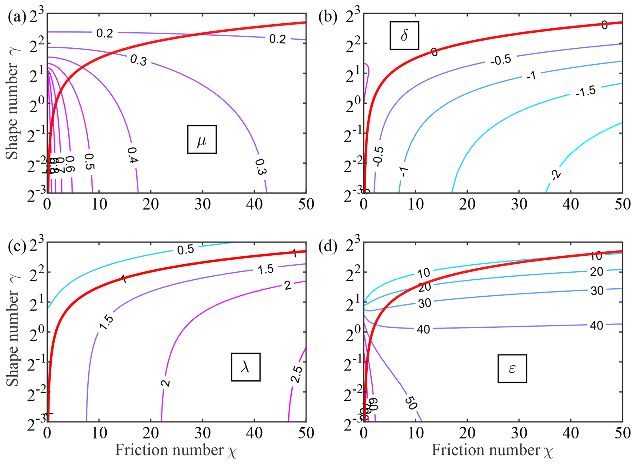
Figure 1 Contour plot of the dimensionless dependent parameters (a: μ; b: δ; c: λ; d: ε) as a function of estuary shape number γ and friction number χ obtained with a linear model (Cai et al., 2012), in which thick red lines represent the ideal estuary, where δ=0, λ=1, $\mathit{\mu }=\mathrm{1}/\sqrt{{\mathit{\gamma }}^{\mathrm{2}}+\mathrm{1}}$ and $\tan \left(\mathit{\epsilon }\right)=\mathrm{1}/\mathit{\gamma }$.

It is worth considering the solution in the special case of an ideal estuary (with no damping or amplification, δ=0) since natural estuarine systems tend to reach an equilibrium state of ideal estuaries. By imposing δ=0 in the set of Eqs. (16)–(19), one can easily obtain

$$\begin{array}{}\text{(23)}& \mathit{\delta }=\mathrm{0},\mathit{\lambda }=\mathrm{1},\mathit{\mu }={\displaystyle \frac{\mathrm{1}}{\sqrt{{\mathit{\gamma }}^{\mathrm{2}}}+\mathrm{1}}},\tan \left(\mathit{\epsilon }\right)={\displaystyle \frac{\mathrm{1}}{\mathit{\gamma }}}.\end{array}$$

Figure 1 shows the variation of the four dimensionless parameters as a function of γ and χ obtained by solving Eqs. (16)–(19). The thick red lines indicate the values for the special case of an ideal estuary, which follows directly from Eq. (23).

It is important to note that the analytical solutions of the linear model are local because they depend only on local (fixed position) quantities (i.e. the local tidal-amplitude-to-depth ratio ζ, the local estuary shape number γ and the local friction number χ). To follow along-channel variations of these local variables, a multi-reach approach (subdividing the whole estuary into short reaches) has been used, in which the damping number δ is integrated in short reaches over which the estuary shape number γ and the friction number χ are assumed to be constant. This is done by using simple explicit integration of the linear differential equation (Savenije et al., 2008):

$$\begin{array}{}\text{(24)}& {\mathit{\eta }}_{\mathrm{1}}={\mathit{\eta }}_{\mathrm{0}}+{\displaystyle \frac{\mathrm{d}\mathit{\eta }}{\mathrm{d}x}}\mathrm{\Delta }x={\mathit{\eta }}_{\mathrm{0}}+{\displaystyle \frac{\mathit{\delta }{\mathit{\eta }}_{\mathrm{0}}\mathit{\omega }\mathrm{\Delta }x}{c_{\mathrm{0}}}},\end{array}$$

where η₀ is the tidal amplitude at the origin of the axis for every short reach, while η₁ is the tidal amplitude at a distance Δx (e.g. 1 km) upstream.

2.2 Estimation of the tidally averaged depth

To address directly the correspondence between tidal dynamics and morphology, the celerity equation (Eq. 19) proposed by Savenije and Veling (2005) is considered. This analytical relationship is an extension of the classical celerity equation for a progressive wave in a frictionless prismatic channel and depicts the along-channel wave celerity ($\mathit{\lambda }=c_{\mathrm{0}}/c$) as a function of the tidal damping (δ) and estuary shape number (γ), hence accounting implicitly for the water depth (see Eq. 9). Figure 2 shows the analytically computed λ² over a wide range of values of δ, from −3 to 1, and γ, from 0 to 4, directly from Eq. (19). It can be clearly seen from Fig. 2 that there exist two distinct types of estuaries characterized by the threshold of δ=0. For positive values of δ (amplified estuary), λ<1, since the actual wave celerity c is larger than the classical one c₀, while it is the opposite (λ>1) for negative values of δ (damped estuary). The underlying mechanism lies in the imbalance between channel convergence and bottom friction (i.e. stronger impact of convergence than friction in the case of amplification, and the opposite in the case of damping). Without damping or amplification (λ=1, indicating balance between convergence and friction), the estuary corresponds to an ideal estuary, where the wave celerity equals c₀. Interestingly, according to Eq. (19), for an amplified estuary (δ>0), the actual wave celerity c could be equal to c₀ for the special case of γ=δ, which is due to the balance between channel convergence and acceleration effects (Jay, 1991).

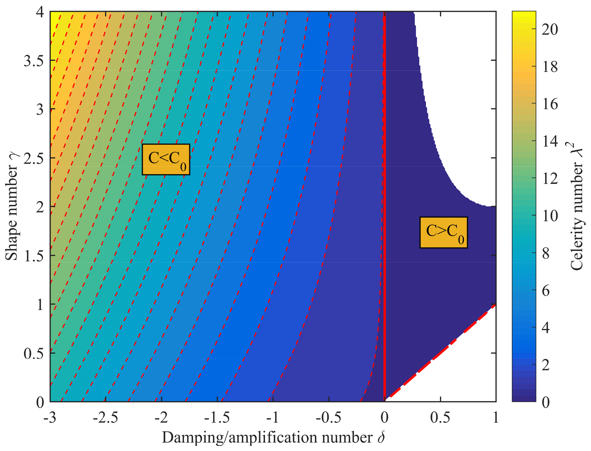
Figure 2 Contour plot of the celerity number λ² as a function of estuary shape number γ and damping/amplification number δ obtained from Eq. (19). The thick red line indicates the case of an ideal estuary (δ=0, c=c₀).

Estimation of the tidally averaged depth $\stackrel{\mathrm{‾}}{h}$ can be derived analytically by rewriting Eq. (19) in terms of the width convergence length b, wave celerity c and tidal damping (or amplification) rate δ_H, which leads to (see details in Appendix B)

$$\begin{array}{}\text{(25)}& \stackrel{\mathrm{‾}}{h}={\displaystyle \frac{r_{\mathrm{S}}b{c}^{\mathrm{2}}{\mathit{\omega }}^{\mathrm{2}}}{g\left({\mathit{\delta }}_H{c}^{\mathrm{2}}-{\mathit{\delta }}_H^{\mathrm{2}}{c}^{\mathrm{2}}b+b{\mathit{\omega }}^{\mathrm{2}}\right)}}.\end{array}$$

Here, the wave celerity c and the tidal damping (or amplification) rate δ_H can be estimated for a reach of Δx:

$$\begin{array}{}\text{(26)}& {\displaystyle }& {\displaystyle }c={\displaystyle \frac{c_{\mathrm{HW}}+c_{\mathrm{LW}}}{\mathrm{2}}}={\displaystyle \frac{\mathrm{\Delta }x}{\mathrm{2}}}\left({\displaystyle \frac{\mathrm{1}}{\mathrm{\Delta }{t}_{\mathrm{HW}}}}+{\displaystyle \frac{\mathrm{1}}{\mathrm{\Delta }{t}_{\mathrm{LW}}}}\right),\text{(27)}& {\displaystyle }& {\displaystyle }{\mathit{\delta }}_H={\displaystyle \frac{\mathrm{1}}{\left({\mathit{\eta }}_{\mathrm{1}}+{\mathit{\eta }}_{\mathrm{2}}\right)/\mathrm{2}}}{\displaystyle \frac{{\mathit{\eta }}_{\mathrm{2}}-{\mathit{\eta }}_{\mathrm{1}}}{\mathrm{\Delta }x}},\end{array}$$

where c_HW and c_LW are the wave celerity for HW and LW, respectively; Δt_HW and Δt_HW are the corresponding travelling times over the reach; η₁ is the tidal amplitude in the seaward part; and η₂ is the tidal amplitude Δx upstream. The wave celerity c can also be estimated through harmonic analysis. In this case, Eq. (26) can be rewritten as

$$\begin{array}{}\text{(28)}& c={\displaystyle \frac{\mathrm{\Delta }x}{\left({\mathit{\varphi }}_{Z_{\mathrm{2}}}-{\mathit{\varphi }}_{Z_{\mathrm{1}}}\right)T/\mathrm{360}}},\end{array}$$

where ${\mathit{\varphi }}_{Z_{\mathrm{1}}}$ is the phase of elevation at the seaward station, while ${\mathit{\varphi }}_{Z_{\mathrm{2}}}$ is the corresponding values at Δx upstream. As illustrated in the next section, these parameters can be easily obtained from tidal gauge observations, providing a simple means to quickly assess the mean water depth with Eq. (25).

In the inverse analytical model, it should be noted that the estuary is regarded as an ensemble system characterized by a spatially averaged water depth and a specific width convergence length. Based on the analytical expression of tidally averaged depth (Eq. 25), the variations of depth with two variables (i.e. the wave celerity and the tidal damping or amplification rate) can be further explored by using the following derivatives:

$$\begin{array}{}\text{(29)}& {\displaystyle }& {\displaystyle \frac{\partial \stackrel{\mathrm{‾}}{h}}{\partial c}}={\displaystyle \frac{\mathrm{2}{r}_{\mathrm{S}}{b}^{\mathrm{2}}c{\mathit{\omega }}^{\mathrm{4}}}{g{\left({\mathit{\delta }}_H{c}^{\mathrm{2}}-{\mathit{\delta }}_H^{\mathrm{2}}{c}^{\mathrm{2}}b+b{\mathit{\omega }}^{\mathrm{2}}\right)}^{\mathrm{2}}}},\text{(30)}& {\displaystyle }& {\displaystyle \frac{\partial \stackrel{\mathrm{‾}}{h}}{\partial {\mathit{\delta }}_H}}={\displaystyle \frac{r_{\mathrm{S}}b{c}^{\mathrm{4}}\left(\mathrm{2}{\mathit{\delta }}_{H}b-\mathrm{1}\right)}{g{\left({\mathit{\delta }}_H{c}^{\mathrm{2}}-{\mathit{\delta }}_H^{\mathrm{2}}{c}^{\mathrm{2}}b+b{\mathit{\omega }}^{\mathrm{2}}\right)}^{\mathrm{2}}}}.\end{array}$$

Figure 3 illustrates the analytically computed depth with Eq. (25) as a function of the wave celerity c and tidal damping (or amplification) rate δ_H for a constant width convergence length b=200 km and storage width ratio r_S=1. It can be seen that the depth $\stackrel{\mathrm{‾}}{h}$ tends to increase with the celerity c since the value of $\partial \stackrel{\mathrm{‾}}{h}/\partial c$ is always positive (see Eq. 29). On the other hand, the depth $\stackrel{\mathrm{‾}}{h}$ decreases with the tidal damping (or amplification) rate δ_H until a minimum value is reached at a critical δ_H corresponding to the condition $\partial \stackrel{\mathrm{‾}}{h}/\partial {\mathit{\delta }}_H=\mathrm{0}$, i.e. ${\mathit{\delta }}_H=\mathrm{1}/\left(\mathrm{2}b\right)$ (see Eq. 30). A further increase of the δ_H yields an increase of $\stackrel{\mathrm{‾}}{h}$.

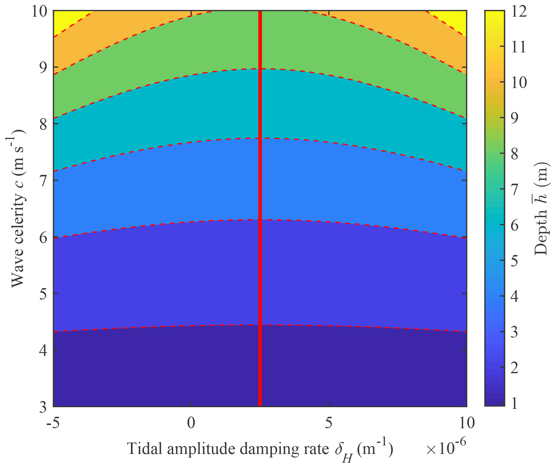
Figure 3 Contour plot of the estimated depth $\stackrel{\mathrm{‾}}{h}$ as a function of the wave celerity c and tidal damping (or amplification) rate δ_H obtained from Eq. (25). The drawn red line indicates the critical value of ${\mathit{\delta }}_H=\mathrm{1}/\left(\mathrm{2}b\right)$, corresponding to the minimum water depth for a given constant wave celerity.

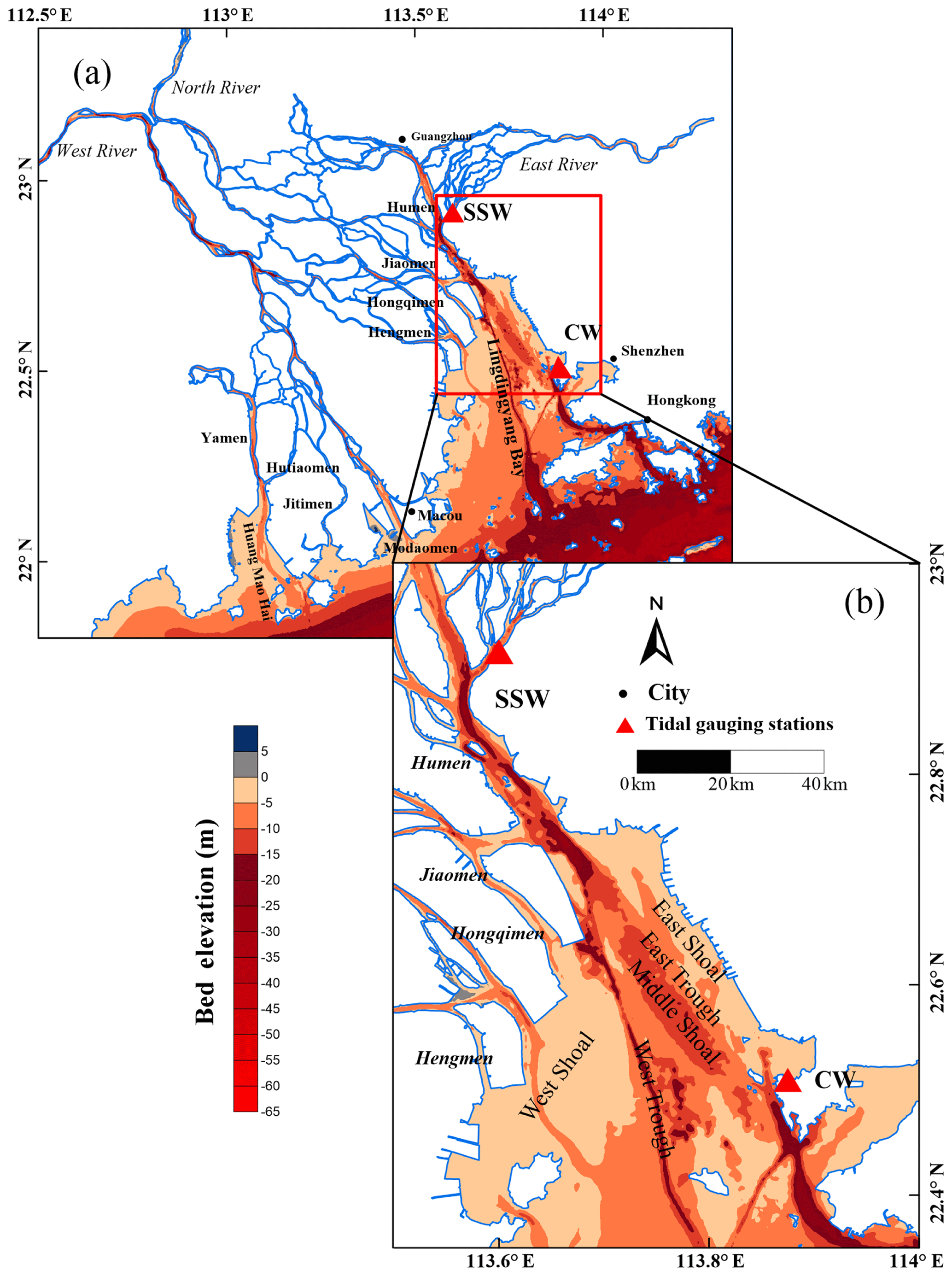
Figure 4 Sketch of Lingdingyang Bay (b) in the Pearl River Estuary (a).

3 Study area and datasets

3.1 Overview of Lingdingyang Bay

The Pearl River (Fig. 4a) delivered 2823×10⁸ m³ yr⁻¹ of freshwater and 72.4×10⁶ t yr⁻¹ of suspended sediment load (Liu et al., 2014) into the South China Sea during the period from the 1950s to the 2000s via eight outlets, i.e. four eastern outlets (Humen, Jiaomen, Hongqili and Hengmen) and four western outlets (Modaomen, Jitimen, Yamen and Hutiaomen). Lingdingyang Bay is the largest estuary of the Pearl River Estuary and mainly receives water and sediment inputs from the four eastern outlets (Fig. 4b). Lingdingyang Bay is a funnel-shaped subaqueous delta and has a complicated geomorphology pattern with two deep channels (i.e. east and west channels) between three shoals (i.e. east, middle and west shoals) (see Fig. 4b). The tide in Lingdingyang Bay mainly comes from the Pacific Ocean and has an irregular and semidiurnal character, with a mean tidal range between 1.0 and 1.7 m (Mao et al., 2004). Generally, tidal propagation in Lingdingyang Bay is affected by geometry (e.g. bank convergence), bottom topography and river discharge, among which the impact from river discharge is minor because the freshwater discharge is small compared to the amplitude of the tidal discharge. Hence, Lingdingyang Bay is a tide-dominated estuary. In response to the typical funnel shape topography, the mean tidal range is considerably amplified when a tidal wave propagates along Lingdingyang Bay, increasing from 1.1 m at Chiwan (denoted by CW hereafter) near the mouth to approximately 3.2 m at Sishengwei (denoted by SSW hereafter) near the head of the bay, located 58 km upstream. The tidal wave is continuously amplified until Huangpu gauging station (24 km upstream from CW) with a mean tidal range of approximately 3.6 m, after which it is damped until vanishing (Cai et al., 2019).

In recent decades, intensive human activities (e.g. land reclamation, channel dredging, sand excavation and dam constructions) have substantially disturbed the natural morphological evolution of Lingdingyang Bay. In particular, land reclamation was usually done in areas shallower than approximately 0.5 m; thus, nearly 200 km² of land was reclaimed during 1988–2008 (Wu et al., 2014). In addition, after the initial dredging of the west channel to produce a navigation channel with a target depth of 6.9 m in 1959, several other dredging operations were conducted to maintain a specific depth (e.g. 8.6 m in the 1980s). Since the 1990s, three stages of channel dredging were implemented in the west channel in 2001, 2007 and 2012, with target depths of −11.5, −13.0 and −17.0 m (relative to the datum of the lowest low water level, which is 1.7 m b.m.s.l. – below mean sea level), respectively (Li, 2008). Furthermore, sand excavation is conducted in Lingdingyang Bay. According to C. S. Wu et al. (2016), channel dredging and sand excavation caused local changes in the water depth of approximately 5 m yr⁻¹ between 2012 and 2013. Moreover, large amount of sediments were trapped due to the operation of upstream reservoirs, which also exerts substantial influence on the morphological evolution in Lingdingyang Bay. It was shown by C. S. Wu et al. (2016) that the volume of Lingdingyang Bay was dramatically increased during 2000–2010 owing to the combined influence of reduced sediment input, dredging and sand excavation.

3.2 Datasets

Bathymetric maps of Lingdingyang Bay with scales of 1:25 000, 1:50 000 and 1:75 000 (surveyed in 1965, 1974, 1989, 1998, 2009 and 2015) were provided by the Guangzhou Maritime Safety Administration and China People's Liberation Army Navy Command Assurance Department of Navigation. The water depths, isobaths and estuarine outlines on these maps were digitalized in order to generate a digital elevation model (DEM) used to analyse the morphological changes of Lingdingyang Bay over ∼50 years (from 1965 to 2015). Using the latitude and longitude information, they were then projected to UTM-WGS84 coordinates of China and interpolated to a 50 m×50 m grid DEM with kriging interpolation in ArcGIS, which was extensively applied to analyse the evolution of morphological changes (e.g. Brunier et al., 2014; Liu et al., 2019).

To explore the tidal hydrodynamics in Lingdingyang Bay, tidal water level records (see Fig. 5 for the records in January; the records in other months were not presented) for the periods with surveyed bathymetric maps were obtained from the Ministry of Water Resources of China (MWRC). These observations were taken at the CW and SSW gauging stations (see their locations in Fig. 4) and were used to have a first estimate of wave celerity (Eq. 26) and the tidal damping (or amplification) rate (Eq. 27) over the studied channel. From Fig. 5, we observe that the tide in Lingdingyang Bay is characterized by a semi-diurnal mixed tidal regime with apparent daily inequality in range and time between high and low waters. As the tide propagates from CW to SSW, the tidal range is amplified due to the strong channel convergence. The collected tidal water level records generally contained two high and two low water levels for each day. These data were then interpolated to 1 h intervals for harmonic analysis by using the shape-preserving piecewise cubic interpolation. The tidal water levels derived from such an interpolation method can well retain the power spectra of low-frequency bands and principal tides (e.g. M₂), while the high-frequency bands may not be entirely reproduced (see a similar result in Zhang et al., 2018, using a trigonometric interpolation method).

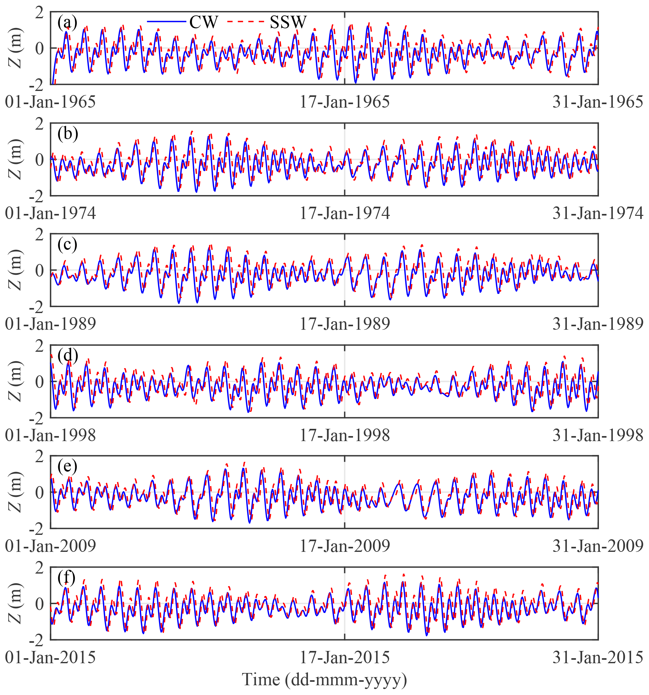
Figure 5 Observed water levels (relative to mean sea level) in January for different periods: (a) 1965, (b) 1974, (c) 1989, (d) 1998, (e) 2009 and (f) 2015.

Figure 6 shows the morphological changes in Lingdingyang Bay from 1965 to 2015. From 1965 to 1974, an area of 36.3 km² was reclaimed within the bay (see Table 1), extending the coastline southward towards the open sea (see Fig. 6A1, A2 and B1) and reducing the surface water area by 36.3 km² (Table 1). The magnitude of bathymetric changes was mainly less than 1 m in the bay (Fig. 6B1), with a general dominance of deposition. The mean water depth only decreased by 0.1 m (Table 1), corresponding to a water volume decrease of 2.0×10⁸ m³ during this period (Table 1). From 1974 to 1989, land reclamation was the most intensive, resulting in an increase in land area (and decrease in water area) of 129.2 km². During this period, significant deepening, ranging from 1 to 5 m, occurred in the west channel due to the dredging of the navigation channel. The mean water depth only increased by 0.1 m in Lingdingyang Bay. However, the water volume continued to decrease by 0.3×10⁸ m³ in relation to the decrease in water area. Since the 1990s, dredging for the maintenance of the navigation channel has intensified. From 1998 to 2015, land reclamation continued to increase the land area and decrease the water area in Lingdingyang Bay (Table 1). However, the mean water depth and water volume increased by 0.7 m and 5.1×10⁸ m³, respectively (Table 1), although Fig. 6A4 and A5 show that the west channel became narrower due to the expansion of the west shoal from 1998 to 2009. From 2009 to 2015, the area of the middle shoal was reduced, and pits up to ∼20 m deep occurred in its upper sector due to sand excavation (Fig. 6B5). It is evident that the morphological evolution in Lingdingyang Bay has been significantly altered by human activities since the 1990s.

Figure 6 Bathymetric maps of Lingdingyang Bay in 1965 (A1), 1974 (A2), 1989 (A3), 1998 (A4), 2009 (A5) and 2015 (A6) and its bathymetrical change rate during five time periods: 1965–1974 (B1), 1974–1989 (B2), 1989–1998 (B3), 1998–2009 (B4) and 2009–2015 (B5).

Table 1 Geometric characteristics observed in Lingdingyang Bay from 1965 to 2015.

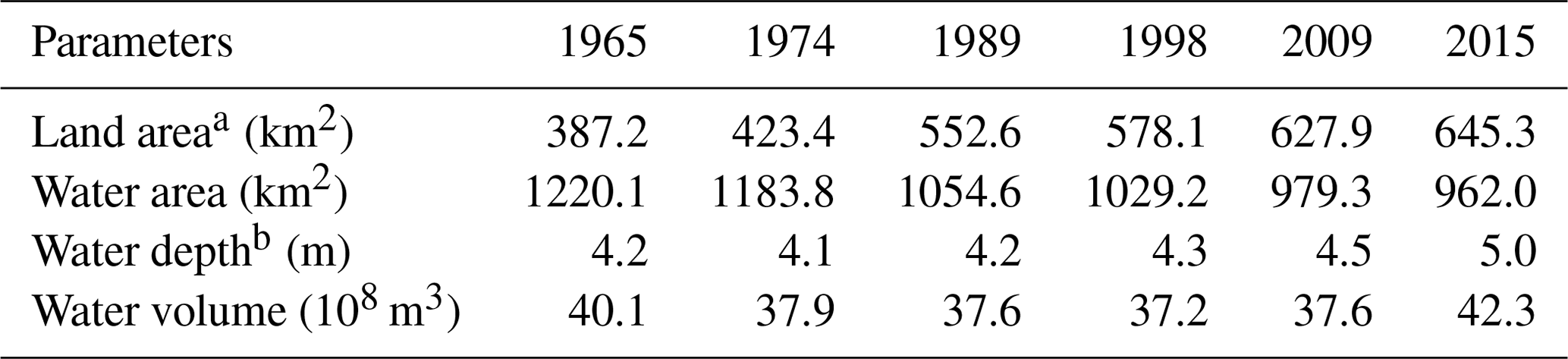
^a Difference between land areas in different years indicates the area of land reclaimed during this period. ^b Water depth was calculated below the datum of the lowest low water level, which is 1.7 m b.m.s.l.

4 Results

4.1 Variabilities of wave celerity and the tidal damping (or amplification) rate

In this paper, the observed wave celerity is derived from the travelling time of both high and low water levels (see Eq. 26), while the tidal damping (or amplification) rate is computed according to Eq. (27). To illustrate the spring–neap variabilities of tidal dynamics, Fig. 7 shows the observed c and δ_H as a function of the tidal amplitude at the estuary mouth η₀ (i.e. CW station) for different years. In general, we observe that both wave celerity and the damping (or amplification) rate decrease with increasing tidal amplitude at the estuary mouth with slightly different negative slopes (indicated by α and β representing the change rate of wave celerity and tidal damping or amplification rate with respect to the tidal amplitude, respectively), suggesting a more strongly amplified yet faster wave for the neap tide (smaller η₀, larger δ_H and c) than for the spring tide (larger η₀, smaller δ_H and c). Furthermore, we observe a clear pattern of increasing average wave celerity over the period between 1965 and 2015 (Fig. 7a–f), which corresponds to an increasing trend of the tidal amplification rate over the period. In addition, the spring–neap variability of tidal amplification is apparently large in 1965 and decreases until 2015.

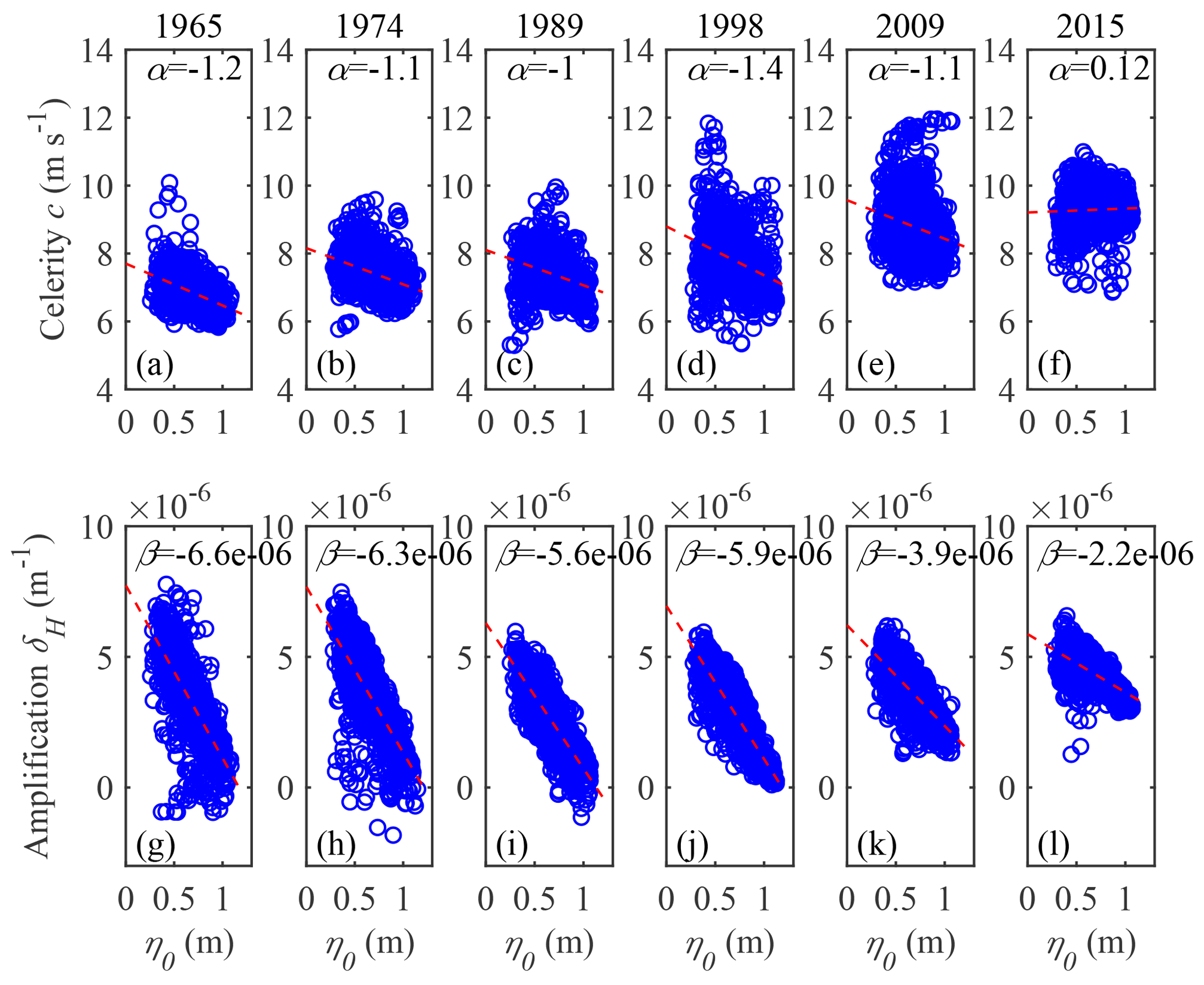
Figure 7 Estimations of wave celerity c and tidal damping (or amplification) rate δ_H as a function of the tidal amplitude at the CW station η₀ in Lingdingyang Bay, in which the red line represents the best-fit curve by linear regression with a gradient of α for celerity and β for tidal amplification.

Note that both the wave celerity and the tidal damping (or amplification) rate reflect the imbalance between channel convergence and bottom friction (Savenije and Veling, 2005). It is evident from the definition of the friction number χ (see Eq. 10) that effective bottom friction experienced for the spring tide is stronger than that for the neap tide due to a higher tidal-amplitude-to-depth ratio ζ during the spring tide. On the other hand, the estuary shape number γ and the tidally averaged depth $\stackrel{\mathrm{‾}}{h}$ are more or less the same for spring and neap tides. Hence, the tidal damping (or amplification) rate experienced by the estuary is larger for the neap tide than that for the spring tide.

To investigate the underlying mechanism of such a spring–neap variability of wave celerity, we further rewrite the celerity equation (Eq. 19) by substituting Eq. (12):

$$\begin{array}{}\text{(31)}& c={\displaystyle \frac{c_{\mathrm{0}}}{\sqrt{\mathrm{1}-\mathit{\delta }(\mathit{\gamma }-\mathit{\delta })}}}.\end{array}$$

It is evident from Eq. (31) that the wave celerity c increases with the tidal damping (or amplification) number δ for given constant values of γ and $\stackrel{\mathrm{‾}}{h}$. Hence, assuming a more or less constant tidally averaged depth over a spring–neap cycle, it is concluded that the wave celerity during the neap tide is generally faster than during the spring tide.

4.2 Performance of analytical model for reproducing the tidal hydrodynamics

Before an inverse analytical model can be used to predict the morphological changes in estuaries, it is required to calibrate and validate the model against observations well. Hence, the analytical model presented in Sect. 2.1 is used to reproduce the historic physical properties of the tidal wave (i.e. tidal damping or amplification rate and wave celerity) in Lingdingyang Bay. The estuarine system is subject to a harmonic tide at the estuary mouth (i.e. CW station). In order to calibrate and validate the analytical model, the tidal properties (including the tidal amplitude and phase) of the predominant M₂ tide at a monthly averaged scale were extracted by means of a classical harmonic analysis making use of the T_TIDE MATLAB Toolbox provided by Pawlowicz et al. (2002). Based on the collected topographic maps (see details in Sect. 3.2), the geometry of Lingdingyang Bay can be described by exponential functions (Eqs. 5 and 6) (Fig. 8), and the fitted geometric characteristics are given in Table 2. In order to account for the along-channel variations of the estuarine sections, we adopted a longitudinal variable depth along the channel. In Fig. 8, we also observe a sudden decrease in cross-sectional area near the Humen outlet, which is due to the strong width convergence towards the rock-bound gorges with a relatively greater water depth.

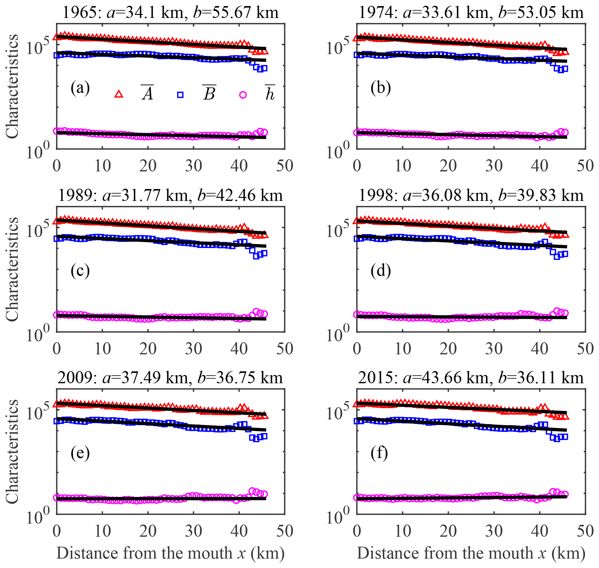
Figure 8 Longitudinal variations of the geometric characteristics (the tidally averaged cross-sectional area $\stackrel{\mathrm{‾}}{A}$, m²; width $\stackrel{\mathrm{‾}}{B}$, m; and depth $\stackrel{\mathrm{‾}}{h}$, m) of Lingdingyang Bay for different years (a: 1965; b: 1974; c: 1989; d: 1998; e: 2009; f: 2015), in which the black thin lines represent the best-fit curves according to the exponential functions (Eqs. 5 and 6).

Table 2 Geometric characteristics of Lingdingyang Bay.

^*: this indicates a spatially averaged value.

Table 3 Calibrated parameters used for the analytical model and the evaluation of its performance using RMSE.

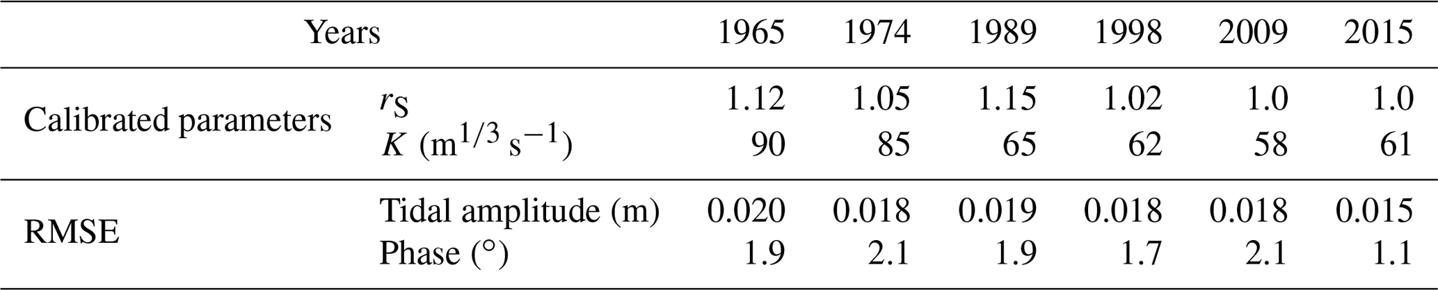
In Fig. 9, the analytically computed tidal amplitude η (see Eq. 24) and phase ϕ_Z (see Eq. 20) of the predominant M₂ tide at SSW (x=58 km) are compared with the observed values in Lingdingyang Bay for different years. We calibrated the analytical model by adjusting the Manning–Strickler friction coefficient K and the storage width ratio r_S, which are detailed in Table 3. In particular, the calibrated r_S is relatively sensitive to the variation in phase of the elevation. In addition, it is worth noting that in the analytical model the calibrated Manning–Stricker friction coefficient K should be regarded as an equivalent effective friction coefficient induced by the entire estuary, including the additional drag resistance due to bed forms, the influence of suspended sediments and the possible effect due to lateral storage areas (Cai et al., 2016). The model performance was evaluated by the root mean squared error (RMSE), where RMSE = 0 corresponds to perfect agreement. In general, the correspondence between analytical results and observations is good, both for the tidal amplitude (with RMSE ranging between 0.015 and 0.020 m) and the phases (with RMSE ranging between 1.1 and 2.1^∘), suggesting that the analytical model can reproduce the main tidal hydrodynamics in Lingdingyang Bay well. The calibrated friction coefficient K ranges between 58 and 90 m^1∕3 s⁻¹, with a minimum value occurring in 2009 (indicating relatively strong friction) and a maximum in 1965 (indicating relatively weak friction). On the other hand, the calibrated storage width ratio r_S is approximately unity (ranging between 1.0 and 1.15), which suggests a minor impact from the lateral storage areas on the evolution of tidal hydrodynamics.

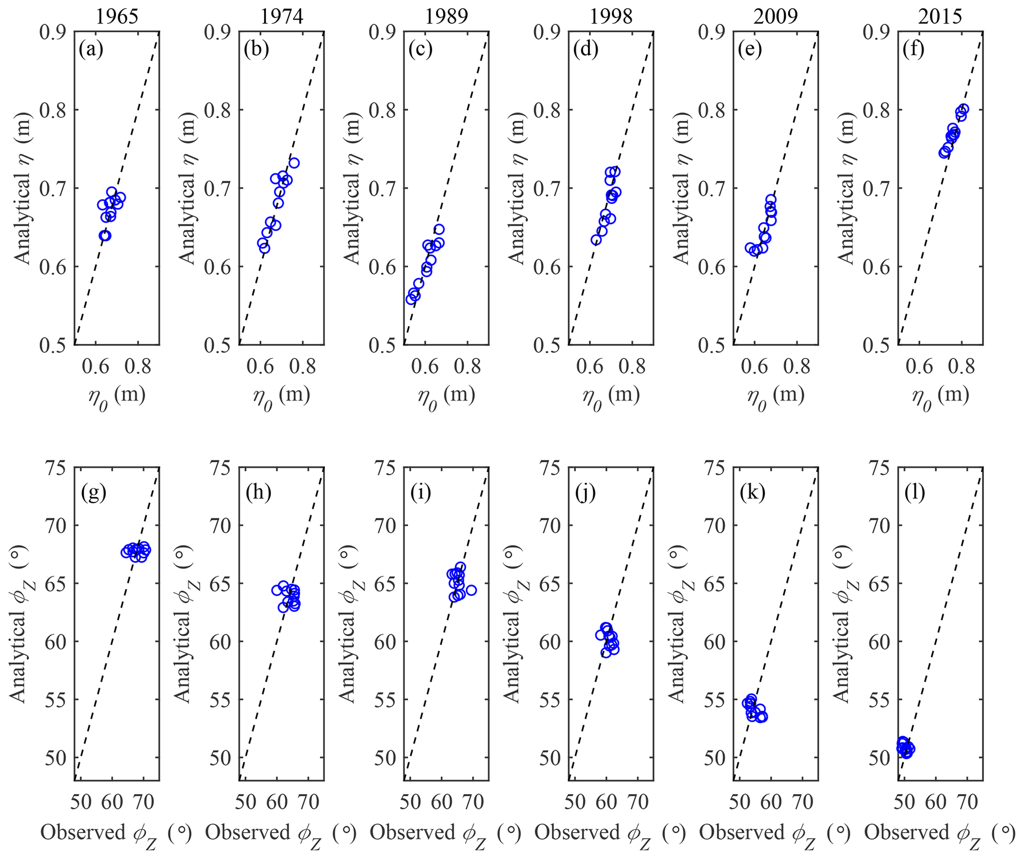
Figure 9 Comparison between analytically computed tidal amplitude η (a–f) and phase ϕ_Z (g–l) with observations in Lingdingyang Bay for different years. The dashed line represents the perfect match between analytical results and observations.

Subsequently, the analytically computed tidal characteristics of Lingdingyang Bay were used to describe how the tidal hydrodynamics are affected by the morphological evolution. In Fig. 10, the diagrams of the velocity number μ, damping number δ, celerity number γ and phase lag ε are shown together with the trajectory of their corresponding dimensionless parameters in Lingdingyang Bay. It is worth noting that the longitudinal estuary shape number γ decreased in 1965, 1974 and 1989 due to the shallowing of the estuary in the landward direction. Conversely, we observe an increased γ in 2009 and 2015, which is due to the increased depth in the channel (see Fig. 8). In these graphs, the longitudinal variations of the four dimensionless dynamics for different years are represented by different colours, where square symbols represent the initial position of CW station, while the circular symbols represent the position of SSW station. In Fig. 10, we can clearly see a transition in the hydrodynamics pattern during the studied period (1965–2015). Both the averaged values of the velocity number and damping/amplification number tend to decrease from 1965 to 1989, after which the values recover and approach the status of the 1960s. Figure 10c shows a similar picture for the celerity number, except that the values tend to increase from 1965 to 2015. In contrast, the longitudinal variation of phase lag displays a consistent decreasing tendency, which suggests that the tidal wave shows more of a standing-wave character with larger value of phase difference between velocity and elevation. Table 4 presents the spatially averaged values of the main dimensionless parameters over 1965–2015, where we see a clear transition pattern that occurs approximately around 1989. From the physical point of view, it can be seen that the tidal hydrodynamics become weak during the period of 1965–1989 (indicating lower values of μ and δ), after which the hydrodynamics becomes stronger in recent years (indicating larger values of μ and δ).

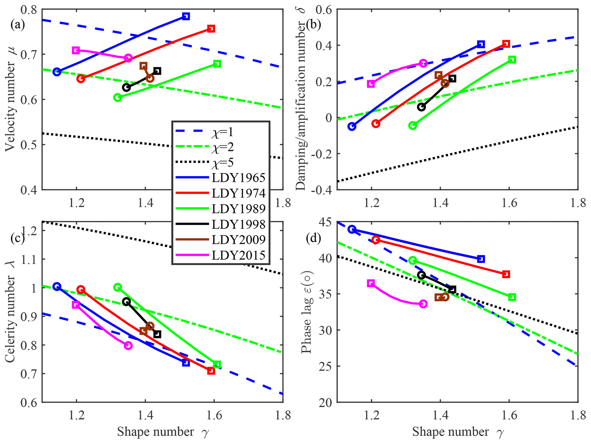
Figure 10 Trajectories of the main dimensionless parameters as a function of estuary shape number γ in Lingdingyang Bay (0–58 km) in (a) velocity number diagram, (b) damping/amplification number diagram, (c) celerity number diagram and (d) phase lag diagram. The square symbols indicate the initial position at CW station, while the circular symbols represent the final position at CW station. The background shows the lines of the hydrodynamics model with different values of the friction number χ.

Table 4 Spatially averaged dimensionless parameters in Lingdingyang Bay (0–58 km).

4.3 Estimation of the tidally averaged depth

The successful reproduction of tidal hydrodynamics using an analytical model suggests a close relationship between tidal damping (or amplification) and wave celerity, which can be described by the celerity equation (Eq. 19). Thus, it is possible to develop an inverse analytical model to estimate the tidally averaged depth $\stackrel{\mathrm{‾}}{h}$ for given observed wave celerity and the tidal damping (or amplification) rate from observed water levels, as presented in Sect. 2.2. In this case, we assume a constant depth; hence, the width convergence length equals the cross-sectional area length, i.e. a=b.

We adopted the width convergence length from topographic maps and estimated wave celerity and tidal damping (or amplification) from the observed water levels. Combining these parameters with the calibrated storage width ratio r_S (see Table 3), Eq. (25) can be used for a first estimate of the tidally averaged depth. Figure 11 shows the observed wave celerity and tidal damping (or amplification) together with the estimated tidally averaged depth and tidal amplitude at the CW station over the studied period. The monthly variation in estimated depth is mainly due to the change in mean sea level. In particular, we see a very similar variability of the derived depth to that of the wave celerity, which suggests a stronger influence of wave celerity when compared with the tidal amplification in Lingdingyang Bay.

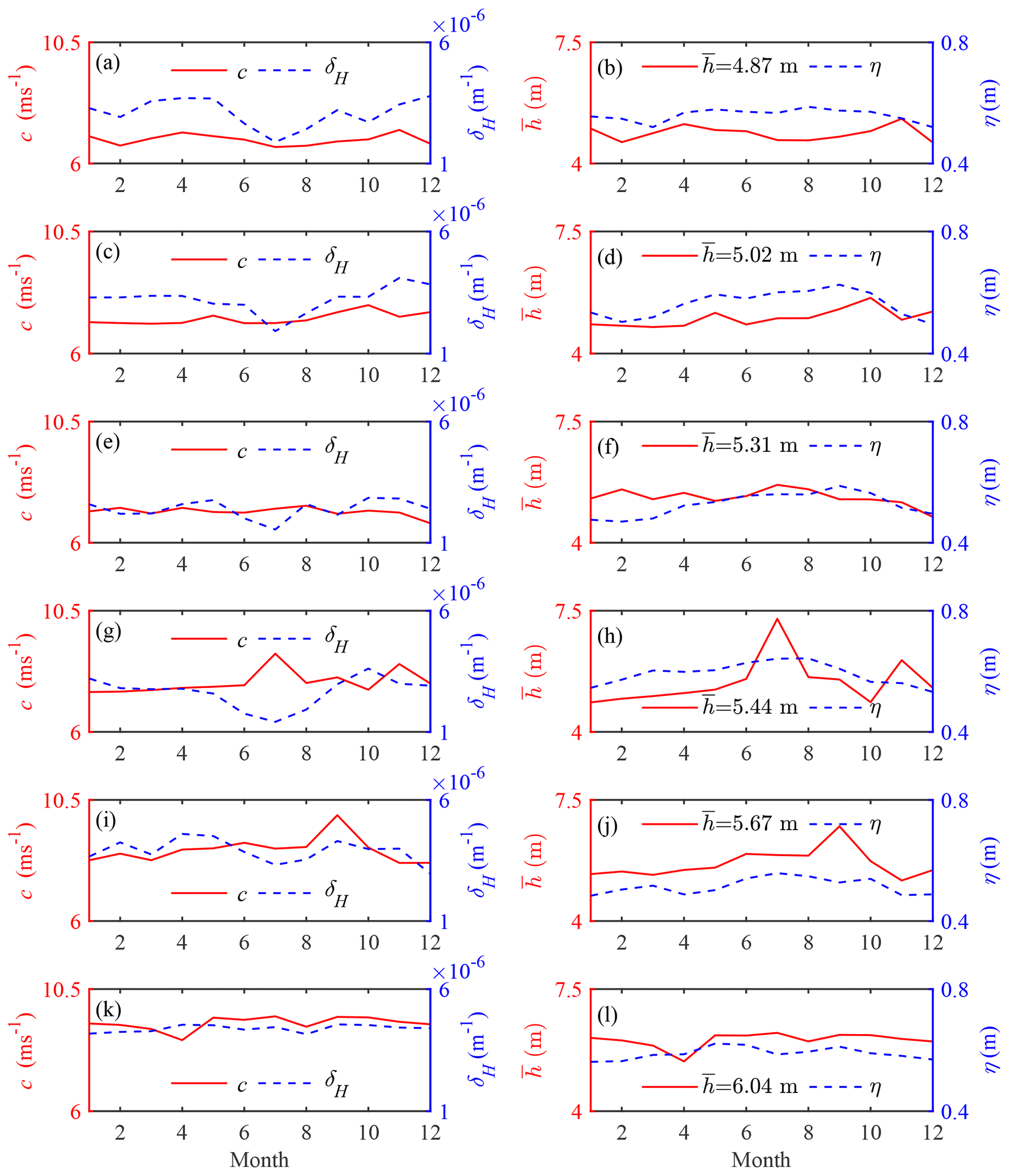
Figure 11 Estimation of the tidally averaged depth $\stackrel{\mathrm{‾}}{h}$ (b, d, f, h, j, l together with the tidal amplitude at the CW station η) using observed wave celerity c and tidal damping (or amplification) rate δ_H (a, c, e, g, i, k) for different years: 1965 (a, b), 1974 (c, d), 1989 (e, f), 1998 (g, h), 2009 (i, j) and 2015 (k, l).

Figure 12 shows the analytically computed tidally averaged depth and water volume at an annual scale in Lingdingyang Bay in different years. Note that in Fig. 12 the annual mean storage width ratio r_S and water area of Lingdingyang Bay were obtained by means of the shape-preserving piecewise cubic interpolation based on the calibrated and observed values, respectively. Here, the observed depth and water volume refer to the values relative to mean sea level, since the analytical model is derived based on a tidally averaged scale. For both geometric characteristics, the agreement with observations is reasonably good, with a RMSE of 0.068 m and 0.61×10⁸ m³, respectively. This suggests that the proposed method can be a useful tool for obtaining a first estimate of the morphological evolution in terms of depth and volume.

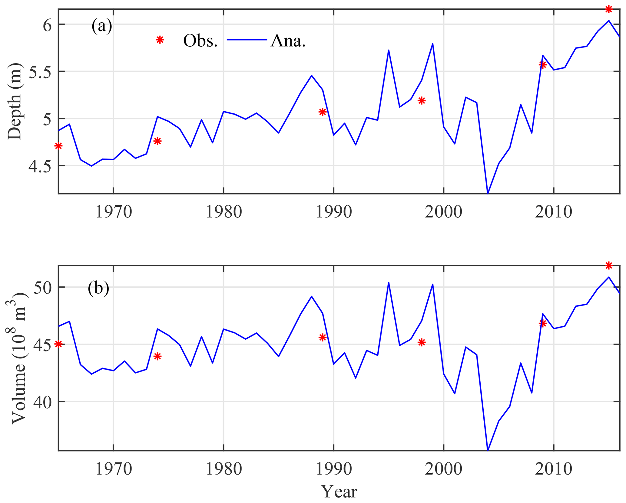
Figure 12 Comparison between analytically computed tidally averaged depth (a) and volume (b) with observations in Lingdingyang Bay.

5 Discussions

5.1 Influence of the morphological evolution on tidal hydrodynamics

Lingdingyang Bay is a typical funnel-shaped estuary, where the tidal dynamics are one of the main factors maintaining the stability state of estuarine morphology. Generally, the tides in the Pearl River Estuary are influenced by the geometry (i.e. cross-sectional variation) and river discharge (Zhang et al., 2010). The water discharge has shown insignificant change since the 1950s (Liu et al., 2017). Therefore, morphological changes became the main factors influencing the tidal dynamics of Lingdingyang Bay. Due to land reclamation, the water area and water volume of Lingdingyang Bay decreased from 1965 to 1974. Since the 1980s, channel dredging was conducted in the west channel (i.e. Lingding Channel) (C. S. Wu et al., 2016), and the west channel became deeper from 1974 to 1989 (Fig. 5B2). Therefore, although land area in Lingdingyang Bay increased by 30.5 % from 1974 to 1989, water volume only decreased by 0.8 %, and the mean water depth increased by 0.1 m (Table 1). In addition, since 1989, the mean water depth has increased significantly because of intensive channel dredging and reduced sediment inputs (due to reservoir operation in the Pearl River basin) in Lingdingyang Bay. Hence, it seems that the morphological evolution pattern of Lingdingyang Bay has changed since 1989. Correspondingly, temporal changes in the tidal dynamics of Lingdingyang Bay show that the tidal dynamics pattern has also changed since 1989 (see Figs. 7, 9 and 10 and Table 4).

To better understand the response of the morphological evolution to tidal dynamics, we rewrite the equilibrium depth h_I (subscript “I” indicates ideal estuary) through Eq. (18) for the case of an ideal estuary, where δ=0:

$$\begin{array}{}\text{(32)}& h_{\mathrm{I}}={\left({\displaystyle \frac{\mathrm{8}}{\mathrm{3}\mathit{\pi }{K}^{\mathrm{2}}}}\mathit{\upsilon }b\sqrt{g}\right)}^{\mathrm{6}/\mathrm{11}}.\end{array}$$

This shows that the equilibrium depth h_I is inversely proportional to the Manning–Strickler friction coefficient K to the power of 12∕11, while it is proportional to the velocity amplitude υ to the power of 6∕11. If we assume a more or less constant width convergence length, then the response of the morphological evolution can be inferred from the combined impacts from the Manning–Strickler friction coefficient (representing the bottom friction) and velocity amplitude (representing the tidal dynamics). Specifically, we observed a decreasing trend of calibrated K during 1965–1989, while there was an increasing trend during 1989–2015 (see Table 3). This suggests that the tidally averaged depth tends to increase before the 1990s, after which it would decrease again. However, we actually observed a consistent increase in water depth over the studied period, which has to do with the alteration of the tidal dynamics, especially due to the velocity amplitude. In Table 4, it can be seen that the dimensionless velocity number μ decreased from 1965 to 1989 (indicating a decreasing trend of water depth), after which it increased until 2015 (indicating an increasing trend of water depth). Hence, for the period of 1965–1989, the potential impact from bottom friction on morphological evolution dominated over the alteration of tidal dynamics. In contrast, the observed channel deepening in the following decades is mainly controlled by the reinforced tidal dynamics that has dominated over the bottom friction.

5.2 Model limitations

It should be noted that several assumptions are made in order to derive the analytical solutions for tidal hydrodynamics. The fundamental assumption is that the tidal-amplitude-to-depth ratio and the Froude number are considerably lower than unity so that the linearized Saint-Venant equations can be used for the derivations. A second fundamental assumption is that both the cross-sectional area and width can be described by exponential functions, following Eqs. (5) and (6), as is the case for most alluvial estuaries. We also assume that the cross section is mostly rectangular, with a possible impact from the lateral storage area described by the storage width ratio r_S. In this study, the r_S values were obtained by calibration against the extracting harmonic constants for given geometries observed in Lingdingyang Bay. For a fully predictive model, additional satellite maps (such as archived Landsat MSS/TM data, http://glovis.usgs.gov/, last access: 10 December 2019) at different periods (i.e. the spring tide and moderate tide) are required to help define the intertidal zone (and hence the r_S value). In addition, we neglect the influence of river discharge on tidal dynamics, which is not such a restriction in the downstream part of alluvial estuaries where the river flow velocity is small compared to the tidal velocity. It was shown that the tidally averaged depth varies due to the non-linear residual friction effect (e.g. Cai et al., 2014). By using a harmonic solution, the residual water level slope along the channel is assumed to be null, which means that the model cannot reproduce the spring–neap change of the tidally averaged depth along the channel, although the depth is usually larger during the spring tide (and also during the flood season) than during the neap tide (and also during the dry season) in tide-dominated estuaries. Moreover, by adopting an analytical solution for tidal hydrodynamics in an infinitely long channel, the model excludes the impact of reflected waves from the closed end on tidal dynamics. Therefore, the proposed analytical approach is preferably applied to tidally dominated estuaries (or bays) free of tidal barriers or sluices at the upstream end, where the tide dominates over the river discharge.

6 Conclusions

In this paper, a novel approach for estimating the tidally averaged depth was proposed to understand the morphological evolution based on the observed water levels at two stations (at least) in estuaries. The linear analytical hydrodynamics model proposed by Cai et al. (2012) was used to explore the hydrodynamics changes in Lingdingyang Bay, where we observe an evident hydrodynamics pattern transition due to the substantial changes of morphology. The analytically computed tidal amplitude and phase are compared to the observations, and the correspondence is good, which suggests that the proposed model can be a useful method for analysing the changes of physical tidal properties along the channel. Conversely, for given observed tidal water levels, it is possible to have a first estimate of wave celerity and tidal damping (or amplification) rate, and subsequently the tidally averaged depth and other tidal properties (e.g. velocity amplitude and phase lag), by manipulating the set of Eqs. (16)–(19). Thus, the proposed method could be particularly useful in situations where there are not sufficient data (e.g. detailed navigational charts) available but a first estimate of estuary depth and water volume is required.

Appendix A: Scaling the governing equations

We introduce scaling in Eqs. (2) and (3), similar to that used by Savenije et al. (2008), to derive the dimensionless equations, with the asterisk superscript denoting dimensionless variables:

$$\begin{array}{}\text{(A1)}& \begin{array}{rl}& U^{*}=U/{\mathit{\upsilon }}_{\mathrm{0}},h^{*}=h/\stackrel{\mathrm{‾}}{h},Z^{*}=Z/{\mathit{\eta }}_{\mathrm{0}},x^{*}=x{\displaystyle \frac{\mathrm{2}\mathit{\pi }}{L}},\\ & t^{*}=t{\displaystyle \frac{\mathrm{2}\mathit{\pi }}{T}},\end{array}\end{array}$$

where η₀ and υ₀ are the tidal amplitude and velocity amplitude at the estuary mouth, L is the wavelength and T is the tidal period. Note that the scaling of tidal flow velocity and water level fluctuation are slightly different from the scaling used by Savenije et al. (2008) because they are scaled with the corresponding values at the estuary mouth. For an infinite-length estuary, the velocity amplitude and the tidal amplitude are proportional:

$$\begin{array}{}\text{(A2)}& {\displaystyle \frac{\mathrm{1}}{\mathit{\upsilon }}}{\displaystyle \frac{\partial \mathit{\upsilon }}{\partial x}}={\displaystyle \frac{\mathrm{1}}{\mathit{\eta }}}{\displaystyle \frac{\partial \mathit{\eta }}{\partial x}},\end{array}$$

which implies that the ratio of the velocity amplitude to the tidal amplitude is constant:

$$\begin{array}{}\text{(A3)}& {\displaystyle \frac{\mathit{\upsilon }}{\mathit{\eta }}}={\displaystyle \frac{{\mathit{\upsilon }}_{\mathrm{0}}}{{\mathit{\eta }}_{\mathrm{0}}}}.\end{array}$$

When the non-linear continuity term $U\partial Z/\partial x$ and the advective term $U\partial U/\partial x$ are neglected and the assumption of Eq. A3 is made, Eqs. (2) and (3) may then be rewritten as

$$\begin{array}{}\text{(A4)}& {\displaystyle }& {\displaystyle \frac{\partial Z^{*}}{\partial t^{*}}}+\left({\displaystyle \frac{\stackrel{\mathrm{‾}}{h}\mathit{\upsilon }T}{\mathit{\eta }L{r}_{\mathrm{S}}}}\right)h^{*}{\displaystyle \frac{\partial U^{*}}{\partial x^{*}}}-\left({\displaystyle \frac{\stackrel{\mathrm{‾}}{h}\mathit{\upsilon }T}{\mathrm{2}\mathit{\pi }\mathit{\eta }b{r}_{\mathrm{S}}}}\right)h^{*}{U}^{*}=\mathrm{0},\text{(A5)}& {\displaystyle }& {\displaystyle \frac{\partial U^{*}}{\partial t^{*}}}+\left({\displaystyle \frac{g\mathit{\eta }T}{\mathit{\upsilon }L}}\right){\displaystyle \frac{\partial Z^{*}}{\partial x^{*}}}+\left(r{\displaystyle \frac{T}{\mathrm{2}\mathit{\pi }\stackrel{\mathrm{‾}}{h}}}\right)U^{*}=\mathrm{0}.\end{array}$$

The real scales of velocity amplitude υ and wavelength L are scaled with the corresponding values for a frictionless tidal wave in a channel with zero convergence (U₀, L₀) as a reference:

$$\begin{array}{}\text{(A6)}& {\displaystyle }& {\displaystyle }\mathit{\upsilon }=U_{\mathrm{0}}\mathit{\mu },\text{(A7)}& {\displaystyle }& {\displaystyle }L=L_{\mathrm{0}}/\mathit{\lambda },\end{array}$$

where we introduce the unknown dimensionless velocity number μ and celerity number λ.

For the case of a frictionless estuary with zero convergence, the classical wave celerity c₀ is defined by Eq. (1), while the velocity amplitude U₀ and the wavelength L₀ are

$$\begin{array}{}\text{(A8)}& {\displaystyle }& {\displaystyle }{U}_{\mathrm{0}}=\mathit{\zeta }{c}_{\mathrm{0}}{r}_{\mathrm{S}},\text{(A9)}& {\displaystyle }& {\displaystyle }{L}_{\mathrm{0}}=c_{\mathrm{0}}T,\end{array}$$

where ζ represents the dimensionless tidal-amplitude-to-depth ratio (see Eq. 15).

Under the assumption that $h^{*}=\mathrm{1}$ (i.e. $h=\stackrel{\mathrm{‾}}{h}$) in the continuity equation (Eq. A4), the dimensionless equations (Eqs. A4 and A5) read

$$\begin{array}{}\text{(A10)}& {\displaystyle }& {\displaystyle \frac{\partial z^{*}}{\partial t^{*}}}+\mathit{\mu }\mathit{\lambda }{\displaystyle \frac{\partial U^{*}}{\partial x^{*}}}-\mathit{\mu }\mathit{\gamma }{U}^{*}=\mathrm{0},\text{(A11)}& {\displaystyle }& {\displaystyle \frac{\partial U^{*}}{\partial t^{*}}}+{\displaystyle \frac{\mathit{\lambda }}{\mathit{\mu }}}{\displaystyle \frac{\partial z^{*}}{\partial x^{*}}}+{\displaystyle \frac{\mathrm{8}}{\mathrm{3}\mathit{\pi }}}\mathit{\mu }\mathit{\chi }{U}^{*}=\mathrm{0},\end{array}$$

where the dimensionless parameters γ and χ have been introduced as the estuary shape number (Eq. 9) and the friction number (Eq. 10), respectively, while the corresponding definitions of the velocity number μ and the celerity number λ are defined in Eqs. (11) and (12), respectively.

Appendix B: Derivation of the tidally averaged water depth from an inverse analytical model

Introducing the dimensionless parameters (Eqs. 9, 12 and 13) into the celerity equation (Eq. 19) yields

$$\begin{array}{}\text{(B1)}& {\left({\displaystyle \frac{c_{\mathrm{0}}}{c}}\right)}^{\mathrm{2}}=\mathrm{1}-{\displaystyle \frac{\mathrm{1}}{\mathit{\eta }}}{\displaystyle \frac{\mathrm{d}\mathit{\eta }}{\mathrm{d}x}}{\displaystyle \frac{c_{\mathrm{0}}}{\mathit{\omega }}}\left({\displaystyle \frac{c_{\mathrm{0}}}{\mathit{\omega }b}}-{\displaystyle \frac{\mathrm{1}}{\mathit{\eta }}}{\displaystyle \frac{\mathrm{d}\mathit{\eta }}{\mathrm{d}x}}{\displaystyle \frac{c_{\mathrm{0}}}{\mathit{\omega }}}\right),\end{array}$$

where a has been replaced by b in the definition of γ (Eq. 9) due to the assumption of a horizontal bed.

Substituting the classical wave speed $c_{\mathrm{0}}=\sqrt{g\stackrel{\mathrm{‾}}{h}/r_{\mathrm{S}}}$ (Eq. 1) and the tidal damping rate δ_H (Eq. 27) into Eq. (B1), we end up with Eq. (25) in the main text.