Does the weighting of climate simulations result in a better quantification of hydrological impacts?

With the increase in the number of available global climate models (GCMs), pragmatic questions come up in using them to quantify climate change impacts on hydrology: is it necessary to unequally weight GCM outputs in the impact studies, and if so, how should they be weighted? Some weighting methods have been proposed based on the performances of GCM simulations with respect to reproducing the observed climate. However, the process from climate variables to hydrological responses is nonlinear, and thus the assigned weights based on performances of GCMs in climate simulations may not be correctly translated to hydrological responses. Assigning weights to GCM outputs based on their ability to represent hydrological simulations is more straightforward. Accordingly, the present study assigns weights to GCM simulations based on their ability to reproduce hydrological characteristics and investigates their influences on the quantification of hydrological impacts. Specifically, eight weighting schemes are used to determine the weights of GCM simulations based on streamflow series simulated by a lumped hydrological model using raw or bias-corrected GCM outputs. The impacts of weighting GCM simulations are investigated in terms of reproducing the observed hydrological regimes for the reference period (1970–1999) and quantifying the uncertainty of hydrological changes for the future period (2070–2099). The results show that when using raw GCM outputs to simulate streamflows, streamflow-based weights have a better performance in reproducing observed mean hydrograph than climate-variable-based weights. However, when bias correction is applied to GCM simulations before driving the hydrological model, the streamflow-based unequal weights do not bring significant differences in the multi-model ensemble mean and uncertainty of hydrological impacts, since bias-corrected climate simulations become rather close to observations. Thus, it is likely that using bias correction and equal weighting is viable and sufficient for hydrological impact studies.

1 Introduction

Multi-model ensembles (MMEs) consisting of climate simulations from multiple global climate models (GCMs) have been widely used to quantify future climate change impacts and the corresponding uncertainty (Wilby and Harris, 2006; IPCC, 2013; Chiew et al., 2009; Chen et al., 2011; Tebaldi and Knutti, 2007). The number of climate models has increased rapidly, resulting in the obviously growing size of MMEs. For example, the Coupled Model Intercomparison Project Phase 5 (CMIP5) archive contains 61 GCMs from 28 modeling institutes, with some GCMs providing multiple simulations (Taylor et al., 2012). Due to the lack of consensus on the proper way to combine simulations of an MME, the prevailing approach is the model democracy (“one model one vote”) for the sake of simplicity, where each member in an ensemble is considered to have equal ability in simulating historical and future climates. The model democracy method has been applied to many global and regional climate change impact studies (e.g., IPCC, 2014; Minville et al., 2008; Maurer, 2007). Although it has been reported that the equal average of an MME often outperforms any individual model in regards to the reproduction of the mean state of observed historical climate (Gleckler et al., 2008; Reichler and Kim, 2008), whether the equal weighting is a better strategy for hydrological impact studies remains to be investigated (Alder and Hostetler, 2019).

Several studies have raised concerns about the strategy of model democracy due to the following two reasons (Lorenz et al., 2018; Knutti et al., 2017; Cheng and AghaKouchak, 2015). First, GCM simulations in an ensemble do not have identical skills for representing historical climate observations. They may perform differently in simulating future climate. GCM performances may also vary by their variables and locations (Hidalgo and Alfaro, 2015; Abramowitz et al., 2019), which further challenges the rationality of model democracy in regional impact studies. Second, equal weights imply that the individual members in an ensemble are independent of each other. However, some climate models share common modules, parts of codes, parameterizations, and so on (Knutti et al., 2010; Sanderson et al., 2017). Some pairs of GCMs submitted to the CMIP5 database only differ in the spatial resolution (e.g., MPI-ESM-MR and MPI-ESM-LR; see Giorgetta et al., 2013). The replication or overlapping in these GCMs may lead to the interdependence of MMEs, resulting in common biases towards the replicating section and inflating confidence in the projection uncertainty (Sanderson et al., 2015; Jun et al., 2012).

With the intention of improving climate projections and reducing the uncertainty, some weighting approaches have been proposed to assign unequal weights to climate model simulations according to their performances with respect to reproducing some diagnostic metrics of historical climate observations (Murphy et al., 2004; Sanderson et al., 2017; Cheng and AghaKouchak, 2015). For example, Xu et al. (2010) apportioned weights for GCMs based on their biases to the observed data in terms of two diagnostic metrics (climatological mean and interannual variability) for producing probabilistic climate projections. Lorenz and Jacob (2010) used errors in the trends of temperature to evaluate climate projections and determine weights. Other criteria have also been introduced into model weighting as a complement to the performance criterion. Some examples are the convergence of climate projections for a future period (Giorgi and Mearns, 2002) and the interdependence among climate models (Sanderson et al., 2017).

Despite the different diagnostic metrics or definitions of model performances employed in these weighting methods, weights are commonly determined with respect to the ability of climate simulations to reproduce observed climate variables, such as temperature and precipitation (e.g., Chen et al., 2017; Wilby and Harris, 2006; Xu et al., 2010). However, for the impact studies, the relationship between climate variables and the impact variable is often not straightforward or explicit. In other words, the process from climate variables to their impacts may not be linear (Wang et al., 2018; Risbey and Entekhabi, 1996; Whitfield and Cannon, 2000). For example, Mpelasoka and Chiew (2009) reported that in Australia, a small change in annual precipitation can result in a change in annual runoff that is several times larger. Thus, the weights calculated in the climate field may not be effective in the impact field.

In addition, a number of climate variables may determine the climate change impacts on a single environmental sector. For example, the runoff generation in a watershed is usually determined by precipitation, temperature, and other climate variables. Thus, it is not an easy task to determine the relative importance of each climate variable in impact studies, which is the other challenge in combining sets of weights based on different climate variables into a single set of weights for impact simulations. Previous studies have usually assumed that all variables are equally important and had an equal weight assigned to each climate variable (Xu et al., 2010; Chen et al., 2017; Zhao, 2015). However, these climate variables are usually not equally important in the impact field. For example, precipitation may be more important than temperature for a rainfall-dominated watershed, but this could be different for a snowfall-dominated watershed. Thus, it may be more straightforward to calculate the weights for GCMs based on their ability to reproduce the single impact variable instead of multiple climate variables. Such a method would integrate the synthetic ability of GCMs in terms of simulating multiple climate variables to that of one impact variable. In addition, this method could also circumvent the previous problem of potential nonlinearity between climate variables and the impact variable.

Accordingly, the objectives of this study are to assign weights to GCM simulations according to their ability to represent hydrological observations and to assess the impacts of these weighting methods on the quantification of hydrological responses to climate change. The case study was conducted over two watersheds with different climatic and hydrological characteristics. Since both bias correction and model weighting are common procedures in regional and local impact studies, this study considers two experiments (raw and bias-corrected GCM outputs) to simulate streamflows and investigate the performances of weighting methods. Seven weighting methods were used to assign unequal weights for streamflows simulated by raw or bias-corrected GCMs. The impacts of unequal weights are then assessed and compared to the equal-weighting method in terms of multi-model ensemble mean and uncertainty related to the choice of a climate model.

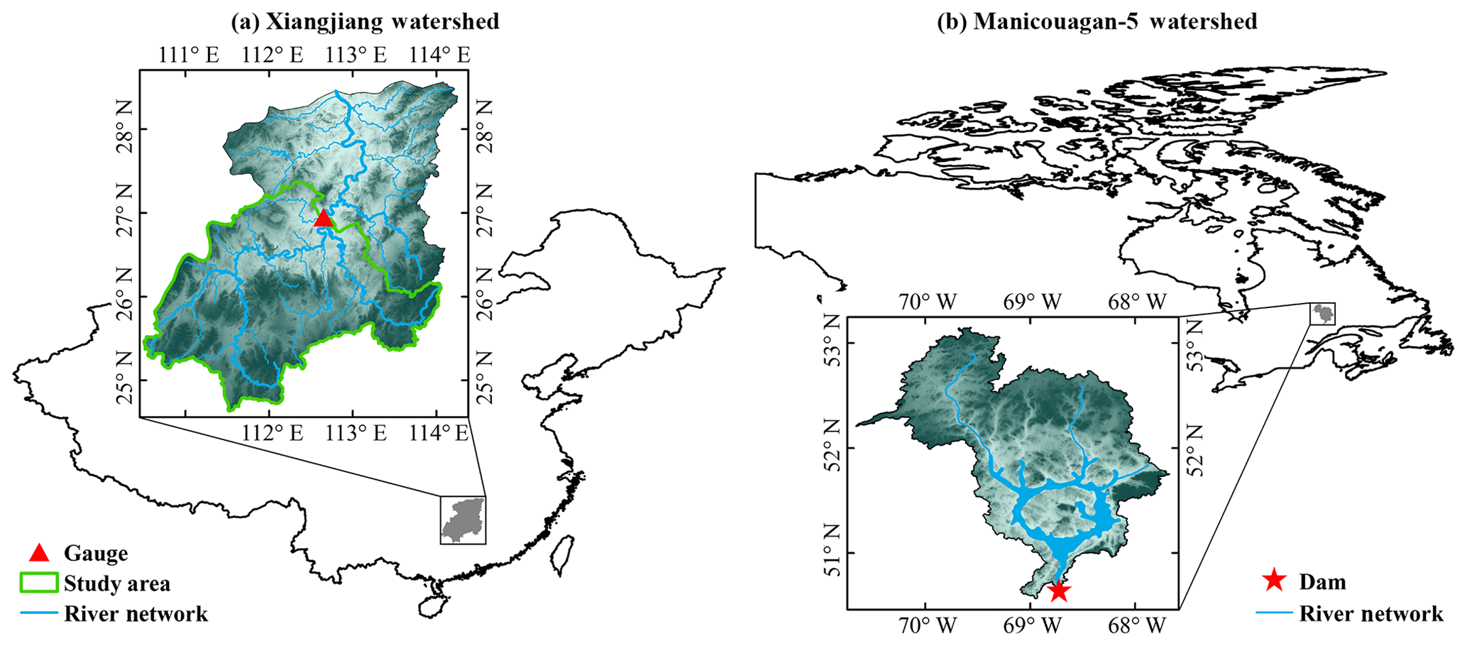
Figure 1 Locations of the (a) Xiangjiang and (b) Manicouagan-5 watersheds. (The study area in the Xiangjiang watershed is one of its sub-basins, shown here as the green boundary.)

2 Study area and data

2.1 Study area

This study was conducted over two watersheds with different climatic and hydrological characteristics: the rainfall-dominated Xiangjiang watershed and the snowfall-dominated Manicouagan-5 watershed (Fig. 1). The Xiang River is one of the largest tributaries of the Yangtze River in central–southern China, and its drainage area is about 94 660 km² (Fig. 1a). A catchment with a surface area of about 52 150 km² above the Hengyang gauged station was used in this study. The catchment is heavily influenced by the East Asian monsoon, which causes a humid subtropical climate with hot and wet summers and mild winters. The average temperature over the catchment is about 17 ^∘C, with the coldest month averaging at about 7 ^∘C. The average annual precipitation is about 1570 mm, of which 61 % falls in the wet season from April to August. The daily averaged streamflow at the Hengyang gauged station is around 1400 m³ s⁻¹. The annual average of summer peak streamflow is about 4420 m³ s⁻¹, which is mainly due to summer extreme rainfalls.

The Manicouagan-5 watershed, located in the center of the province of Quebec, Canada, is the largest sub-basin of the Manicouagan watershed (Fig. 1b). Its drainage area is about 24 610 km², most of which is covered by forest. The outlet of the Manicouagan-5 watershed is the Daniel-Johnson Dam. The Manicouagan-5 watershed has a continental subarctic climate characterized by long and cold winters. The average temperature over the watershed is about −3 ^∘C, with nearly half of the year having a daily temperature below 0 ^∘C. The average annual precipitation is about 912 mm. The average discharge at the outlet of the Manicouagan-5 watershed is about 530 m³ s⁻¹. Snowmelt contributes to the peak discharge during May, which has an annual average of about 2200 m³ s⁻¹.

2.2 Data

This study used daily maximum and minimum temperatures and precipitation from observation and GCM simulations for both watersheds. The observed meteorological data for the Xiangjiang watershed were collected from 97 precipitation gauges and 8 temperature gauges. Streamflow series were collected from the Hengyang gauged station. For the Manicougan-5 watershed, the observed meteorological data were extracted from the gridded dataset of Hutchinson et al. (2009), which is interpolated from daily station data using a thin-plate smoothing spline interpolation algorithm. Streamflow series were the inflows of the Daniel-Johnson Dam, which were calculated using mass balance calculations. All the observation data for both watersheds cover the historical reference period (1970–1999).

For the climate simulations, maximum and minimum temperatures and precipitation of 29 GCMs were extracted from the CMIP5 archive over both watersheds (Table 1). All simulations cover both the historical reference period (1970–1999) and the future projection period (2070–2099). One Representative Concentration Pathway (RCP8.5) was used in terms of climate projections in the future period. RCP8.5 was selected because it projects the most severe increase in greenhouse gas emissions among the four RCPs, and it is often used to design conservative mitigation and adaptation strategies (IPCC, 2014).

Table 1 Information about the 29 GCMs used.

3 Methodology

To begin the process of calculating the weights for each GCM simulation, the multi-model ensemble constructed by 29 GCMs was utilized to drive a calibrated hydrological model over the two watersheds. Two experiments were designed to generate the ensembles of streamflow simulations. The first experiment drives the hydrological model using raw GCM outputs with no bias correction, while the second drives the hydrological model using bias-corrected climate simulations. Although it is not common to use raw GCM simulations for hydrological impact studies, the rationale for using them in this study is to examine the impacts of bias correction on weighting GCMs. The bias correction may adjust the relative performances between climate simulations and thus affect the determination of the relative weight for each ensemble member. Based on the ensemble of hydrological simulations from GCM outputs, eight weighting methods were employed to determine the weights of each GCM and to combine ensemble members for the assessment of hydrological climate change impacts. More detailed information is given below.

3.1 Bias correction

Since the raw outputs of GCMs are often too coarse and biased to be directly input into hydrological models for impact studies, bias correction is commonly applied to GCM outputs prior to the runoff simulation (Wilby and Harris, 2006; Chen et al., 2011; Minville et al., 2008). A distribution-based bias-correction method, the daily bias-correction (DBC) method of Chen et al. (2013), was used in this study. DBC is the combination of the local intensity scaling (LOCI) method (Schmidli et al., 2006) and the daily translation (DT) method (Mpelasoka and Chiew, 2009). The LOCI method was used to adjust the wet-day frequency of climate-model-simulated precipitation. A threshold was determined for the reference period to ensure that the simulated precipitation occurrence is identical to the observed precipitation occurrence. The same threshold was then used to correct the wet-day frequency for the future period. The DT method was used to correct biases in the frequency distribution of simulated precipitation amounts and temperature separately. The frequency distribution was represented by 100 percentiles, ranging from the 1st to the 100th, and the correction factors were calculated for each percentile in the reference period. The same correction factors were then employed to correct the distributions for the future period. The use of distribution-based biases facilitates the use of different correction factors for different levels of precipitation. Some studies have shown the advantages of distribution-based bias correction over other correction methods in the assessment of hydrological impacts (Chen et al., 2013; Teutschbein and Seibert, 2012). Each variable was corrected independently, and inter-variable dependence was not considered in this study. Previous study has shown that the use of a more complicated method does not manifest much advantage over the use of the independent bias-correction method for these two watersheds (Chen et al., 2018).

3.2 Runoff simulation

The runoff was simulated using a lumped conceptual hydrological model, GR4J-6 (Arsenault et al., 2015), which couples a snow accumulation and melt module, CemaNeige, to a rainfall–runoff model, Génie Rural à 4 paramètres Journalier (GR4J). The CemaNeige model divides the precipitation into liquid and solid according to the daily temperature range and generates snowmelt depending on the thermal state and water equivalent of the snowpack (Valéry et al., 2014). CemaNeige has two free parameters: the melting rate and the thermal-state coefficient. The GR4J model consists of a production reservoir and a routing reservoir (Perrin et al., 2003). A portion of net rainfall (liquid precipitation with evaporation subtracted) goes into the production reservoir, whose leakage forms the effective rainfall when combined with the other proportion of net rainfall. The effective rainfall is then divided into two flow components. Ninety percent of the effective rainfall routes via a unit hydrograph and enters into the routing reservoir. The other 10 % generates the direct flow through the other unit hydrograph. There is groundwater exchange with neighboring catchments in the direct flow and the outflow nonlinearly generated by the routing reservoir. Four free parameters in GR4J must be calibrated: the maximum capacity of the production reservoir, the groundwater exchange coefficient, the 1 d ahead maximum capacity of the routing reservoir, and the time base of unit hydrograph. A brief flowchart of the GR4J-6 model is shown in the Supplement (Fig. S1).

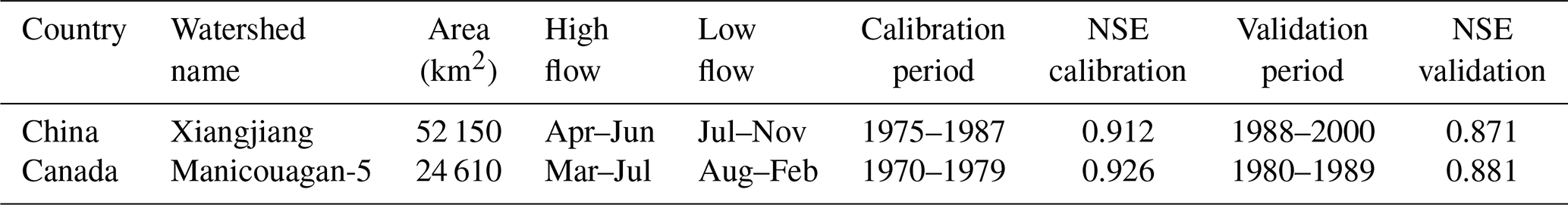
The time periods of the observed data used for hydrological model calibration and validation are presented in Table 2. The shuffled complex evolution optimization algorithm (Duan et al., 1992) was employed to optimize the parameters of GR4J-6 for both watersheds. The optimized parameters were chosen to maximize the Nash–Sutcliffe efficiency (NSE) criterion (Nash and Sutcliffe, 1970). The selected sets of parameters yield NSEs greater than 0.87 for both calibration and validation periods, indicating the reasonable performance of GR4J-6 and the high quality of the observed datasets for both watersheds.

Table 2 Nash–Sutcliffe efficiency (NSE) of the hydrological model in the calibration and validation periods.

3.3 Weighting methods

Raw and bias-corrected climate simulations were input to the calibrated GR4J-6 model to generate raw and bias-corrected streamflow data series, respectively. Eight weighting methods were then employed to determine the weight of each hydrological simulation, including the equal-weighting method (model democracy) and seven unequal-weighting methods. All of the unequal-weighting methods are described in detail in the Supplement, so they are only briefly presented herein. Seven unequal-weighting methods consist of two multiple-criteria-based weighting methods and five performance-based weighting methods. The two multiple-criteria-based weighting methods are the reliability ensemble averaging (REA) method and the performance and interdependence skill (PI). The REA method of Giorgi and Mearns (2002) considers both the bias of a GCM to observation in the reference period (performance criterion) and its similarity to other GCMs in the future projection (convergence criterion). The PI method (Knutti et al., 2017; Sanderson et al., 2017) weights an ensemble member according to its bias to historical observation (performance criterion) and its distance to other ensemble members in the reference period (interdependence criterion). The biases and distances in the REA and PI methods were calculated based on the diagnostic metric of the climatological mean of streamflow.

The five performance-based weighting methods are the climate prediction index (CPI), upgraded reliability ensemble averaging (UREA), the skill score of the representation of the annual cycle (RAC), Bayesian model averaging (BMA), and the evaluation of the probability density function (PDF). All of these methods only consider the differences of climate simulations to historical observation, but they differ in the metrics or algorithms used to determine weights. The CPI assigns weights based on the biases in the climatological mean and assumes that the simulated climatological mean follows a Gaussian distribution (Murphy et al., 2004). UREA considers biases in both the climatological mean and the interannual variance to determine weights (Xu et al., 2010). Both the RAC and BMA calculate weights based on monthly series. The RAC defines a skill score in simulating the annual cycle according to the relationship among the correlation coefficient, standard deviations, and centered root-mean-square error (Taylor, 2001). BMA combines the results of multiple models through the Bayesian theory (Duan et al., 2007; Raftery et al., 2005; Min et al., 2007). The PDF determines weights according to the overlapping area of the probability density function between daily simulations and observations (Perkins et al., 2007).

Using all eight methods, the weights were calculated for each of streamflow data series simulated by raw GCM outputs and bias-corrected outputs. For comparison, raw and bias-corrected temperature and precipitation series were also individually used to calculate climate-based weights using the above weighting methods.

3.4 Data analysis

The extent of inequality of each set of weights was first investigated by the entropy of weights (Déqué and Somot, 2010). The entropy of weights reflects the extent of how a weighting method discriminates the relative reliability between GCM simulations. Next, in order to investigate the impacts of weighting GCM simulations for hydrological impact studies, weights were used to combine the ensemble of hydrological simulations. The impacts of unequal weights were compared to the results obtained using the equal-weighting method. The comparison focuses on three aspects: (1) the simulation of reference and future hydrological regimes, (2) the bias of the multi-model ensemble mean during the reference period, and (3) the uncertainty of changes in hydrological indices between future and reference periods.

To be specific, for the entropy of weights (Eq. 1), it reaches a maximum value when the weights are equally distributed among ensemble members. A smaller entropy indicates a larger difference among the weights of ensemble members. Thus, the entropy reflects the extent of inequality for a set of weights:

$$\begin{array}{}\text{(1)}& E=-\sum _{i=\mathrm{1}}^N{w}_i\ln w_i,\end{array}$$

where w_i is the weight assigned to the ith ensemble member, and N is the total number of ensemble members.

Since weighting methods are usually proposed to reduce biases in the ensemble of climate simulations, the multi-model ensemble means determined by these weights were then evaluated in terms of the representation of observation during the reference period. The multi-year averages of three hydrological indices were calculated for each streamflow simulation: (1) annual streamflow, (2) peak streamflow, and (3) the center of timing of annual flow (t_CMD: the occurrence day of the midpoint of annual flow). Then, the multi-model mean indices were obtained based on the weights assigned to each simulation and compared to the indices of observation.

The influences of model weighting on the uncertainty of hydrological impacts related to the choice of GCMs were investigated through the changes in four hydrological indices between the reference and future periods: (1) mean annual streamflow, (2) mean streamflow during the high-flow period, (3) mean streamflow during the low-flow period, and (4) mean peak streamflow (the periods of high and low flow are shown in Table 2). The Monte Carlo approach was introduced to sample the uncertainty for unequally weighted ensembles (Wilby and Harris, 2006; Chen et al., 2017). The hydrological indices were randomly sampled 1000 times based on the calculated weights. For example, if a climate model simulation is assigned a weight of 0.2, the hydrological index simulated by that climate simulation has a probability of 20 % of being chosen as the sample in each Monte Carlo experiment.

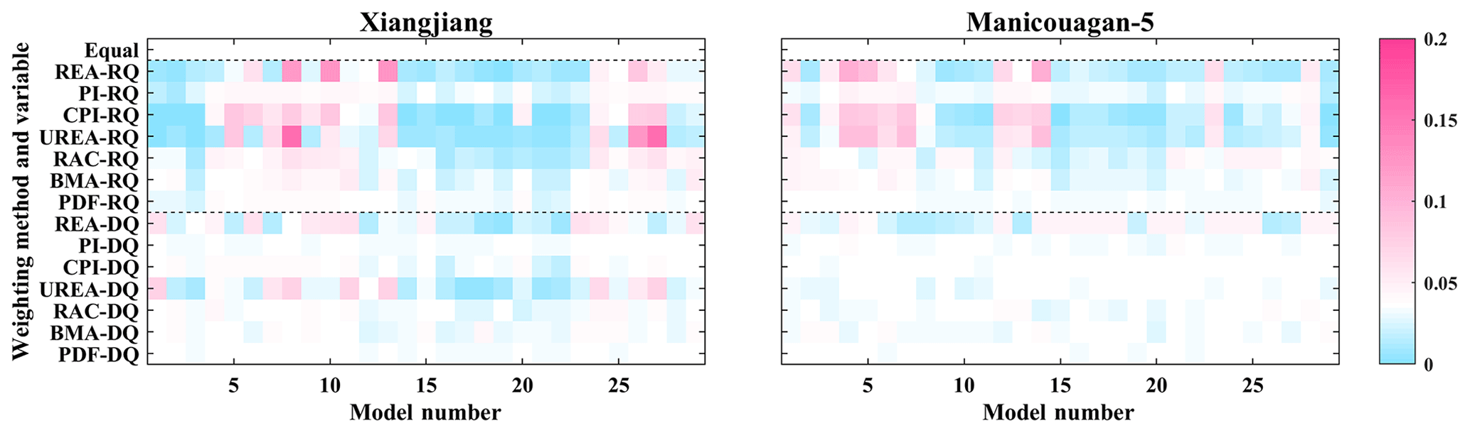
Figure 2 Weights assigned by equal weighting and seven unequal-weighting methods based on raw GCM-simulated streamflow (RQ) and bias-corrected GCM-simulated streamflow (DQ) for two watersheds. (Equal weight is presented in white; weights greater than equal are presented in red, and weights less than equal are represented in blue.)

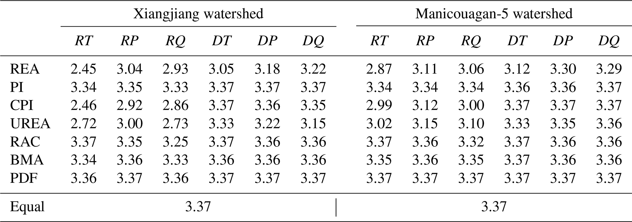
Table 3 The entropy of weights calculated by equal weighting and seven unequal-weighting methods based on raw GCM-simulated streamflow (RQ) and bias-corrected GCM-simulated streamflow (DQ) for two watersheds. The entropy of weights calculated based on raw and bias-corrected temperature (RT and DT) and precipitation (RP and DP) are also presented for comparison.

4 Results

4.1 Weights of GCMs

Figure 2 presents the weights calculated based on the streamflow series simulated by raw GCM outputs and bias-corrected outputs for eight (one equal and seven unequal) weighting methods over two watersheds. These results show the ability of different weighting methods to distinguish the performance or reliability of individual ensemble members. The entropy of weights was also calculated to quantify the extent of this disproportion for each set of weights (Table 3). Some weighting methods tend to aggressively discriminate the reliability of GCMs and assign differentiated weights to ensemble members, while other methods assign similar weights to each of them. Specifically, for the weights based on raw GCM-simulated streamflows, REA, UREA, and CPI produce the weights that most radically discriminate ensemble members among all eight weighting methods for both watersheds. The RAC method generates less differentiated unequal weights, followed by the BMA and PI methods, but weights assigned by the PDF method closely resemble the equal-weighting method. However, when weights are calculated based on bias-corrected GCM-simulated streamflows, the inequality of weights is reduced, and all the unequal-weighting methods receive a lower entropy of weights for both watersheds (Table 3). Most sets of these weights become similar to the equal-weighting method, with the exception of REA and UREA for the Xiangjiang watershed and REA for the Manicouagan-5 watershed (Fig. 2). This result is expected, as the bias-correction method brings all GCM simulations closer to the observations. The differences among GCM simulations are greatly reduced.

In addition, the weights based on the raw and bias-corrected temperature and precipitation time series of GCM simulations were also calculated and are shown in the Supplement (Fig. S2). For the weights based on the raw temperature and precipitation, REA, UREA, and CPI still generate the most unequal weights among these weighting methods over both watersheds, as Table 3 indicates. Again, the weights become equalized when they are based on bias-corrected temperature and precipitation.

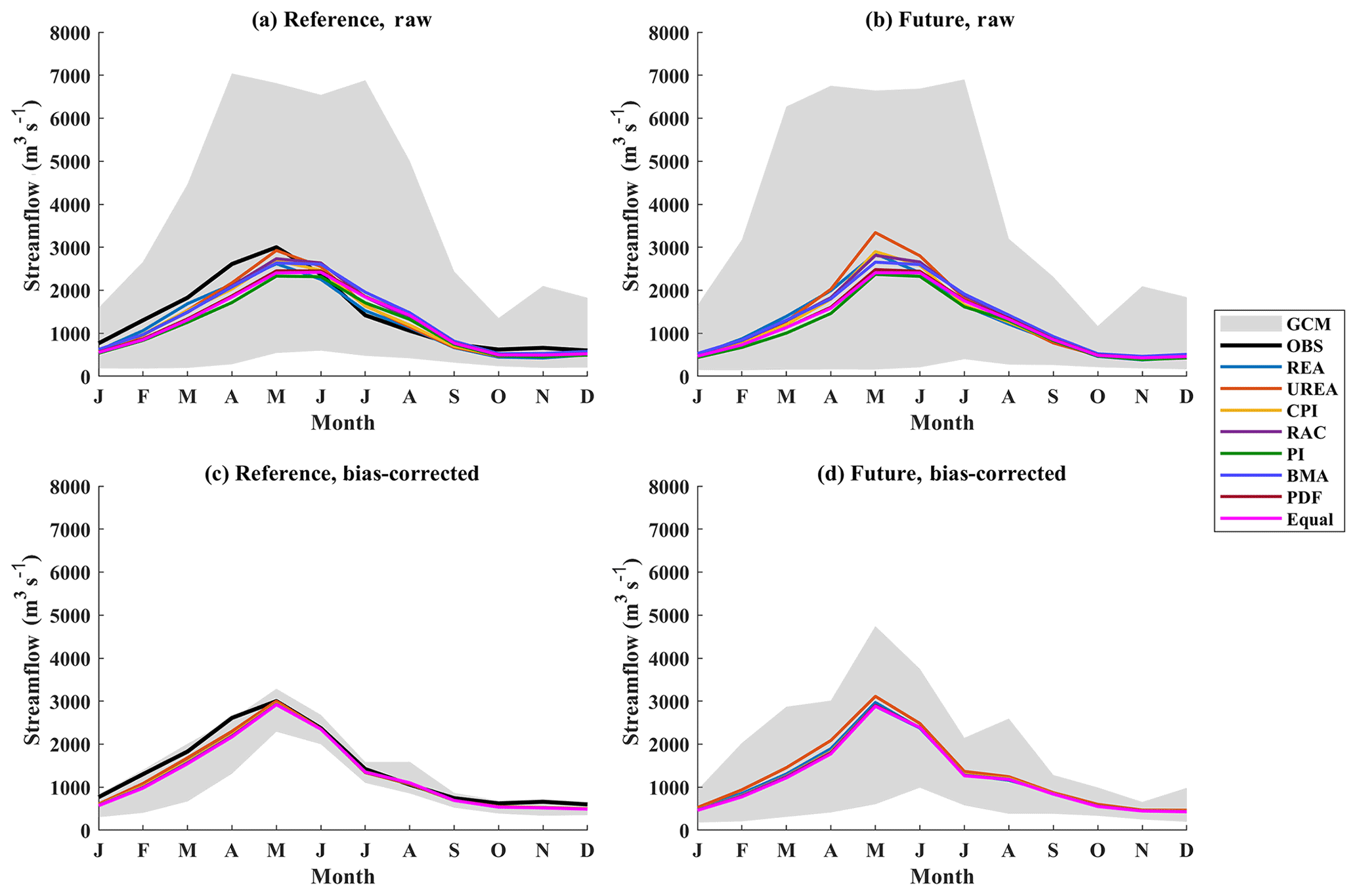
Figure 3 The envelope of monthly mean streamflows simulated by 29 raw and bias-corrected GCM outputs and the multi-model ensemble means of monthly mean streamflows weighted by eight weighting methods based on GCM-simulated streamflows over the Xiangjiang watershed for the reference and future periods (OBS is the hydrograph simulated from meteorological observation).

4.2 Impacts on the hydrological regime

The weights determined by eight weighting methods were first utilized to combine GCM-simulated streamflow series. Figure 3 shows the weighted multi-model mean of monthly mean streamflow for the Xiangjiang watershed. The gray envelope represents the range of monthly mean streamflow simulated using 29 GCM simulations. At the reference period, streamflows simulated by raw GCMs cover a wide range (Fig. 3a). However, the equally weighted multi-model mean streamflow performs better than most of the streamflow series simulated by individual GCMs with respect to reproducing the observed streamflow; even so, the equally weighted ensemble mean still underestimates the streamflow before the peak (January–May) and overestimates it after the peak (June–September).

For the ensemble mean combined by unequal weights, the three weighting methods that generate highly differentiated weights (REA, UREA, and CPI) outperform the equal-weighting method with respect to reproducing the observed monthly mean streamflow. The BMA and RAC methods improve the performance of streamflow simulations before the peak at the cost of performance after the peak, while an opposite pattern is observed when using the PI method. The PDF method generates an ensemble mean of monthly mean streamflows almost identical to that of the equal-weighting method. This is an expected result, as the PDF method assigns almost identical weights to all GCM simulations.

Weights calculated based on the raw temperature and precipitation of GCM outputs were also used to construct the ensemble mean of monthly mean streamflows (Fig. S3a and b). Particularly, for the weights based on raw temperature, the ensemble mean hydrographs combined by the REA, UREA, and CPI methods largely deviate from the observation. Although REA, UREA, and CPI generate highly differentiated weights in this case, their ensemble mean streamflows are significantly inferior to those combined by equal weights (Fig. S3a). In addition, when using raw precipitation to calculate weights, the weighting methods perform worse than or similar to those calculated based on streamflow series (Fig. S3b). This reflects the advantage of streamflow-based weights in terms of reproducing the observed mean hydrograph.

The bias-correction method can reduce the biases of precipitation and temperature in representing the mean monthly streamflow for the reference period, as indicated by the narrowed envelope (Fig. 3c), although a small amount of uncertainty is still observed. The reduction in biases brings about similar weights for all ensemble members in the experiment of using bias-corrected GCM-simulated streamflows. Thus, the multi-model ensemble means of monthly mean streamflow constructed by all unequal-weighting methods are very similar to those constructed by the equal-weighting method, as shown in Fig. 3c.

Figure 4 The same as Fig. 3 but for the Manicouagan-5 watershed.

For the bias-corrected GCM-simulated streamflow in the future period (Fig. 3d), a larger uncertainty related to the choice of climate models is observed, as indicated by the wider envelope of the mean monthly streamflow. This may be because the bias of GCM outputs is nonstationary. All bias-correction methods are based on a common assumption that the bias of climate model outputs is constant over time. However, this assumption may not always be true because of natural climate variability and climate sensitivity to various forcings (Hui et al., 2019; Chen et al., 2015), and most weighting methods still follow the same assumption. In other words, the bias nonstationarity implies that climate models differ in their ability to simulate the climate for the reference and future periods. The weights calculated in the reference period may not be applicable in the future period. The results of this study also prove this, as all of the weighting methods project similar ensemble means of monthly mean streamflows for the future period.

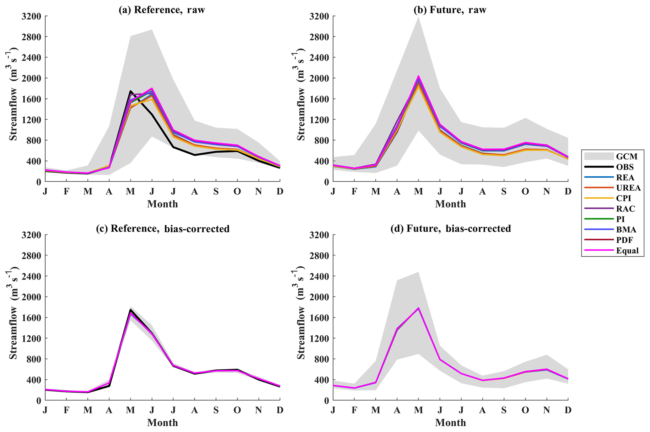
Figure 4 presents the same information as Fig. 3 but for the Manicouagan-5 watershed. Nearly half of the monthly mean streamflow time series simulated by raw GCM outputs have delayed peak (June) compared to the observed one (May) at the reference period, which leads to the delayed peak streamflow of the weighted multi-model mean streamflows for all weighting methods (Fig. 4a). Nonetheless, when raw GCM-simulated streamflow series are used to calculate weights, the multi-model mean streamflows perform better than or similar to those calculated by weights based on raw temperature and precipitation (Fig. S3c). However, for the bias-corrected streamflow series, the uncertainty of monthly streamflows simulated by individual GCMs is largely reduced and the problem of delayed peak streamflow is corrected (Fig. 4c). Similar to the case in the Xiangjiang watershed, all unequally weighted multi-model mean streamflows are identical to those of the equal-weighting method. For the future period, although the uncertainty of single bias-corrected GCM-simulated streamflows increases (Fig. 4d), there are still very few differences among the future multi-model mean streamflows combined by different weighting methods.

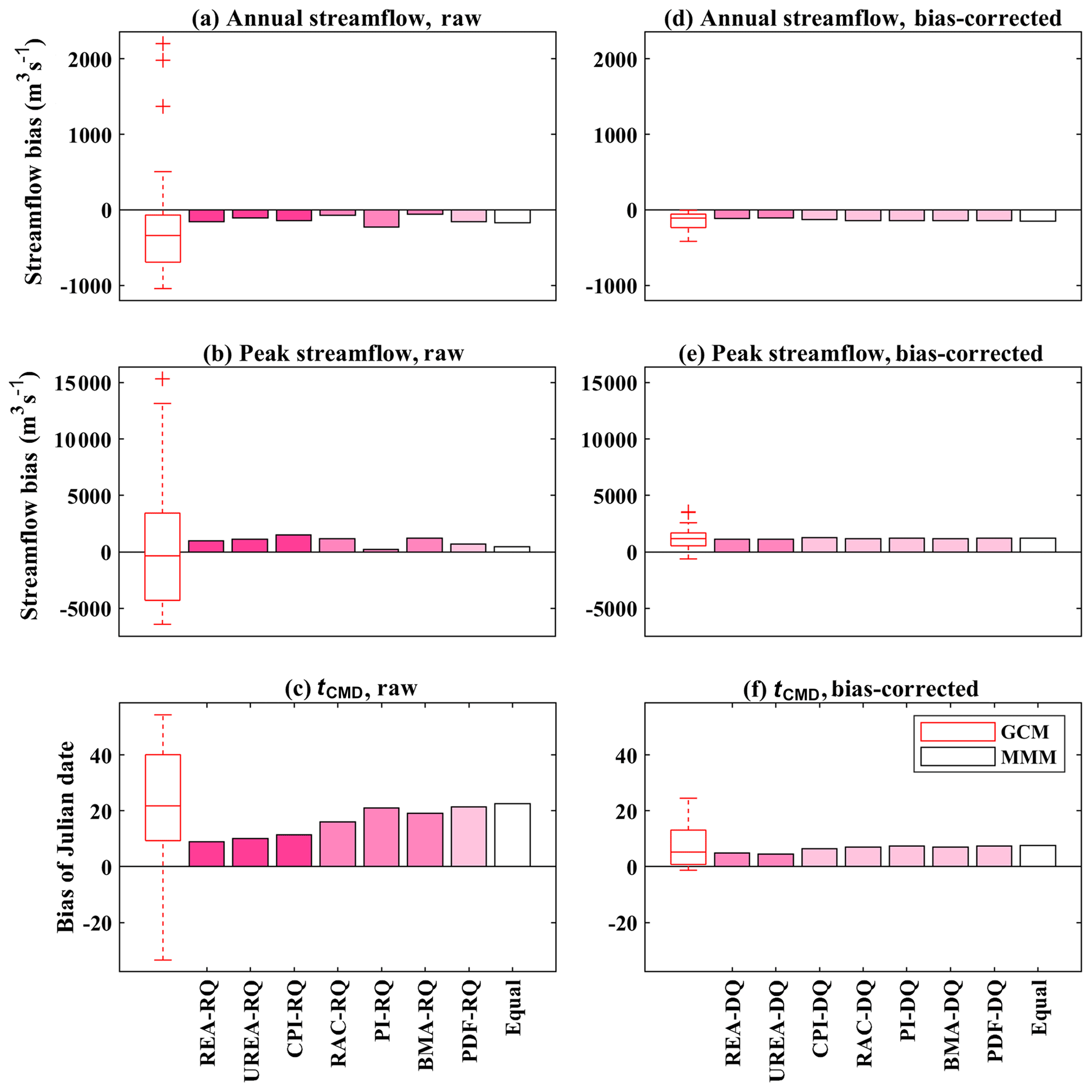
Figure 5 Bias in mean annual streamflow, mean peak streamflow, and mean center of timing of annual flow (t_CMD) simulated using 29 raw or bias-corrected GCM outputs and the multi-model means (MMM) combined by weights based on raw (RQ) and bias-corrected (DQ) GCM-simulated streamflows in the Xiangjiang watershed in the reference period. (The depth of pink in the MMM bars represents the level of inequality of weights, as indicated in Table 3.)

4.3 Bias in multi-model mean

In order to quantify the performances of weighting methods with respect to reproducing the multi-model ensemble mean, biases of the multi-model ensemble mean relative to observation were calculated for the reference period in terms of three hydrological indices (mean annual streamflow, mean peak streamflow, and mean center of timing of annual flow; t_CMD). A smaller bias represents a better performance. Figure 5 presents the biases of weighted multi-model mean indices over the Xiangjiang watershed. For the streamflows simulated using raw GCM outputs, the weighting methods show varied performance in terms of reproducing observed indices (Fig. 5a–c). Except for the PI method, the unequally weighted multi-model means more or less outperform the equal-weighting method in terms of reducing biases in mean annual streamflow and mean t_CMD, while an opposite result is observed in mean peak streamflow. This may be because only the mean value (climatological mean or monthly mean series) was used as the evaluation metric when weights are determined, while peak or extreme values were not considered. Additionally, weights based on the raw temperature and precipitation of GCM outputs were used to calculate multi-model mean indices for comparison (Fig. S4a–c). When raw temperature series are used to determine weights, they often bring about more biases in mean annual streamflow and t_CMD. The weights based on raw precipitation show some superiority in reducing bias in mean peak streamflow. However, in the experiment of using bias-corrected GCM-simulated streamflows to calculate weights (Fig. 5d–f), the biases in multi-model mean indices are much less varied among different weighting methods. This is similar to the previous results of hydrological regimes.

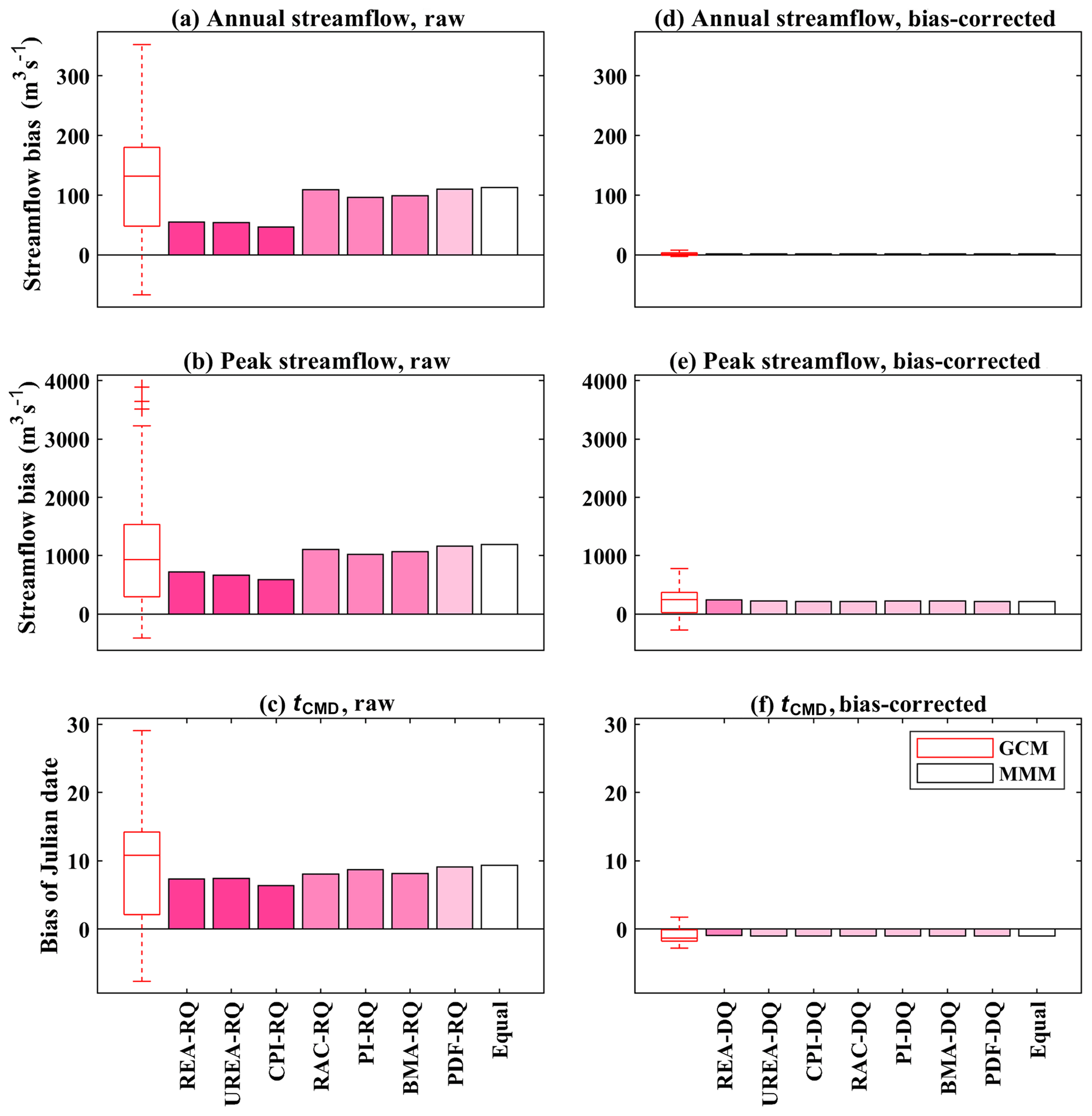
For the case in the Manicouagan-5 watershed (Fig. 6), 25 of the 29 streamflow series simulated by raw GCMs have larger mean annual streamflows and mean peak streamflows than those of the observations, and 26 series generate a delayed t_CMD. This leads to the overestimation of multi-model mean indices for all weighting methods (Fig. 6a–c). Compared to the equal-weighting method, all unequal-weighting methods more or less overcome this overestimation. The three weighting methods that generate highly differentiated weights (REA, UREA, and CPI) notably reduce biases for all three hydrological indices. For most weights calculated based on raw temperature and precipitation of GCM outputs (Fig. S4d–f), a certain improvement in mean indices was also observed (the only exception is raw-precipitation-based PDF weights), but compared to the weights calculated using streamflow series, nearly all streamflow-based weights reduce more biases than those based on temperature and precipitation. However, if bias-corrected GCM-simulated streamflows are used (Fig. 6d–f), again, all weighting methods generate very similar mean indices to the equal-weighting method.

Figure 6 The same as Fig. 5 but for the Manicouagan-5 watershed.

4.4 Impacts on uncertainty

In addition to the multi-model ensemble mean, the impacts of weighting GCM simulations on uncertainty of hydrological responses were also assessed. Figures 7 and S5 present the box plots of changes in four hydrological indices (mean annual streamflow, mean streamflow during the high- and low-flow periods and mean peak streamflow) between the reference and future periods. The box plots of the equal-weighting method are depicted through 29 values simulated by climate simulations, while the box plots of seven unequal-weighting methods are constructed using 1000 values sampled by the Monte Carlo approach based on assigned weights. For example, a simulation with 2 times the weight of another simulation will occur 2 times as often as that in the 1000 samples of Monte Carlo experiments. While the 1000 samples still only consist of 29 values, the occurrence of each value reflects its possibility to be chosen and presents the uncertainty related to the choice of GCMs determined by assigned weights.

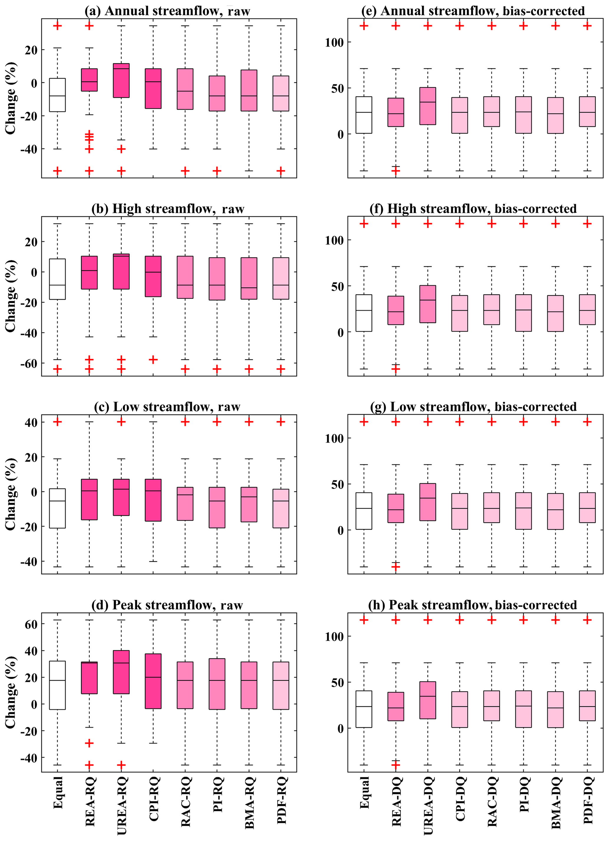
Figure 7 Box plot of changes in four hydrological indices calculated by raw or bias-corrected GCM-simulated streamflows in the Xiangjiang watershed. The changes of hydrological variables were sampled through the Monte Carlo approach based on the weights calculated using raw (R_Q) or bias-corrected (D_Q) GCM-simulated streamflows. (The depth of pink represents the level of inequality of the weights.)

Figure 7 presents the uncertainty of hydrological changes for the Xiangjiang watershed. In the experiment of using raw GCM-simulated streamflows (Fig. 7a–d), depending on the weighting methods, unequal weights show varying effects on the uncertainty. Both the PDF and PI methods suggest similar uncertainties to those of the equal-weighting method for all four hydrological indices. The BMA and RAC methods generate slightly larger uncertainty for the change in mean annual streamflow and slightly smaller uncertainty for the change in low streamflow. The two weighting methods that generate the most differentiated weights (REA and UREA) largely reduce the uncertainty and increase the changes of the upper and lower probabilities for all four hydrological variables. The impacts of weights calculated based on raw GCM temperature and precipitation series were also analyzed (Fig. S6a–d). When weights are calculated based on raw temperature, REA, UREA, and CPI tend to aggressively reduce the uncertainty in mean high streamflow and peak streamflow. Precipitation-based weights show similar influences on uncertainty to the weights based on streamflows. However, for the bias-corrected GCM-simulated streamflows (Fig. 7e–h), the uncertainty of changes in the four hydrological indices is similar among all weighting methods.

The uncertainty of hydrological impacts in terms of four hydrological indices over the Manicouagan-5 watershed is shown in the Supplement (Fig. S5). For weights calculated using raw GCM-simulated streamflows (Fig. S5a–d), only UREA clearly reduces the uncertainty for mean annual streamflow. The REA, UREA, and CPI methods reduce the uncertainty for mean low streamflow and decrease its value of upper probability. There are few differences in the uncertainty of mean high streamflow and peak streamflow among all weighting methods. However, when bias-corrected GCM-simulated streamflows are used (Fig. S5e–h), again, the uncertainty of changes in all four hydrological indices is very similar among most of the weighting methods. Only CPI suggests slight increases in changes of the lower probability.

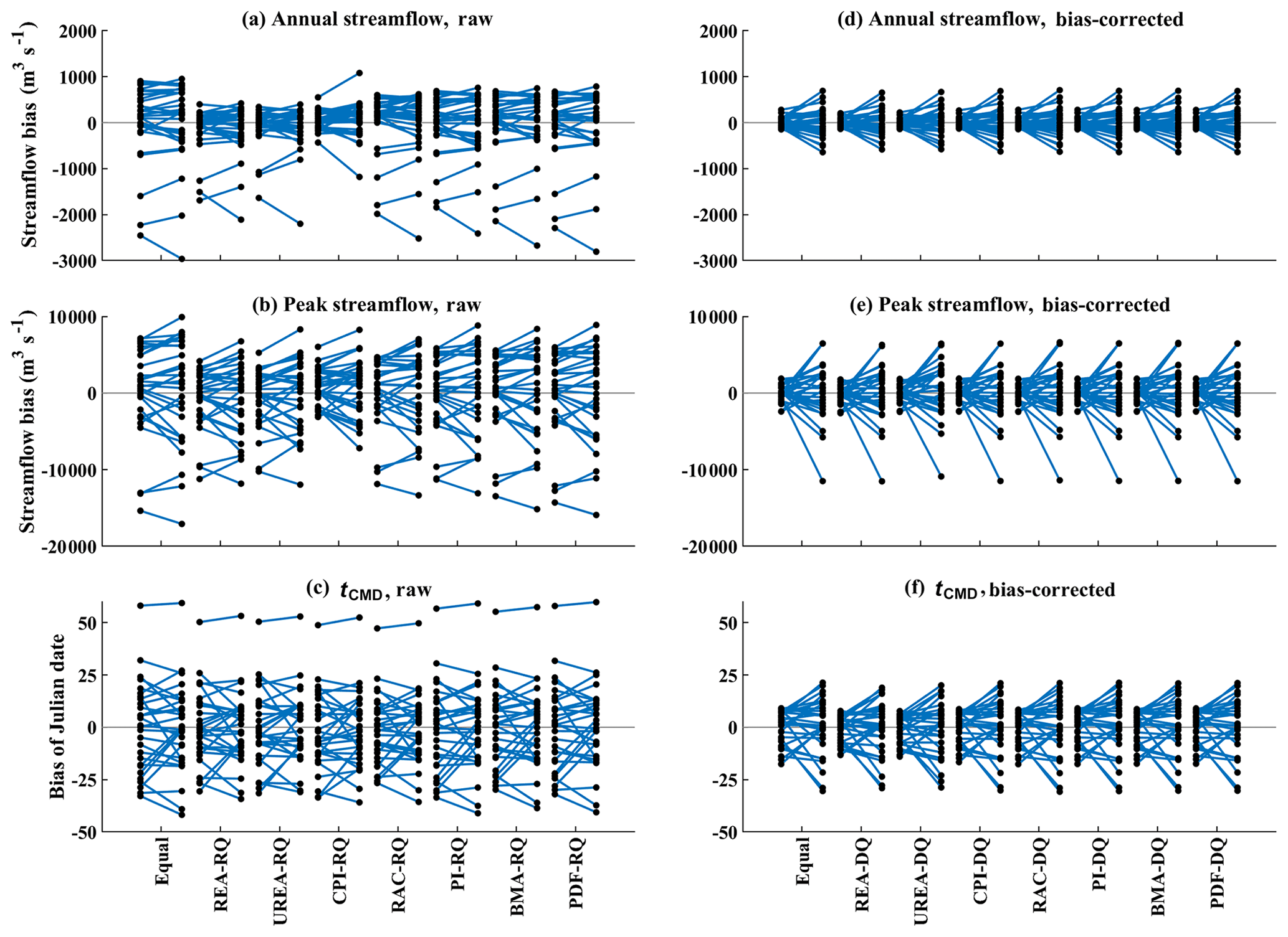
Figure 8 Bias in mean annual streamflow, mean peak streamflow, and mean center of timing of annual flow (t_CMD) of weighted multi-model ensemble mean in the out-of-sample testing over the Xiangjiang watershed; 29 lines of each weighting method represent the results when each of 29 climate models was regarded as the “truth” in turn, and the left and right points on each line represent the biases for the reference and future periods, respectively.

4.5 Out-of-sample testing

In the above assessments except that of the impacts on uncertainty, the weighting methods are mostly evaluated in terms of their performances in simulating observations in the reference period. This kind of assessment has been referred to as “in-sample” testing (Herger et al., 2018). But the performances of weighting methods in the future period (“out-of-sample” testing) may also need to be investigated. However, there are no observations to be compared with in the future period. Thus, an out-of-sample testing was then performed by conducting model-as-truth experiments (Herger et al., 2018; Abramowitz et al., 2019). In model-as-truth experiments, the output of each climate model was regarded as the “truth” in turn, and the outputs of the remaining 28 climate models were used as simulations of this truth model. Then, the weights were recalculated for these remaining models. Since there is a truth in the future period in this case, the performances of weighting methods can be evaluated in terms of reproducing the future truth.

Figure 8 shows the results of out-of-sample testing over the Xiangjiang watershed for biases of weighted multi-model mean hydrological indices, which are the same as those in Fig. 5. The left and right sides of each line respectively represent the biases at the reference and future periods when one climate model is regarded as the truth. Similar to Fig. 5, the bias of weighted mean being closer to zero means that the corresponding weighting method performs better. In general, the results of out-of-sample testing are similar to those where historical observations are used. For the experiment of streamflows simulated by raw GCM outputs, Fig. 8a–c show that unequally weighted means more or less become closer to the truth simulation than those of equal weighting for both reference and future periods. The unequal streamflow-based weights can help to reduce the biases. In particular, the three methods with the most differentiated weights (REA, UREA, and CPI) reduce more biases of annual streamflow when compared with other methods in that the ranges of the biases calculated by these three methods are narrower and closer to zero. In addition, although the biases in the future period tend to be larger than those in the reference period, the unequally weighted means still have a slight improvement in most cases. However, for the experiment of using bias-corrected GCM outputs to simulate streamflows, as shown by the similar patterns among weighting methods (Fig. 8d–f), the unequally weighted multi-model means have similar biases to those of using equal weighting at both reference and future periods. In addition, the results of out-of-sample testing over the Manicouagan-5 watershed are shown in the Supplement (Fig. S7), and generally, they are also similar to the results of using observations (Fig. 6).

5 Discussion

Model weighting is a necessary process in dealing with multi-model ensembles in impact studies. No matter whether bias correction is applied before driving the hydrological model or not, a decision on the weighting methods is always necessary in order to obtain multi-model mean or uncertainty evaluation. Besides the common equal weighting, many studies have proposed unequal-weighting methods in order to obtain a better quantification on climate change, such as a more reliable multi-model ensemble mean or constrained uncertainty (e.g., Giorgi and Mearns, 2002; Sanderson et al., 2017; Xu et al., 2010; Min et al., 2007; Murphy et al., 2004). Most of these studies only use climate variables to determine weights, which may cause two problems for impact studies: uncertain trade-off between multiple variables and a nonlinear relationship between climate and impact variables. Actually, the results of this study reflect these problems. Some examples are the weights based on temperature in the experiment of raw GCM-simulated streamflows in the Xiangjiang watershed (Fig. S3), which lead to obviously biased multi-model mean hydrographs at the reference period. But using the weights calculated based on raw GCM precipitation does not lead to such biases. This may be because the runoff generation in the Xiangjiang watershed is dominated more by rainfall than temperature. In this case, weights calculated using temperature may not reflect a GCM's reliability in terms of hydrological responses. On the contrary, for the snow-dominated Manicouagan-5 watershed (Fig. S3), the snowmelt-driven spring flood is an important characteristic of its hydrological regime, and both temperature and precipitation conditions have large influences on this process. Thus, weights based on temperature and precipitation do not lead to obviously biased multi-model mean hydrographs in this case. Furthermore, over both watersheds, most weights based on raw GCM-simulated streamflows reduce more biases of the mean annual streamflow than those based on raw temperature and precipitation (Figs. 5 and 6). This is as expected because weights based on streamflows directly reflect how GCM simulations conform to the observed streamflow and are not affected by the nonlinear relationship between climate variables and impact variables. Generally, in the experiment of using raw GCMs to simulate streamflows, weights calculated based on streamflows not only circumvent the above two problems but also bring about smaller biases in mean annual streamflow for the multi-model means.

In addition, this study considered the differences in performances of weighting methods when the bias-correction method is applied or not. As shown in Figs. 3 and 4, biases in the simulated mean monthly streamflows are greatly reduced for the reference period after bias correction. This is also observed in other studies (e.g., Chen et al., 2017; Hakala et al., 2018). This change in biases affects the ability of most unequal-weighting methods to discriminate the performances of climate simulations. In this experiment, all of the weighting methods assign similar weights to all simulations (as indicated by the decline of entropy of weights calculated by each weighting method). This is because climate simulations become rather close to each other in the reference period, and all weighting methods except REA in this study only rely on reference performances. As for the REA method, even though it considers future projections in its convergence criterion when calculating weights and its weights are still the most differentiated for the bias-corrected ensemble (as shown in Fig. 2), they have little impact on the final results of the multi-model mean. In addition, the PI method considers independence among simulations, but it only relies on reference values which have been tuned by the bias-correction method. The ability of independence criterion may be affected because of the bias correction. In general, in this experiment, compared to the equal-weighing method, unequal-weighting methods do not bring about much disparateness to the results of hydrological impacts. The out-of-sample testing also manifests the same phenomena. Therefore, in hydrological impact studies, it is likely that using equal weighting is viable and sufficient in most cases when bias correction has been applied. Admittedly, even though most of bias-correction methods can reduce the bias of climate model simulations in terms of a few statistical metrics, no bias-correction methods are perfect for removing all the biases. Besides this, hydrological simulations reflect the overall performance of climate simulations, and small biases in climate simulations (in terms of a few metrics) may results in large biases in hydrological simulations, especially taking nonlinear processes from climate to hydrology worlds into account. Thus, if unequal-weighting methods consider criteria that are different to the bias correction, they may have the potential to induce a better quantification of hydrological impacts. This problem deserves further study.

Despite the choices of variables used to calculate weights, the establishment of any weighting method involves subjective choices of diagnostic metrics, its translation to performance measurement, and normalization to weights (Knutti et al., 2017; Santer et al., 2009). For example, in the RAC method, the correlation coefficient and standard deviation are used as diagnostic metrics, and GCM skills are measured through the translation of a 4th-order formulation. The skill scores are then divided by their sum to be normalized. Any of these steps can ultimately affect the property of a weighting method. For example, the REA, UREA, and CPI methods are inclined to generate more differentiated weights, while other methods assign more similar weights to ensemble members. All of these aspects in weighting methods are often predefined without detailed examination or are based on expert experience and, thus, can actually introduce several layers of subjective uncertainty. An improper weighting method may even cause a risk of reducing projection accuracy (Weigel et al., 2010), and extremely aggressive weighting may conceal the uncertainty rather than reduce it (Chen et al., 2017). Thus, notwithstanding the equal weighting not being a perfect solution, model weighting methods should be used with caution, and the results of equal weighting should be presented along with those of the unequal-weighting method.

Moreover, some risks may exist in the usage of weighting methods in impact studies. Firstly, weights are generally assigned to climate simulations in a static way (i.e., weights in the future period are the same as those in the reference period). This usage shares the same assumption with bias-correction methods that the performances of GCM simulations are stable and stationary. However, some studies have shown that model skills are nonstationary in a changing climate (Weigel et al., 2010; Miao et al., 2016), and models with better performance in the reference period do not necessarily provide more realistic signals of climate change (Reifen and Toumi, 2009; Knutti et al., 2010). The way to deal with the dynamic reliability of climate models in weighting methods deserves further study. Secondly, many researchers and end users in hydrological impacts only consider one diagnostic metric to determine weights, such as the climatological mean (e.g., Wilby and Harris, 2006; Chen et al., 2017). It is not clear whether reducing the bias of one specific metric can transfer to other metrics. The weights calculated using the raw GCM-simulated streamflows in the Xiangjiang watershed are one negative example, where the bias in mean annual streamflow is reduced while the bias in the mean peak streamflow is enlarged. Some studies have also shown similar problems (Jun et al., 2012; Santer et al., 2009). For example, Jun et al. (2012) demonstrated that there is little relationship between a GCM's ability to reproduce mean temperature state and trend of temperature. Actually, a set of metrics can be introduced to determine weights (e.g., Sanderson et al., 2017). Some studies suggested using calibrated multiple metrics because it can improve the rationality of weighted multi-model mean (Knutti et al., 2017; Lorenz et al., 2018), while some argued that multiple metrics form another level of uncertainty within weighting methods (Christensen et al., 2010). Thus, the best way to choose proper metrics and synthesize performances in multiple metrics still remains in doubt and deserves further research.

There is a limitation in the hydrological modeling in this study. Only large watersheds as well as a lumped hydrological model were considered. When a lumped model is used, the nonlinear relationship between the climate variables and the impact variable (streamflow) may not be sufficiently revealed. Spatial differences between different climate simulations only affect the basin-averaged inputs to the hydrological model but do not directly affect the process of runoff generation and streamflow routing (Lebel et al., 1987). Temporal variations in climate simulations may be partially reduced by the lumped hydrological model as well. With the help of other more sophisticated hydrological models (such as distributed models), the differences between climate-based weights and streamflow-based weights may become more obvious. For the experiment of raw GCM-simulated streamflows, the weights based on streamflow perform better than those based on climate variables. This may be related to large differences among climate simulations. But in the experiment of streamflows simulated using bias-corrected GCM outputs, the fact that not much discrepancy is seen in the performances between unequal and equal weighting may be partly because only a simple hydrological model is used. In other words, the remaining differences among corrected climate simulations may not be presented well in streamflow simulations when a lumped hydrological model is used in such large watersheds.

In addition, the other limitation is that this study only considered two watersheds in humid regions. If weights are determined on climate variables for watersheds in different climate regions, they may manifest different performances in the hydrological impacts. For example, for arid watersheds, whose hydrological regime is more characterized by the intense flow and evaporation, a proper combination for the weights based on temperature and precipitation may be necessary in order to obtain a better quantification. For urban watersheds, storm water contributes to their runoff and weights based on precipitation intensity may be more advantageous. Nevertheless, based on the results of this study, using impact variables to determine weights may help to circumvent the problem of trade-off and choice of climate variables. However, specific advantages of weights based on impact variables and influences of bias correction on the performances of weighting methods in other types of watersheds still deserve site-specific research.

6 Conclusion

In order to weight climate models based on the impact variable and to quantify their influences on the impact assessment, this study assigns weights to an ensemble of 29 CMIP5 GCMs over two watersheds through a group of weighting methods based on GCM-simulated streamflow time series. Streamflow series are simulated by separately inputting the raw and bias-corrected GCM simulations to a hydrological model. Using streamflows to determine weights is straightforward and can avoid the difficulty of combining weights based on multiple climate variables. The influences of these unequal weights on the assessment of hydrological impacts were then investigated and compared to the common strategy of model democracy.

This study concludes that for the streamflows simulated using raw GCM outputs without bias correction, unequal weights have some advantages over the equal-weighting method in simulating observed mean hydrographs and reducing the biases of multi-model mean in mean annual streamflow. In particular, the weights calculated based on streamflows can reduce more biases of multi-model mean annual streamflow and better reproduce observed hydrographs compared with the weights calculated based on climate variables. However, when using bias-corrected GCM outputs to simulate streamflow, GCM simulations are brought close to the observations by the bias-correction method. Consequently, the weights assigned to climate simulations become similar to each other, resulting in similar multi-model means and uncertainty of hydrological impacts for all unequal-weighting methods. Therefore, the equal-weighting method is still a conservative and viable option for combining the bias-corrected multi-model ensembles, or, if an unequal-weighting method is applied, it is better to present it to end users with a detailed explanation of the weighting procedure as well as the results of using the equal-weighting method.