State updating and calibration period selection to improve dynamic monthly streamflow forecasts for an environmental flow management application

Monthly to seasonal streamflow forecasts provide useful information for a range of water resource management and planning applications. This work focuses on improving such forecasts by considering the following two aspects: (1) state updating to force the models to match observations from the start of the forecast period, and (2) selection of a shorter calibration period that is more representative of the forecast period, compared to a longer calibration period traditionally used. The analysis is undertaken in the context of using streamflow forecasts for environmental flow water management of an open channel drainage network in southern Australia. Forecasts of monthly streamflow are obtained using a conceptual rainfall–runoff model combined with a post-processor error model for uncertainty analysis. This model set-up is applied to two catchments, one with stronger evidence of non-stationarity than the other. A range of metrics are used to assess different aspects of predictive performance, including reliability, sharpness, bias and accuracy. The results indicate that, for most scenarios and metrics, state updating improves predictive performance for both observed rainfall and forecast rainfall sources. Using the shorter calibration period also improves predictive performance, particularly for the catchment with stronger evidence of non-stationarity. The results highlight that a traditional approach of using a long calibration period can degrade predictive performance when there is evidence of non-stationarity. The techniques presented can form the basis for operational monthly streamflow forecasting systems and provide support for environmental decision-making.

1 Introduction

Predictions of streamflow a month or a season ahead are essential information required by water resource managers for subsequent planning (Wang et al., 2011). This is particularly true in unregulated catchments with no capacity for storage and a highly variable flow regime that can be difficult to predict from historical data. A number of approaches have been developed to provide streamflow predictions with lead times from a month to a season ahead. These include “dynamic” hydrological modelling approaches (Demargne et al., 2014; Wood and Schaake, 2008), statistical approaches (Bennett et al., 2014; Robertson and Wang, 2013), or a combination of the two (Robertson et al., 2013).

In this work, a dynamic hydrological modelling based approach is adopted to provide streamflow forecasts for an environmental management application. The dynamic approach can often better capture catchment dynamics than statistical models based on simple climatic indices (Robertson et al., 2013). In forecast mode, a hydrological model calibrated using historical data is run forward in time, with input data provided by forecast climate forcings. The following three major factors control forecasting performance (Luo et al., 2012): (1) the ability of the hydrological model to predict streamflow with actual forcings; (2) the accuracy of the assumed initial conditions (e.g. soil moisture stores); and (3) the accuracy of the forecasts of the climate inputs. The focus of this paper is on the first two factors, in the context of a user need for monthly streamflow forecasts to support environmental management and decision-making.

Conceptual rainfall–runoff (CRR) models are widely used to simulate streamflow, due to their simplicity and accuracy (Li et al., 2015a; Tuteja et al., 2011). The parameters of these models have a limited relationship with measurable catchment attributes (e.g. soil horizon depth; Fenicia et al., 2014), and typically require calibration to observed streamflow data (noting that physical models also require some calibration; Mount et al., 2016; Pappenberger and Beven, 2006). The use of long calibration periods assumes time-invariant catchment characteristics and processes, and that the parameter values derived from the calibration period are representative of the prediction period (Vaze et al., 2010). It is generally considered that longer calibration periods produce more robust parameter estimates, as a longer period exposes the model to a more diverse range of catchment conditions and flow events (Wu et al., 2013); however, this is not always the case (for example, Brigode et al., 2013).

The assumption that parameters are constant in time can result in decreased model performance if the conditions encountered in the forecast period are different from those in the calibration period (Bowden et al., 2012; Coron et al., 2012). In this work, the term “non-stationary” is used to refer to situations where physical changes are expected to have occurred in a catchment, and where there is evidence to reject the hypothesis of stationarity. In practice, catchments may have different “degrees” of non-stationarity, depending on the evidence available to reject the hypothesis of stationarity, the degree of change in a catchment, and the timescales over which the changes take place. Examples of catchment non-stationarity that can be expected to change the rainfall–runoff relationship include changes in land use or land cover (e.g. deforestation, urbanisation), land drainage, interception (e.g. dams, diversions), groundwater abstractions or responses to changes in climate (Milly et al., 2015). This definition of catchment non-stationarity can be contrasted to a broader definition of “hydrological model non-stationarity”, which refers to temporal changes in hydrological model parameters for any reason (e.g. systematic data errors, poor calibration procedures, model structural deficiencies); see, for example, Westra et al. (2014).

The degradation in model predictive performance due to catchment non-stationarity can impact on the decisions informed by these forecasts. To address this concern, a number of studies have calibrated model parameters to subsets of the available data, by attempting to find periods in the historical record that are analogous to conditions expected in the prediction time period, and by tailoring the time period selection to compensate for deficiencies in the model structure or input data (Brigode et al., 2013; de Vos et al., 2010; Luo et al., 2012; Vaze et al., 2010; Wu et al., 2013; Zhang et al., 2011). Often there is a trade-off between the benefits of a longer calibration period, which exposes the model to a more diverse range of conditions and tends to improve parameter identifiability, versus the benefits of a shorter calibration period, which exposes the model to the most recent – and hence often the most relevant – dynamics in the catchment. Demonstrating and understanding the impact of this trade-off on model predictive performance is a key research gap pursued in this study.

Predictive uncertainty quantification is another major aspect of practical streamflow prediction. Many approaches are available to quantify predictive uncertainty, from approaches that identify a range of model parameters that represent the behaviour of the catchment using approaches such as generalised likelihood uncertainty estimation (GLUE; Beven and Binley, 1992), to post-processor approaches (e.g. Krzysztofowicz and Maranzano, 2004) and disaggregation approaches that attempt to characterise each individual source of error explicitly (e.g. Kavetski et al., 2003; Vrugt et al., 2005). In this work, predictive uncertainty is estimated using an aggregated post-processor residual error model. The residual error model represents the differences between the hydrological model predictions and observed data, without trying to identify the contributing sources (Evin et al., 2014). The post-processor approach is chosen because it can lead to more robust estimates of predictive uncertainty compared to joint calibration of all parameters (i.e. estimating CRR model and error model parameters concurrently; Evin et al., 2014).

Much of the skill in seasonal streamflow forecasts over periods following rainy seasons is commonly attributed to accurately representing initial catchment conditions (Koster et al., 2010; Pagano et al., 2004; Wang et al., 2009). In contrast, forecast skill over periods following dry seasons is generally attributed to both initial catchment conditions and meteorological inputs (Maurer and Lettenmaier, 2003; Wood and Lettenmaier, 2008). The impact of the initial catchment conditions is particularly pronounced when forecasting over short lead times, typically up to 1 month (Li et al., 2009; Wang et al., 2011), although this time frame is generally catchment-dependent.

Figure 1 Map of the case study region, in southern Australia.

In CRR models, catchment conditions are represented by (usually multiple) model storages, referred to as “state variables”. The values of these storages at the start of a forecast period are typically determined using a warm-up period, which allows the internal model states to reach reasonable values. Given the expected influence of the initial conditions on the simulated streamflow, observed data can be assimilated into the model to update the state of the model storages. The most commonly used approaches in hydrological data assimilation include direct updating of storages (for example, Demirel et al., 2013), Kalman filtering, particle filtering, and variational data assimilation (see Liu and Gupta, 2007). Berthet (2010) considered a number of tests for different updating approaches for the GRP model, a CRR model commonly used in short-term streamflow forecasting applications in France.

Updating the states of conceptual rainfall–runoff models is not straightforward, as any environmental model is at best an approximate representation of the real catchment (Berthet et al., 2009). A number of observed data sources can be used to update model storages, including observed streamflow and in situ or remotely sensed soil moisture. From these options, Li et al. (2015b) suggest that gauged discharge data assimilation is a more effective way to improve short-term forecasts and is still preferred for operational streamflow forecasting purposes.

Studies on observed data assimilation and CRR model state updating have focused primarily on flood forecasting with short lead times. The benefits at longer lead times (e.g. monthly to seasonal) to forecast water availability have received less attention in the published literature.

1.1 Study aims

This work focuses on determining the degree to which state updating and the selection of calibration period length can enhance monthly streamflow predictions in the context of an environmental flow management application. More specifically, the aims of this study are to

1. evaluate the ability of state updating in a daily CRR model to improve predictive performance when forecasting streamflow volume for the upcoming month; and

2. assess the degree to which using a shorter calibration period that is more representative of the forecast period can improve predictive performance, in particular when there is evidence of catchment non-stationarity.

The paper is organised as follows. Section 2 outlines the user need for monthly forecasts to manage a drainage network for environmental and social outcomes in southern Australia, and describes the case study catchments and data available. Section 3 describes the model set-up and forecasting framework, as well as the methodology designed to achieve the aims above. Sections 4 and 5 present and discuss the case study results, and Sect. 6 summarises the key conclusions.

2 Environmental flow management case study

2.1 Catchment location and characteristics

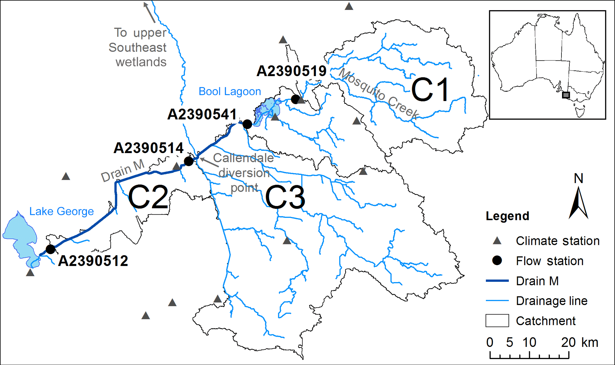
The location considered in this study is a component of an extensive drainage network (exceeding 2500 km of open channels) in southern Australia (Fig. 1). Historically, runoff flowed in a northerly direction, along the watercourses adjacent to ranges, parallel to the coastline. Over the past 150 years, these flow paths have been diverted through a series of cross-country drains, constructed to provide flood relief and improve the agricultural productivity of the region by draining water in a south-westerly direction, creating outlets to the ocean. The largest of these cross-country drains is Drain M (Fig. 1), which conveys water from Bool Lagoon to Lake George. Monthly runoff volumes from Drain M are highly variable, ranging from close to zero to more than is required to support Lake George, with the historical volumes varying over 3–4 orders of magnitude for a given month (Fig. 2). This variability makes it difficult to maximise the use of water, as the seasonal pattern described by the historical record alone provides little guidance.

The streamflow in the case study region is seasonal to ephemeral, with very low flow over the summer and autumn months (Fig. 2). Runoff coefficients are low, with annual runoff in the range of 0.01–0.1 of annual rainfall (Gibbs et al., 2012). The predominant land use in the region is dry land pasture with some flood irrigation as well as plantation forestry; there is no major urbanisation in the catchments. The topography of the region is very flat, with mainstream slopes of the order of 0.005. The hydrogeology of the catchment includes shallow aquifers with major karstification of limestone, which may be suggestive of non-conservative catchments with appreciable groundwater exchanges across their boundaries.

Mosquito Creek flows into Bool Lagoon (catchment C1 in Fig. 1, area 1002 km²). Drain M commences at the outlet of Bool Lagoon, and a large catchment flows into Drain M between Bool Lagoon and a diversion point at Callendale (catchment C3 with an area of 2200 km²). Finally, the Drain M local catchment contributes flow downstream of the Callendale diversion point, flowing into Lake George (catchment C2, area 383 km²).

Figure 2 Variability in monthly runoff in Drain M at the location at flow station A2390512.

In the region where the case study catchments are located, plantation forestry expanded substantially in the late 1990s. Changes in the relationship between rainfall and runoff also occurred during this period, evidenced by the reduced slope in the plot of cumulative runoff against cumulative rainfall (double-mass analysis) in Fig. 3 (Searcy et al., 1960; Yihdego and Webb, 2013). The runoff ratio in catchment C1 is approximately 0.045 before year 2000, but reduces by 70 % to 0.013 after 2000. The runoff ratio in catchment C2 is around 0.088 before year 2000, but reduces by 30 % to 0.061 after 2000. This comparison provides stronger evidence of non-stationarity in catchment C1 than in catchment C2. Other studies have also investigated the link between changes in the hydrology and changes in land use in the region (Avey and Harvey, 2014; Brookes et al., 2017). These changes have implications for the choice of calibration data period, as data from the 1970s may not be representative of hydrological conditions in the 2000s.

It is evident from Fig. 3 that catchment C3, despite having the largest catchment area (2200 km²) of the three catchments, generates very little runoff. This behaviour is due to a number of factors, including the very flat terrain and depression storage, substantial vegetation cover (both plantation and natural) and irrigation extractions from the shallow underlying aquifer. Given its limited streamflow volume, catchment C3 is excluded from further analysis in this study. From a practical perspective, it is assumed that in the years where there is substantial yield from this catchment there will already be surplus flow from the upstream catchments.

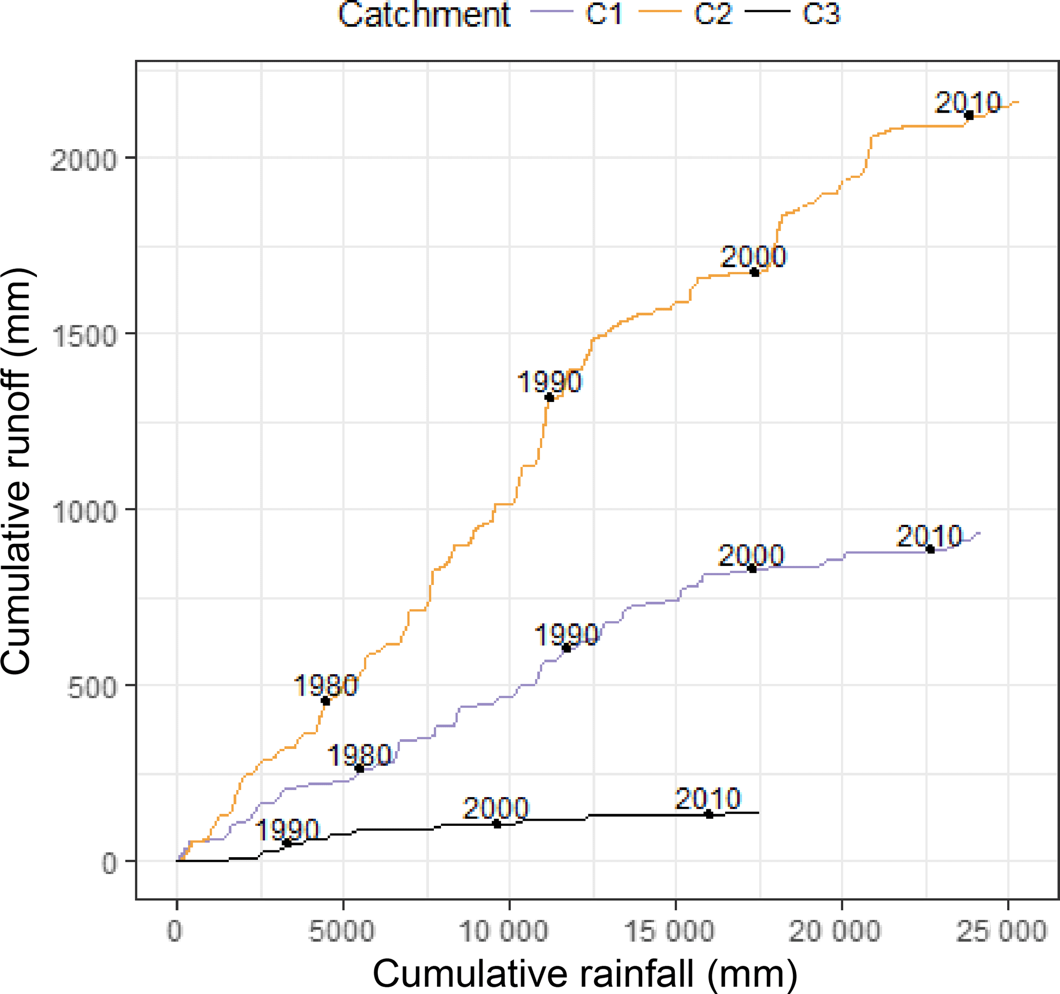
Figure 3 Double mass plot of the rainfall–runoff data in the three main catchments contributing to Drain M. It can be seen that (1) the volume of runoff for the same volume of rainfall has reduced in the latter decade, and (2) very little runoff is generated from catchment C3.

2.2 Management issues

Drain M serves multiple competing demands on the water resources available in this catchment system. These demands influence the decision to use the regulators along the system.

• a.

  Bool Lagoon has water requirements that influence releases from the lagoon into Drain M.

• b.

  Lake George has water requirements to maintain the estuarine ecology of the lake, and to support its significance as a biological resource and as a resource for recreational fishing.

• c.

  The ocean outlet requires some flow to prevent sediment from entering Lake George and to maintain connectivity to the sea (which allows fish movement and aids fish recruitment). However, high flows may impact on sea grasses, due to their low salinity and high nutrient load.

• d.

  The wetlands of the upper south-east to the north typically benefit from as much water as possible from the Drain M system.

Decisions to undertake diversions from Drain M must be made throughout the year (mainly in the high-flow season from late winter and throughout spring). It is expected that forecasts of future flows at key locations will assist in maximising the environmental and social outcomes achieved from the available water. Forecasts of monthly volume with a lead time of 1 month ahead are considered most appropriate for this application, because (1) the main quantities of interest in this application are volume and the overall water balance, rather than the size or timing of daily peak flows, and (2) a 1-month lead time provides sufficient time to undertake any changes in diversions to satisfy the competing demands on the system.

2.3 Climate data

The mean annual rainfall for the region varies from 600 mm in the north to 675 mm in the south. The mean annual FAO56 potential evapotranspiration (PET; Allen et al., 1998) is approximately 1000 mm. The highest rainfalls are experienced in the winter months, with rainfall exceeding evapotranspiration in May–September. The SILO Patched Point Dataset (Jeffrey et al., 2001) was used for the observed rainfall and the FAO56 evapotranspiration data were adopted, with the climate stations used shown in Fig. 1. Time series of rainfall and evapotranspiration in each catchment were obtained using a Thiessen polygon approach. This weighting approach is considered appropriate for the region, due to the flat terrain being unlikely to lead to significant topographic effects on the spatial distribution of rainfall.

Rainfall forecasts from the Australian Bureau of Meteorology's seasonal forecast system, POAMA-2 (Hudson et al., 2011), were used. POAMA-2 is a dynamical climate forecasting system designed to produce multi-week to seasonal forecasts of climate for Australia based on a coupled ocean–atmosphere model and ocean–atmosphere–land observation assimilation systems. In this paper, we use a 30-member ensemble of monthly/multi-week forecasts from version 2.4 of POAMA-2. POAMA-2 predictions have a coarse spatial resolution (∼ 250 km), which does not capture the spatial variability in catchment-scale rainfall. For the purposes of this application, the POAMA-2 rainfall hindcasts (i.e. forecasts developed by applying the modelling system to the historical period) at the relevant pixel were downscaled to each climate station in the study region (Fig. 1) using the statistical downscaling method detailed in Shao and Li (2013). Further details of the downscaling approach are provided in Humphrey et al. (2016).

2.4 Streamflow data

Daily streamflow data are available from the South Australian Department of Environment, Water and Natural Resources Surface Water Archive (https://www.waterconnect.sa.gov.au/Systems/swd), with the flow stations used shown in Fig. 1. Three of the flow stations have data available from the early 1970s, with the exception being the station at the outlet of Bool Lagoon (site A2390541), where data were available from 1985. Travel times along Drain M between flow stations are typically less than 1 day. To determine the flow generated within catchment C2, the daily flows recorded at upstream flow station A2390514 were subtracted from downstream flow station A2390512.

The identification of high-quality data is important because biases and systematic changes in the measurement of hydrological data can significantly affect model calibration and lead to non-stationarity in the estimated model parameters (Westra et al., 2014). Analysis of the data and monitoring stations suggested that streamflow data uncertainty is expected to be low, given the regular cross sections of the weirs used for monitoring stage and upstream drains, and the high number of gaugings (between 78 and 166 flow gaugings at each flow station) available to develop stage–discharge relationships.

3 Methodology

3.1 CRR model

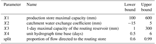
The GR4J model (Perrin et al., 2003) is a parsimonious daily CRR model, selected for this study because it explicitly accounts for non-conservative (or “leaky”) catchments (relevant for the study area; see Sect. 2.1) and has demonstrated good performance for Australian conditions (Coron et al., 2012; Guo et al., 2017; Westra et al., 2014). The standard form of the GR4J model has four calibration parameters: the maximum capacity of a production (soil) store, X1, a catchment water exchange coefficient, X2, the maximum capacity of a routing store, X3, and a time base for a unit hydrograph, X4. Further details of the model structure and parameters can be found in Perrin et al. (2003).

Note that the catchments considered have a relatively slow streamflow response. Consequently, the pre-specified split to the routing store of 0.9 in the original specification of the GR4J model may be too low for these catchments. To mitigate this potential deficiency, we have modified the GR4J model so that the split between the routing store and the direct runoff is included as an explicit calibration parameter termed split.

Table 1 Bounds adopted for the uniform prior distribution on the GR4J parameters.

3.2 Parameter estimation

The GR4J parameters are inferred using Bayes' equation. The posterior probability density of the parameters given daily observed streamflow data $\stackrel{\mathrm{̃}}{q}$ and climate data X, $p\left(\mathit{\theta }\mathrm{|}\stackrel{\mathrm{̃}}{q}\mathbf{X}\right)$, is given by

$$\begin{array}{}\text{(1)}& p(\mathit{\theta }\mathrm{|}\stackrel{\mathrm{̃}}{q},\mathbf{X})\propto p(\stackrel{\mathrm{̃}}{q},\mathrm{|}\mathit{\theta }\mathit{X})p\left(\mathit{\theta }\right),\end{array}$$

where p(θ) is the prior distribution and $p\left(\stackrel{\mathrm{̃}}{q}\mathrm{|}\mathit{\theta },\mathbf{X}\right)$ is the likelihood function.

A standard least squares likelihood function is adopted (see, for example, Thyer et al., 2009), which is derived from a residual error model that assumes independent, homoscedastic residuals. This likelihood function is adopted for the calibration of the daily hydrological model because it provides a better fit to the high daily flows (Wright et al., 2015), which make an important contribution to monthly volumes of interest in our study. Uniform prior distributions are used for all parameters, with bounds given in Table 1.

The posterior distribution in Eq. (1) is sampled using the DiffeRential Evolution Adaptive Metropolis (DREAM) algorithm (Vrugt et al., 2009). The sampled parameter sets are then used to approximate the posterior parameter distribution for a given calibration period. Computations were carried out using the Hydromad R package implementation of the DREAM algorithm and the GR4J model (Andrews et al., 2011). A total of 25 000 iterations of the DREAM algorithm were carried out, including a “burn-in” period of 6250 iterations to allow the Markov chain to stabilise. The number of parallel chains was set equal to the number of parameters (Vrugt et al., 2009), which, for the modified GR4J model used in this work (Sect. 3.1), led to five parallel chains being used.

The posterior distributions obtained for different calibration time periods are investigated for evidence of trends and changes over time. For the purposes of developing streamflow predictions using the post-processing approach (Sect. 3.5), only the single parameter set resulting in the maximum posterior probability is used.

3.3 Calibration approach

A rolling calibration approach is used to account for the impact of non-stationarity on the inferred CRR model parameters. This rolling calibration approach is similar to the approach used by Luo et al. (2012) and Wagener et al. (2003). It consists of choosing a calibration length and then moving it forward year by year, while recalibrating the model parameters to each such calibration “window”. The calibrated parameter values are used to simulate the following 1 year of data, before recalibrating the model and repeating the process. This methodology allows the identification of changes in parameter distributions over time, without the need to identify specific periods when changes in the rainfall–runoff response may have occurred.

Calibration period lengths of CPL = 10 and CPL = 20 years are considered, to assess the trade-off between using a longer calibration period to expose the model to more diverse catchment conditions and improve parameter identifiability, versus using a shorter calibration period length to expose the model to more recent hydrological dynamics.

As an example, consider a 10-year calibration period from 1 May 1995 to 30 April 2005, after a 1-year warm-up period. Predictions are computed for the following 1-year “prediction period”, i.e. 1 May 2005 to 30 April 2006. The process is then repeated each year, i.e. the next calibration period is 1 May 1996 to 30 April 2006, and the calibrated model is used to predict the period 1 May 2006 to 30 April 2007. The starting month of May corresponds to the start of the flow season (Fig. 2).

3.4 State updating in GR4J

The approach used for the state updating of GR4J is similar to the approach of Crochemore et al. (2016) and Demirel et al. (2013). State updating is set to take place at the start of each month within the 1-year prediction period, using the observed streamflow at the start of each month. GR4J has two stores, namely the production store and the routing store. Following the procedure of Demirel et al. (2013), the routing store level is updated such that the GR4J simulation of streamflow matches the observed flow. This procedure is undertaken after accounting for the modelled direct flow from the production store (Demirel et al., 2013).

More specifically, the following procedure is used. In GR4J, the total simulated streamflow on a given day $q_t^{\mathit{\theta }}$ is defined by the sum of the direct flow from the production store (after applying a unit hydrograph), $q_{t,d}^{\mathit{\theta }}$, and the flow from the routing store, $q_{t,r}^{\mathit{\theta }}$,

$$\begin{array}{}\text{(2)}& q_t^{\mathit{\theta }}=q_{t,d}^{\mathit{\theta }}+q_{t,r}^{\mathit{\theta }}.\end{array}$$

Let $q_{t,r}^{\mathrm{SU}}$ denote the flow from the routing store that yields $q_t^{\mathit{\theta }}$ equal to the observed flow $\stackrel{\mathrm{̃}}{q_t}$. This quantity is calculated as

$$\begin{array}{}\text{(3)}& q_{t,r}^{\mathrm{SU}}=\max (\stackrel{\mathrm{̃}}{q_t}-q_{t,d}^{\mathit{\theta }},\mathrm{0}).\end{array}$$

The routing store level, R, can then be obtained by setting $q_{t,r}^{\mathit{\theta }}=q_{t,r}^{\mathrm{SU}}$, and solving (using the bisection method) the equation used by the GR4J model to calculate the outflow from this storage:

$$\begin{array}{}\text{(4)}& q_{t,r}^{\mathit{\theta }}=R\left(\mathrm{1}-{\left(\mathrm{1}+{\left({\displaystyle \frac{R}{X\mathrm{3}}}\right)}^{\mathrm{4}}\right)}^{-\mathrm{1}/\mathrm{4}}\right).\end{array}$$

Equations (2)–(4) can be used to update R given the observed streamflow $\stackrel{\mathrm{̃}}{q_t}$.

3.5 Estimation of predictive uncertainty

The monthly streamflow forecasts are obtained by aggregating the daily GR4J simulations. In order to quantify predictive uncertainty using a residual error model, the monthly aggregated GR4J simulations, Q^θ, are compared to observed monthly streamflow volumes, $\stackrel{\mathrm{̃}}{Q}$. The quantification of error is based on residual errors, defined by the differences between observed and simulated monthly streamflow. Separate error models are estimated for the GR4J predictions for each catchment and for each type of forcing data (observed or forecast rainfall), as follows.

When observed rainfall is used as input to GR4J, the daily streamflow time series simulated using GR4J are aggregated to produce monthly time series of hydrological model predictions, Q^θ.

When forecast rainfall is used as input to GR4J, an ensemble of daily streamflow forecasts is produced (with a single GR4J streamflow time series per rainfall forecast time series). Each such “individual” daily GR4J time series is then aggregated to a monthly time step. The time series Q^θ is constructed from the time series of medians of the individual monthly streamflow time series. Although the use of aggregation approaches for single-valued streamflow forecast from ensemble predictions has been seen in operational applications (see, for example, Lerat et al., 2015), we note that this approach may result in some information loss.

The heteroscedasticity (i.e. larger residuals for larger flows) and skewness of forecast errors is accounted for using the Box–Cox transformation, by defining normalised residuals as

$$\begin{array}{}\text{(5)}& {\mathit{\eta }}_t=Z\left({\stackrel{\mathrm{̃}}{Q}}_t\right)-Z\left(Q_t^{\mathit{\theta }}\right)\end{array}$$

where

$$\begin{array}{}\text{(6)}& Z(Q;\mathit{\lambda },A)=\left\{\begin{array}{cc}{\displaystyle \frac{(Q+A{)}^{\mathit{\lambda }}-\mathrm{1}}{\mathit{\lambda }}}& \mathrm{if}\mathit{\lambda }\ne \mathrm{0}\\ \log (Q+A)& \mathrm{otherwise}\end{array}\right.\end{array}$$

with a transformation parameter λ and an offset parameter A (often important when transforming low flows).

λ=0.5 was used, as this setting was shown to produce good predictive performance (especially in terms of sharpness and bias) in ephemeral catchments by McInerney et al. (2017). The offset is set as $A=\mathrm{1}\times {\mathrm{10}}^{-\mathrm{5}}$ mm month⁻¹.

The normalised residuals η_t in Eq. (7) are assumed to be Gaussian with mean μ_η and variance ${\mathit{\sigma }}_{\mathit{\eta }}^{\mathrm{2}}$, i.e.

$$\begin{array}{}\text{(7)}& {\displaystyle }{\mathit{\eta }}_t\sim N({\mathit{\mu }}_{\mathit{\eta }},{\mathit{\sigma }}_{\mathit{\eta }}^{\mathrm{2}}).\end{array}$$

The parameters μ_η and σ_η are estimated using the method of moments, i.e. as the sample mean and sample standard deviation of the time series of η. The same rolling calibration approach outlined in Sect. 3.3 for the GR4J model is also applied for the calibration of the post-processor error models.

Once the residual error model is calibrated, replicates from the predictive distribution, Q^(r) for r=1…N_r, can be generated for any time period of interest, as follows.

1. Sample the normalised residual at time step

   $$\begin{array}{}\text{(8)}& {\displaystyle }t,{\mathit{\eta }}_t^{\left(r\right)}\leftarrow N({\mathit{\mu }}_{\mathit{\eta }},{\mathit{\sigma }}_{\mathit{\eta }}^{\mathrm{2}}).\end{array}$$

2. Rearrange Eq. (6) to yield

   $$\begin{array}{}\text{(9)}& Q_t^{\left(r\right)}=Z^{-\mathrm{1}}\left(Z\left(Q_t^{\mathit{\theta }}\right)+{\mathit{\eta }}_t^{\left(r\right)}\right).\end{array}$$

3. Truncate negative values to zero.

Equations (5)–(8) are used to generate replicates from the predictive distribution (PD) of the forecasts for each month (Q_t).

The assumptions of the post-processor residual error model used to estimate predictive uncertainty for monthly volumes are different to the assumptions of the residual error model used in the likelihood function for calibrating the daily GR4J model. As outlined in Sect. 3.2, the GR4J model is calibrated at the daily scale to observed streamflow using the standard least squares likelihood function, because it better captures the high daily flows, important for estimating the monthly volumes. The post-processing error model for the monthly volumes is designed to capture the predictive uncertainty in these monthly volumes, in particular the heteroscedasticity and skew of the residuals (McInerney et al., 2017; Refsgaard, 1997). These choices of residual error models at the daily and monthly timescales contribute to the study objectives of reliable forecasts at the monthly timescale (see another example in Lerat et al., 2015).

3.6 Model configurations and implementation

Two options for state updating (with versus without) and two options for calibration period length (CPL = 10 years versus CPL = 20 years) are considered. The combination of these options leads to four model configurations. Four different cases are considered for each model configuration, given by the combinations of two catchments (C1 and C2) and two sources of climate data (observed and forecast). This results in a total of 16 scenarios considered.

Twelve sets of 1-month ahead predictions are generated during the 1-year prediction period. For all scenarios, observed rainfall is used as input to the hydrological model prior to the start of each set of 1-month ahead predictions. When state updating is used, the GR4J state is updated at the start of this month using the procedure outlined in Sect. 3.4. During the 1-month ahead predictions, either observed or forecast rainfall is used, depending on the scenario considered.

3.7 Performance metrics

Five metrics are used to evaluate distinct aspects of predictive performance. All metrics are calculated on the accumulated 1-year prediction period following each rolling calibration period. These include metrics for reliability, sharpness, volumetric bias, the cumulative ranked probability score (CRPS) and the Nash–Sutcliffe efficiency (NSE).

Reliability refers to the degree to which the observations (of streamflow) over a series of time steps can be considered to be statistically consistent with the predictive distribution. In this work, reliability is assessed using predictive quantile–quantile (PQQ) plots, and quantified using the reliability metric of Renard et al. (2010) based on the area between the PQQ plot and the 1:1 line. A value of 0 represents perfect reliability, while a value of 1 represents the worst reliability, i.e. all observations lying outside (above or below) the PD.

Sharpness refers to the width of the predictive distribution, and can otherwise be known as “resolution” or “precision”. Typically, sharpness is determined using the predicted values only. In this work a measure of sharpness (as the sum of the standard deviation of the predictions each time step) is normalised by the sum of the observed values, to enable a comparison of this metric across catchments with different magnitudes of flow. As such, sharpness is quantified using the following metric from McInerney et al. (2017):

$$\begin{array}{}\text{(10)}& {\mathrm{Sharpness}}_{\mathrm{Norm}}=\sum _{t=\mathrm{1}}^N\mathrm{sdev}\left({\mathit{Q}}_t\right)/\sum _{t=\mathrm{1}}^N{\stackrel{\mathrm{̃}}{Q}}_t,\end{array}$$

where N is the number of months and sdev is the sample standard deviation, Q_t is the predictive distribution of streamflow for month t, and ${\stackrel{\mathrm{̃}}{Q}}_t$ is the observed streamflow for this month (as described in Sect. 3.5).

Volumetric bias measures the overall water balance error of the predictions relative to the observations. It is calculated as

$$\begin{array}{}\text{(11)}& \mathrm{VolBias}=\left|{\displaystyle \frac{\sum _{t=\mathrm{1}}^N\mathrm{mean}\left({\mathit{Q}}_t\right)-\sum _{t=\mathrm{1}}^N{\stackrel{\mathrm{̃}}{Q}}_t}{\sum _{t=\mathrm{1}}^N{\stackrel{\mathrm{̃}}{Q}}_t}}\right|,\end{array}$$

where mean is the sample mean.

CRPS is a widely used probabilistic performance metric that combines in a single measure multiple aspects of predictive performance, including reliability, sharpness and bias (Hersbach, 2000). The CRPS is calculated by comparing the cumulative distribution of the predictions with the cumulative distribution of the observation at each time step. At a single time step, the CRPS is defined as

$$\begin{array}{}\text{(12)}& \mathrm{CRPS}=\underset{-\mathrm{\infty }}{\overset{\mathrm{\infty }}{\int }}{\left[F_{\mathrm{p},t}\left(Q\right)-F_{\mathrm{o},t}\left(Q\right)\right]}^{\mathrm{2}}\mathrm{d}Q,\end{array}$$

where F_p,t and F_o,t are the cumulative distributions of the streamflow predictions (Q_t) and observation (${\stackrel{\mathrm{̃}}{Q}}_t)$, at time step t. The average value of the CRPS is then calculated over all time steps t. Note that the cumulative distribution of the observations is a step function. A CRPS of 0 corresponds to the perfect prediction, while larger CRPS values correspond to worse performance.

To normalise CRPS metric values across catchments, the CRPS metric for the predictions (CRPS_P) is expressed as a skill score with respect to the CRPS metric of a “reference” distribution for that catchment (CRPS_R):

$$\begin{array}{}\text{(13)}& {\mathrm{CRPS}}_{\mathrm{SS}}={\displaystyle \frac{{\mathrm{CRPS}}_{\mathrm{R}}-{\mathrm{CRPS}}_{\mathrm{P}}}{{\mathrm{CRPS}}_{\mathrm{R}}}}.\end{array}$$

CRPS_SS values below 0 indicate forecasts with worse performance than the reference distribution, a CRPS_SS of 0 corresponds to the predictions with the same performance as the reference distribution, and a CRPS_SS of 1 corresponds to a perfect prediction.

The reference distribution for each month is calculated as the empirical distribution of all observed data in that month, using the entire set of observed data (including data from the prediction period). This approach provides a stringent baseline for the CRPS normalisation in Eq. (13).

NSE is a commonly used metric for the assessment of the accuracy of deterministic hydrological model predictions, and is calculated as

$$\begin{array}{}\text{(14)}& \mathrm{NSE}=\mathrm{1}-{\displaystyle \frac{\sum _{t=\mathrm{1}}^N{\left(Q_t^{\mathit{\theta }}-{\stackrel{\mathrm{̃}}{Q}}_t\right)}^{\mathrm{2}}}{\sum _{t=\mathrm{1}}^N\left({\stackrel{\mathrm{̃}}{Q}}_t-\mathrm{mean}(\stackrel{\mathrm{̃}}{Q}\right){)}^{\mathrm{2}}}},\end{array}$$

where $Q_t^{\mathit{\theta }}$ is the monthly aggregated GR4J prediction for month t (as described in Sect. 3.5). The NSE can range from −∞ to 1, with NSE = 1 corresponding to perfectly accurate predictions of the observed data, and NSE < 0 indicating the observed mean is a better predictor than the model.

To ensure a consistent comparison of multiple model scenarios, the metrics are computed as follows:

• the same period is used to calculate the metrics in all cases. This period was determined by the availability of the forecast rainfall, from May 2001 to April 2011.

• the performance metrics are normalised by linearly scaling the worst value to a value of 0 and the best value to 1:

  $$\begin{array}{}\text{(15)}& {\displaystyle }{M}_r={\displaystyle \frac{M-M_{\mathrm{w}}}{M_{\mathrm{b}}-M_{\mathrm{w}}}},\end{array}$$

where the worst and best values for each metric, M_w and M_b, respectively, are listed in Table 2. The remainder of the presentation, in particular Fig. 4, reports the normalised metrics computed using Eq. (15).

Table 2 Best and worst values for each predictive performance metric across all model configurations. For CRPS_SS and NSE, higher values denote better performance; for the other metrics lower values denote better performance. The values in this table should be interpreted alongside Fig. 4, where the worst and best values reported here correspond to metric values of 0 and 1, respectively.

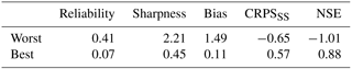
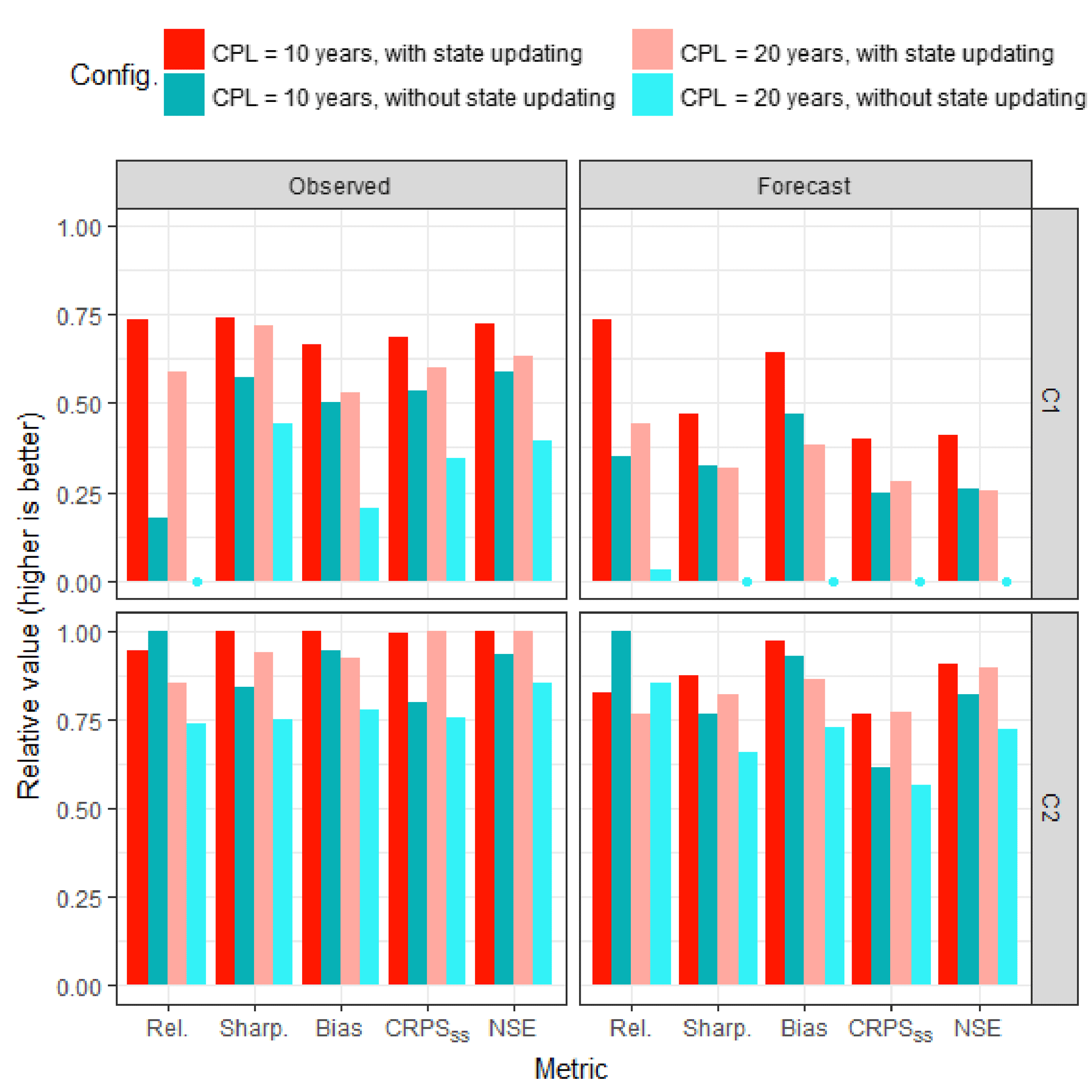
Figure 4 Predictive performance metrics for the two case study catchments (C1 and C2) and the two sources of rainfall forcing data (observed and forecast). Relative metric values are presented (Sect. 3.7 and Table 2); higher values represent better performance. The impact of state updating can be seen by comparing the red versus blue bars. The change in performance due to different calibration period lengths (CPLs) can be seen by comparing the bars with darker versus lighter shading.

4 Results

The performance metrics for all model configurations are summarised in Fig. 4. First the predictive performance of model configurations with and without state updating is compared (Aim 1), and then the influence of calibration period length in the context of catchment non-stationarity is investigated (Aim 2), considering changes in both the predictive performance and changes in CRR parameter values over time.

4.1 Impact of state updating

The impact of state updating on predictive performance can be seen in Fig. 4, by comparing the red and blue bars (darker shading indicating results for the 10-year calibration period length, and lighter shading indicating results for the 20-year calibration period length). It is clear that state updating improves the sharpness, bias, CRPS_SS and NSE metrics.

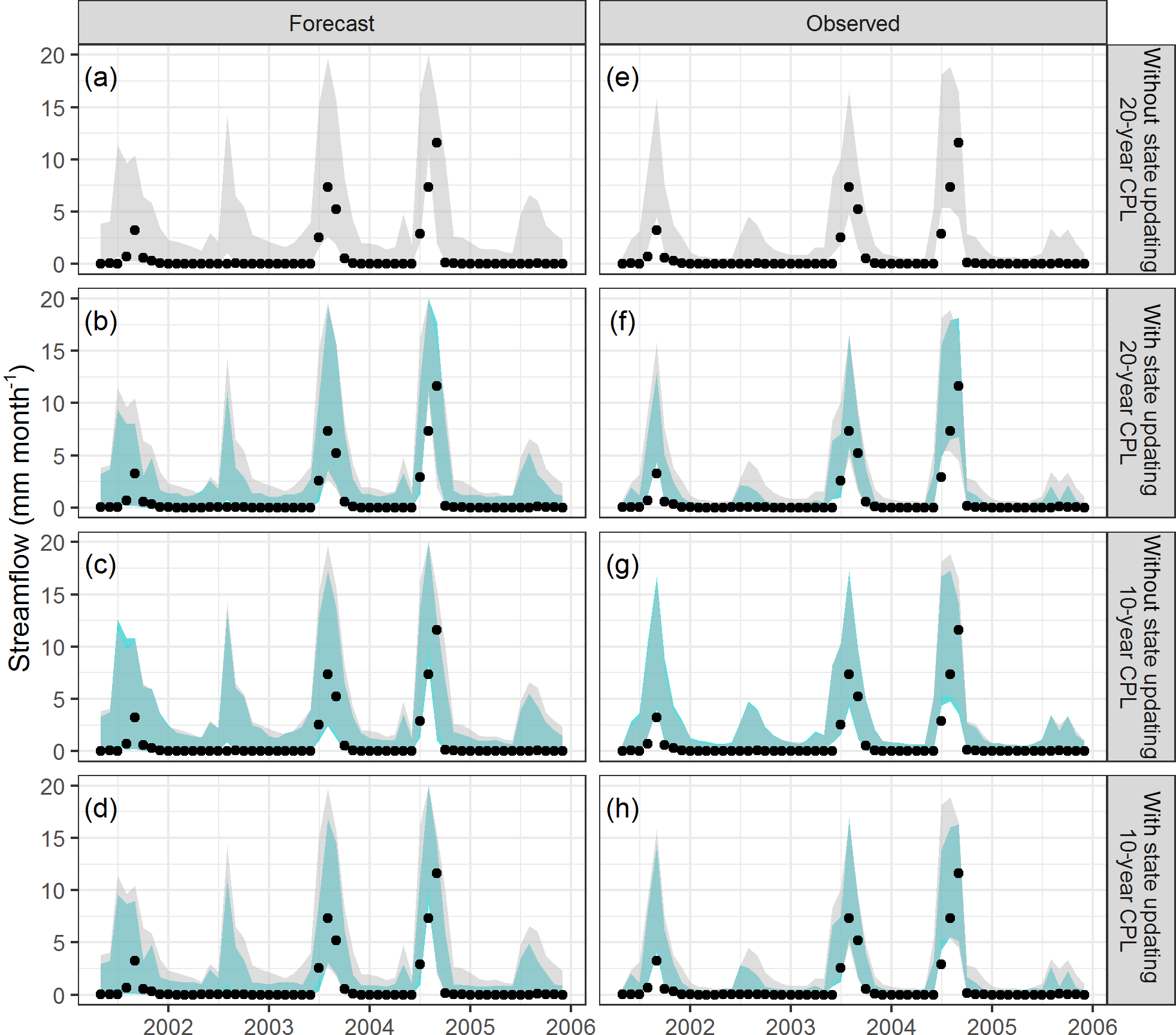
Figure 5 Representative streamflow time series in catchment C1 obtained using forecast rainfall (a, b, c, d) and observed rainfall (e, f, g, h). The shaded area represents the 90th percentile prediction limits and the black dots the observed values. The “traditional approach” of the 20-year calibration period length (CPL) without state updating is shown in grey in each panel.

The improvement in predictive performance achieved by state updating to the observed flow data is tentatively attributed to being able to correct the model for any systematic overestimation of simulated streamflow. Consider Figs. 5 and 6, which show the 90th percentile predictive limits for each model configuration, for catchments C1 and C2, respectively. The longer 20-year calibration period length without state updating is considered the “typical approach”, and is shown in grey in each panel. A representative time period is shown, with the full time series for each case provided in the Supplement. Figures 5 and 6 show that state updating sharpens the predictive limits, especially during low-flow months. For example, this behaviour can be seen for the 20-year CPL by comparing the predictions in panels (a) to (b) for the case of forecast rainfall and the predictions in panels (e) to (f) for the case of observed rainfall.

In terms of reliability, Fig. 4 shows that state updating provides improved predictions for catchment C1. However, for catchment C2, Fig. 4 shows that the reliability of all model configurations is relatively high compared to the reliability achieved in catchment C1, and state updating can lead to a slight loss of reliability.

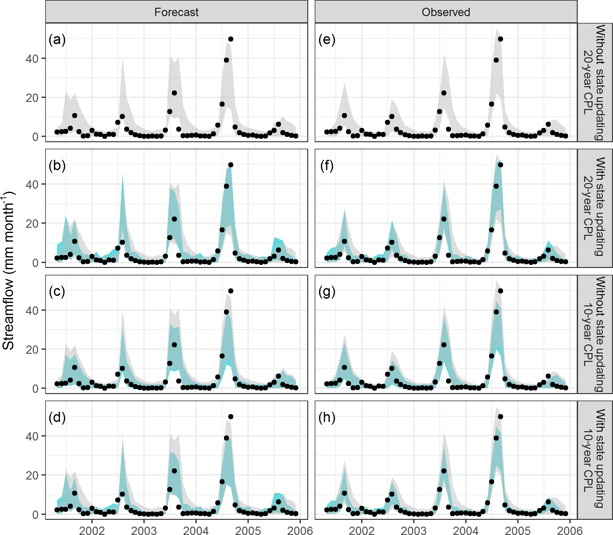
Figure 6 Representative streamflow time series in catchment C2 obtained using forecast rainfall (a, b, c, d) and observed rainfall (e, f, g, h). The shaded area represents the 90th percentile prediction limits and the black dots the observed values. The “traditional approach” of the 20-year calibration period length (CPL) without state updating is shown in grey in each panel.

4.2 Impact of calibration period length

4.2.1 Differences in predictive distribution

The changes in the predictive distribution due to changes in the calibration period length can be seen in Fig. 4, by comparing the darker and lighter shades of each colour (darker colour for 10-year calibration period length, lighter colour for 20-year calibration period length). The following findings can be seen.

• When state updating is not used (comparing dark blue versus light blue in Fig. 4), all metrics improved when the shorter 10-year calibration period length was used.

• When state updating is used (comparing the dark red versus light red in Fig. 4), the impact of the shorter 10-year calibration period length depends on the catchment. In catchment C1, which provided stronger evidence of non-stationarity than catchment C2 (Sect. 2.1), the use of the 10-year calibration period length improves all metrics compared to the use of the 20-year calibration period length. In contrast, in catchment C2, the length of the calibration period had little impact on the NSE and CRPS_SS values, and only small improvements in the reliability, sharpness and bias metrics are obtained when the 10-year period is used.

The differences between the streamflow predictions obtained in the two catchments C1 and C2 (for the case of GR4J forced with observed rainfall) are illustrated in Fig. 7 for the most recent period: 2009–2011. In catchment C1, using a longer calibration period length tends to yield wider prediction limits and an overestimation of the observed flow in 2009 and 2010, whereas using the shorter calibration length provides a better capture of the catchment response in these 2 years. In contrast, in catchment C2, which has less evidence of non-stationarity (Sect. 2.1), the calibration period length makes very little difference to the resulting streamflow predictions.

4.3 Differences in trends in parameter values

Figure 7 Streamflow predictions for catchments C1 (a) and C2 (b) for the period 2009–2011 using observed rainfall. The shaded area represents the 90th percentile prediction limits and the black dots the observed values. For catchment C1, using shorter calibration periods (red) can be seen to produce lower streamflow predictions than using longer calibration periods (blue).

The rolling calibration approach (see Sect. 3.3) enables temporal trends in the parameter distributions to be investigated. Figure 8 presents the median and 90th percentile prediction limits of these distributions for each parameter for each catchment, with the 10-year and 20-year calibration period lengths shown in different colours.

In catchment C1, up until year 2005 (representing models calibrated from 1995 to 2004 for the 10-year calibration period length), the calibration period length has little impact on the median value for each parameter. Slightly wider parameter bounds are obtained when the shorter calibration period length is used, likely due to the reduced data available to infer representative parameter values. Post-2005, the parameter values obtained using the shorter calibration period length respond to the distinct non-stationarity of the catchment discussed in Sect. 2.1. The more pronounced negative values of the groundwater exchange coefficient X2 estimated in the 1994–2005 calibration period are consistent with the reduced runoff ratio in the period post-2000. In contrast, parameter values estimated from the longer calibration period length, which includes data from the 1980s even when predicting the 2000s, do not exhibit this distinct change.

In catchment C2, the median values of parameters estimated from each calibration period length were similar over the record. This result agrees with the lack of strong evidence of non-stationarity in this catchment. However, there is some evidence of a reduction in streamflow in this catchment, with the post-2000 period being characterised by a reduction in the runoff ratio from 0.088 to 0.061 (Sect. 2.1). This reduction is weaker in catchment C2 than in catchment C1, yet appears to be supported by the trends in the median parameter values. Analysis of results from the 20-year calibration period length suggests statistically significant trends (p < 0.05) in the median values of the model parameters, namely ΔX1 = 3.96 and $\mathrm{\Delta }X\mathrm{3}=-\mathrm{5.17}$ mm yr⁻¹. An exception to the pattern of the median parameter values being insensitive to calibration period lengths can be seen in 1999, where the use of the 10-year calibration period length produces higher values of X4 and lower values of X2 and the split introduced in this study (Sect. 3.1). This exception could represent a model fitting anomaly resulting from a shorter calibration period length.

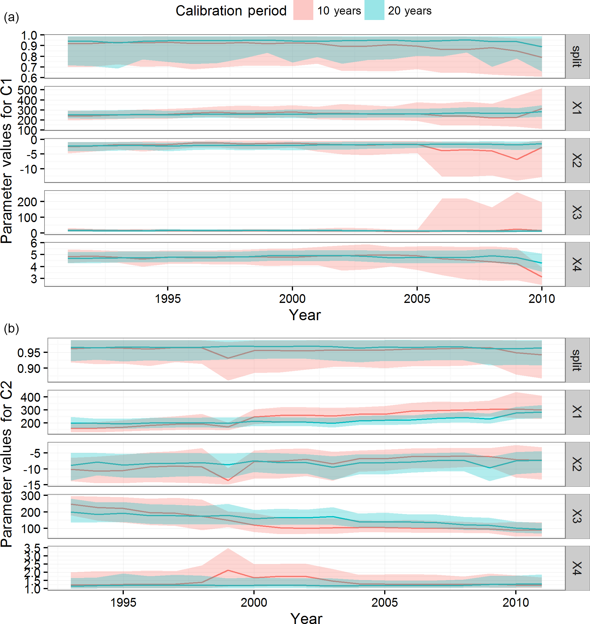
Figure 8 Temporal trends in posterior parameter distributions, for catchments C1 (a) and C2 (b). The median values are shown as the solid lines and the shaded areas represent the 90th percentile prediction limits.

5 Discussion

5.1 Beneficial impact of state updating on forecast performance

Most previous studies have used state updating in a short-term flood forecasting context, and found a limited effect of the initial conditions after a number of days (e.g. Berthet et al., 2009; Randrianasolo et al., 2014; Sun et al., 2017). However, forecasting of flood peak and timing is a different application to the forecasting of streamflow volumes. A number of data-driven modelling studies have demonstrated that monthly streamflow lagged by 1 month (or more) provided some useful information for forecasting at a 1-month lead time (e.g. Bennett et al., 2014; Humphrey et al., 2016; Yang et al., 2017). This study demonstrates that these benefits also hold when CRR models, rather than data-driven approaches, are used as the forecasting model.

State updating is found to improve predictive performance in both catchments considered, for the majority of the multiple performance metrics considered. State updating is expected to reduce predictive bias, as errors in the simulated streamflow during the warm-up period are corrected at the start of the forecast period. State updating is also expected to increase the sharpness of the predictive distribution, as the range of model predictions is generally tightened by forcing the model to simulate the observed streamflow at the start of the forecast period.

The only metric where state updating did not show an improvement is for the reliability of predictions for catchment C2. However, the reliability of all model configurations in this catchment is already relatively high without state updating. All other metrics (sharpness, bias, CRPS and NSE) show improvements from state updating in catchment C2, suggesting potential trade-offs in performance, similar to that found by Crochemore et al. (2016) and McInerney et al. (2017). This slight reduction in reliability is not considered to have a significant detrimental impact on the PD produced for this practical application.

5.2 Importance of choosing a calibration period that is representative of current catchment conditions

Traditionally, long calibration periods are used to maximise the use of available data and increase parameter identifiability. The empirical results in this study suggest that the shorter calibration period can provide better (or at least not worse) predictive performance. The reduction in performance seen when the longer calibration period is used is likely due to the calibration data representing catchment conditions that are substantially different to those in the prediction period. For example, when the prediction period is 2009 (as shown for catchment C1 in Fig. 7), a 20-year calibration period length corresponds to the period of 1989–2008, which includes a large portion of the pre-2000 period when catchment C1 displayed a much higher runoff coefficient (Sect. 2.1). In contrast, a 10-year calibration period length corresponds to a calibration period of 1999–2008, which is likely to be more representative of the lower runoff hydrological regime seen in the post-2000 period.

The reported improvement in model performance with the 10-year calibration period length does not imply that shorter calibration periods would result in further improvements. Shorter calibration period lengths will eventually reduce parameter identifiability (e.g. as manifested by greater parameter uncertainty in Fig. 8), and may produce poor parameter estimates due to fitting only a small number of events and hence being unable to represent the full range of flow conditions.

The empirical findings highlight the benefits of identifying a calibration period of data that is representative of conditions of interest for a given model application, which is a task often overlooked in practical applications. Suitable representative periods can be identified through techniques such as trend analysis, using knowledge of changes in a catchment (e.g. land use data, abstraction volumes), and testing predictive performance for different calibration period lengths (as done in this work). The empirical results indicate that, if the selection of calibration data is poorly implemented, and/or if the modeller naively assumes that longer calibration periods are inherently better for model development, predictive performance can degrade.

5.3 Value of forecasts for improving water management

The forecasting approaches developed in this work can support improved water management in the drainage system considered. The approach currently used by the management authority is very conservative: streamflow forecasts are not attempted, and changes in water management are made only once downstream requirements have been met. With the forecasting models and methods developed in this work, it becomes possible to produce streamflow forecasts with a high reliability, improved sharpness and reduced bias. Thus it becomes possible to provide useful probabilistic estimates of how likely it is that the downstream flow requirements will be met in the next month. With this information, managers can more confidently consider increasing the frequency and duration of inundation for many of the wetlands in the region, and can make decisions on management changes much earlier in the season.

5.4 Future research work

The enhancements to predictive performance of streamflow forecasts from state updating and a shorter calibration period have been demonstrated on two catchments. These catchments were selected based on an established user need for monthly forecasts to improve the water management of a channel drainage system with multiple competing demands. Importantly, the case study catchments in this work are ephemeral and dry, with low runoff ratios. These types of catchments are known to be challenging to model (McInerney et al., 2017; Ye et al., 1997). For example, the models predict a streamflow response in 2002 and 2005 in Fig. 5 that did not occur in the observations, even when observed rainfall and state updating were used. Some of this difference may be due to errors in the input rainfall data, but this result highlights the difficulty in representing streamflow generation in low-yielding, ephemeral catchments, such as those considered. Future work will evaluate the proposed monthly streamflow forecasting techniques over a wider range of catchments and environmental conditions.

6 Conclusions

This work has focused on improving monthly streamflow forecasts by considering two aspects: (1) state updating to force the GR4J hydrological model to match observations from the start of the forecast period, and (2) investigating the trade-offs between using shorter versus longer calibration periods. The analysis was applied to two ephemeral catchments in southern Australia, which are part of a drainage network with competing environmental management demands.

The major findings from the empirical analysis are as follows.

1. State updating improves predictive performance in the case study catchments, for the majority of the multiple performance metrics considered. Previous studies focusing on the forecasting of flood peak and timing have typically found a limited effect of initial conditions on predictive performance after a number of days. This study demonstrates that, when forecasting streamflow volumes, using state updating to more accurately represent initial conditions can have a benefit even at a 1-month lead time.

2. The length of the calibration period has a major impact on the predictive performance of a hydrological model. In the case study catchments, the shorter calibration period typically improves predictive performance, especially in the case study catchment with stronger evidence of non-stationarity. The benefits of a shorter calibration length appear contrary to the standard approach of using as much data as possible for model calibration. The reduction in performance for the longer calibration period is likely due to the model being calibrated to data that represent higher-yielding conditions from the past which no longer hold true in the forecast period. This finding highlights that identifying a data set that is representative of the forecast period, through trend analysis and other knowledge of a catchment, is an important step in model development. If this step is ignored, and it is naively assumed that longer calibration data are inherently better for model development, all aspects of predictive performance may suffer.

The conclusions of this empirical study are limited by the small number of catchments and single hydrological model used. Further work will consider a larger sample of catchments and a wider range of hydrological model structures. In general, we expect the techniques of state updating, post-processing uncertainty estimation, and usage of shorter calibration period length representative of future forecast conditions to be of value to hydrologists and environmental modellers seeking to improve the predictive performance of their modelling systems.