Modeling the changes in water balance components of the highly irrigated western part of Bangladesh

The objectives of the present study were to explore the changes in the water balance components (WBCs) by co-utilizing the discrete wavelet transform (DWT) and different forms of the Mann–Kendall (MK) test and develop a wavelet denoise autoregressive integrated moving average (WD-ARIMA) model for forecasting the WBCs. The results revealed that most of the potential evapotranspiration (P_ET) trends (approximately 73 %) had a decreasing tendency from 1981–1982 to 2012–2013 in the western part of Bangladesh. However, most of the trends (approximately 82 %) were not statistically significant at a 5 % significance level. The actual evapotranspiration (A_ET), annual deficit, and annual surplus also exhibited a similar tendency. The rainfall and temperature exhibited increasing trends. However, the WBCs exhibited an inverse trend, which suggested that the P_ET changes associated with temperature changes could not explain the change in the WBCs. Moreover, the 8-year (D3) and 16-year (D4) periodic components were generally responsible for the trends found in the original WBC data for the study area. The actual data was affected by noise, which resulted in the ARIMA model exhibiting an unsatisfactory performance. Therefore, wavelet denoising of the WBC time series was conducted to improve the performance of the ARIMA model. The quality of the denoising time series data was ensured using relevant statistical analysis. The performance of the WD-ARIMA model was assessed using the Nash–Sutcliffe efficiency (NSE) coefficient and coefficient of determination (R²). The WD-ARIMA model exhibited very good performance, which clearly demonstrated the advantages of denoising the time series data for forecasting the WBCs. The validation results of the model revealed that the forecasted values were very close to actual values, with an acceptable mean percentage error. The residuals also followed a normal distribution. The performance and validation results indicated that models can be used for the short-term forecasting of WBCs. Further studies on different combinations of wavelet analysis are required to develop a superior model for the hydrological forecasting in the context of climate change. The findings of this study can be used to improve water resource management in the highly irrigated western part of Bangladesh.

1 Introduction

The water balance model is considerably important for water resource management, irrigation scheduling, and crop pattern designing (Kang et al., 2003; Valipour, 2012). The model can also be used for the reconstruction of catchment hydrology, climate change impact assessment, and streamflow forecasting (Alley, 1985; Arnall, 1992; Xu and Halldin, 1996; Molden and Sakthivadivel, 1999; Boughton, 2004; Anderson et al., 2006; Healy et al., 2007; Moriarty et al., 2007; Karimi et al., 2013). Therefore, accurately forecasting the water balance components (WBCs) and detecting the changes in them is important for achieving sustainable water resource management. However, hydrometeorological time series are contaminated by noises from hydrophysical processes. This affects the accuracy of the analysis, simulation, and forecasting (Sang et al., 2013; Wang et al., 2014). Hence, denoising the time series is essential for improving the accuracy of the obtained results. In this study, the wavelet denoising technique was coupled with the ARIMA (autoregressive integrated moving average) model for forecasting the WBCs after detecting the changes in them by using different forms of the Mann–Kendall (MK) test. Moreover, the time period responsible for the trends in the WBC time series was identified using discrete wavelet transform (DWT) time series data.

Physics-based numerical models are generally used for understanding a particular hydrological system and forecasting the water balance or water budget components (Fulton et al., 2015; Leta et al., 2016). To achieve reliable forecasting using numerical models, a large amount of hydrological data is required for assigning the physical properties of the grid and model parameters and calibrating the model simulation. However, numerical models have numerous limitations, such as the cost, time, and availability of the data (Yoon et al., 2011; Adamowski and Chan, 2011). Data-based forecasting models and statistical models are suitable alternatives for overcoming these limitations. The most common statistical methods for hydrological forecasting are the ARIMA model and multiple linear regression (Young, 1999; Adamowski, 2007). Many studies have used the ARIMA model to predict water balance input parameters, such as rainfall (Rahman et al., 2016), temperature (Nury et al., 2016), and potential evapotranspiration (P_ET; Valipour, 2012). However, the ARIMA model cannot handle nonstationary hydrological data without preprocessing the input time series data (Tiwari and Chatterjee, 2010; Adamowski and Chan, 2011). Wavelet analysis, a new method in the area of hydrological research, can be used to effectively handle nonstationary data (Adamowski and Chan, 2011). Adamowski and Chan (2011) coupled wavelet analysis with artificial neural network (ANN) models for forecasting hydrological variables, such as the groundwater level, in Quebec, Canada. Kisi (2008), Partal (2010), and Santos and da Silva (2014) developed hybrid wavelet ANN models for monthly and daily streamflow forecasting. Rahman and Hasan (2014) found that the performance of wavelet-based ARIMA models was superior to that of classical ARIMA models for forecasting the humidity of the Rajshahi meteorological station in Bangladesh. A comparative study of wavelet ARIMA models and wavelet ANN models was conducted by Nury et al. (2017). The study indicates that the wavelet ARIMA models are more effective than wavelet ANN models for temperature forecasting. Khalek and Ali (2016) developed the wavelet seasonal ARIMA (W-SARIMA) and wavelet neural network autoregressive (W-NNAR) models for forecasting the groundwater level. They observed that the W-SARIMA model exhibited a superior performance to the W-NNAR model. In all the aforementioned studies, the performance of the wavelet-aided model was better than that of the classical ARIMA and ANN models. Moreover, analyzing the periodicity using wavelet-transformed details and using the approximation components of the hydrometeorological time series data can provide insight regarding the effects of the time period on the data trend (Nalley et al., 2013; Araghi et al., 2015; Pathak et al., 2016). As a result, detecting the periodicity through the wavelet transformation of hydrometeorological time series data has gained popularity in recent years (Partal and Küçük, 2006; Partal, 2009; Nalley et al., 2013; Araghi et al., 2015; Pathak et al., 2016). Studies have been conducted on the spatiotemporal characteristics of hydrometeorological variables, such as rainfall (Shahid and Khairulmaini, 2009; Ahasan et al., 2010; Kamruzzaman et al., 2016a; Rahman and Lateh, 2016; Rahman et al., 2016; Syed and Al Amin, 2016), temperature (Shahid, 2010; Nasher and Uddin, 2013; Rahman, 2016; Syed and Al Amin, 2016; Kamruzzaman et al., 2016a), and P_ET (Hasan et al., 2014; Acharjee, 2017), in Bangladesh. Karim et al. (2012) studied the WBCs, such as the P_ET, A_ET, deficit of water, and surplus of water, of 12 districts in Bangladesh. Kanoua and Merkel (2015) studied the water balance of Titas Upazila (subdistrict) in Bangladesh. Most of the studies conducted on hydrological variables in Bangladesh were limited to detecting trends and forecasting the rainfall and temperature. Therefore, this study was conducted to detect the trends and identify the periodicities in the WBCs, such as the potential evapotranspiration (P_ET), actual evapotranspiration (A_ET), and annual deficit and surplus of water, by co-utilizing the DWT and different forms of the MK test in the western part of Bangladesh. Moreover, a wavelet denoise (WD)-ARIMA model was developed for forecasting the WBCs. To date, no comprehensive study has coupled wavelet denoising methods with ARIMA models for forecasting the WBCs. Wavelet denoising methods are widely used in the engineering and scientific fields. However, these methods have been used to a limited extent in hydrology (Sang, 2013). The combination of wavelet denoising methods with ARIMA models is expected to provide insight regarding WBCs, which would ultimately help policymakers prepare sustainable water resource management plans.

2 Study area, data, and methods

2.1 Study area

The climate of Bangladesh is humid, warm, and tropical. The western part of Bangladesh covers approximately 41 % or 60 165 km² of the country. The geographic coordinates of the study area extend between a latitude of 21^∘36^′–26^∘38^′ N and longitude of 88^∘19^′–91^∘01^′ E. The annual rainfall and average temperature in the study area vary from 1492 to 2766 mm, with an average of 1925 mm, and 24.18 to 26.17 ^∘C, with an average of 25.44 ^∘C, respectively (Kamruzzaman et al., 2016a). Bangladesh is the fourth-largest producer of rice in the world (Scott and Sharma, 2009), and the livelihood of a majority of the people (approximately 75 %) (Shahid and Behrawan, 2008; Kamruzzaman et al., 2016b) depends on agricultural practices. The crop calendar of Bangladesh is related to the climatic seasons. Rice is grown during three seasons (Aus, Aman, and Boro) in Bangladesh. Almost 73.94 % of the cultivable area in the country is used to cultivate Boro rice (Banglapedia, 2003). The Aus and Aman rice varieties are mainly rain-fed crops. However, Boro rice is almost completely groundwater-fed (Ravenscroft et al., 2005) and requires approximately 1 m of water per square meter in Bangladesh (Harvey et al., 2006; Michael and Voss, 2009).

2.2 Data

The national climate database of Bangladesh prepared by the Bangladesh Agricultural Research Council (BARC) was used for this study. The database is available for research and can be obtained from the BARC website (http://climate.barcapps.gov.bd/, last access: 27 July 2018). The database has been prepared from the data recorded by the Bangladesh Meteorological Division and contains long-term monthly climate data, such as rainfall, minimum, maximum, and average temperatures, humidity, sunshine hours, wind speed, and cloud cover. The locations of the meteorological stations in the study area are displayed in Fig. 1. The data are rearranged according to the hydrological year for the period from 1981–1982 to 2012–2013. The hydrological year in Bangladesh begins in April and ends in March.

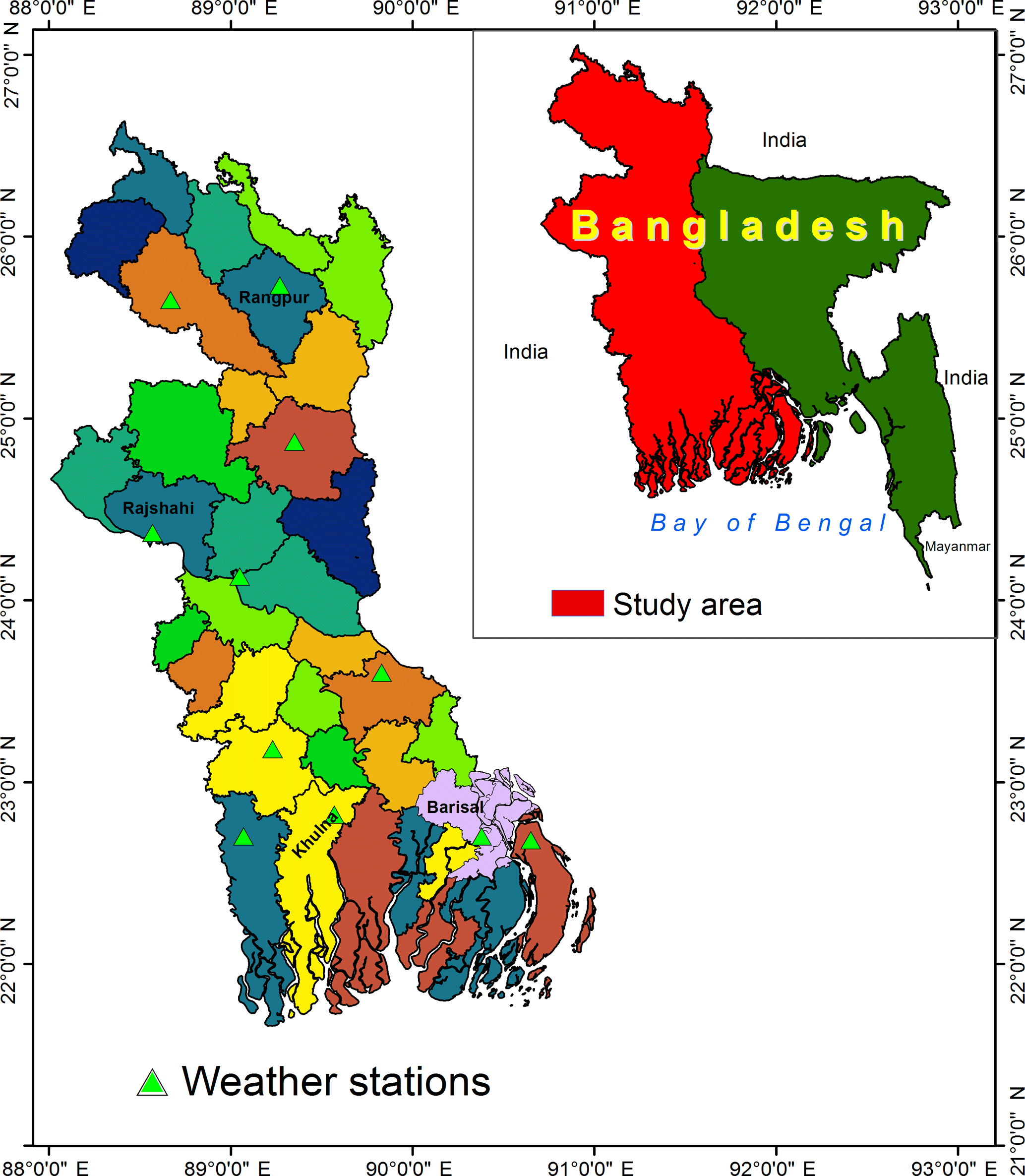
Figure 1 Study area in the western part of Bangladesh with locations of meteorological stations.

2.3 Methods

In this study, the WBCs were calculated and their trends were identified using the MK or Modified MK (MMK) test for evaluating the long-term water balance of the highly irrigated western part of Bangladesh. The DWT data of the WBC time series were analyzed for identifying the time period responsible for the trend in the data. The WBCs were forecasted using the ARIMA model, whose performance was statistically evaluated. If the performance of the model was unsatisfactory for forecasting the WBCs, denoising of the original time series was conducted using DWT techniques to improve the performance of the model. The descriptions of the methods are presented in the following sections.

2.3.1 Calculation of the potential evapotranspiration and water balance components

The potential evapotranspiration (P_ET) is a key parameter to estimate the WBCs. In this study, the potential evapotranspiration was calculated using the Penman–Monteith equation (Allen et al., 1998). The soil–water balance concept proposed by Thornthwaite and Mather (1955) is one of the most widely used methods for estimating the WBCs. This method is suitable for assessing the effectiveness of agricultural water resource management practices and regional water balance studies because it allows the actual evapotranspiration (A_ET), water deficit, and water surplus to be estimated (Chapman and Brown, 1966; Bakundukize et al., 2011; Karim et al., 2012; Viaroli et al., 2017). The actual evapotranspiration (A_ET) is the amount of water removed from the surface due to evaporation and transpiration. The amount by which the P_ET exceeds the A_ET is termed as the deficit. The surplus is the excess rainfall received after the soil has reached its water-holding capacity (de Jong and Bootsma, 1997). Calculating the field capacity of the soil is essential for estimating the WBCs. The field capacity of the soil in the study area was calculated using the soil texture map of Bangladesh prepared by the Soil Resource Development Institute, Bangladesh (SRDI, 1998), where the description of the soils was presented by Huq and Shoaib (2013). The values suggested by Thornthwaite and Mather (1957) for the water-holding capacity of the soil and rooting depth of the plants were used for estimating the WBCs in this study. The first step of the calculation involves subtracting 5 % rainfall from the monthly rainfall data because this amount of water is lost due to direct runoff (Wolock and McCabe, 1999; Karim et al., 2012; Kanoua and Merkel, 2015). The remaining rainfall amount is included in the calculation. The WBCs, such as the A_ET, surplus, and deficit, were estimated using the formulas presented in Table 1. The details of the WBC calculations are available in the Supplement.

Table 1 Calculations of water balance components (Thornthwaite and Mather, 1957).

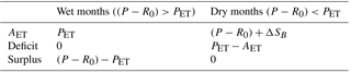
P is the rainfall (mm), R₀ is the direct runoff (mm), P_ET is the potential evapotranspiration (mm), A_ET is the actual evapotranspiration (mm), and ΔS_B is the changes in soil moisture storage (mm).

2.3.2 Trend test

In this study, the trends in the WBCs were detected using the nonparametric MK test (Mann, 1945; Kendall, 1975) because it exhibits a better performance than the parametric test (Nalley et al., 2012) for identifying trends in hydrological variables, such as rainfall (Shahid, 2010), temperature (Kamruzzaman et al., 2016a), P_ET (Kumar et al., 2016), soil moisture (Tabari and Talaee, 2013), runoff (Pathak et al., 2016), groundwater level (Rahman et al., 2016), and water quality (Lutz et al., 2016). The MK test cannot be used to accurately calculate the test statistic (Z) if there exists a significant serial correlation at lag 1 in the time series data (Yue et al., 2002) because the variance is underestimated (Hamed and Rao, 1998). The autocorrelation at lag 1 was checked before analyzing the time series data. If there existed a significant lag-1 autocorrelation at the 5 % level, the MMK test (Hamed and Rao, 1998) was applied instead of the MK test. The estimated Z statistic from the MK or MMK test was evaluated for the direction of the trend (a positive Z statistic indicated an increasing trend and vice versa). Moreover, the Z statistic indicated the level of significance of the obtained trend. If the calculated Z statistic is equal to or higher than the tabulated value of the Z statistic (+1.96), it indicates a significant positive trend at the 95 % confidence level. If the calculated Z statistic is equal to or less than −1.96, it indicates a significant decreasing trend. Moreover, the sequential values of the u(t) statistic derived from the sequential MK (SMK) test (Sneyers, 1990) are used for detecting the change point. The u(t) statistic is similar to the Z statistic (Partal and Küçük, 2006). The magnitude of the change was calculated using Sen's slope estimator (Sen, 1968). Numerous studies have already been conducted (notably Nalley et al., 2012) using the methods described in this section. Further details regarding these methods can be obtained from Mann (1945), Sen (1968), Kendall (1971), Hamed and Rao (1998), Sneyers (1990), and Yue et al. (2002).

2.3.3 Wavelet transform (WT) and periodicity

Wavelet analysis has been used in different parts of the world to identify the periodicity in hydroclimatic time series data (Smith et al., 1998; Azad et al., 2015; Nalley et al., 2012; Araghi et al., 2015; Pathak et al., 2016). WT, a multiresolution analytical approach, can be applied to analyze time series data because it offers flexible window functions that can be changed over time (Nievergelt, 2001; Percival and Walden, 2000). WT can be applied to detect the periodicity in hydroclimatic time series data (Smith et al., 1998; Pišoft et al., 2004; Sang, 2012; Torrence and Compo, 1998; Araghi et al., 2015; Pathak et al., 2016) and exhibits better a performance than traditional approaches (Sang, 2013). There exist two main types of WT, namely continuous WT (CWT) and DWT. Applying the CWT is complex because it produces numerous coefficients (Torrence and Compo, 1998; Araghi et al., 2015), whereas DWT is simple and useful for hydroclimatic analysis (Partal and Küçük, 2006; Nalley et al., 2012). The wavelet coefficients of the DWT with a dyadic format can be calculated as follows (Mallat, 1989):

$$\begin{array}{}\text{(1)}& {\mathit{\psi }}_{m,n}\left({\displaystyle \frac{t-\mathit{\tau }}{s}}\right)=s_o^{-m/\mathrm{2}}\mathit{\psi }\left({\displaystyle \frac{t-n{\mathit{\tau }}_o{s}_o^m}{s_o^m}}\right),\end{array}$$

where ψ is the mother wavelet, m is the wavelet dilation, and n is the wavelet translation. The specified fixed dilation step (s_o) is larger than 1, and τ_o is the location parameter. For practical application, the values of s_o and τ_o are considered as 2 and 1, respectively (Partal and Küçük, 2006; Pathak, 2016). After substituting these values in Eq. (1), the DWT for a time series x_i becomes the following:

$$\begin{array}{}\text{(2)}& W_{m,n}={\mathrm{2}}^{-m/\mathrm{2}}\sum _{i=\mathrm{0}}^{N-\mathrm{1}}{x}_i\mathit{\psi }\left({\mathrm{2}}^{-m}i-n\right),\end{array}$$

where W indicates the wavelet coefficient at a scale s=2^m and location τ=2^mn

In the DWT, details (D) and approximations (A) of the time series can emerge from the original time series after passing through low-pass and high-pass filters, respectively. When approximations are the high-scale and low-frequency components, details are the low-scale and high-frequency components. Successive iterations are performed to decompose the time series into its several low-resolution components (Mallat, 1989; Misiti et al., 1997). In this study, four levels (D1–D4) of decomposition were performed following the dyadic scales. The decompositions are referred to as D1, D2, D3, and D4, which correspond to a 2-, 4-, 8-, and 16-year periodicity, respectively. The Daubechies wavelet was used because of its superior performance in hydrometeorological studies (Nalley et al., 2012, 2013; Ramana et al., 2013; Araghi et al., 2015). To confirm the periodicity present in the time series, the correlation coefficient (Co) between u(t) of the original data, u(t) of the decomposition (D) time series data, and different models (D1 + A … D4 + D3 + A) of the time series data were calculated and the obtained results were compared (Partal and Küçük, 2006; Partal, 2009).

2.3.4 ARIMA models

ARIMA models (Box and Jenkins, 1976) are used in hydrological science to identify the complex patterns in data and project future scenarios (Adamowski and Chan, 2011; Valipour et al., 2013; Nury et al., 2017; Khalek and Ali, 2016). ARIMA models include (1) an autoregressive process (AR) represented by order p, (2) nonseasonal differences for nonstationary data termed as order d, and (3) a moving average (MA) process represented by order q. An ARIMA model of order $(p,d,q)$ can be written as follows:

$$\begin{array}{}\text{(3)}& {\mathrm{\varnothing }}_p\left(L\right){\left(\mathrm{1}-L\right)}^d{Y}_t={\mathit{\theta }}_{\mathrm{0}}+{\mathit{\theta }}_q\left(L\right)U_t,\end{array}$$

where θ₀ is the intercept with a mean of 0, U_t is the white process with constant variance, ∅_p(L) represents the AR term $(\mathrm{1}-{\mathrm{\varnothing }}_{\mathrm{1}}L-\mathrm{\dots }-{\mathrm{\varnothing }}_p{L}^p)$, and θ_q(L) represents the MA term $(\mathrm{1}-{\mathit{\theta }}_{\mathrm{1}}L-\mathrm{\dots }-{\mathit{\theta }}_p{L}^p)$.

2.3.5 Wavelet denoising

Wavelet denoising based on the thresholds introduced by Donoho et al. (1995) has been applied to hydrometeorological analysis (Wang et al., 2005, 2014; Chou, 2011). In this study, the following three analysis steps were performed for denoising the time series data.

1. Decomposing the time series data x(t) into M resolution levels for obtaining the detail coefficients (W_j,k) and approximation coefficients using the DWT.

2. The detail coefficients obtained from the DWT (1 to M levels) were treated using threshold (T_j) selection. A soft or hard threshold can be used to deal with detail coefficients and obtain the decomposed coefficient. In this study, a soft threshold was selected because it performed better than a hard threshold (Wang et al., 2014; Chou, 2011).

   $$\begin{array}{ll}{\displaystyle }& {\displaystyle }\text{Soft threshold processing:}\\ {\displaystyle }& {\displaystyle }W{{}^{\prime }}_{j,k}=\left\{\begin{array}{ll}\mathrm{sgn}\left(W_{j,k}\right)\left(\left|W_{j,k}\right|-T_j\right)& \left|W_{j,k}\right|>T_j\\ \mathrm{0}& \left|W_{j,k}\right|<T_j\end{array}\right..\end{array}$$

3. Detail coefficients from levels 1 to M and approximate coefficients at level M were reconstructed to obtain denoising time series data.

Selecting the threshold value is essential for denoising the data. In this study, the universal threshold (UT) method (Donoho and Johnstone, 1994) was used for estimating the threshold value because it exhibited satisfactory performance in analyzing hydrometeorological data (Wang et al., 2005; Chou, 2011).

2.3.6 Assessment of model performance

There exist several indicators to assess the performance of the models. The Nash–Sutcliffe efficiency (NSE) (Nash and Sutcliffe, 1970) coefficient, a normalized goodness-of-fit statistic, is the most powerful and popular method for measuring the performance of hydrological models (McCuen et al., 2006; Moussa, 2010; Ritter and Muñoz-Carpena, 2013). The NSE coefficient was used in this study to evaluate and compare the ARIMA and WD-ARIMA models. The NSE is calculated as follows (Nash and Sutcliffe, 1970):

$$\begin{array}{}\text{(4)}& \mathrm{NSE}=\mathrm{1}-{\displaystyle \frac{{\sum }_{i=\mathrm{1}}^N(O_i-P_i{)}^{\mathrm{2}}}{{\sum }_{i=\mathrm{1}}^N(O_i-\stackrel{\mathrm{‾}}{O}{)}^{\mathrm{2}}}}=\mathrm{1}-{\left({\displaystyle \frac{\mathrm{RMSE}}{\mathrm{SD}}}\right)}^{\mathrm{2}},\end{array}$$

where N, O_i, P_i, $\stackrel{\mathrm{‾}}{O}$, and SD are the sample size, number of observations, model estimates, mean, and standard deviation of the observed values, respectively. The performance of a model can be evaluated according to its NSE value as very good (NSE≥0.9), good (NSE = 0.8–0.9), acceptable (NSE≥0.65), and unsatisfactory (NSE < 0.65) (Ritter and Muñoz-Carpena, 2013). E_RMS is the root-mean-square error and can be calculated as follows:

$$\begin{array}{}\text{(5)}& E_{\mathrm{RMS}}=\sqrt{{\displaystyle \frac{{\sum }_{i=\mathrm{1}}^N(O_i-P_i{)}^{\mathrm{2}}}{N}}}.\end{array}$$

The coefficient of determination (R²) is another goodness-of-fit test to measure the performance of models. The perfect fit of the model draws a line between the actual values and fitted values, where R² is 1. If y_i is the observation data, ${\widehat{y}}_i$ represents the model-forecasted values of y_i and N is the number of data points used. R² is given as follows (Sreekanth et al., 2009):

$$\begin{array}{}\text{(6)}& R^{\mathrm{2}}=\mathrm{1}-{\displaystyle \frac{{\sum }_{i=\mathrm{1}}^N{\left(y_i-{\widehat{y}}_i\right)}^{\mathrm{2}}}{{\sum }_{i=\mathrm{1}}^N{\left(y_i\right)}^{\mathrm{2}}-\frac{({\sum }_{i=\mathrm{1}}^N{y}_i{)}^{\mathrm{2}}}{N}}}.\end{array}$$

Moreover, the mean percentage error (E_MP) and mean error (E_M) were also calculated to evaluate the validation of the model for forecasting. E_MP indicates the percentage of bias (large or small) between the forecasted and actual data (Khalek and Ali, 2016). E_MP and E_M can be calculated as follows:

$$\begin{array}{}\text{(7)}& {\displaystyle }& {\displaystyle }{E}_{\mathrm{MP}}=\left({\displaystyle \frac{\mathrm{1}}{n}}\sum _{t=\mathrm{1}}^n{\displaystyle \frac{Y_t\left(\mathrm{actual}\right)-Y_t\left(\mathrm{forecasted}\right)}{Y_t\left(\mathrm{actual}\right)}}\right)\times \mathrm{100}\mathit{\%},\text{(8)}& {\displaystyle }& {\displaystyle }{E}_{\mathrm{M}}={\displaystyle \frac{\mathrm{1}}{n}}\sum _{t=\mathrm{1}}^n[Y_t\left(\mathrm{actual}\right)-Y_t(\mathrm{forecasted}){]}^{\mathrm{2}}.\end{array}$$

3 Results

3.1 Exploratory statistics of the water balance components

The mean annual P_ET in the study area between 1981–1982 and 2012–2013 varied from 1228 to 1460 mm (Fig. 2a), with an average of 1338 mm. High P_ET values were observed in the central part of the area, where the annual rainfall was low, but the temperature was high (Kamruzzaman et al., 2016a). The standard deviations of the P_ET varied from 205 (Jessore station) to 41 mm (Bhola station). The A_ET (Fig. 2b) (average = 925 mm) was almost 31 % less than the P_ET because during the dry months (December–May), the soil moisture condition reached a critical stage. The annual surplus of water varied from 515 to 1277 mm (Fig. 2c), with an average of 838 mm. According to Wolock and McCabe (1999), 50 % of the surplus water can be considered as runoff for the major parts of the world. A high amount of surplus water was found in the northern part of the study area and along the coastal area. The annual deficit of water, which mainly occurred during the dry season (December–May), varied from 329 to 556 mm, with an average of 416 mm (Fig. 2d). The highest annual deficit of water was observed in Rajshahi, which is located in the central–western part of the study area, where the depth of groundwater below the surface increases rapidly (Shamsudduha et al., 2009; Rahman et al., 2016).

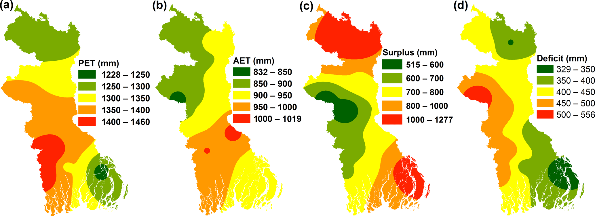
Figure 2 Distribution of mean annual (a) P_ET, (b) A_ET, (c) surplus, and (d) deficit of water in the study area during the hydrologic year 1981–1982 to 2012–2013.

3.2 Trend and periodicity of the water balance components

3.2.1 Potential evapotranspiration

The MK or MMK test based on lag-1 autocorrelation was applied to detect the trend in the P_ET. Table 2 represents the Z statistic of the MK or MMK test for the original P_ET time series data and the Z statistic of the decomposition (D1–D4), approximation (A), and model (D1 + A … D3 + D4 + A) time series. The estimated Z statistic of the original data ranged from −2.07 (Satkhira station) to 2.37 (Bhola station). The Satkhira and Bhola stations exhibited significant P_ET trends. The plots of the sequential u(t) statistic obtained from the SMK test for these two stations are displayed in Fig. 3, where the dashed lines correspond to a 5 % significance level (±1.96). The decreasing P_ET trend for the Satkhira station began in 1985–1886, and a significant decreasing trend occurred in 1993–1994. The trend reversed after 2007–2008. However, the significant increasing P_ET trend of the Bhola station began very recently (2010–2011) after some fluctuation.

Table 2 Z statistic of MK or MMK of original time series, approximation, and different models P_ET of DWT (the dominant components are shown in bold and the asterisks denote significance at a 5 % level).

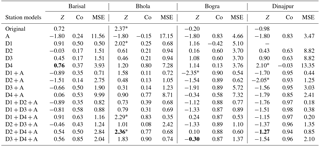
MSE, total mean square error; Co, correlation between original data and DWT models.

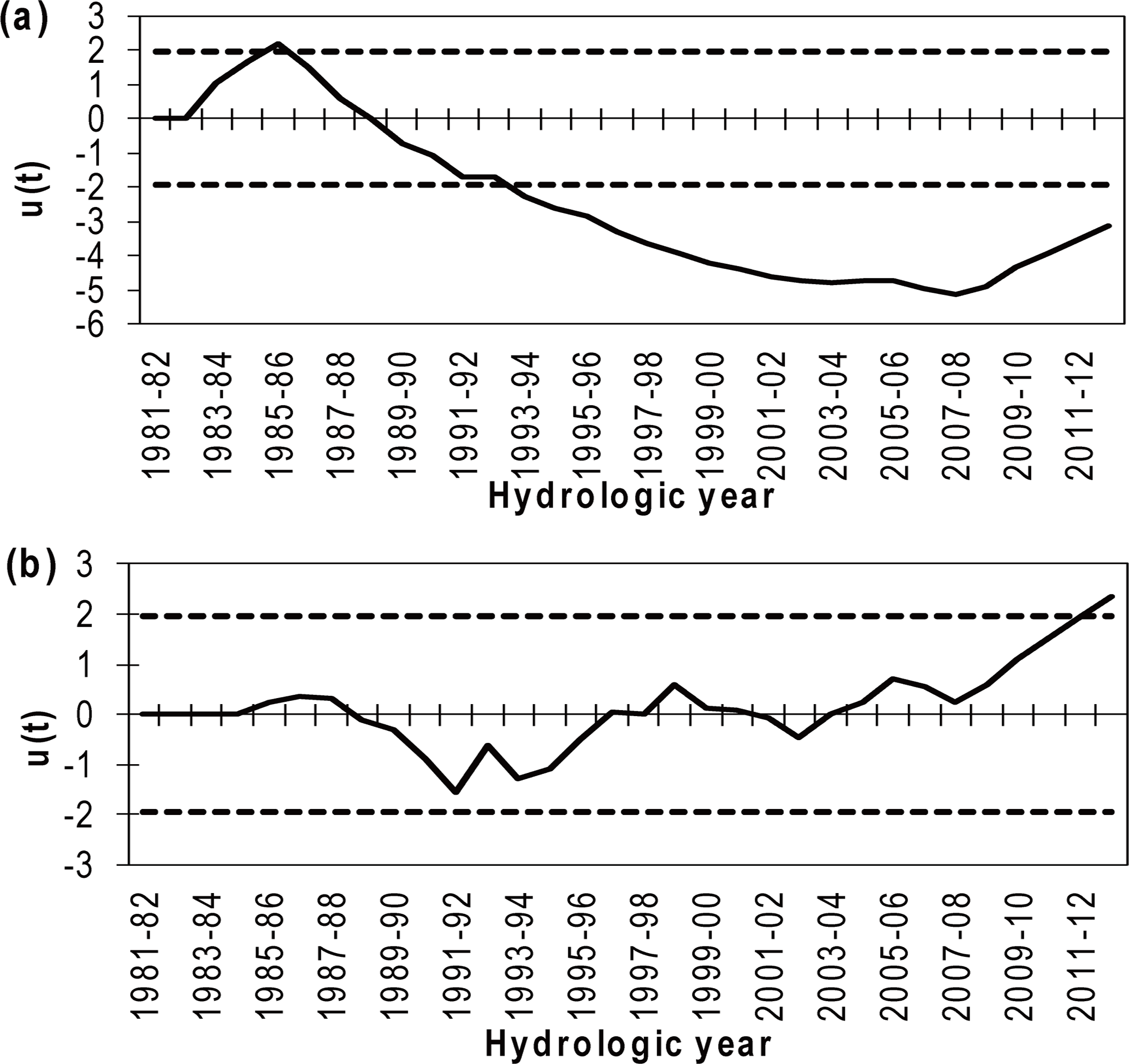
Figure 3 Sequential values of the u(t) statistics of (a) Satkhira station and (b) Bhola station.

Most of the trends (73 %) observed in the P_ET time series data of the study area were negative and statistically insignificant at the 95 % confidence level or 5 % significance level. Moreover, the Z statistic of the approximation (A) time series obtained using the DWT indicated decreasing P_ET trends for all the stations. The calculated Z statistic of the approximation (A) time series was approximately −1.8 after rounding the figures for all the stations. The approximation time series data of all the stations exhibited a similar pattern (Fig. S1 of the Supplement) over time. The magnitude of P_ET changes ranged from −10.89 mm yr⁻¹ for the Satkhira station to 1.67 mm yr⁻¹ for the Bhola station (Fig. 4a). The MK or MMK test was also applied to the decomposition time series and model time series generated from the combination of the approximation and decomposition time series data. Table 2 represents the results for four stations arranged in alphabetical order, and the complete results can be found in Table S1 of the Supplement. To determine the dominant periodicity affecting the P_ET trends, a two-step analysis was performed. First, the value closest to the Z statistic of the original time series data was obtained from the Z-statistic values of different model and decomposition time series data. Second, the correlation coefficients (Co) of pairs of data (such as the Co between the u(t) statistics obtained from the SMK test for the original and decomposition time series data) were estimated, and the highest Co was determined from the estimated Co values for different pairs (Table 2). The Z statistic of the D4 time series data for the Barisal station was 0.76, which was the closest to the Z statistic (0.72) of the original time series data (Table 2). Moreover, the Z statistic of the model (D3 + D4 + A) time series data was 0.56, which is the second-nearest value to the Z statistic of the original time series and has the highest correlation coefficient (Co = 0.85). The D4 (16-year) component was the dominant periodic component in the trend of the original data. However, D3 also affected the trend of the data. The Z-statistic value (2.47) of the original time series for the Bhola station was the closest to that (2.36) of the model (D2 + D4 + A) time series data. However, the Z-statistic values of the D2, D4, D2 + A, and D4 + A time series were 0.61, 1.2, 0.48, and 0.9, respectively. These values were not close to the Z statistic of the original time series data. Hence, in this case, the Z statistic was unable to determine which periodic component (D2∕D4) was the basic periodic component for the significant trend in the original data. To determine the dominant periodic component, the values of Co were analyzed. The correlation coefficient (Co) between the u(t) statistic of the SMK test for the original and D4 time series data was higher than the correlation coefficient between the u(t) statistic of the SMK test for the original and D2 time series data (Table 2). Moreover, the values of the Z statistic for time series with the D4 components, such as the D4 and D4 + A model time series, were higher than those for time series with the D2 component (D2 and D2 + A) (Table 2). Therefore, D4 was the main periodic component responsible for the P_ET trend of the Bhola station. However, the Z-statistic values of D4 and D4 + A were not close to the Z statistic of the original data (Table 2). Moreover, there existed a statistically significant positive trend in the original P_ET data of the Bhola station, whereas the trends of the D4 and D4 + A model time series data were not statistically significant. When the D2 time series was added to the D4 + A model time series data, the Z statistic of the resultant (D2 + D4 + A) model time series data was very close to that of the original time series data. The trend of the D2 + D4 + A model time series was statistically significant, similar to the trend in the original time series data (Table 2). Hence, D2 affected the trend of the original time series data. Station-wise analysis indicated that almost half of the stations exhibited harmony between the Z-statistic values of the D3 + D4 + A model and original time series data. Individual analysis of the D3 and D4 time series data indicated that a higher relationship existed between the D4 and original time series data. Three stations (Dinajpur, Ishurdi, and Jessore) exhibited similar Z-statistic values for the original and D1 + D4 + A model time series data, with higher Co values of the u(t) statistic for the SMK test on the D4 time series data than that for the SMK test on the original data (except for the Ishurdi station). Moreover, two stations (Bhola and Satkhira) exhibited significant trends in the original data. The closest Z statistic was found between the original and D2 + D4 + A time series data for both of the stations. D4 (16-year periodicity) was the dominant periodic component according to the Co values for both these stations. Therefore, 16-year periodicity was the main periodic component responsible for the trends in the P_ET data over the study area. Moreover, D3 (8-year) periodicity also had an effect on the trends for some stations (Tables 2 and S1). D4 (16-year) periodicity dominates the annual rainfall trend for the Marmara region in Turkey (Partal and Küçük, 2006). Araghi et al. (2015) determined that 8–16-year (D3 to D4) periodicity is responsible for the trends in the annual temperature in Iran.

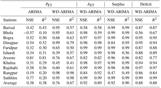
Table 3 Comparison of performance of ARIMA model and WD-ARIMA model.

3.2.2 Actual evapotranspiration

All the stations except the Bogra station exhibited decreasing trends in the A_ET. The calculated Z statistic ranged from −2.90 for the Bogra station to 0.31 for the Ishurdi station. Similar to the P_ET trends, the A_ET trends were also insignificant at a 5 % significance level. However, the Ishurdi station exhibited a significant (at a 5 % significance level) decreasing trend. The magnitudes of the trends of the original A_ET data varied from −5 mm yr⁻¹ for the Faridpur station to 0.75 mm yr⁻¹ for the Bogra station. The distribution of the trend magnitude is displayed in Fig. 4b. The periodicity in the A_ET was marginally different from that in the P_ET (Table S2). For almost half of the stations (five), D2 (4-year) was the main periodic component. D4 (16-year) also affected the trend because the Z statistic of the D2 + D4 + A model time series was the nearest to that of the original series for the Khulna and Ishurdi stations. Moreover, D4 (16-year) was the main periodic component for the Rangpur and Rajshahi stations. D1 (2-year) was the dominant periodic component for the Barisal, Bhola, and Bogra stations. The A_ET value depends on climatic factors, such as the P_ET, rainfall, and soil moisture conditions. The variations in the periodicities of the A_ET and P_ET were mainly related to the soil moisture conditions of the area.

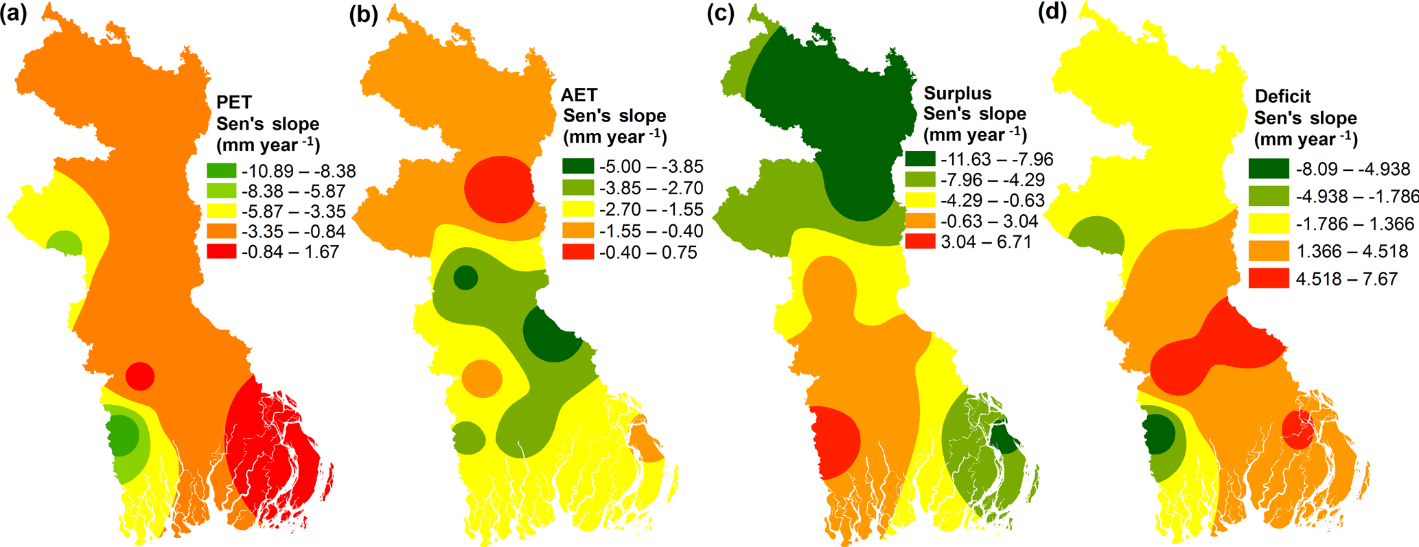
Figure 4 Distribution of rate of changes of WBCs during the period of 1981–1982 to 2012–2013.

3.2.3 Surplus

Almost 82 % of the stations exhibited insignificant decreasing trends for the annual surplus of water. The magnitude of the trends of the original annual surplus data ranged from −11.63 to 6.71 mm yr⁻¹ (Fig. 4c). The periodicity characteristics of the P_ET and surplus were similar (Table S3). D4 (16-year) was the main periodic component present in seven stations. In most cases, D2 was also present (D2 + D4 + A), except in Rajshahi. D3 (8-year) was mainly responsible for the surplus trend of three stations. Surplus mainly occurred during the rainy season (June–October) in the study area, when the soil pores were almost completely filled with water and the A_ET was equal to the P_ET. Surplus mainly depends on rainfall and hence provides insight regarding the periodicity in rainfall.

3.2.4 Deficit

Approximately 73 % of the stations exhibited increasing trends for the annual deficit of water. The increasing trends were significant for two stations at the 95 % confidence level (Table S4). However, the Satkhira station exhibited a significant decreasing trend (Z $=-$2.08) in the annual deficit of water. The magnitude of the trends of the original annual deficit data ranged from −8.1 to 7.7 mm yr⁻¹ (Fig. 4b). Periodicity analysis revealed that D4 was mainly responsible for the trends in the annual deficit of water. The Z statistic of the (D2 + D4 + A) model time series data was close to the Z statistic of the original time series data (Table S4). D3 (8-year periodicity) was also responsible for the trends in the data of the two stations.

3.3 Model selection and forecasting ability

The ARIMA model was selected for forecasting the WBC time series. A four-step analysis was performed during time series modeling. (1) First, the stationarity of the data was checked using the Augmented Dickey–Fuller (ADF) test. (2) Then, the autocorrelation function (ACF) was used for selecting the order of the MA process (Figs. S2–S5). (3) The partial autocorrelation function (PACF) was then used for selecting the order of the AR process (Figs. S2–S5). (4) Finally, the appropriate model was selected based on several trials and model selection criteria, such as Akaike information criterion (AIC) and Bayesian information criterion (BIC). In addition to the manual model selection based on the ACF, PACF, AIC, and BIC, the auto ARIMA function of the “forecast” package (Hyndman et al., 2017) of R (R 3.4.0 language developed by R Core Team, 2016) was used during the trails for model selection to obtain information regarding the nature of the data for modeling. The model with the lowest AIC and BIC values and highest R² value was selected. The Q–Q plot was prepared to examine the normality of the residuals. The performance of the ARIMA model (parameters are given in Table S5) was evaluated using the NSE coefficient and R² values (Table 3). The estimated NSE coefficient of the ARIMA model for the P_ET time series varied from −0.6 for the Bhola station to 0.81 for the Jessore station (Table 3). The ARIMA model exhibited an unsatisfactory performance for almost all the stations. The average NSE coefficient of the 11 stations was 0.38, and the R² values ranged from 0.1 to 0.81, with an average of 0.38. Moreover, the NSE coefficient of the Bhola station indicated that the ARIMA model was unsuitable for forecasting the P_ET. The ARIMA model was also applied to the A_ET, surplus, and deficit time series data. There existed no significant spikes in the ACF and PACF of the A_ET (Fig. S3). Moreover, the results obtained from the auto ARIMA functions exhibited similar results. Therefore, the ARIMA model was unsatisfactory for forecasting the variability in the A_ET. For WBCs such as surplus and deficit, the performance of the ARIMA model was similar to that of the A_ET, except for a few cases. Because hydrometeorological data are affected by noises from different hydrophysical processes (Wang et al., 2014), the results obtained using the ARIMA models were unsatisfactory. To improve model performance, noise must be removed from the data. In this study, DWT denoising was applied to the WBC data and the quality of the denoising time series data was examined before further processing. When selecting a method for denoising the time series using WT, the mean of the original and denoising time series data should be close and the standard deviation of the denoising time series should be less than that of the original time series (Wang et al., 2014). Figure 5a displays the means of the actual and wavelet denoising P_ET time series. No visible difference was observed between the mean of the original and DWT wavelet denoising time series data. Moreover, the standard deviation of the P_ET for the wavelet denoising time series was lower than that for the original time series (Fig. 5b). The A_ET, surplus, and deficit time series also exhibited similar results. Furthermore, the lag-1 autocorrelation of the wavelet denoising time series data must be higher than that of the original time series (Wang et al., 2014). Under this condition, the absolute lag-1 value of autocorrelation for the wavelet denoising time series was higher than that for the original series (Figs. S2b, S3b, S4b, and S5b). The performance of the WD-ARIMA model is represented in Table 3. After denoising the data, the performance of the ARIMA model was satisfactory for all the WBC time series data (Table 3). The average NSE coefficient of the WD-ARIMA model for the P_ET time series of the 11 stations located in the western part of Bangladesh was 0.76, with an average R² value of 0.67. The R² and NSE coefficient values indicated that the performance of the WD-ARIMA model was better than that of the classical ARIMA model for the modeling of P_ET (Table 3). Moreover, the average NSE value of the WD-ARIMA model for the A_ET time series of the 11 stations was 0.92, which indicated that the performance of the model was very good. The average R² value was 0.89, which indicated that the model could explain almost 89 % of the variance in the data (Table 3). The WD-ARIMA model also exhibited a very good forecasting performance for the annual surplus and deficit (Table 3). The average NSE coefficient of the WD-ARIMA model for the annual surplus of the 11 stations was approximately 0.92, and the average R² value was 0.9. The WD-ARIMA model exhibited a good performance in forecasting the annual deficit (average NSE = 0.88). The performance of the WD-ARIMA model was good or very good for forecasting the A_ET, annual surplus, and annual deficit. However, the performance was acceptable for forecasting the P_ET. This deviation may have arisen because the variability of the P_ET was higher than that of the other WBCs or the deviation may be related to the variability of climatic variables.

Figure 5 Comparison between actual and wavelet denoise P_ET time series (a) mean and (b) standard deviation.

The WD-ARIMA models were validated to explore their forecasting ability. The mean percentage error (E_MP) of the forecasted values for the 4-year period from 2008–2009 to 2012–2013 was calculated to determine the percentage bias of the forecasted data (Table 4). The average E_MP of the WD-ARIMA model for the P_ET values of the 11 stations was −0.6 (ranging from 0.75 to −3.34), which indicated that the forecasted values were marginally lower than the actual values. The typical plots of the actual time series data versus the fitted model data, normal Q–Q plots of the residuals of the models, and actual and observed values for the WBCs (plots for all the stations are displayed in Figs. S6–S9) are illustrated in Fig. 6. The plot of the actual values versus the forecasted values (Fig. 6) indicates that the actual and forecasted values were very close for the hydrologic years 2009–2010 and 2010–2011. The normal Q–Q plots revealed that the residuals of the models were near normal. However, the differences in the values increased after these two hydrologic years for all the WBCs (Figs. S6–S9). The E_MP values of WD-ARIMA models for the A_ET ranged from −0.7 to 0.2, with an average of −0.09, which indicated that the forecasted A_ET values were marginally lower than the actual A_ET values. The E_MP values for the annual surplus (average $=-$0.75) and annual deficit (average $=-$0.12) were similar to that for the A_ET and P_ET. The average E_MP values for all the WBCs were negative, which indicated that the forecasted values for the WBCs were marginally lower than the actual values for most of the stations.

Table 4 Accuracy of WD-ARIMA models of WBCs for validation of the model's predictive ability for the period of 2009–2010 to 2012–2013.

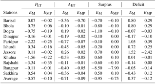
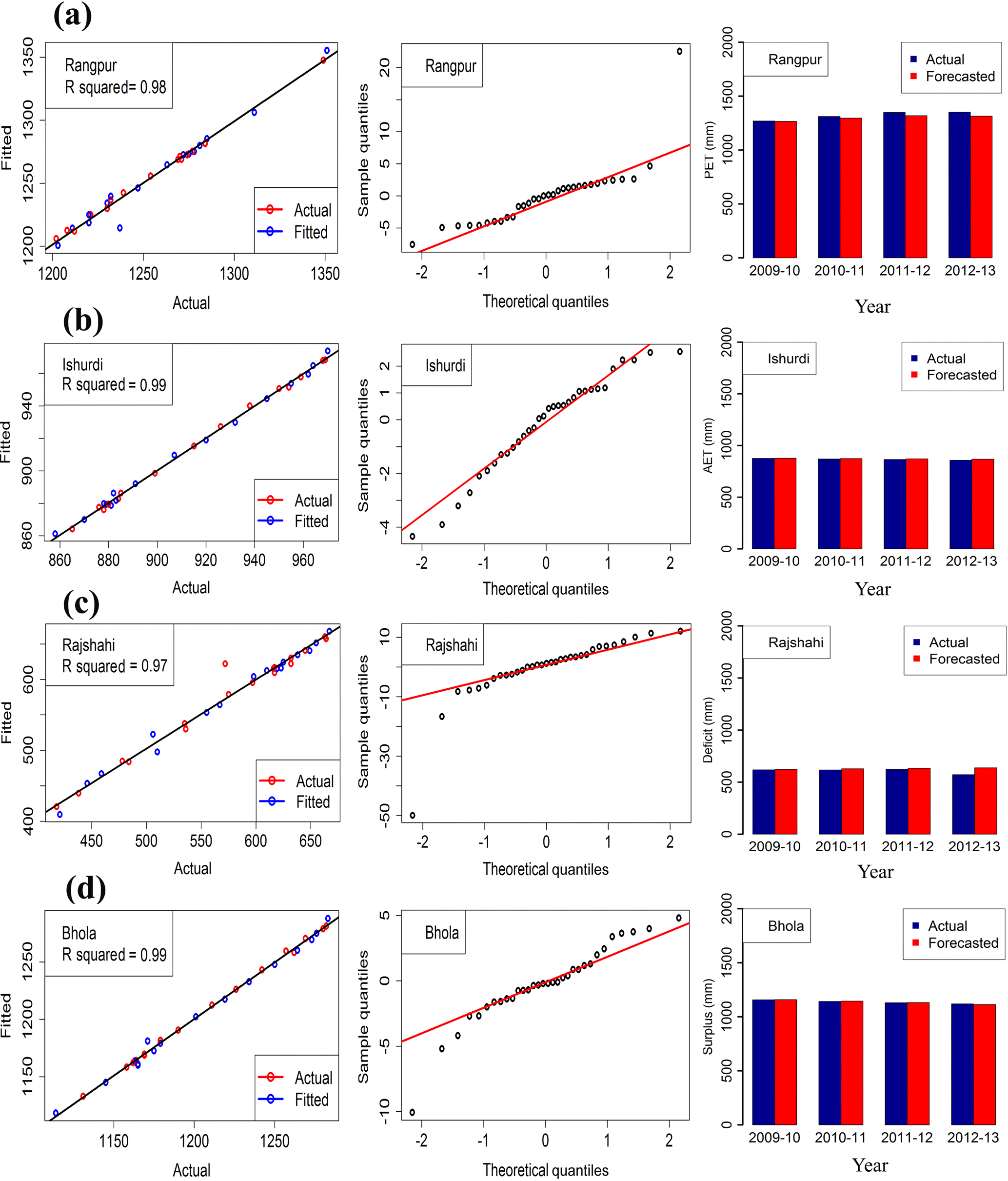
Figure 6 Plot of best WD-ARIMA model first panel represents actual versus fitted values for the period of 1981–1982 to 2012–2013, the second panel is normal Q–Q plot of residuals of the model, and the third panel shows actual, fitted, and forecasted values for 2009–2010 to 2012–2013. (a) P_ET of Rangpur station located in the north, (b) A_ET of Ishurdi station located in the central part, (c) deficit of Rajshahi station located in NW Bangladesh, and (d) surplus of Bhola station located in the south of the study area.

3.4 Discussion

This study indicated that a decreasing P_ET trend dominated the study area. However, positive trends in the rainfall and temperature dominated the western part of Bangladesh (Shahid and Khairulmaini, 2009; Kamruzzaman et al., 2016a). Moreover, a recent study found a negative trend in the evapotranspiration for four stations located in northwest Bangladesh (Acharjee et al., 2017). Although the annual rainfall and temperature of the Satkhira station exhibited positive trends (Kamruzzaman et al., 2016a), its P_ET exhibited a significant decreasing trend. Increasing temperature and decreasing P_ET trends were observed in the Yunnan Province of South China (Fan and Thomas, 2012). McVicar et al. (2012) also found decreasing P_ET trends in different parts of the world. Therefore, although the temperature is the primary factor driving changes in the P_ET (IPCC, 2007), temperature-based models cannot suitably explain the causes of P_ET changes. To obtain a detailed insight regarding the mechanisms underlying the P_ET changes, a detailed analysis must be conducted of all climatic variables, such as rainfall, temperature, sunshine hours, wind speed, and humidity, and climate-controlling phenomena, such as El Niño–Southern Oscillation.

The WD-ARIMA model was used in this study for forecasting the WBCs. The performance of the model indicated the benefit of denoising hydrological time series data, such as the P_ET, A_ET, surplus, and deficit. However, the NSE coefficient indicated that the performance of the model was acceptable for P_ET forecasting (NSE ≥ 0.65). The deviation between the forecasted values and actual values increased with increasing time steps. Therefore, the WD-ARIMA model was unsuitable for long-term forecasting. The WD-ARIMA model was developed by coupling the discrete wavelet denoising time series data and ARIMA model. The soft threshold method was selected for denoising the time series data, and the UT method was used for determining the threshold value. However, there exist other approaches, such as SURE (Stein, 1981) and MINMAX (Donoho and Johnstone, 1998), for determining the threshold value. Moreover, Wang et al. (2014) developed a hybrid method called the adaptive wavelet denoising approach using sample entropy (AWDA-SE) for denoising hydrometeorological time series data, such as rainfall and streamflow data. The study (Wang et al., 2014) indicated that the performance of the developed denoising method was better than that of conventional methods for denoising rainfall and streamflow data. The aforementioned approaches may be used to increase the performance of the ARIMA model for forecasting hydrological variables, such as the P_ET. Moreover, there exist several mother wavelet families, such as Daubechies, Haar, Coiflets, Morlet, and Mexican hat (Sang, 2013). In this study, only Daubechies 6 from the Daubechies wavelet family was applied as the mother wavelet for the DWT. The WD-ARIMA model exhibited very good performance for forecasting the A_ET, surplus, and deficit, whereas the classical ARIMA model exhibited poor performance or was unable to forecast the WBCs. Moreover, studies (Chou, 2011; Kisi, 2008; Partal, 2009; Santos and da Silva, 2014; Rahman and Hasan, 2014; Nury et al., 2016; Adamowski and Chan, 2011; Khalek and Ali, 2016) have indicated that the performance of wavelet-aided models is better than that of the classical ARIMA and ANN models for forecasting nonstationary hydrometeorological variables. Because traditional methods such as Wiener filtering, Kalman filtering, and Fourier transform are unsuitable for nonstationary hydrological time series data (Adamowski and Chan, 2011; Sang, 2013), wavelet denoising can be used to improve the performance of the classical ARIMA model for forecasting hydrological variables.

4 Summary and conclusions

In this study, the changes in the WBCs were explored using various forms of the wavelet-aided MK test. Moreover, a wavelet-aided ARIMA model was used for forecasting the WBCs. The results obtained from trend analysis indicated that decreasing trends were dominant in all the WBCs in the western part of Bangladesh during the period from 1982–1983 to 2012–2013. However, most of the trends were insignificant at the 95 % confidence level. One significant positive and one significant negative P_ET trend was found for the Satkhira and Bhola stations, respectively. Different combinations of the D and A (i.e., D + A and D + A + A) components of the DWT were analyzed using the Co value of the u(t) statistic from the SMK test, which provides detailed information regarding the dominant periodicity and time period affecting the trend of the original data (see the Trend and periodicity section or the example of the Bhola station). The findings of this study revealed that to obtain details regarding the time period responsible for the trends in the data, different combinations of components (D + A and D + A + A) must be analyzed rather than only the details (D) or approximation (A) components of the WT data. Moreover, this study indicated that the changes in temperature and rainfall were not only associated with the changes in the P_ET. To determine the attributes of P_ET changes, a detailed analysis must be conducted of all the relevant climatic variables. In the western part of Bangladesh, the D3 (8-year) and D4 (16-year) components had a dominant effect on the trends in the original WBC time series data. D2 (4-year) periodicity was also present in some cases, especially for the A_ET. Because surplus occurs during the monsoon season and most of the rainfall occurs during this season, the rainfall pattern may have a similar periodicity (D3 to D4).

Modeling of the study revealed that the WBC time series data was affected by noises from different hydrophysical interactions. As a result, the classic ARIMA model exhibited unsatisfactory performance in most of the cases (e.g., P_ET) or was unable to model the variability and changes in the A_ET, surplus, and deficit. This study indicated that the ARIMA model can be used to model the time series data of WBCs after denoising the data using DWT with a UT. The quality of the wavelet denoising time series data was evaluated, and satisfactory results were obtained for WBC data denoising. The performance of the fitted WD-ARIMA model was evaluated using the NSE and R² values. The average NSE and R² values of the 11 stations located in the western part of Bangladesh were 0.76 and 0.67, respectively, for the P_ET; 0.92 and 0.89, respectively, for the A_ET; 0.92 and 0.9, respectively, for the annual surplus; and 0.88 each for the annual deficit. The validation of the WD-ARIMA model for the period of 2009–2010 to 2012–2013 provided an acceptable E_MP value. Thus, the WD-ARIMA model had an acceptable to very good performance for the short-term forecasting of WBCs. However, the gap between the actual and forecasted data increased with increasing time. The obtained results encourage further studies to determine a realistic model for real-world application under changing climate. The results of this study can be incorporated into water resource management plans for the highly irrigated western part of Bangladesh, where the groundwater resource is at a critical stage. Further studies regarding the denoising of hydrological time series data using different mother wavelets, such as Haar and Coiflet, and the determination of thresholds by using the MINMAX, SURE, or entropy-based adaptive denoising approaches would enable the development of superior models for forecasting hydroclimatic time series in the context of climate change and be beneficial for sustainably managing water resources.