the Creative Commons Attribution 3.0 License.
the Creative Commons Attribution 3.0 License.
Regional soil erosion assessment based on a sample survey and geostatistics
Shuiqing Yin
Zhengyuan Zhu
Li Wang
Baoyuan Liu
Yun Xie
Guannan Wang
Yishan Li
Soil erosion is one of the most significant environmental problems in China. From 2010 to 2012, the fourth national census for soil erosion sampled 32 364 PSUs (Primary Sampling Units, small watersheds) with the areas of 0.2–3 km2. Land use and soil erosion controlling factors including rainfall erosivity, soil erodibility, slope length, slope steepness, biological practice, engineering practice, and tillage practice for the PSUs were surveyed, and the soil loss rate for each land use in the PSUs was estimated using an empirical model, the Chinese Soil Loss Equation (CSLE). Though the information collected from the sample units can be aggregated to estimate soil erosion conditions on a large scale; the problem of estimating soil erosion condition on a regional scale has not been addressed well. The aim of this study is to introduce a new model-based regional soil erosion assessment method combining a sample survey and geostatistics. We compared seven spatial interpolation models based on the bivariate penalized spline over triangulation (BPST) method to generate a regional soil erosion assessment from the PSUs. Shaanxi Province (3116 PSUs) in China was selected for the comparison and assessment as it is one of the areas with the most serious erosion problem. Ten-fold cross-validation based on the PSU data showed the model assisted by the land use, rainfall erosivity factor (R), soil erodibility factor (K), slope steepness factor (S), and slope length factor (L) derived from a 1 : 10 000 topography map is the best one, with the model efficiency coefficient (ME) being 0.75 and the MSE being 55.8 % of that for the model assisted by the land use alone. Among four erosion factors as the covariates, the S factor contributed the most information, followed by K and L factors, and R factor made almost no contribution to the spatial estimation of soil loss. The LS factor derived from 30 or 90 m Shuttle Radar Topography Mission (SRTM) digital elevation model (DEM) data worsened the estimation when used as the covariates for the interpolation of soil loss. Due to the unavailability of a 1 : 10 000 topography map for the entire area in this study, the model assisted by the land use, R, and K factors, with a resolution of 250 m, was used to generate the regional assessment of the soil erosion for Shaanxi Province. It demonstrated that 54.3 % of total land in Shaanxi Province had annual soil loss equal to or greater than 5 t ha−1 yr−1. High (20–40 t ha−1 yr−1), severe (40–80 t ha−1 yr−1), and extreme (> 80 t ha−1 yr−1) erosion occupied 14.0 % of the total land. The dry land and irrigated land, forest, shrubland, and grassland in Shaanxi Province had mean soil loss rates of 21.77, 3.51, 10.00, and 7.27 t ha−1 yr−1, respectively. Annual soil loss was about 207.3 Mt in Shaanxi Province, with 68.9 % of soil loss originating from the farmlands and grasslands in Yan'an and Yulin districts in the northern Loess Plateau region and Ankang and Hanzhong districts in the southern Qingba mountainous region. This methodology provides a more accurate regional soil erosion assessment and can help policymakers to take effective measures to mediate soil erosion risks.
- Article
(8740 KB) - Full-text XML
- BibTeX
- EndNote


With a growing population and a more vulnerable climate system, land degradation is becoming one of the biggest threats to food security and sustainable agriculture in the world. Two of the primary sources of land degradation are water and wind erosion (Blanco and Lal, 2010). To improve the management of soil erosion and aid policymakers in taking suitable remediation measures and mitigation strategies, the first step is to monitor and assess the related system to obtain timely and reliable information about soil erosion conditions under present climate and land use. Assessments of the risks of soil erosion under different scenarios of climate change and land use are also very important (Kirkby et al., 2008).
Scale is a critical issue in soil erosion modeling and management (Renschler and Harbor, 2002). When the spatial scale is small, experimental runoff plots, soil erosion markers (e.g., Caesium 137), or river sediment concentration measurement devices (e.g., optical turbidity sensors) are useful tools. However, when the regional scale is considered, it is impractical to measure soil loss across the entire region. A number of approaches have been used to assess the regional soil erosion in different countries and regions over the world, such as expert-based factorial scoring and plot-based, field-based, and model-based assessments.
Factorial scoring was used to assess soil erosion risk when erosion rates were not required, and one only needs a spatial distribution of erosion (Guo and Li, 2009; Le Bissonnais et al., 2001). The classification or scoring of erosion factors (e.g., land use, rainfall erosivity, soil erodibility, and slope) into discrete classes and the criteria used to combine the classes are based on expert experience. The resulting map depicts classes ranging from very low to very high erosion or erosion risk. However, the factorial scoring approach has limitations on subjectivity and qualitative characteristics (Morgan, 1995; Grimm et al., 2002). A plot-based approach extrapolated the measurements from runoff plots to the region (Cerdan et al., 2002; Guo et al., 2015a). However, Cerdan et al. (2002) discussed that the direct extrapolation may lead to poor estimation of regional erosion rates if the scale issue is not carefully taken into consideration. Evans et al. (2015) recommended a field-based approach, combining visual interpretations of aerial and terrestrial photos and a direct field survey of farmers' fields in Britain. However, its efficiency, transparency, and accuracy were questioned (Panagos et al., 2016a).
The model-based approach can not only assess soil loss up to the present time, but it also has the advantage of assessing future soil erosion risk under different scenarios of climate change, land use, and conservation practices (Kirkby et al., 2008; Panagos et al., 2015b). USLE (Wischmeier and Smith, 1965, 1978) is an empirical model based on the regression analyses of more than 10,000 plot years of soil loss data in the USA and is designed to estimate long-term annual erosion rates of agricultural fields. (R)USLE (Wischmeier and Smith, 1978; Renard et al., 1997; Foster, 2004) and other adapted versions (for example, the Chinese Soil Loss Equation, CSLE; Liu et al., 2002) are the most widely used models in regional-scale soil erosion assessment due to their relative simplicity and robustness (Singh et al., 1992; Van der Knijff et al., 2000; Lu et al., 2001; Grimm et al., 2003; Liu et al., 2013; Bosco et al., 2015; Panagos et al., 2015b).
The applications of USLE and its related models in the assessment of regional soil erosion can be generally grouped into three categories. The first category is the area sample survey approach. One representative is the National Resources Inventory (NRI) survey on US nonfederal lands (Nusser and Goebel, 1997; Goebel, 1998; Breidt and Fuller, 1999). USDA (2015) summarized the results from the 2012 NRI, which also included a description of the NRI methodology and use. A summary of NRI results on rangeland is presented in Herrick et al. (2010). See for example Brejda et al. (2001) and Hernandez et al. (2013) for some applications using NRI data. Since a rigorous probability-based area sampling approach is used to select the sampling sites, the design-based approach is robust and reliable when it is used to estimate the soil erosion at the national and state level. However, due to sample size limitations, estimates at the sub-state level are more uncertain.
The second category is based on the multiplication of erosion factor raster layers. Each factor in the (R)USLE model is a raster layer and soil loss was obtained by the multiplication of numerous factors, which was usually conducted under a GIS environment (Lu et al., 2001; Bosco et al., 2015; Panagos et al., 2015b; Ganasri and Ramesh, 2015; Rao et al., 2015; Bahrawi et al., 2016). A European water erosion assessment which introduced high-resolution (100 m) input layers reported the result that the mean soil loss rate in the European Union's erosion-prone lands was 2.46 t ha−1 yr−1 (Panagos et al., 2015b). This work is scientifically controversial, mainly due to questions on three aspects. (1) Should the assessment be based on the model simulation or the field survey? (2) Are the basic principles of the (R)USLE disregarded? (3) Are the estimated soil loss rates realistic (Evans and Boardman, 2016; Fiener and Auerswald, 2016; Panagos et al., 2016a, b)? Panagos et al. (2016a, b) argued that the field survey method proposed by Evans et al. (2015) was not suitable for the application at the European scale, mainly due to work force and time requirements. They emphasized that their work focused on the differences and similarities between regions and countries across the Europe and that the (R)USLE model with its simple transparent structure was able to meet the requirements if harmonized datasets were inputted.
The third category is based on a sample survey and geostatistics. One example is the fourth census on soil erosion in China during 2010–2012, which was based on a stratified unequal probability systematic sampling method (Liu et al., 2013). In total, 32 364 Primary Sampling Units (PSUs) were identified nationwide to collect factors for water erosion prediction (Liu et al., 2013). The CSLE was used to estimate the soil loss for the PSUs. A spatial interpolation model was used to estimate the soil loss for the non-sampled sites.
The remote sensing technique has unparalleled advantages and potential in the work of regional-scale soil erosion assessment (Vrieling, 2006; Le Roux et al., 2007; Guo and Li, 2009; Mutekanga et al., 2010; El Haj El Tahir et al., 2010). The aforementioned assessment method based on the multiplication of erosion factors under a GIS interface was largely dependent on the remote sensing dataset (Panagos et al., 2015b; Ganasri and Ramesh, 2015; Bahrawi et al., 2016), which also provided important information for the field survey work. For example, NRI relied exclusively on the high-resolution remote sensing images taken from fixed-wing airplanes to collect land cover information. However, many characteristics of soil erosion cannot be derived from remote sensing images. Other limitations include the accuracy of remote sensing data, the resolution of remote sensing images, financial constraints, and so on, which result in some important factors influencing soil erosion not being available for the entire domain. It is important to note that the validation is necessary and required to evaluate the performance of a specific regional soil erosion assessment method, although the validation process is difficult to implement in the regional-scale assessment and is not addressed well in the existing literature (Gobin et al., 2004; Vrieling, 2006; Le Roux et al., 2007; Kirkby et al., 2008).
An important issue in regional soil erosion assessment based on survey samples is how to infer the soil erosion conditions including the extent, spatial distribution, and intensity for the entire domain from the information of PSUs. NRI primarily used a design-based approach to estimate domain-level statistics. While robust and reliable for large domains which contain enough sample sites, such a method has large uncertainties when it is used for small domains. The method to obtain domain-level statistics used in the fourth census of soil erosion in China was different from that used by NRI. A simple spatial model was used to smooth the proportion of soil erosion directly in China, which is an attempt to interpolate sample survey units information using geostatistics. The land use is one of the critical pieces of information in soil erosion assessment (Ganasri and Ramesh, 2015), which is available for the entire domain. The erosion factors rainfall erosivity (R) and soil erodibility (K) are also available for the entire domain. The slope length (L) and slope degree (S) factors can be derived from 30 and 90 m digital elevation model (DEM) data from the Shuttle Radar Topography Mission (SRTM). The other factors including the biological (B), engineering (E), and tillage (T) practice factors are either impossible or very difficult to obtain for the entire region at this stage. We sampled small watersheds (PSUs) to collect detailed topography information (1 : 10 000 topography map with 5 m contour intervals) and conducted a field survey to collect soil and water conservation practice information. The purpose of this study is to introduce a new regional soil erosion assessment method which combines data from the sample survey with factor information over the entire domain using geostatistics. We compare seven semi-parametric spatial interpolation models assisted by land use and single or multiple erosion factors based on the bivariate penalized spline over triangulation (BPST) method to generate regional soil loss (A) assessment from the PSUs. A sensitivity analysis of the topography factor derived from different resolutions of DEM data was also conducted. There are 3116 PSUs in the Shaanxi Province and its surrounding areas which were used as an example to conduct the comparison and demonstrate assessment procedures (Fig. 1). For many regions in the world, data used to derive erosion factors such as the conservation practice factor are often not available for all area, or the resolution is not adequate for the assessment. Therefore, the assessment method combining a sample survey and geostatistics proposed in this study is valuable.
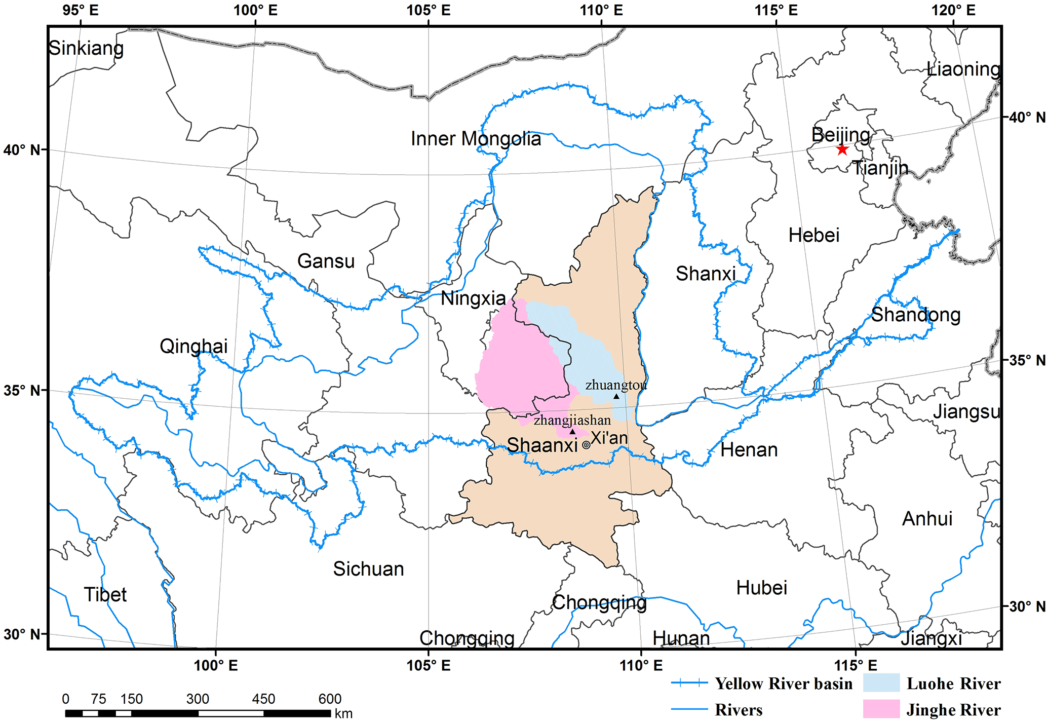
Figure 1Location of Shaanxi Province. Luohe and Jinghe watersheds were referred in the Table 5 and discussion part.
2.1 Sample and field survey
The design of the fourth census on soil erosion in China is based on a map with a Gauss–Krüger projection, where the whole of China was divided into 22 zones, with each zone occupying a width of 3∘ longitude (from the central meridian, 1.5∘ towards west and 1.5∘ towards east). Within each zone, beginning from the central meridian and the equator, we generated grids with a size of 40 km × 40 km (Fig. 2), which are the units at the first level (county level). The second level is township level, with a size of 10 km × 10 km. The third level is the control area, with a size of 5 km × 5 km. The fourth level is the 1 km × 1 km grid located in the middle of the control area. The 1 km × 1 km grid is the PSU in the plains area, whereas in the mountainous area, a small watershed with an area between 0.2 and 3 km2, which also intersects with the fourth-level 1 km × 1 km grid, was randomly picked as the PSU. The area for the mountainous PSU is restricted to be between 0.2–3 km2, which is large enough for the enumerator and not too large to be feasible to conduct field work. There is a PSU within every 25 km2, which suggests the designed sample density is about 4 %. In practice, due to the limitation of financial resources, the surveyed sample density is 1 % for most mountainous areas. The density for the plains area is reduced to 0.25 % due to the lower soil erosion risk (Li et al., 2012).
The field survey work for each PSU mainly included (1) recording the latitude and longitude information for the PSU using a GPS; (2) drawing boundaries of plots in a base map of the PSU; (3) collecting the information of land use and soil conservation measures for each plot; and (4) taking photos of the overview of PSUs, plots, and soil and water conservation measures for future validation. A plot was defined as the continuous area with the same land use, the same soil and water conservation measures, and the same canopy density and vegetation fraction in the PSU (difference 10 %, Fig. 3). For each plot, land use type, land use area, biological measures, engineering measures, and tillage measures were surveyed. In addition, the vegetation fraction was surveyed if the land use was a forest, shrubland, or grassland. Canopy density was also surveyed if the land use was a forest.
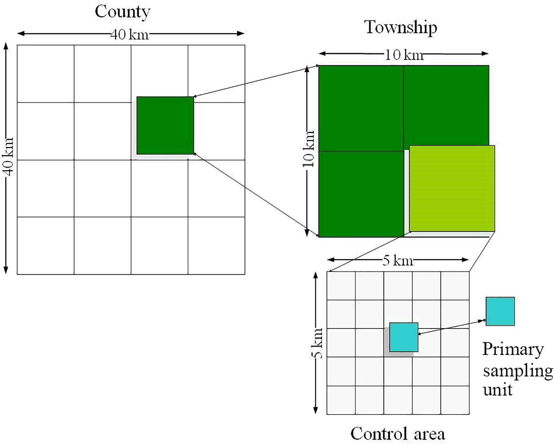
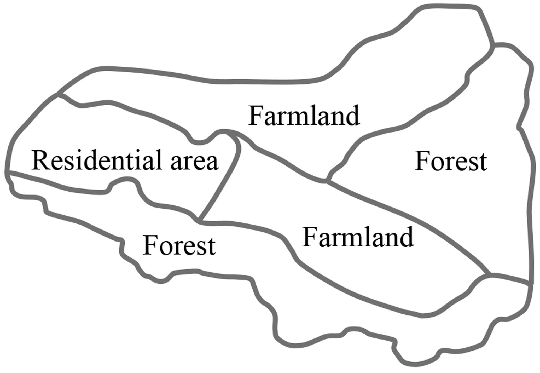
Figure 3An example of a Primary Sample Unit (PSU) with five plots and three categories of land use (farmland, forest, and residential area).

2.2 Database of PSUs in Shaanxi and its surrounding areas
A convex hull of the boundary of Shaanxi Province was generated, with a buffer area of 30 km outside of the convex hull (Fig. 4). The raster of the R factor, the K factor, and the 1 : 100 000 land use map with a resolution of 250 m × 250 m pixels for the entire area were collected. PSUs located inside the entire area were used, which included 1775 PSUs in the Shaanxi Province and 1341 PSUs from the provinces surrounding the Shaanxi Province, including Gansu (430), Henan (112), Shaanxi (345), Inner Mongolia (41), Hubei (151), Chongqing (55), Sichuan (156), and Ningxia (51). There were 3116 PSUs in total. We had the information of longitude and latitude, land use type, land use area, and factor values of R, K, L, S, B, E, and T for each plot of the PSU. The classification system of the land use for the entire area and that for the survey units were not synonymous with each other. Rather, they were grouped into 11 land use types, including (1) paddy, (2) dry land and irrigated land, (3) orchard and garden, (4) forest, (5) shrubland, (6) grassland, (7) waterbody, (8) construction land, (9) transportation land, (10) bare land, and (11) unused land such as sandy land, Gebi, and uncovered rock, so that they correspond to each other.
2.3 Soil loss estimation for the plot, land use, and PSU
Soil loss for a plot can be estimated using the CSLE as follows:
where Auk is the soil loss for the kth plot with the land use u (t ha−1 yr−1), Ruk is the rainfall erosivity (MJ mm ha−1 h−1 yr−1), Kuk is the soil erodibility (t ha h MJ−1 ha−1 mm−1), Luk is the slope length factor, Suk is the slope steepness factor, Buk is the biological practice factor, Euk is the engineering practice factor, and Tukis the tillage practice factor. The definitions of A, R, and K are similar to that of USLE. biological (B), engineering (E), and tillage (T) factors are defined as the ratios of soil loss from the actual plot with biological, engineering, or tillage practices to the unit plot. Biological practices are the measures to increase the vegetation coverage for reducing runoff and soil loss such as trees, shrubs, and grass plantation and natural rehabilitation of vegetation. Engineering practices refer to the changes of topography by engineering construction on both arable and nonarable land using non-normal farming equipment (such as an earth mover) for reducing runoff and soil loss, such as terraces and check dams. Tillage practices are the measures taken on the arable land during ploughing, harrowing, and cultivation processes using normal farming operations for reducing runoff and soil loss such as crop rotation and strip cropping (Liu et al., 2002).
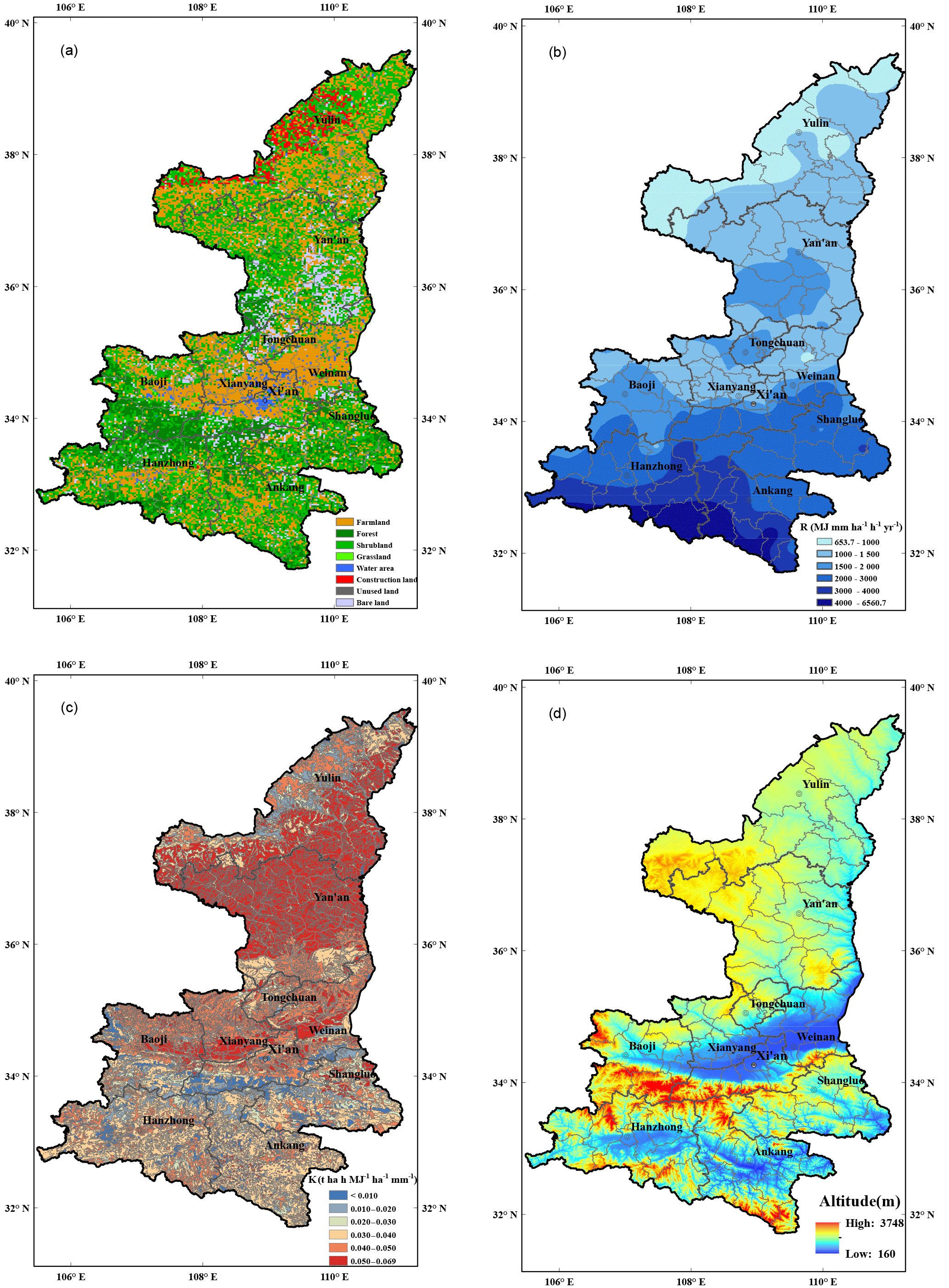
Figure 5Spatial distributions of land use (a), rainfall erosivity (b), soil erodibility (c) and topography (d) for Shaanxi Province.
Liu et al. (2013) introduced the data and methods for calculating each factor. Here we present a brief introduction. The land use map with a scale of 1 : 100 000 is from China's land use/cover datasets (CLUD), which were updated regularly at a 5-year interval from the late 1980s to the year 2010 with standard procedures based on Landsat TM/ETM images (Liu et al., 2014). The land use map used in this study was the 2010 version (Fig. 5a). A total of 2678 weather and hydrologic stations with erosive daily rainfall from 1981 to 2010 were collected and used to generate the R factor raster map over the whole of China (Xie et al., 2016). And for the K factor, soil maps with scales of 1 : 500 000 to 1 : 200 000 (for different provinces) from the Second National Soil Survey in the 1980s generated more than 0.18 million polygons of soil attributes over mainland China, which was the best available spatial resolution of soil information we could collect at present. The physicochemical data of 16 493 soil samples (belonging to 7764 soil series, 3366 soil families, 1597 soil subgroups, and 670 soil groups according to the Chinese Soil Taxonomy) from the maps and the latest soil physicochemical data of 1065 samples through field sampling, data sharing, and consulting literature were collected to generate the K factor for the entire country (Liang et al., 2013; Liu et al., 2013). We assumed the result of the soil survey could be used to estimate the K factor in our soil erosion survey. The R factor raster map for the study area was extracted from the map of the country as well as the K factor raster map (Fig. 5b and c). Topography contour maps with a scale of 1 : 10 000 for PSUs were collected to derive the slope lengths and slope degrees and to calculate the slope length factors and slope steepness factors (Fu et al., 2013). Topography contour maps with a scale of 1 : 10 000 for the entire region were not available at present. Figure 5d was based on the SRTM 90 m DEM dataset and it was used to demonstrate the variation in the topography. The land use map was used to determine the boundaries of forest, shrubland, and grassland. For these three land use types, MODIS NDVI and HJ-1 NDVI were combined to derive vegetation coverage. For the shrubland and grassland, an assignment table was used to assign a value of the half-month B factor based on their vegetation coverage; for the forestland, the vegetation coverage derived from the aforementioned remote sensing data was used as the canopy density, which was combined with the vegetation fraction under the trees collected during the field survey to estimate the half-month B factor. The B factor for the whole year was weight-averaged by the weight of the rainfall erosivity ratio for this half-month. Both the C factor in Panagos et al. (2015a) and the B factor in this study for forest, shrubland, and grassland were estimated based on the vegetation density derived from satellite images. The difference is that the C factor in Panagos et al. (2015a) for arable land and nonarable land was estimated separately based on different methodologies, whereas in this study, the B factor was used to reflect biological practices on the forest, shrubland, or grassland for reducing runoff and soil loss and the T factor was used to reflect tillage practices on the farmland for reducing runoff and soil loss. For farmland, the biological factor equals 1 and for the other land uses, the tillage factor equals 1. The engineering practice factor and tillage practice factor were values assigned based on the field survey and assignment tables for different engineering and tillage measures, which were obtained from published sources (Guo et al., 2015a).
In a PSU, there may be several plots within the same land use. Soil loss for the same land use was weight-averaged by the area of the plots with the same land use:
where Aui is the average soil loss for the land use u in the sample unit i (t ha−1 yr−1); Auik is the soil loss for the plot k with the land use u (t ha−1 yr−1); Suik is the area for the plot k with the land use u (ha). q is the number of plots with the land use u in the unit i.
2.4 Seven spatial models based on the BPST method
2.4.1 Seven spatial models
-
Model I estimates A with the land use as the auxiliary information. For the waterbody, transportation land and unused area, the estimation of soil loss for the uth land use and jth pixel was set to be zero. For the rest of the land use types, Aui for each land use was interpolated separately first and soil loss values for the entire domain are the combination of estimation for all land uses.
-
Model II estimates A with R and land use as the auxiliary information. For each sampling unit i in land use u, we define
where Rui is the rainfall erosivity value. For land use u, we smooth Qui over the entire domain using the longitude and latitude information and obtain the estimator of Quj for every pixel j. Then, for the jth pixel in land use u, we estimate the soil loss Auj by
-
Model III estimates A with K and land use as the auxiliary information. This model is similar to Model II, except that we use Kui instead of Rui in Eq. (3) and Kuj instead of Ruj in Eq. (4).
-
Model IV estimates A with L and land use as the auxiliary information. This model is similar to Model II, except that we use Lui instead of Rui in Eq. (3) and Luj instead of Ruj in Eq. (4).
-
Model V estimates A with S and land use as the auxiliary information. This model is similar to Model II, except that we use Sui instead of Rui in Eq. (3) and Suj instead of Ruj in Eq. (4).
-
Model VI estimates A with R, K, and land use as the auxiliary information. This model is similar to Model II, except that we use RuiKui instead of Rui in Eq. (3) and RujKuj instead of Ruj in Eq. (4).
-
Model VII estimates A with R, K, L, S, and land use as the auxiliary information. This model is similar to Model II, except that we use RuiKuiLuiSui instead of Rui in Eq. (3) and RujKujLujSuj instead of Ruj in Eq. (4).
2.4.2 Bivariate penalized spline over triangulation method
In spatial data analysis, there are mainly two approaches to make the prediction of a target variable. One approach (e.g., kriging) treats the value of a target variable at each location as a random variable and uses the covariance function between these random variables or a variogram to represent the correlation; another approach (e.g., spline or wavelet smoothing) uses a deterministic smooth surface function to describe the variations and connections among values at different locations. In this study, the bivariate penalized spline over triangulation (BPST) method, which belongs to the second approach, was used to explore the relationship between location information in a two-dimensional (2-D) domain and the response variable. The BPST method we consider in this work has several advantages. First, it provides good approximations of smooth functions over complicated domains. Second, the computational costs for spline evaluation and parameter estimation are manageable. Third, the BPST does not require the data to be evenly distributed or on a regular-spaced grid.
To be more specific, let (xi, yi) ∈ Ω be the latitude and longitude of unit i for i = 1, 2, …, n. Suppose we observe zi at locations (xi, yi) and {(xi, yi, satisfies
where εi is a random variable with mean zero, and f(xi, yi) is some smooth but unknown bivariate function. To estimate f, we adopt the bivariate penalized splines over triangulations to handle irregular domains. In the following we discuss how to construct basis functions using bivariate splines on a triangulation of the domain Ω. Details of various facts about bivariate splines stated in this section can be found in Lai and Schumaker (2007). See also Guillas and Lai (2010) and Lai and Wang (2013) for statistical applications of bivariate splines on triangulations.
A triangulation of Ω is a collection of triangles Δ = τ1τ2, …, τN whose union covers Ω. In addition, if a pair of triangles in Δ intersects, then their intersection is either a common vertex or a common edge. For a given triangulation Δ, we can construct Bernstein basis polynomials of degree p separately on each triangle, and the collection of all such polynomials form a basis. In the following, let be a spline space of degree p and smoothness r over triangulation Δ. Bivariate B splines on the triangulation are piecewise polynomials of degree p (polynomials on each triangle) that are smoothly connected across common edges, in which the connection of polynomials on two adjacent triangles is considered smooth if directional derivatives up to the rth degree are continuous across the common edge.
To estimate f, we minimize the following penalized least-squares problem:
where λ is the roughness penalty parameter, and PEN(f) is the penalty given below:
For Models I–VII defined in Sect. 2.4.1, we consider the above minimization to fit the model, and we obtain the smoothed surface using the Q data and their corresponding location information.
2.5 Assessment methods
The mean squared prediction error (MSE) and the Nash–Sutcliffe model efficiency coefficient (ME) are used to assess the performance of models. We estimate the out-of-sample prediction errors of each method using the ten-fold cross-validation. We randomly split all the observations over the entire domain (with the buffer zone) into 10 roughly equal-sized parts. For each t = 1, 2, …, 10, we leave out part t, fit the model using the other nine parts (combined) inside the boundary with the buffer zone, and then obtain predictions for the left-out tth part inside the boundary of Shaanxi Province. The overall mean squared prediction error (MSEoverall) is calculated by the average of the sum of the product of individual MSEu and the corresponding sample size. We first calculated the MSE of land each use u, u = 1, 2, …, 11:
where SSEt is the sum of squared prediction errors for the tth part. Then, the overall MSE can be calculated using
where Cu is the sample size for the land use u.
Model efficiency coefficient MEu for the land use u is calculated as follows (Nash and Sutcliffe, 1970):
Apre,u(i) and Aobs,u(i) are the predicted and observed soil loss for the plot i for land use u. MEoverall stands for the overall model efficiency by pooling all samples for different land uses together. The ME compares the simulated and observed values relative to the line of perfect fit. The maximum possible value of ME is 1, and the higher the value, the better the model fit. An efficiency of ME < 0 indicates that the mean of the observed soil loss is a better predictor of the data than the model. The soil loss rate is divided into six soil erosion intensity levels, which were mild (less than 5 t ha−1 yr−1), slight (5–10 t ha−1 yr−1), moderate (10–20 t ha−1 yr−1), high (20–40 t ha−1 yr−1), severe (40–80 t ha−1 yr−1), and extreme (no less than 80 t ha−1 yr−1). Each pixel in the entire domain was classified into an intensity level according to Auj. The proportion of intensity levels, soil loss rates for different land uses, and the spatial distribution of soil erosion intensity levels were computed based on the soil erosion conditions of pixels located inside of the Shaanxi boundary.
2.6 Sensitivity analysis of topography factors derived from different resolutions of DEM on the regional soil loss estimation
Previous research has suggested topography factors should be derived from high-resolution topography information (such as 1 : 10 000 or topography contour maps with finer resolutions; Thomas et al., 2015). Topography factors based on topography maps with coarser resolutions (such as 1 : 50 000 or 30 m DEM) in the mountainous and hilly areas have large uncertainties (S. Y. Wang et al., 2016). Topography contour maps with a scale of 1 : 10 000 for the entire region were not available at present. To detect whether coarser resolution topography data available for the entire region, such as SRTM 30 and 90 m DEM, can be used as the covariate in the interpolation process, L and S factors were derived from 30 and 90 m DEM data, respectively (Fu et al., 2013). The L and S factors derived from the 1 : 10 000 topography map for PSUs were used for the cross-validation analysis of Model IV, V, and VII to determine the relative contribution of erosion factors as the covariates to the spatial estimation of soil loss. The L and S factors generated from 30 and 90 m DEM data, together with those generated from the 1 : 10 000 topography map, were used for the sensitivity analysis based on Model VII. MSEu and MSEall based on Eqs. (8) and (9) were used to assess the effect of DEM resolution, from which topography factors were derived, on the interpolation accuracy of soil loss.
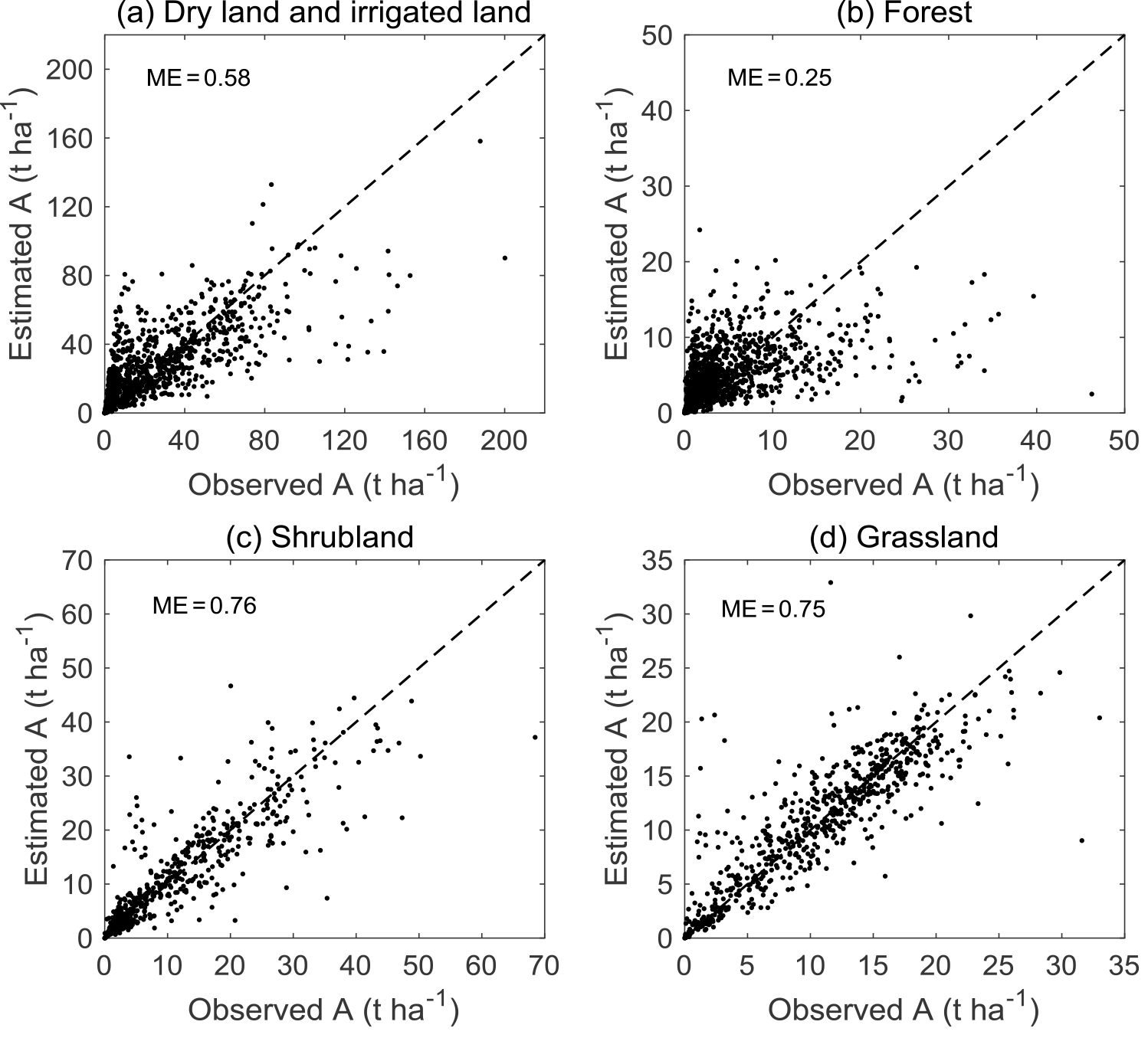
Figure 6Scatterplot of estimated and observed soil loss based on Model VII for (a) dry and irrigated land, (b) forest, (c) shrubland, and (d) grassland.
3.1 Comparison of MSEs and MEs for seven models and sensitivity of DEM resolution on the MSEs
Table 1 summarizes the MSEs of the soil loss estimation based on different methods. Model VII assisted by R, K, L, S, and land use generated the least overall MSE values and the best result, when L and S were derived based on the 1 : 10 000 topography map. MSE for Model VII was 55.8 % of that for Model I. The comparison of four models with the single erosion factor as the covariate (Model II–V) showed the S factor is the best covariate, with MSEoverall for Model V being 80.1 % of that for Model I, whereas R is the worst, with the MSEoverall for Model II being 99.3 % of that for Model I. For dry land and irrigated land and shrubland, Model II with the R factor and land use as the auxiliary information performed even worse than Model I assisted by the land use. K and L contributed the similar amount of information for the spatial model, decreasing the MSE about 10 % comparing with Model I. Model VI with R, K, and land use as the auxiliary information is superior to any model with land use and the single erosion factor as the covariates (Models I–V). When L and S factor were derived from 30 or 90 m DEM, the MSEs are much greater than Model I, which suggested the topography factors help the interpolation only if the resolution of DEM used to generate them is high enough, such as the 1 : 10 000 topography map. The use of factors derived from DEM with a resolution equal to or lower than 30 m seriously worsens the estimation.
Table 2 summarized the MEs for different land uses and overall data based on different models. All MEs were greater than 0, except four cases for the paddy land, which may be due to the limited sample size. Shrubland and grassland were the best estimated land use for Model I–VI. All seven models had an overall ME of no less than 0.55, with Model VII having the highest (0.75). The improvements of Model VII compared with the other six models were obvious for most land uses. Figure 6 showed the comparison of predicted and observed soil loss based on Model VII for four main land uses including dry land and irrigated land, forest, shrubland, and grassland, occupying 30.2, 15.9, 7.2, and 37.7 % of the total area for Shaanxi Province, respectively. It also showed the predictions of soil erosion in the shrubland and grassland were superior to those in the dry land and irrigated land and forest, the latter for which there was a degree of underestimation for larger soil loss values (Fig. 6).
Table 1Mean squared error of soil loss (A) using bivariate penalized spline over triangulation (BPST) for each type of land use1.
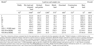
1 Since Fig. 6 showed no obvious systematic bias for four main land uses, we did not list the bias separately in this table. 2 Model I estimates A with the land use as the auxiliary information; Model II estimates with land use and the R factor as auxiliary information; Model III estimates with land use and the K factor as auxiliary information; Model IV estimates with land use and the L factor as auxiliary information; Model V estimates with land use and the S factor as auxiliary information; Model VI estimates with land use and R and K factors as auxiliary information; Model VII (1 : 10 000 map) estimates with land use and R, K, L, and S factors as auxiliary information and derives the L factor and S factor from 1 : 10 000 topography maps for the PSUs; Model VII (30 m DEM) estimates with land use and R, K, L, and S factors as auxiliary information and derives the L factor and S factor from 30 m SRTM DEM data for the PSUs; Model VII (90 m DEM) estimates with land use and R, K, L, and S factors as auxiliary information and derives the L and S factor from 90 m SRTM DEM data for the PSUs. 3 Sample size for each land use.
3.2 Soil erosion intensity levels and soil loss rates for different land uses
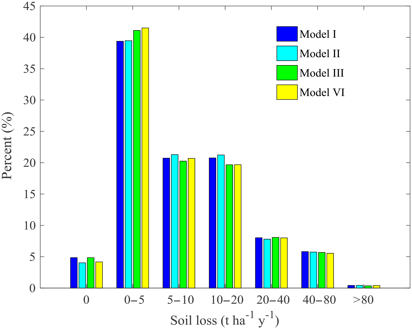
Models IV, V, and VII require the high resolution of topography maps to derive L and S factors, which we cannot afford in this study; therefore, four soil loss maps based on Models I, II, III, and VI were generated. The proportion pattern of soil erosion intensity levels for all land uses (Fig. 7) and that for different land use (Fig. 8) were very similar among the four models.

Figure 8Proportion of soil erosion intensity levels for different land use for four models including Model I–VI.
Table 2Model efficiency coefficient (ME) for seven models using bivariate penalized spline over triangulation (BPST) per land use.
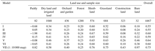
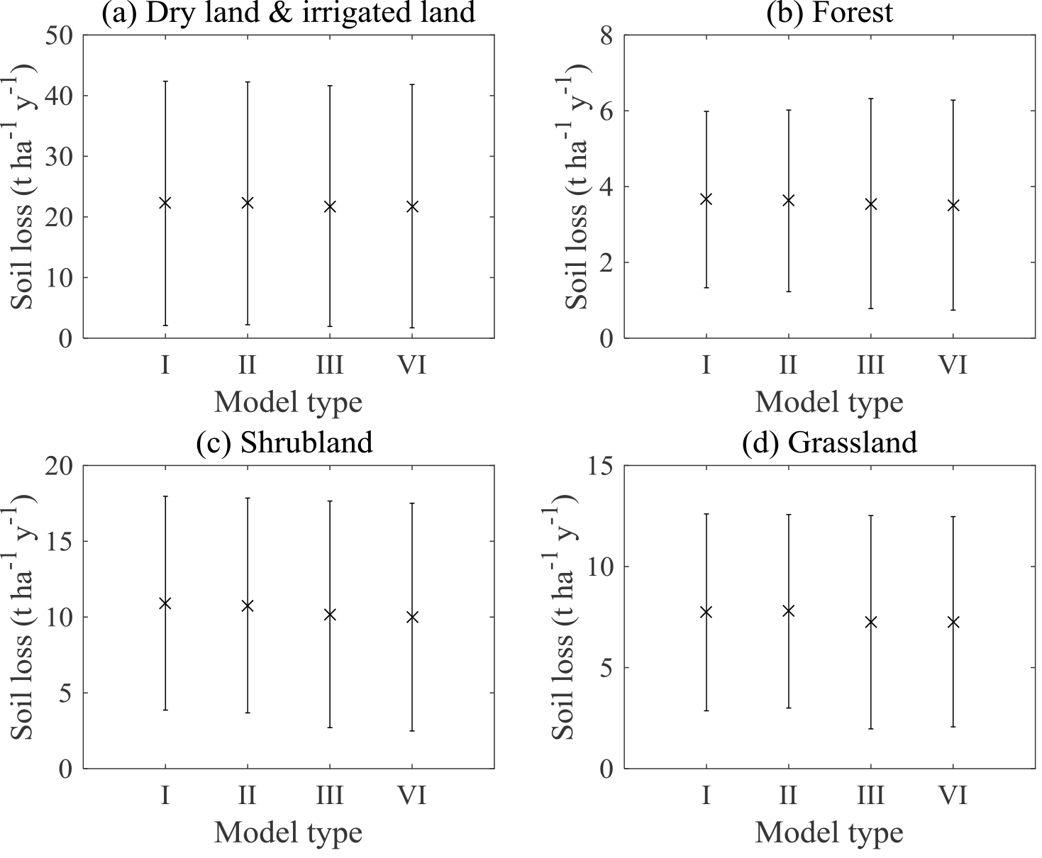
Figure 9Error bar plot of soil loss rates for four models for different land uses: (a) dry land and irrigated land, (b) forest, (c) shrubland, and (d) grassland. The star symbols stand for the mean values and the error bars stand for standard deviations.
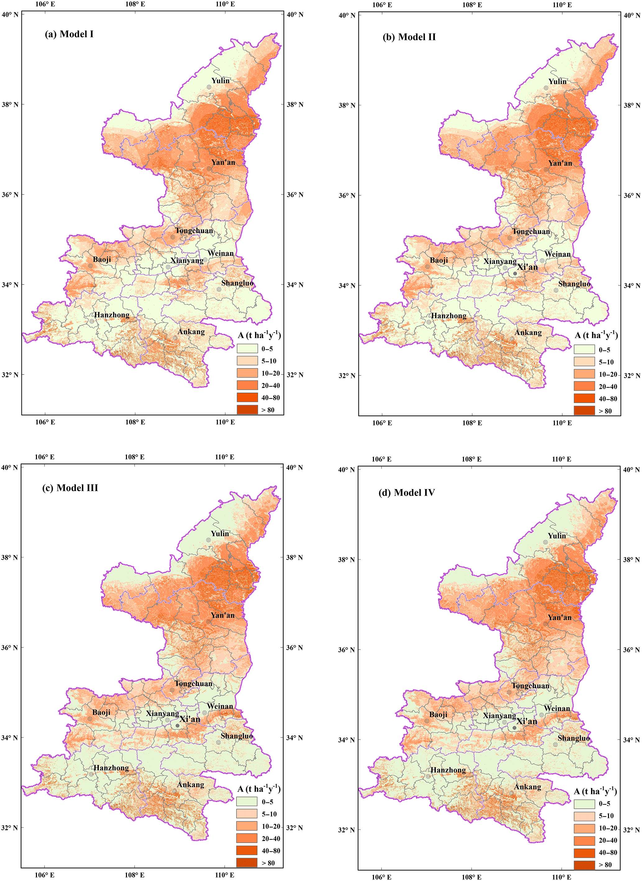
Figure 10Distribution of soil erosion intensity levels for four models: (a) Model I, (b) Model II, (c) Model III, and (d) Model VI.
The result of Model VI with the BPST method showed that the highest percentage is mild erosion (45.7 %), followed by the slight (20.7 %), moderate (19.7 %), and high erosion (8.0 %). The severe and extreme erosion were 5.5 and 0.4 %, respectively (Fig. 7). When it came to the land use (Fig. 8), the largest percentage for the dry land and irrigated land was high erosion, which occupied 23.2 % of the total dry land and irrigated land. The severe and extreme erosion for the dry land and irrigated land were 18.3 and 1.3 %, respectively. The largest percentage for the forestland and grassland was the mild erosion, being 75.1 and 41.7 %, respectively. The percentage of the mild, slight, and moderate erosion for the shrubland occupied about 30 %.
Figure 9 shows soil loss rates for the four main land uses generated from four models. Similar to the estimation of soil erosion intensity levels, there were slight differences among the four models. The soil loss rates for four main land uses (dry land and irrigated land, forest, shrubland, and grassland) by Model VI were reported in Table 3.
3.3 Spatial distribution of soil erosion intensity
All four models predicted generally similar spatial patterns of soil erosion intensity, with mild, moderate, and high erosion mainly occurring in the farmlands and grassland in the northern Loess Plateau region and severe and extreme soil erosion mainly occurring in the farmlands in the southern Qingba mountainous area (Fig. 10a–d). The estimation from Model VI showed that annual soil loss from Shaanxi Province was about 207.3 Mt, 49.2 % of which came from dry and irrigated lands and 35.2 % from grasslands (Table 4). The soil loss rate in Yan'an and Yulin in the northern part was 16.4 and 13.4 t ha−1 yr−1 and ranked the highest among 10 prefecture cities. More than half of the soil loss for the entire province was from these two districts (Table 4). Ankang and Hanzhong in the southern part also showed a severe soil loss rate and contributed nearly one-quarter of soil loss for the entire province. The soil loss rate in Tongchuan in the middle part was 10.2 t ha−1 yr−1, ranking the fourth most severe, whereas the total soil loss amount was 3.9 Mt, ranking last, due to its area being the smallest.
Table 3Soil loss rates (t ha−1yr−1) for farmland, forest, shrubland, and grassland by Model VI in this study and in the northwest region of China from Guo et al. (2015).
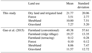
Table 4Annual soil loss amount, mean rate, and main sources by Model VI for 10 prefecture cities in Shaanxi Province.
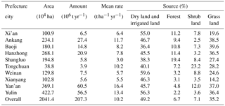
Table 5Soil erosion rate for the forest and sediment discharge for two watersheds.
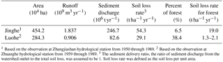
1 Based on the observation at Zhangjiashan hydrological station from 1950 through 1989. 2 Based on the observation at Zhuanghe hydrological station from 1959 through 1989. 3 The sediment delivery ratio, the ratio of sediment discharge from the watershed outlet to the total soil loss, was assumed to be 1. Soil loss rate was defined as the soil loss per unit area.
4.1 The uncertainty of the assessment
The uncertainty of the regional soil loss assessment method combining the survey sample and geostatistics mainly came from the estimation of erosion factors in the PSU, the density of survey sampling, and interpolation methods. Previous studies have shown that the resolution of topography data source largely affected the calculated slope steepness, length, and soil loss. Thomas et al. (2015) showed that the range of LS factor values derived from four sources of DEM (20 m DEM generated from 1 : 50 000 topographic maps, 30 m DEM from Advanced Spaceborne Thermal Emission and Reflection Radiometer – ASTER, 90 m DEM from SRTM, and 250 m DEM from global multi-resolution terrain elevation data – GMTED) were considerably different, which suggested the grid resolutions of factor layers are critical and determined by the data resolution used to derive the factor. S. Y. Wang et al. (2016) compared data sources including topographic maps at 1 : 2000, 1 : 10 000, and 1 : 50 000 scales and 30 m DEM from the ASTER V1 dataset and reported that slope steepness generated from the 30 m ASTER dataset was 64 % lower than the reference value generated from the 1 : 2000 topography map (2 m grid) for a mountainous watershed. The slope length was increased by 265 % and soil loss decreased by 47 % compared with the reference values. A study conducted by our research group indicated L and S factor and the soil loss prediction based on the DEM grid size less than or equal to 10 m were close to those of 2 m DEM (Fu et al., 2015); therefore, topography maps with a scale of 1 : 10 000 were collected in this study to derive the LS factor for the PSU. Note that R and K factors for PSUs were extracted from the map of the entire country, which may include some errors compared with those from at-site rainfall observations and soil field sampling for each PSU, which requires further research.
The density of sample units in our survey depends on the level of uncertainty and the budget of the survey. We tested sample density of 4 % in four experimental counties in different regions over China and found a density of 1 % was acceptable given the current financial condition. Since our data are a little sparse in some areas, we employed the roughness penalties to regularize the spline fit; see the energy functional defined in Eq. (7). When the sampling is sparse in a certain area, the direct BPST method may not be effective since the results may have high variability due to the small sample size. The BPST is more suitable for this type of data because the penalty regularizes the fit (Lai and Wang, 2013).
Cross-validation in Sect. 3.1 evaluated the uncertainty in the interpolation. The results consolidated the conclusion on the importance of topography factors and the DEM resolution used to calculate topography factors from previous research. It clarified that the S factor is the most important auxiliary factor in terms of the covariate in the interpolation of soil loss and K and L factors ranked the second most important, when topography factors were generated from a 1 : 10 000 map. Inclusion of topography factors from 30 m or coarser resolution of DEM data worsened the estimation.
4.2 Comparison with the other assessments
The Ministry of Water Resources of the People's Republic of China (MWR) has organized four nationwide soil erosion investigations. The first three (in the mid-1980s, 1999, and 2000) were mainly based on field surveys, visual interpretation by experts, and a factorial scoring method (X. Wang et al., 2016). The third investigation used 30 m resolution of Landsat TM images and 1 : 50 000 topography map. Six soil erosion intensities were classified, mainly based on the slope for the arable land and a combination of slope and vegetation coverage for the nonarable land. The limitations for the first three investigations include the limited resolution of satellite images and topography maps, limited soil erosion factors considered (rainfall erosivity factor, soil erodibility factor, and practice factor were not considered), incapability of generating the soil erosion rate, and incapability of assessing the benefit from the soil and water conservation practices. The spatial pattern of soil erosion in Shaanxi Province in this study is similar to the result of the third national investigation. Since the expert factorial scoring method did not generate the erosion rate for each land use, we compared the percentage of soil erosion area for 10 prefecture cities in Shaanxi Province with the third and the fourth investigations. Both investigations indicated that Yan'an and Yulin in the northern part, Tongchuan in the middle part, and Ankang in the southern part showed the most serious soil erosion. The difference is that Hanzhong was underestimated and Shangluo was overestimated in the third investigation, compared with the fourth investigation.
Guo et al. (2015a) analyzed 2823 plot-year runoff and soil loss data from runoff plots across five water erosion regions in China and compared the results with previous research around the world. The results convey that there were no significant differences for the soil loss rates of forest, shrubland, and grassland worldwide, whereas the soil loss rates of farmland with conventional tillage in northwest and southwest China were much higher than those in most other countries. Shaanxi Province is located in the northwest (NW) region. Soil loss rates for the farmland, forest, shrubland, and grassland based on the plot data for the NW region in Guo et al. (2015a) are extracted and presented in Table 3 for comparison. The soil loss rate for the farmland based on the plot data varied greatly with the management and conservation practices and the result in this study was within the range (Table 3). The soil loss rate for the shrubland is similar to that reported in Guo et al. (2015b). The soil loss rate for the forest in this study was 3.51 t ha−1 yr−1 with a standard deviation of 2.77 t ha−1 yr−1, which is much higher than 0.10 t ha−1 yr−1 reported in Guo et al. (2015a, Table 3). Our analysis proves that it came from the estimation of PSUs and was not introduced by the spatial interpolation process. Possible reasons include (1) the different definitions of forest and grassland, (2) concentrated storms with intense rainfall, (3) the unique topography in the Loess Plateau, and (4) the sparse vegetation cover due to intensive human activities (Zheng and Wang, 2014). The minimum canopy density (crown cover) threshold for the forest across the world varies from 10 to 30 % (Lambrechts et al., 2009) and a threshold of 10 % was used in this study, which suggests on average a lower vegetation coverage and a higher B factor. Annual average precipitation varies between 328 and 1280 mm in Shaanxi, with 64 % concentrated in June through September. Most rainfall comes from heavy storms of short duration, which suggests the erosivity density (rainfall erosivity per unit rainfall amount) is high. The field survey result on the PSUs in this study discovered that the slope degree is steeper and slope length is longer for the forest than the forest plots in Guo et al. (2015a). The forest plots in Guo et al. (2015a) were with an averaged slope degree of 25.9∘ and slope length of 21.1 m, whereas 74.0 % of forestland was with a slope degree greater than 25∘ and 97.2 % of them with a slope length longer than 20 m. The runoff and sediment discharge observation information for two watersheds (Fig. 1, Table 5) depicted that the soil loss rate for the forest in the study area has large variability ranging from 1.3 to 19.0 t ha−1 yr−1 (Wang and Fan, 2002). Our estimation is within the range. The soil loss rate for the grassland in this study was 7.27 t ha−1 yr−1, which was smaller than 11.57 t ha−1 yr−1 reported in Guo et al. (2015a). This may be due to the lower slope degree for the grassland in Shaanxi Province. The mean value of the slope degree for grassland plots was 30.7∘ in Guo et al. (2015a), whereas 68.6 % of the grasslands were with a slope degree smaller than 30∘ from the survey in this study.
Raster multiplication is a popular model-based approach due to its lower cost, simpler procedures, and easier explanation of resulting map. If the resolution of input data for the entire region is high enough to derive all the erosion factors, raster multiplication approach is the best choice. However, there are several concerns about raster multiplication approach for two reasons: (1) the information for the support practices factor (P) in the USLE was not easy to collect given the common image resolution and was not included in some assessments (Lu et al., 2001; Rao et al., 2015), in which the resulting maps do not reflect the condition of soil loss but the risk of soil loss. Without the information of the P factor, it is impossible to assess the benefit of the soil and water conservation practices (Liu et al., 2013). (2) The accuracy of the soil erosion estimation for each cell is of concern if the resolution of database used to derive the erosion factors is limited. For example, the LS factor in the new assessment of soil loss by water erosion in Europe (Panagos et al., 2015b) was calculated using the 25 m DEM, which may result in some errors for the mountainous and hilly areas due to the limited resolution of DEM data for each cell (S. Y. Wang et al., 2016). In this study, the information we can get at this stage for the entire region is land use, rainfall erosivity (R), and soil erodibility (K). The other factors were not available or did not have high enough resolution. It is not difficult to conduct raster layer multiplication technically; however, we think the multiplication of R and K factors (assuming L = 1, S = 1, B = 1, E = 1, T = 1) reflects the potential of soil erosion, which is different from the soil loss estimated in this study. Therefore, we did not compare our method with the raster layer multiplication method. Our recommended approach uses all the factor information that is available in the entire region (land use, rainfall, soils) and uses spatial interpolation to impute other factor information which is only available at the sampled PSU (slope degree, slope length, practice and management, aggregated as Q) to the entire region. The rationale behind this approach is to exploit the spatial dependence among these factors to come up with better regional estimates. Since the reality in many countries is that we cannot have all factors measured in all areas in the foreseeable future, or the resolution of data for deriving the factors is limited, we believe our approach provides a viable alternative which is of practical importance.
4.3 Practical implications
Remarkable spatial heterogeneity of soil erosion intensity was observed in the Shaanxi Province. The Loess Plateau region is one of the most severe soil erosion regions in the world due to seasonally concentrated and high intensity rainfall, high erodibility of loess soil, highly dissected landscape, and long-term intensive human activities (Zheng and Wang, 2014). Most of the sediment load in the Yellow River is originated and transported from the Loess Plateau. Recently, the sediment load of the Yellow River declined to about 0.3 billion tons per year from 1.6 billion tons per year in the 1970s, thanks to the soil and water conservation practices implemented in the Loess Plateau region (He, 2016). However, more efforts to control human accelerated soil erosion in the farmlands and grasslands are still needed. Soil erosion in the southern Qingba mountainous region is also very serious, which may be due to the intensive rainfall, farming in the steep slopes, and deforestation (Xi et al., 1997). According to the survey in Shaanxi Province, 11.1 % of the farmlands with a slope degree ranging 15–25∘ and 6.3 % of them with a slope degree greater than 25∘ did not have any conservation practices in place. Mountainous areas with a slope steeper than 25∘ need to be sealed off for afforestation (grass) without disturbance of humans and livestock. For those farmlands with a slope degree lower than 25∘, terracing and tillage practices are suggested, which can greatly reduce the soil loss rate (Guo et al., 2015a, Table 3). The survey result determined that 26.5 % of grasslands with a slope degree of 15–25∘ and 57.6 % with a slope degree steeper than 25∘ did not have any conservation practices in place. Enclosure and grazing prohibition are suggested on the grasslands with a steep slope and low vegetation coverage.
Note that the CSLE as well as other USLE-based models only simulate sheet and rill erosion, and erosion from gullies is not taken into consideration in this study. Erosion from gullies is also very serious in the Loess Plateau area, and there were more than 140 000 gullies longer than 500 m in Shaanxi Province (Liu, 2013).
This regional soil erosion assessment focused on the extent, intensity, and distribution of soil erosion on a regional scale and it provides valuable information for stakeholders to take proper conservation measures in erosion areas. Shaanxi Province is one of the most severe soil erosion regions in China. A field survey in 3116 PSUs in the Shaanxi Province and its surrounding areas was conducted, and the soil loss rates for each land use in the PSU were estimated from an empirical soil loss model (CSLE). Seven spatial interpolation models based on the BPST method were compared, which generated regional soil erosion assessment from the PSUs. The following is a summary of our conclusions.
-
The slope steepness (S) factor derived from a 1 : 10 000 topography map is the best single covariate. The MSE of the soil loss estimator using the model with the land use and S factor is 20 % less than those using the model assisted by the land use alone. Soil erodibility (K) and slope length (L) information each reduce about 10 % of the MSE. Contribution of rainfall erosivity (R) to the decrease of MSE is less than 1 %.
-
Model VII with the land use and R, K, L, S as the auxiliary information has a model efficiency of 0.75 and is superior to any model with land use and single or two erosion factors as the covariates (Model I–VI), which has a model efficiency varying from 0.55 to 0.64.
-
The LS factor derived from 30 or 90 m DEM was not useful when it was used as the covariate together with the land use, R, and K, with the MSEs increased by about 2 times compared with those for the model assisted by the land use alone.
-
Four models assisted by the land use (Model I), the land use and the R factor (Model II), the land use and the K factor (Model III), and the land use, the R factor, and the K factor (Model VI) provided similar estimates for proportions in each soil erosion intensity level, soil loss rates for different land uses, and spatial distribution of soil erosion intensity.
-
There is 54.3 % of total land in Shaanxi Province with annual soil loss rate no less than 5 t ha−1 yr−1, and total annual soil loss amount is about 207.3 Mt. Most soil loss originated from the farmlands and grasslands in Yan'an and Yulin districts in the northern Loess Plateau region and Ankang and Hanzhong districts in the southern Qingba mountainous region. Special attention should be given to the 0.11 million km2 of lands with soil loss rate equal to or greater than 5 t ha−1 yr−1, especially 0.03 million km2 of farmlands with severe and extreme erosion (greater than 20 t ha−1 yr−1).
-
A new model-based regional soil erosion assessment method was proposed, which is valuable when input data used to derive soil erosion factors are not available for the entire region or the resolution is not adequate. When the resolution of input datasets is not adequate to derive reliable erosion factor layers and the budget is limited, our suggestion is sampling a certain number of small watersheds as primary sampling units and putting the limited money into these sampling units to ensure the accuracy of soil erosion estimation in these units. Limited money could be used to collect high-resolution data such as satellite images and topography maps and conduct field research to collect information such as conservation practices for these small watersheds. Then we can use the best available raster layers for land use, R, and K factors for the entire region, construct spatial models to exploit the spatial dependence among the other factors, and combine them to generate better regional estimates. The information collected in the survey and the generated soil erosion degree map (such as Fig. 10d) can help policymakers to take suitable erosion control measures in the severely affected areas. Moreover, climate and management scenarios could be developed based on the database collected in the survey process to help policymakers in decision-making for managing soil erosion risks.
Data will be available on a dedicated database website after a contract is accepted on behalf of all institutions. Until then, the corresponding author can be contacted for any requests regarding data.
The authors declare that they have no conflict of interest.
This work was supported by the National Natural Science Foundation of China
(no. 41301281) and the China Scholarship Council.
Edited by: Axel Bronstert
Reviewed by: three anonymous referees
Bahrawi, J. A., Elhag, M., Aldhebiani, A. Y., Galal, H. K., Hegazy, A. K., and Alghailani, E.: Soil erosion estimation using remote sensing techniques in Wadi Yalamlam Basin, Saudi Arabia, Adv. Mater. Sci. Eng., 2016, 9585962, https://doi.org/10.1155/2016/9585962, 2016.
Blanco, H. and Lal, R.: Principles of Soil Conservation and Management, Springer, New York, 2010.
Bosco, C., de Rigo, D., Dewitte, O., Poesen, J., and Panagos, P.: Modelling soil erosion at European scale: towards harmonization and reproducibility, Nat. Hazards Earth Syst. Sci., 15, 225–245, https://doi.org/10.5194/nhess-15-225-2015, 2015.
Breidt, F. J. and Fuller, W. A.: Design of supplemented panel surveys with application to the National Resources Inventory, J. Agr. Biol. Environ. St., 4, 391–403, 1999.
Brejda, J. J., Mausbach, M. J., Goebel, J. J., Allan, D. L., Dao, T. H., Karlen, D. L., Moorman, T. B., and Smith J. L.: Estimating surface soil organic carbon content at a regional scale using the National Resource Inventory, Soil. Sci. Soc. Am. J., 65, 842–849, 2001.
Cerdan, O., Govers, G., Le Bissonais, Y., Van Oost, K., Poesen, J., Saby, N., Gobin, A., Vacca, A., Quinton, J., Auerswald, K., Klik, A., Kwaad, F. J. P. M., Raclot, D., Ionita, I., Rejman, J., Rousseva, S., Muxart, T., Roxo, M. J., and Dostal, T.: Rates and spatial variations of soil erosion in Europe: a study based on erosion plot data, Geomorphology, 122, 167–177, 2002.
El Haj El Tahir, M., Kääb, A., and Xu, C.-Y.: Identification and mapping of soil erosion areas in the Blue Nile, Eastern Sudan using multispectral ASTER and MODIS satellite data and the SRTM elevation model Hydrol. Earth Syst. Sci., 14, 1167–1178, https://doi.org/10.5194/hess-14-1167-2010, 2010.
Evans, R. and Boardman, J.: The new assessment of soil loss by water erosion in Europe, Panagos, P. et al., 2015 Environ. Sci. Policy, 54, 438–447 – A response, Environ. Sci. Policy, 58, 11–15, 2016.
Evans, R., Collins, A. L., Foster, I. D. L., Rickson, R. J., Anthony, S. G., Brewer, T., Deeks, L., Newell-Price, J. P., Truckell, I. G., and Zhang, Y.: Extent, frequency and rate of water erosion of arable land in Britain – benefits and challenges for modelling, Soil Use Manage., 32, 149–161, 2015.
Fiener, P. and Auerswald, K.: Comment on “The new assessment of soil loss by water erosion in Europe” by Panagos et al. (Environmental Science & Policy 54 (2015) 438–447), Environ. Sci. Policy, 57, 140–142, 2016.
Foster, G. R.: User's Reference Guide: Revised Universal Soil Loss Equation (RUSLE2), US Department of Agriculture, Agricultural Research Service, Washington, D.C., 2004.
Fu, S. H., Cao, L. X., Liu, B. Y., Wu, Z. P., and Savabi, M. R.: Effects of DEM grid size on predicting soil loss from small watersheds in China, Environ. Earth Sci., 73, 2141–2151, 2015.
Fu, S. H., Wu, Z. P., Liu, B. Y., and Cao, L. X.: Comparison of the effects of the different methods for computing the slope length factor at a watershed scale, Int. Soil Water Conserv. Res., 1, 64–71, 2013.
Ganasri, B. P. and Ramesh, H.: Assessment of soil erosion by RUSLE model using remote sensing and GIS – A case study of Nethravathi Basin, Geosci. Front., 7, 953–961, 2015.
Gobin, A., Jones, R., Kirkby, M. J., Campling, P., Govers, G., Kosmas, C., and Gentile, A. R.: Indicators for pan-European assessment and monitoring of soil erosion by water, Environ. Sci. Policy, 7, 25–38, 2004.
Goebel, J. J.: The National Resources Inventory and its role in U.S. agriculture, Agricultural Statistics 2000, International Statistical Institute, Voorburg, 1998.
Grimm, M., Jones, R., and Montanarella, L.: Soil erosion risk in Europe, European Commission, EUR 19939 EN, Joint Research Centre, Ispra, 2002.
Grimm, M., Jones, R., Rusco, E. and Montanarella, L.: Soil Erosion Risk in Italy: a revised USLE approach, EUR 20677 EN, European Commission, Luxembourg, 2003.
Guillas, S. and Lai, M. J.: Bivariate splines for spatial functional regression models, J. Nonparametr. Statist., 22, 477–497, 2010.
Guo, Q. K., Hao, Y. F., and Liu, B. Y.: Rates of soil erosion in China: A study based on runoff plot data, Catena, 24, 68–76, 2015a.
Guo, Q. K., Liu, B. Y., Xie, Y., Liu, Y. N., and Yin, S. Q.: Estimation of USLE crop and management factor values for crop rotation systems in China, J. Integr. Agr., 14, 1877–1888, 2015b.
Guo, S. Y. and Li, Z. G.: Development and achievements of soil and water conservation monitoring in China, Sci. Soil Water Conserv., 7, 19–24, 2009.
He, C. S.: Quantifying drivers of the sediment load reduction in the Yellow River Basin, National Sci. Rev., 3, 155–156, https://doi.org/10.1093/nsr/nww014, 2016.
Hernandez, M., Nearing, M. A., Stone, J. J., Pierson, E. B., Wei, H., Spaeth, K. E., Heilman, P., Weltz, M. A., and Goodrich, D. C.: Application of a rangeland soil erosion model using National Resources Inventory data in southeastern Arizona, J. Soil Water Conserv., 68, 512–525, 2013.
Herrick, J. E., Lessard, V. C., Spaeth, K. E., Shaver, P. L., Dayton, R. S., Pyke, D. A., Jolley, L., and Goebel, J. J.: National ecosystem assessments supported by scientific and local knowledge, Front. Ecol. Environ., 8, 403–408, 2010.
Kirkby, M. J., Irvine, B. J., Jones, R. J. A., Govers, G., Boer, M., Cerdan, O., Daroussin, J., Gobin, A., Grimm, M., Le Bissonnais, Y., Kosmas, C., Mantel, S., Puigdefabregas, J., and van Lynden, G.: The PESERA coarse scale erosion model for Europe. I. – Model rationale and implementation, Eur. J. Soil Sci., 59, 1293–1306, 2008.
Lai, M. J. and Schumaker, L. L.: Spline functions on triangulations, Cambridge University Press, Cambridge, 2007.
Lai, M. J. and Wang, L.: Bivariate penalized splines for regression, Statist. Sin., 23, 1399–1417, 2013.
Lambrechts, C., Wilkie, M. L., Rucevska, I., and Sen, M. (Eds.): Vital Forest Graphics, United Nations Environment Programme (UNEP), United Nations Food and Agriculture Organisation (FAO), United Nations Forum on Forests (UNFF), UNEP/GRID-Arendal, Arendal, Norway, 2009.
Le Bissonnais, Y., Montier, C., Jamagne, M., Daroussin, J., and King, D.: Mapping erosion risk for cultivated soil in France, Catena, 46, 207–220, 2001.
Le Roux, J. J., Newby, T. S., and Sumner, P. D.: Monitoring soil erosion in South Africa at a regional scale: review and recommendations, S. Afr. J. Sci., 207, 329–335, 2007.
Li, Z. G., Fu, S. H., and Liu, B. Y.: Sampling program of water erosion inventory in the first national water resource survey, Sci. Soil Water Conserv., 10, 77–81, 2012.
Liang, Y., Liu, X. C., Cao, L. X., Zheng, F. L., Zhang, P. C., Shi, M. C., Cao, Q. Y., and Yuan, J. Q.: K value calculation of soil erodibility of China water erosion areas and its Macro-distribution, Soil Water Cons. China, 10, 35–40, 2013.
Liu, B. Y., Zhang, K. L., and Xie, Y.: An empirical soil loss equation, in Proceedings – Process of soil erosion and its environment effect (Vol. II), 12th international soil conservation organization conference, Tsinghua University Press, Beijing, 21–25, 2002.
Liu, B. Y., Guo, S. Y., Li, Z. G., Xie, Y., Zhang, K. L., and Liu, X. C.: Sample survey on water erosion in China, Soil Water Conserv. China, 10, 26–34, 2013.
Liu, J. Y., Kuang, W. H., Zhang, Z. X., Xu, X. L., Qin, Y. W., Ning, J., Zhou, W. C., Zhang, S. W., Li, R. D., Yan, C. Z., Wu, S. X., Shi, X. Z., Jiang, N., Yu, D. S., Pan, X. Z., and Chi, W. F.: Spatiotemporal characteristics, patterns and causes of land use changes in China since the late 1980s, Acta Geogr. Sin., 69, 3–14, 2014.
Liu, Z.: The national census for soil erosion and dynamic analysis in China, Int. Soil Water Conserv. Res., 1, 12–18, 2013.
Lu, H., Gallant, J., Prosser, I. P., Moran, C., and Priestley, G.: Prediction of sheet and rill erosion over the Australian continent, incorporating monthly soil loss distribution, CSIRO Land and Water Technical Report, CSIRO, Canberra, 2001.
Morgan, R. P. C.: Soil Erosion and Conservation, 2nd Edn., Longman, Essex, 1995.
Mutekanga, F. P., Visser, S. M., Stroosnijder, L.: A tool for rapid assessment of erosion risk to support decision-making and policy development at the Ngenge watershed in Uganda, Geoderma, 160, 165–174, 2010.
Nash, J. E. and Sutcliffe, J. V.: River flow forecasting through conceptual models, Part 1 – a discussion of principles, J. Hydrol., 10, 282–290, 1970.
Nusser, S. M. and Goebel, J. J.: The National Resources Inventory: A long-term multi-resource monitoring programme, Environ. Ecol. Stat., 4, 181–204, 1997.
Panagos, P., Borrelli, P., Meusburger, K., Alewell, C., Lugato, E., and Montanarella, L.: Estimating the soil erosion cover-management factor at the European scale, Land Use Policy, 48, 38–50, 2015a.
Panagos, P., Borrelli, P., Poesen, J., Ballabio, C., Lugato, E., Meusburger, K., Montanarella, L., and Alewell, C.: The new assessment of soil loss by water erosion in Europe, Environ. Sci. Policy, 54, 438–447, 2015b.
Panagos, P., Borrelli, P., Poesen, J., Meusburger, K., Ballabio, C., Lugato, E., Montanarella, L., and Alewell, C.: Reply to “The new assessment of soil loss by water erosion in Europe. Panagos P. et al., 2015 Environ. Sci. Policy 54, 438–447 – A response” by Evans and Boardman [Environ. Sci. Policy 58, 11–15], Environ. Sci. Policy, 59, 53–57, 2016a.
Panagos, P., Borrelli, P., Poesen, J., Meusburger, K., Ballabio, C., Lugato, E., Montanarella, L., and Alewell, C.: Reply to the comment on “The new assessment of soil loss by water erosion in Europe” by Fiener & Auerswald, Environ. Sci. Policy, 57, 143–150, 2016b.
Rao, E. M., Xiao, Y., Ouyang, Z. Y., and Yu, X. X.: National assessment of soil erosion and its spatial patterns in China, Ecosyst. Health Sustain., 1, 1–10, https://doi.org/10.1890/EHS14-0011.1, 2015.
Renard, K. G., Foster, G. R.,Weesies, G. A., McCool, D. K., and Yoder, D. C.: Predicting soil erosion by water, in: Agriculture Handbook 703, US Department of Agriculture, Agricultural Research Service, Washington, D.C., 1997.
Renschler, C. S. and Harbor, J.: Soil erosion assessment tools from point to regional scales – the role of geomorphologists in land management research and implementation, Geomorphology, 47, 189–209, 2002.
Singh, G., Babu, R., Narain, P., Bhushan, L. S., and Abrol, I. P.: Soil erosion rates in India, J. Soil Water Conserv., 47, 97–99, 1992.
Thomas, J., Prasannakumar, V., and Vineetha, P.: Suitability of spaceborne digital elevation models of different scales in topographic analysis: an example from Kerala, India, Environ. Earth Sci., 73, 1245–1263, 2015.
USDA: Summary report: 2012 National Resources Inventory, National Resources Conservation Service, Washington, D.C., and Center for Survey Statistics and Methodology, Iowa State University, Ames, Iowa, 2015.
Van der Knijff, J. M., Jones, R. J. A., and Montanarella, L.: Soil erosion risk assessment in Europe, EUR 19044 EN, European Commission, Luxembourg, 2000.
Vrieling, A.: Satellite remote sensing for water erosion assessment: A review, Catena, 65, 2–18, 2006.
Wang, G. and Fan, Z.: Study of Changes in Runoff and Sediment Load in the Yellow River (II), Yellow River Water Conservancy Press, Zhengzhou, China, 2002.
Wang, S. Y., Zhu, X. L., Zhang, W. B., Yu, B., Fu, S. H., and Liu, L.: Effect of different topographic data sources on soil loss estimation for a mountainous watershed in Northern China, Environ. Earth Sci., 75, 1382, https://doi.org/10.1007/s12665-016-6130-3, 2016.
Wang, X., Zhao, X. L., Zhang, Z. X., Li, L., Zuo, L. J., Wen, Q. K., Liu, F., Xu, J. Y., Hu, S. G., and Liu, B.: Assessment of soil erosion change and its relationships with land use/cover change in China from the end of the 1980s to 2010, Catena, 137, 256–268, 2016.
Wischmeier, W. H. and Smith, D. D.: Predicting rainfall-erosion losses from cropland east of the Rocky Mountains, in: Agriculture Handbook 282, US Department of Agriculture, Agricultural Research Service, Washington, D.C., 1965.
Wischmeier, W. H. and Smith, D. D.: Predicting Rainfall Erosion Losses: A Guide to Conservation Planning, in: Agriculture Handbook 537, US Department of Agriculture, Agricultural Research Service, Washington, D.C., 1978.
Xi, Z. D., Sun, H., and Li, X. L.: Characteristics of soil erosion and its space-time distributive pattern in southern mountains of Shaanxi province, Bull. Soil Water Conserv., 17, 1–6, 1997.
Xie, Y., Yin, S. Q., Liu, B. Y., Nearing, M., and Zhao, Y.: Models for estimating daily rainfall erosivity in China, J. Hydrol., 535, 547–558, 2016.
Zheng, F. L. and Wang, B.: Soil Erosion in the Loess Plateau Region of China, in: Restoration and Development of the Degraded Loess Plateau, China, Ecological Research Monographs, edited by: Tsunekawa, A., Liu, G., Yamanaka, N., and Du, S., Springer, Japan, https://doi.org/10.1007/978-4-431-54481-4_6, 2014.