Continental water storage trends and budgets from the GRACE/GRACE-FO Global Gravity-based Groundwater Product (G3P)

The Global Gravity-based Groundwater Product (G3P) provides global groundwater storage (GWS) variations derived from GRACE/GRACE-FO terrestrial water storage (TWS) change by subtracting root-zone soil moisture, glacier mass change, surface water storage, and snow water equivalent. G3P thus provides the first globally consistent, publicly available groundwater dataset from satellite gravimetry for continental-scale water resources assessment. Here, we use G3P to assess global GWS trends over the extended GRACE/GRACE-FO record, jointly with TWS and the subtracted storage components.

A central challenge is that apparent long-term trends in GRACE/GRACE-FO water storage records can reflect persistent storage change, natural climate variability, hydrological memory, and observational errors, complicating trend detection and continental-scale storage-change budgets. We address this using a calibrated trend-analysis framework that jointly accounts for trend, seasonal, and stochastic variations in each grid-cell time series. Statistically significant trends are then aggregated to quantify volumetric GWS and TWS gains, losses, and net changes at continental and global scales.

Applying this framework to 21.5 years of data (April 2002–September 2023), we find that groundwater depletion is a major contributor to freshwater decline at continental scales, most prominently in Asia (−55 km³ yr⁻¹), while cryospheric mass loss dominates the strongest TWS declines in high-latitude and glacierized regions. Pronounced regional contrasts include increasing groundwater storage across large parts of Africa (+37 km³ yr⁻¹), negative trends in drought-affected regions, and widespread negative or near-threshold GWS tendencies across the Northern Hemisphere. Globally, significance-filtered net GWS and TWS changes are approximately −27 and −183 km³ yr⁻¹, respectively. The corresponding gross negative GWS change of approximately 103 km³ yr⁻¹ is of the same order as model-based estimates of global groundwater depletion. Sensitivity tests indicate robust results: at 95 %, detected area increases by 30 % for TWS and 36 % for GWS, while net-loss magnitudes rise by only 9 % and 18 %. Across much of the seasonal-to-interannual spectral range, GWS is the dominant individual storage-component signal within TWS, which highlights the importance of groundwater for continental freshwater availability.

1 Introduction

1.1 Water storage: an Essential Climate Variable observed by satellite gravimetry

Quantifying trends in terrestrial water storage (TWS) is central for assessing changes in global freshwater availability and its coupling to the climate system (Rodell et al., 2018; Pokhrel et al., 2021). TWS integrates changes in groundwater storage (GWS), soil moisture, surface water, snow water equivalent, and glaciers. To reflect their importance, TWS and GWS have been endorsed as Essential Climate Variables by the Global Climate Observing System (GCOS) (World Meteorological Organization, 2022).

Since 2002, the GRACE (2002–2017) and GRACE Follow-On (since 2018) missions provide global observations of time-variable mass change (Tapley et al., 2004; Landerer et al., 2020), yielding an almost continuous over-two-decade record that substantially improves trend detectability compared to earlier GRACE-only studies. Within the Global Gravity-based Groundwater Product (G3P), consistent global GWS estimates (v1.12) are derived from GRACE/GRACE-FO TWS by subtracting contributions of other storage compartments (Güntner et al., 2026). GRACE/GRACE-FO observations capture the combined effects of climate variability, cryospheric mass loss, and anthropogenic water use, including groundwater extraction for irrigation (e.g., Li and Rodell, 2024). For global trend assessment, GRACE/GRACE-FO observations are particularly valuable because hydrological and land-surface models can exhibit divergent trend signs and magnitudes, which complicates trend inference (e.g., Scanlon et al., 2018 or Albergel et al., 2012).

1.2 Observed global and continental-scale patterns in TWS and GWS

GRACE-based assessments indicate spatially heterogeneous TWS trends. For 2002–2016, Rodell et al. (2018) quantified 34 major regional TWS trends and attributed them to natural interannual variability, unsustainable groundwater consumption, climate change, or combinations thereof. Their analysis highlighted strong cryospheric losses in North America as well as major drying regions in Asia and other continents. In contrast, for Africa positive TWS tendencies in parts of the Sahel and East Africa are reported, attributed to precipitation variability and enhanced groundwater recharge, the so-called Sahelian Paradox (Werth et al., 2017; Springer et al., 2023). South America shows moderate losses dominated by Patagonian glacier retreat, while strong variability driven by El Niño Southern Oscillation (ENSO) is a complicating factor for detection in the Amazon Basin (Satizábal-Alarcón et al., 2024). Regarding recent synthesis efforts, Chandanpurkar et al. (2025) report a global land TWS loss equivalent to 324 ± 55 km³ yr⁻¹ (excluding Greenland and Antarctica), using a different spatial and methodological framework; this is one of the largest published global land TWS loss estimates to date.

GWS represents a substantial and regionally heterogeneous component of TWS change. Global anthropogenic groundwater depletion has been estimated at approximately 100–150 km³ yr⁻¹ during the early 21st century, with some model-based estimates reaching up to about 200 km³ yr⁻¹ (Döll et al., 2014; de Graaf et al., 2017; Bierkens and Wada, 2019). However, regional groundwater gains partly compensate for these losses, which results in substantially smaller net global groundwater storage declines. For 2002–2014, Wada et al. (2017) partition global land water storage change by process. Summing the loss terms in their budget – groundwater depletion, endorheic and wetland losses, and deforestation – groundwater accounts for about half of the total, which makes it the largest single loss term. In contrast, for the GRACE/GRACE-FO era, Chandanpurkar et al. (2025) report that groundwater depletion accounts for about 68 % of TWS loss over non-glaciated continental regions. Large-scale analyses based on groundwater well observations confirm widespread groundwater decline, along with localized recovery resulting from policy interventions (Jasechko et al., 2024). Major depletion hotspots are the Indo-Gangetic Plain, North China Plain, and the Middle East (Rodell et al., 2009; Feng et al., 2013; Joodaki et al., 2014), as well as the High Plains Aquifer and California's Central Valley in North America (Scanlon et al., 2012; Famiglietti et al., 2011). In Africa, positive GWS anomalies in parts of the Niger Basin and the East African Rift are in contrast to depletion in North African fossil aquifer systems, notably the North Western Sahara Aquifer System (NWSAS) and the Nubian Sandstone Aquifer System (NSAS) (Werth et al., 2017; Springer et al., 2023).

1.3 Physical drivers, attribution, and interpretation limits

Attribution of TWS and GWS trends to climate-related and anthropogenic drivers is important, yet challenging. Cryospheric mass loss is a dominant component of global land-mass decline, with Greenland and Antarctica losing approximately 169 ± 9 and 92 ± 18 Gt yr⁻¹, respectively, over 1992–2020, while glaciers outside the Greenland and Antarctic ice sheets lost approximately 199 ± 32 Gt yr⁻¹ over 2002–2016 (Wouters et al., 2019; Otosaka et al., 2023). Outside glaciated regions, groundwater abstraction for irrigation is a major driver of persistent groundwater-storage decline in intensively managed aquifers. In many systems under stress, groundwater extraction exceeds renewable groundwater availability, which results in continued depletion of groundwater storage (Wada et al., 2012; Richey et al., 2015).

Climate variability is linked to large-scale modes such as ENSO, the North Atlantic Oscillation, and the Indian Ocean Dipole and is known to modulate precipitation, soil moisture, surface water, and groundwater recharge on interannual to decadal time scales (Anyah et al., 2018; Boergens et al., 2024). Assessments indicate that, when integrating across storage compartments, climate forcing may exceed anthropogenic contributions to decadal land water storage change, although this is reported to strongly depend on the region (Scanlon et al., 2018). TWS trends also propagate into sea-level budgets and Earth-system mass closure, and provide constraints on coupled hydrosphere–cryosphere processes (Riva et al., 2010; Frederikse et al., 2020). However, uncertainties across storage components remain substantial and yet unsolved (e.g., Dorigo et al., 2021).

Hydrological memory is a limiting factor for trend interpretation: groundwater and glaciers contain multi-year climate signals, whereas soil moisture and surface water respond more rapidly. These memory effects, often underrepresented in models, can generate apparent secular trends caused by long-period transient variability in records of limited duration (Humphrey and Gudmundsson, 2019; Vishwakarma et al., 2021). This provides a strong motivation for the use of statistical frameworks that explicitly account for persistence and stochastic variability (Franzke, 2012), as we present in this study.

1.4 Detectability limits under natural variability and observational errors

GRACE/GRACE-FO trend magnitudes are typically small relative to seasonal and interannual variability, which motivates additive decompositions into trends, periodic signals, and residual variability from climate and observational noise (Humphrey et al., 2016). Representative global studies combining such decompositions with trend-significance testing show that, although basin-scale trends are often within ±20 mm yr⁻¹ compared to seasonal amplitudes of up to ∼ 250 mm, statistically significant trends can still be detected across many regions (Scanlon et al., 2016). The trend-to-variability ratio further highlights that trend magnitude alone can falsely detect water-stress hotspots when natural variability is large (Vishwakarma et al., 2021).

Persistent stochastic variability and long-range memory can inflate trend uncertainties and produce apparent trends over finite records (Mandelbrot and Wallis, 1969; Mudelsee, 2010; Humphrey et al., 2017). Long-memory behavior (“Hurst effect”) motivates the use of parametric noise models such as ARFIMA processes, while short-term memory can be described by AR(1) models (Koutsoyiannis, 2003; Orth et al., 2013). Colored noise has been identified in GRACE-derived TWS time series, resulting in underestimated uncertainties if autocorrelation is ignored (Gunes and Aydin, 2024). Generalized least squares (GLS) approaches that explicitly model the covariance structure are therefore very well suited under the presence of stochastic memory (Mudelsee, 2019), and least-squares regression remains reliable even under departures from required distribution properties (e.g., Knief and Forstmeier, 2021).

1.5 Research gap and study objectives

The G3P dataset now enables a globally consistent assessment of GWS variations from satellite gravimetry. This allows us to quantify not only regional groundwater trends, but also continental and global groundwater gains, losses, and net storage changes over the extended GRACE/GRACE-FO satellite gravimetry record.

However, reliable trend inference from GRACE/GRACE-FO water-storage time series remains challenging. Monthly TWS and GWS records contain persistence, hydrological memory, and correlated observation errors. If this temporal dependence is not considered, trend uncertainties can be underestimated and apparent trends may be incorrectly classified as significant. This also limits detection and attribution studies, because internally generated water-storage variability can be difficult to separate from externally forced change (Bindoff et al., 2013). While optimal fingerprinting is well established for temperature and precipitation (Hasselmann, 1997; Allen and Tett, 1999), its application to TWS and GWS remains difficult because modeled water-storage variability and individual storage components remain uncertain (Humphrey et al., 2017; Scanlon et al., 2018; Jensen et al., 2019).

Previous GRACE/GRACE-FO studies have provided important evidence for large-scale TWS change and regional groundwater depletion, e.g., well-studied groundwater and water-storage losses in California and other intensively managed or drought-affected regions (Thomas et al., 2017; Argus et al., 2022). However, global groundwater trend assessments still differ strongly in data products, study periods, component separation, spatial masks, and uncertainty treatment. In particular, a globally consistent assessment of statistically significant GWS trends from GRACE and G3P, together with continental and global groundwater gain, loss, and net storage-change budgets, represents a central contribution of this study.

Here, we address this gap by applying a calibrated time-series framework to 21.5 years of GRACE/GRACE-FO-derived TWS and G3P-based GWS variations. The framework estimates trends and seasonal signals while accounting for short- and long-range temporal dependence in the residuals. This allows us to separate statistically significant long-term storage changes from stochastic variability and to aggregate significant grid-cell trends into volumetric storage-change budgets. By jointly analysing GWS, TWS, and the subtracted storage compartments – root-zone soil moisture, glacier mass, snow water equivalent, and surface water storage – we assess where groundwater dominates freshwater loss or gain, where other storage components control the TWS signal, and where interpretation remains uncertain.

Section 2 describes the G3P data products and the statistical trend detection framework. Section 3 analyses spatio-temporal and spectral characteristics of the storage time series, and presents the principal results: statistically significant global and regional groundwater trends, their interpretation based on the literature, and the resulting volumetric storage changes. Section 4 summarizes the main findings of this study and outlines future research.

2 Data and methods

2.1 G3P data

For G3P, TWS is based on the level-2 spherical harmonics solution of the COST-G combination product (Jäggi et al., 2020; Meyer et al., 2024). For obtaining gridded, spherical-harmonics-based time series of TWS and GWS, the GFZ and G3P data processing workflow for the GRACE and GRACE-FO missions follows a sequential processing chain. First, raw satellite observations are transformed into global gravity field solutions (level-0 to level-2), followed by the generation of gridded level-3 time series of TWS variations. Subsequently, gridded level-4 GWS variations are generated by subtracting the storage variations of the other continental water-storage compartments. The gridded data products are publicly available at GFZ's data portal GravIS (Gravity Information Service, https://gravis.gfz.de, last access: 22 October 2026)¹. Detailed information explaining the processing and generation of the G3P data product is provided by Dahle et al. (2025) and Güntner et al. (2026). In the following, we highlight the most important aspects of level-4 processing, relevant to this study: GWS variations are derived from level-3 GRACE/GRACE-FO TWS anomalies using a water-balance approach in which storage variations of other continental water compartments are subtracted from TWS:

$$\begin{array}{}\text{(1)}& \text{GWS}=\text{TWS}-\left(\text{RZSM}+\text{SWE}+\text{GM}+\text{SWS}\right)\end{array}$$

This approach is implemented in the G3P data product, which we use in this study (Güntner et al., 2024, https://www.g3p.eu/, last access: 22 October 2026, see, e.g., Frappart and Ramillien, 2018 for a general overview). The water-storage compartments subtracted to estimate G3P GWS variations are:

• i.

  Root-zone soil moisture (RZSM). Derived from a multi-satellite surface soil moisture product of the Copernicus Climate Change Service (C3S) with spatial-temporal gap filling and an infiltration approach to 2 m soil depth (Pasik et al., 2023; Preimesberger et al., 2025).

• ii.

  Snow water equivalent (SWE). Satellite-based data from the GlobSnow product (Luojus et al., 2021) combined with the Copernicus Global Land Service operational SWE product and extended to global coverage for G3P.

• iii.

  Glacier mass change (GM). Based on global gridded data from C3S (Dussaillant et al., 2023), further developed for G3P to monthly resolution (Zemp and Welty, 2023).

• iv.

  Surface water storage (SWS). Storage in lakes, rivers, wetlands, and reservoirs from the OS LISFLOOD hydrological model as implemented in the Global Flood Awareness System (GloFAS) of the Copernicus Emergency Management Service (Choulga et al., 2024; Van Der Knijff et al., 2010).

To ensure consistency with the effective spatial resolution of GRACE-derived TWS (approximately 300–500 km), all monthly compartmental storage time series are spatially smoothed with a Gaussian filter of 250 km filter width prior to subtraction (Sharifi et al., 2025). The filtered storage data are then subtracted from TWS to obtain GWS variations. All storage variables are treated as anomalies with respect to their temporal mean over the reference period. Measurement-type uncertainties are provided based on Merchant et al. (2017). In this study, the stochastic uncertainty relevant for trend detection is calibrated from the time series themselves to represent the combined effects of measurement noise and natural climate variability (cf. Sect. 2.2).

For each cell of the global grid, G3P delivers a time series of monthly water storage with units of equivalent water height. The G3P v1.12 dataset (Güntner et al., 2024), which we use in this study, is provided on a 0.5° × 0.5° latitude–longitude grid (nominal resolution), although the effective resolution of GRACE/GRACE-FO observations is coarser (∼ 300–500 km due to filtering; Dahle et al., 2025). To reduce computational load while preserving spatial coverage relative to the effective GRACE/GRACE-FO resolution, we downsampled the data by selecting every second grid cell, resulting in 1° × 1° spacing. This yields a maximum of 14 766 continental time series for each variable, excluding Antarctica and Greenland. The analysed period ranges from April 2002 to September 2023. Because of missing monthly solutions, including the gap between the GRACE and GRACE-FO missions, each grid-cell time series contains a maximum of 225 monthly observations. Besides the focus variables TWS and GWS, we also processed the other compartmental storage variables.

Since GWS is derived residually, uncertainties, systematic errors, or missing signals in any of the subtracted storage compartments can propagate into the resulting GWS estimate. This is particularly relevant where local or human-managed water-storage changes are not fully represented by the component products. For example, irrigation-related surface wetting may only be partly captured in the RZSM product where it is detectable by satellite surface-soil-moisture observations and may be attenuated during root-zone propagation. Similarly, while human-managed surface-water processes, such as reservoir operation and regulated river or lake storage, are represented in SWS through the OS LISFLOOD/GloFAS model setup, their quality depends on the available model input and process simulation, which are certainly not perfect for all water bodies. Such effects may therefore alias into residual GWS estimates, especially in strongly irrigated or regulated basins. Regarding spatial resolution, a common problem of satellite gravimetry as realized by GRACE and GRACE-FO is the leakage effect (e.g., Dahle et al., 2025). Leakage describes the inability to localize signals in the GRACE-derived data sets exactly. One cause of leakage is signal attenuation due to the distance between the signal source on, or close to, the Earth's surface and the observing satellites. Further processing steps towards TWS data, foremost spatial filtering, further reduce the spatial resolution of TWS. Together, leakage leads to apparent signal loss (leakage out) or gain (leakage in) inside a given integration region. In our data analysis, we refer to this effect where relevant for interpretation.

2.2 Methods

2.2.1 Time series models

The time series method described here is applied independently to each grid-cell time series: We estimate a linear trend and periodic signals, model the temporal correlation of the residuals, derive trend uncertainties from the calibrated stochastic model, and test whether the trend differs significantly from zero. The principal advantage of calibrating the stochastic model is a realistic assessment of trend uncertainty under temporal correlation. The corresponding GLS trend estimates may also differ from ordinary least squares (OLS) estimates when the residual covariance structure is taken into account (cf. Sect. S2.6).

Each G3P time series analysed is represented by y^T = $\left[y\right(t_{\mathrm{0}}),y(t_{\mathrm{1}}),\mathrm{\dots },y(t_k),\mathrm{\dots },y(t_{n-\mathrm{1}}\left)\right]$, where k = $\mathrm{0},\mathrm{1},\mathrm{\dots },n-\mathrm{1}$ indexes the monthly samples and t_k is time in days. Although GRACE/GRACE-FO monthly solutions are not exactly evenly spaced due to irregular mission operations (e.g., see https://grace.jpl.nasa.gov/data/grace-months/, last access: 20 January 2026), we use an average monthly sampling interval of Δt = 30.4375 d, consistent with the average length of a Gregorian month. Observations are assigned to the middle of each month. Missing monthly solutions, including the gap between the GRACE and GRACE-FO missions, are retained as missing epochs and are not interpolated. Trends estimated on the daily time axis in mm d⁻¹ are converted to mm yr⁻¹.

For each grid cell, the following additive time-series model is considered:

$$\begin{array}{}\text{(2)}& \begin{array}{rl}y\left(t_k\right)=& a+b\cdot t_k+\sum _{j=\mathrm{1}}^m(U_{j,\mathrm{1}}\cos \left(\mathrm{2}\mathit{\pi }{f}_j{t}_k\right)\\ & +U_{j,\mathrm{2}}\sin \left(\mathrm{2}\mathit{\pi }{f}_j{t}_k\right))+z(t_k)\end{array}\end{array}$$

a and b represent the intercept and slope of the linear trend function. The periodic terms are described by U_j,1 = ${\stackrel{\mathrm{‾}}{U}}_j\cos \left({\mathit{\phi }}_j\right)$ and U_j,2 = $-{\stackrel{\mathrm{‾}}{U}}_j\sin \left({\mathit{\phi }}_j\right)$, with ${\stackrel{\mathrm{‾}}{U}}_j$ and φ_j denoting the amplitude and phase of the jth periodic signal at frequency f_j. Based on the exploratory spectral analysis and spatio-temporal analysis in Sect. 3.1, we choose m = 6, comprising the annual signal and its first five overtones (i.e. the second to sixth harmonics), with frequencies f_j = $j/\mathrm{365.25}$ d⁻¹ for j = $\mathrm{1},\mathrm{\dots },\mathrm{6}$. These terms define the functional model.

The residuals z(t_k) contain remaining inter- and intra-annual geophysical variability, commonly referred to as “climate noise”, as well as measurement and processing noise. We model these residuals as combinations of autocorrelated and uncorrelated stochastic processes. Motivated by the exploratory power spectral density (PSD) analysis in Sect. 3.1, we consider two stochastic model combinations (e.g., Montillet and Bos, 2019):

$$\begin{array}{}\text{(3)}& {\displaystyle }{\mathbf{C}}_{\mathit{y}\mathit{y}}^{\left(\mathrm{1}\right)}={\mathit{\sigma }}_{\mathrm{PL}}^{\mathrm{2}}\cdot {\mathbf{J}}_{\mathrm{PL}}\left(\mathit{\kappa }\right)+{\mathit{\sigma }}_{\mathrm{WN}}^{\mathrm{2}}\cdot \mathbf{I}\text{(4)}& {\displaystyle }{\mathbf{C}}_{\mathit{y}\mathit{y}}^{\left(\mathrm{2}\right)}={\mathit{\sigma }}_{\mathrm{AR}\mathrm{1}}^{\mathrm{2}}\cdot {\mathbf{J}}_{\mathrm{AR}\mathrm{1}}\left(\mathit{\varphi }\right)+{\mathit{\sigma }}_{\mathrm{WN}}^{\mathrm{2}}\cdot \mathbf{I}\end{array}$$

Here, σ² denotes the variance component of each stochastic process, J the correlation matrix, and I the identity matrix (both of dimensions n×n). The first model combines power-law noise with white noise and represents long-range temporal dependence. The second combines first-order autoregressive noise with white noise and represents short-range persistence. In both cases, the white-noise term accounts for uncorrelated measurement and processing noise.

The power-law correlation matrix J_PL depends on the spectral index κ, which describes the slope of the power-law PSD in log-log space. Random-walk, flicker, and white noise are special cases of the power-law model, with κ = −2, κ = −1, and κ = 0, respectively. The AR(1) correlation matrix J_AR1 depends on the lag-1 coefficient ϕ and represents short-range temporal correlation.

We illustrate the different stochastic processes and noise types in Fig. 1. These synthetic time series are sampled in a GRACE-like manner. All process realizations were drawn from the same normally distributed white noise. The corresponding PSDs show that the processes reflect different correlation structures and strengths, particularly at low frequencies. Flicker-noise and random-walk realizations exhibit increasing power at low frequencies, which inflates the estimated trend uncertainties. These effects are weaker for short-range memory models such as AR(1). White noise has constant power across frequencies and no temporal correlation, which would lead to unrealistically narrow confidence intervals if coloured noise is present (e.g., Mudelsee, 2019). In general, stronger low-frequency power indicates stronger temporal correlation and results in larger, but more realistic trend uncertainty.

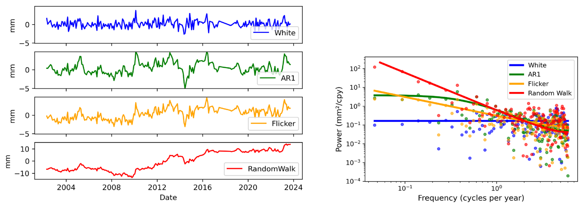
Figure 1 Synthetic GRACE-like time series and corresponding power spectral densities (PSDs) for the stochastic processes considered in this study. Left: synthetic realizations of white noise, AR(1) noise, flicker noise, and random-walk noise; note the different y-axis scale for random-walk noise. Right: empirical PSD (dots) and analytical PSD (lines) of the time series shown in the left panel.

We use the Hector software (Bos et al., 2008, 2021) to estimate the functional parameters of Eq. (2) and the parameters of the selected stochastic model for each grid-cell time series. The variance components and stochastic-model parameters are estimated from the residuals using restricted maximum likelihood estimation (Patterson and Thompson, 1971), which accounts for the loss of degrees of freedom due to the fitted functional model, additionally resulting in more realistic variance estimates (e.g., Gobron et al., 2022). The stochastic-model parameters include the spectral index of the power-law model and the lag-1 coefficient of the AR(1) model. For each grid-cell time series, main quantities are estimated trend $\widehat{b}$ and its uncertainty, represented by the standard deviation ${\mathit{\sigma }}_{\widehat{b}}$, which are used for the significance test and volumetric aggregation.

2.2.2 Significance testing

We apply the significance test under the assumption that the estimated trend is approximately normally distributed. Residual-distribution diagnostics for TWS and GWS, combined over all grid cells, are provided in Fig. S3 in the Supplement. To test whether the estimated trend $\widehat{b}$ from each TWS and GWS time series is significant, we define the null and alternative hypotheses as

$$\begin{array}{}\text{(5)}& {\displaystyle }{H}_{\mathrm{0}}:\text{E}\left(\widehat{b}\right)=\mathrm{0}\text{(6)}& {\displaystyle }{H}_A:\text{E}\left(\widehat{b}\right)\ne \mathrm{0}.\end{array}$$

For each time series and each variable, the test quantity is then formed as

$$\begin{array}{}\text{(7)}& T_b=\widehat{b}/{\mathit{\sigma }}_{\widehat{b}},\end{array}$$

where ${\mathit{\sigma }}_{\widehat{b}}$ is the 1σ standard deviation of the estimated trend, obtained from the corresponding diagonal element of the parameter covariance matrix. Our main results rely on two-sided 99 % confidence levels to reduce false-positive trend detections in the global grid-cell analysis. This results in a significance threshold of $\left|T_b\right|$ = 2.58. The use of this test statistic, and its suitability when ${\mathit{\sigma }}_{\widehat{b}}$ is derived from a calibrated stochastic model, is discussed in more detail by Amiri-Simkooei et al. (2019) and Hohensinn et al. (2024).

2.2.3 Clustering and volumetric aggregation

For the exploratory spatio-temporal analysis in Sect. 3.1, we further apply K-means clustering. K-means clustering is an unsupervised machine-learning algorithm that partitions data into a predefined number of clusters by minimizing within-cluster variance. When being applied to a time-series-populated feature matrix, it iteratively assigns each time series to the nearest cluster (MacQueen, 1967). For the first application, the clustering is used to globally identify dominant TWS and GWS time series patterns. From this result we also use a GWS clustering class as an input for the illustration of significant and non-significant GWS time series. Therefore, we subsequently use another clustering to highlight differences between significant and non-significant time series classes, lying in adjacent regions. The clustering is not used for trend-significance testing or physical attribution.

Significant grid-cell trends are converted to volumetric rates and aggregated into continental and global gain, loss, and net storage-change budgets, as explained in the following: the inputs are the estimated grid-cell trends and trend uncertainties on the downsampled 1° integration grid. Grid centres are assigned to continents using the Natural Earth Admin-0 Countries 1:110m shapefile (ne_110m_admin_0_countries.shp). Grid centres not covered by a country polygon are assigned to the nearest valid land-country polygon; grid-cell areas are computed separately and geodetically on the WGS84 ellipsoid. We use the Natural Earth CONTINENT attribute for all country-to-continent assignments, excluding Russia. For Russia, grid cells west of 60° E are assigned to Europe and those at or east of 60° E to Asia. A grid cell is classified as significant when $\left|\widehat{b}\right|/{\mathit{\sigma }}_{\widehat{b}}$ ≥ 2.58, corresponding to the two-sided 99 % confidence level used above. Only statistically significant grid-cell trends are included in the budgets. Greenland and Antarctica are excluded from both TWS and GWS aggregation. The defined Canadian Arctic Archipelago mask, detailed in Sect. S1.1 in the Supplement, is additionally excluded from the GWS aggregation because residual GWS signals there are especially sensitive to cryospheric leakage and GIA uncertainty; the same cells are retained in the TWS aggregation, where cryospheric mass change is a physically important part of TWS. For comparison, we additionally compute all-cell aggregates from all retained grid cells with finite trend estimates, without significance filtering, and assess GWS-to-TWS ratios under treatment of the Canadian Arctic Archipelago mask (Sect. S1.1).

Grid-cell trends in mm yr⁻¹ equivalent water height are converted to volumetric rates by multiplying with the corresponding grid-cell area:

$$\begin{array}{}\text{(8)}& \mathrm{\Delta }V=\sum _i{A}_i\cdot {\widehat{b}}_i\cdot {\mathrm{10}}^{-\mathrm{6}},\end{array}$$

where ${\widehat{b}}_i$ denotes the estimated grid-cell trend and A_i the grid-cell area in km². The factor 10⁻⁶ converts mm km² to km³, yielding volume-change rates in km³ yr⁻¹, numerically equivalent to Gt yr⁻¹ for freshwater.

Positive and negative significant grid-cell contributions are summed separately to obtain gross gains and gross losses; their sum defines the net storage-change rate. Continental values are obtained by aggregating the significant grid-cell contributions within each continent. Global gain, loss, and net storage-change rates are obtained by summing the corresponding continental contributions. Global mean trends in mm yr⁻¹ are reported as significant-area-weighted means. The procedure is described in more detail in Sect. S1.1.

3 Results

We first use exploratory spatio-temporal and spectral analyses to characterize the dominant variability patterns in the G3P storage time series (Sect. 3.1). We then present the core results, statistically significant TWS and GWS trends and their regional interpretation (Sect. 3.2), followed by the continental and global storage-change budgets and additionally a 95 % threshold assessment (Sect. 3.3). We conclude this part with a discussion on trend significance, model validation and sensitivity to the regression method (Sect. 3.4).

3.1 Exploratory analysis: spatio-temporal and spectral data features

3.1.1 Time-domain clustering

We first use K-means clustering as an exploratory tool to summarize dominant time-series patterns present in the G3P data, and to motivate the choice of the methods presented in the previous section. Clustering is based on the temporal structure of the grid-cell time series and does not use the subsequently estimated trend magnitudes, uncertainties, or significance information. Clusters should not be interpreted as hydrological process classes, but as groups of regions with similar temporal time series behaviour.

The corresponding TWS clustering mainly separates background seasonal/interannual variability, tropical seasonal regimes with different phase and amplitude, moderate depletion-like behaviour, and strong cryosphere-dominated mass loss. The full TWS clustering result is shown and discussed in Sect. S2.1.

Figure 2 shows the exploratory clustering of GWS time series. Compared with TWS, GWS seasonality is generally less pronounced because root-zone soil moisture is removed in the G3P groundwater estimate. Most regions are characterized by background GWS variability or high-latitude seasonal/interannual variability (purple and blue clusters). Moderate GWS drying occurs mainly across mid-latitudes, including large parts of North America and Eastern Europe, and extends into Central and Southern Asia, as well as, to a lesser extent, South America, Southern Africa, and Oceania. The strongest negative behaviour is grouped in the strong GWS decline/cryosphere-adjacent cluster, including northern India and parts of the Canadian Arctic. The northern Indian pattern is consistent with known groundwater depletion from intensive groundwater use, whereas high-latitude signals near the Canadian Arctic require cautious interpretation because they may include leakage from nearby cryospheric mass loss or component-separation artefacts. Positive GWS tendencies occur in parts of Central Africa, South America, the U.S. Midwest and Great Lakes region, Russia, and Central China. The Amazon high-amplitude seasonality cluster remains distinct, reflecting large seasonal groundwater-storage variations.

Figure 2 Exploratory K-means clustering of groundwater storage (GWS) time-series from the G3P data. The map shows the spatial distribution of six clusters, and the sub-panels show the corresponding cluster time series with descriptive cluster names. The black line represents the cluster-mean time series. Units are millimetres of equivalent water height.

Overall, the clustering reveals distinct GWS variability regimes, ranging from widespread background and seasonal/interannual variability to broad mid-latitude drying, localized strong depletion, and regional storage gains, while high-latitude residual signals require cautious interpretation. Formal trend detection and regional interpretation are presented in Sect. 3.2, while volumetric aggregation is presented in Sect. 3.3.

3.1.2 Spectral analysis

To assess data characteristics in the spectral domain and to motivate the stochastic models used for trend uncertainty estimation, we compute Lomb-Scargle periodograms for all time series and for each storage compartment. The resulting globally averaged PSDs, averaged per frequency, are shown in Fig. 3, left panel. We observe pronounced peaks at the annual and semi-annual periods, indicating the substantial contribution of seasonal variability to water storage variations, particularly of RZSM and SWS to contribute to TWS. Further peaks occur at 3 and 4 cycles per year (cpy), corresponding to 4- to 3-month intervals, and additionally at 5 and 6 cpy for some compartment variables, i.e. approximately every second month. When compared with the synthetic examples presented in Fig. 1, all variables show pronounced contributions of coloured, i.e. correlated, noise of both long- and short-range type. This is indicated by higher PSD magnitudes at low frequencies, i.e. long periods, and lower magnitudes at high frequencies, i.e. short periods. The presence of trends still affects the PSDs at long periods.

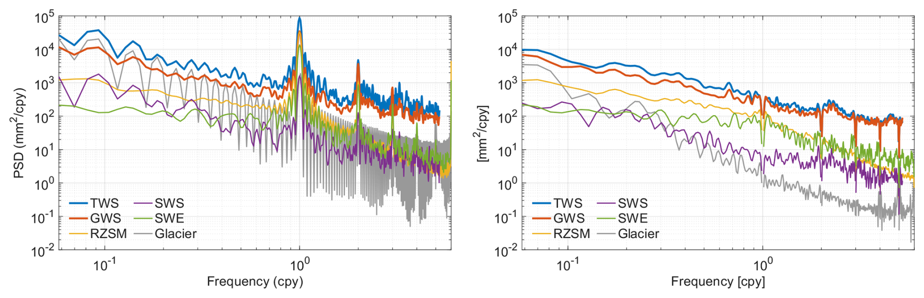
Figure 3 Averaged global power spectral densities (PSDs) of the G3P variables. Left: PSDs of the original time series. Right: PSDs after removal of linear trend and periodic terms by ordinary least-squares regression. TWS: terrestrial water storage; GWS: groundwater storage; RZSM: root-zone soil moisture; SWS: surface water storage; SWE: snow water equivalent; glaciers: glacier mass (GM).

To better assess the influence of trends and seasonal signals, and to reveal the stochastic character of the data, we remove identified periodic seasonal signals (1–6 cpy) and a linear trend using OLS regression. The resulting PSDs of the residuals (Fig. 3, right panel) mostly reflect inter and intraannual variations and observation-system noise. For TWS, GWS, SWS, and glacier mass, we observe spectra close to constant negative slopes in log-log space, indicating power-law behaviour and long-range dependence. Broad interannual power in TWS and GWS variations, approximately over 2–7-year periods, is largely explained by superposed climate modes: combinations of ENSO-, PDO-, and AMO-related effects account for 20 % to 70 % of interannual TWS variability in global basins, with interannual amplitudes of ∼ 10 cm equivalent water height (Pfeffer et al., 2022). The observed power-law spectra of GWS are consistent with long-memory groundwater dynamics, as also found in multi-decadal groundwater-level records that exhibit fractal, power-law scaling and long-range persistence (Li and Zhang, 2007; Little and Bloomfield, 2010).

The spectra of SWE and RZSM tend to flatten at long periods, indicating AR(1)-type, i.e. short-range memory, behaviour. RZSM residuals are well described by AR(1)-type exponential memory, with slightly stronger persistence in drier regimes (Orth and Seneviratne, 2012). SWE anomalies exhibit strong within-season persistence, consistent with short-range memory behaviour (Sospedra-Alfonso et al., 2016), which is also identifiable from our SWE spectrum. In contrast, PSDs of glacier mass and SWS variations indicate power-law behaviour. Long-range dependence with power-law behaviour has also been shown for global river runoff (Koscielny-Bunde et al., 2006), which is consistent with the influence of storage components with longer memory, such as groundwater and glaciers. Glacier mass anomalies can show power-law behaviour over the analysed frequency band, because multiple slow response times make glaciers a multi-timescale low-pass system (Roe, 2011).

Remaining side lobes in the residual PSDs indicate that a fixed set of sinusoidal terms does not fully capture time-variable seasonal amplitude and phase. Such residual spectral structures are expected for hydrological time series with seasonally modulated storage dynamics, resulting from asymmetric recharge–discharge cycles, secondary seasonal peaks, and data gaps. They are particularly visible around the annual and semi-annual periods and in the 2–4 cpy band. As predominantly the intra-annual band is affected, their remaining effect on trend determination, particularly on uncertainty, is expected to be limited and is partially accounted for through the stochastic model calibration. A more detailed discussion of the component-wise spectral behaviour, including representative GWS and RZSM PSDs before and after removal of periodic and trend terms, is provided in Sect. S2.2.

Our exploratory spectral analysis yields three key findings:

• Trend-related low-frequency power. Differences between the PSDs of the original time series and the residuals show that trend-related low-frequency power is strongest for glacier mass and is also evident for TWS, SWS, and GWS, whereas RZSM and SWE exhibit comparatively weak trend contributions.

• Frequency-dependent component dominance. Across most of the analysed frequency range, GWS exhibits the largest spectral amplitudes among the individual storage components and therefore constitutes the dominant storage-component signal within TWS. Because GWS is obtained by component subtraction, these amplitudes may also include TWS observation errors and variability not represented in the subtracted components. Glacier mass dominates only at the very lowest frequencies, which results from strong trend contributions. Among the modelled non-groundwater components, RZSM has the largest spectral amplitudes across much of the seasonal-to-interannual frequency range.

• Variability and memory regimes. The residual spectra indicate long-memory behaviour for TWS, GWS, SWS, and glacier mass, and short-range persistence for RZSM and SWE. The detailed comparison of GWS and RZSM (Sect. S2.2) further shows that RZSM is dominated by seasonal periodic variability, whereas GWS exhibits a pronounced persistent inter-annual variability after removal of the functional signals.

Based on these spectral characteristics, we use power-law-plus-white-noise models for TWS, GWS, SWS, and glacier mass, and first-order-autoregressive-plus-white-noise models for RZSM and SWE when estimating trend uncertainties.

3.2 Global trends in TWS and GWS, and their significance

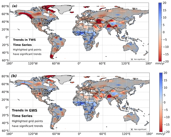
As explained in Sect. 2, we fit trends and trend uncertainties to each TWS and GWS grid-cell time series. For the stochastic component, we use power-law-white-noise models as identified in Sect. 3.1. Figure 4 represents the core results: along with the estimated trends, it highlights the significant trends at the 99 % confidence level in TWS (top) and GWS (bottom). Trends in the other G3P storage components (glacier mass, RZSM, SWS, SWE) are shown in Fig. 5, for which also the identified stochastic processes have been fitted. Maps of estimated TWS and GWS trends without significance-shading can be found in Figs. S4 and S5, Sect. S2.4 in the Supplement. The same figures also discuss stochastic properties (power-law coefficients and trend uncertainties) of the TWS and GWS data, which further support the choice of our models. Figure S6 compares histograms of the parameters shown in Figs. S4 and S5, for TWS and GWS. The median trend uncertainty is lower for GWS than for TWS (2.59 versus 3.86 mm yr⁻¹), which is consistent with the reduced low-frequency persistence after component separation (Fig. S6, middle panel).

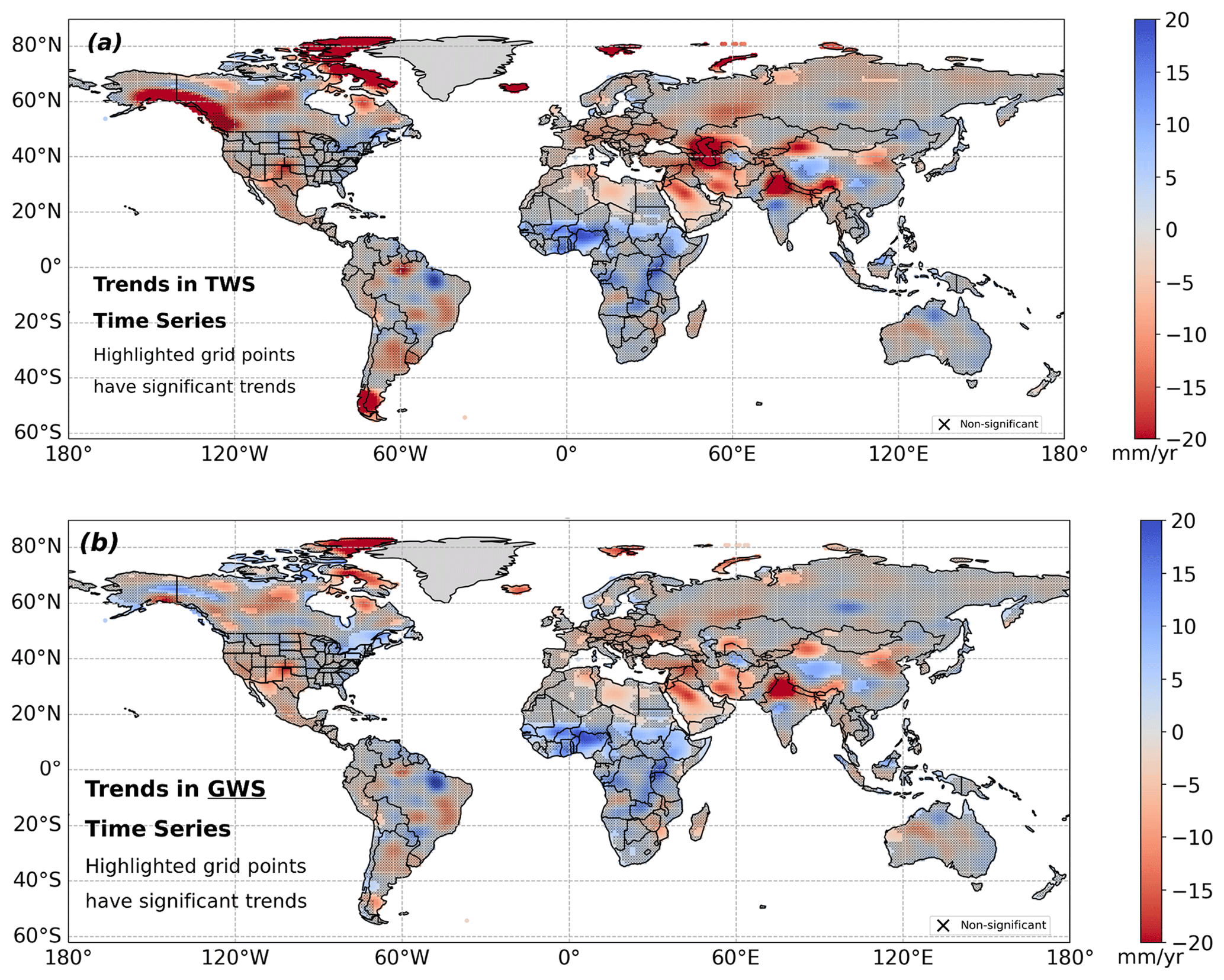
Figure 4 Central result of the global trend analysis: significant G3P TWS (a) and GWS trends (b) under consideration of the calibrated time series models introduced in Sect. 2, and the statistical test. Shading with “X” represents data with insignificant trends, while all non-shaded trends represent statistically significant trends.

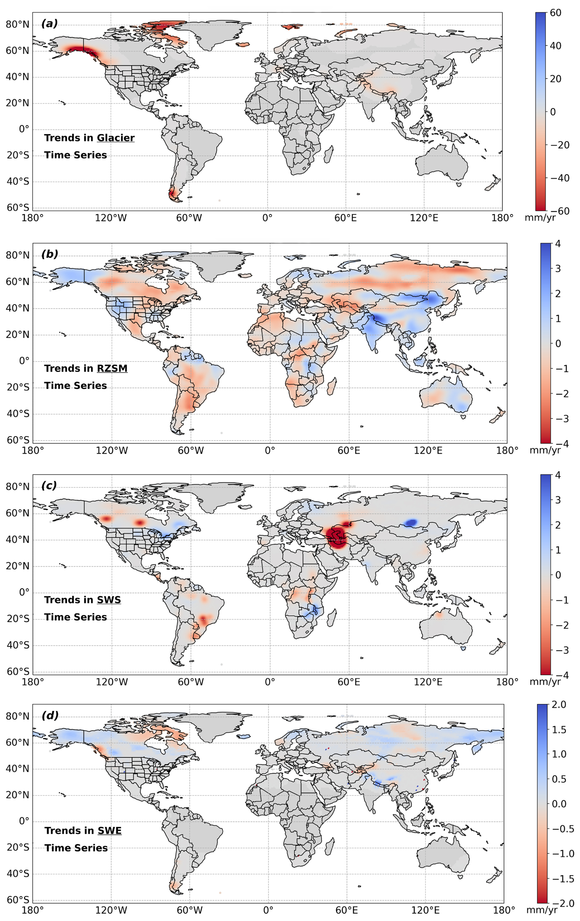
Figure 5 Global trends in glacier mass (a), RZSM (b), SWS (c), and SWE (d). Note that colorbar limits differ among panels.

In the following, we discuss the main TWS and GWS trend patterns shown in Fig. 4, ordered by continent and region. Where relevant, we relate these patterns to the component trends in RZSM, glacier mass, SWS, and SWE shown in Fig. 5, and to the auxiliary fitting parameters presented in the Supplement.

At the global scale, the strongest significant TWS declines coincide with regions of strong ice and glacier mass loss, including Patagonia/Southern Andes, Alaska, and Arctic islands, consistent with earlier work (Velicogna, 2009; Wouters et al., 2019; Braun et al., 2019; Ciracì et al., 2020). In the G3P glacier component (Fig. 5a), glacier retreat dominates low-frequency TWS decline in Canada, Alaska, the Arctic, Patagonia, and the Himalaya, reaching magnitudes up to ∼ −100 mm yr⁻¹. GRACE-derived glacier mass budgets similarly show strongly negative trends, e.g., in Alaska, Patagonia, Arctic Canada, Svalbard and the Russian Arctic, in total summing to ∼ 199 km³ yr⁻¹ over 2002–2016, excluding Greenland and Antarctica (Wouters et al., 2019). Additional prominent negative TWS trends are associated with drought and water depletion, including regions with possible or partial direct human impact (Rodell et al., 2018), and with long-term declines in the Aral and Caspian basins driven by irrigation diversion in the Aral region and regional aridification and enhanced evaporation in the Caspian region. In contrast, the significant GWS trends highlight non-cryospheric freshwater-storage changes, dominating other TWS declines. Major negative GWS patterns occur in intensively managed or semi-arid aquifer regions, including northern India, the North China Plain, Southwest/Central Asia, the High Plains Aquifer, parts of the southwestern US and northern Mexico, and North African fossil aquifer systems. Notably, positive GWS tendencies are most prominent in parts of the Sahel, the Niger Basin, Central/East Africa, and selected mid-latitude regions. Apparent GWS declines in Arctic and ice-adjacent regions require careful interpretation because residual leakage from cryospheric mass loss, GIA uncertainty, and imperfections in the subtracted storage components can propagate into the residual GWS estimate.

3.2.1 North America

For North America, our analysis separates four main regimes: cryosphere-dominated TWS decline in Alaska and Arctic Canada; significant non-cryospheric GWS losses in semi-arid and intensively managed aquifer regions; positive or weakly positive storage tendencies around the Great Lakes and eastern Canada; and regions where apparent TWS trends remain non-significant because of strong interannual variability and large trend uncertainty.

Alaska, Yukon, and the Canadian Arctic

The strongest significant TWS declines in North America occur near the Gulf of Alaska and the Canadian Arctic Archipelago, where they primarily reflect glacier and ice-mass loss (Rodell et al., 2018; Wouters et al., 2019). Outside the strongly glaciated regions, negative TWS and locally significant GWS trends in parts of the Mackenzie and Yukon basins are identified, consistent with permafrost-thaw-related hydrological change, and including increased groundwater connectivity and discharge and associated changes in soil moisture, surface water, and evapotranspiration (Lin et al., 2022; Wright et al., 2022).

The GWS pattern across Alaska and Yukon is spatially heterogeneous. Coastal negative anomalies may reflect residual leakage from the strong glacier-mass signal, whereas localized positive GWS tendencies of approximately +5 to +10 mm yr⁻¹ extend across parts of central Alaska, Yukon, and the Yukon–Kuskokwim lowlands. Their contrast with groundwater losses reported for earlier periods may reflect temporal changes, product and processing differences, or limitations of the storage-component separation in glaciated and permafrost-dominated regions (Muskett and Romanovsky, 2011; Lin et al., 2022). Localized positive TWS and GWS tendencies also occur across parts of the western Canadian Arctic Archipelago, largely outside the regions of strongest glacier mass loss (Noël et al., 2018; Gardner et al., 2011). Because these areas are nevertheless affected by active permafrost degradation and thermokarst processes (Lewkowicz and Way, 2019; Fraser et al., 2018), the mechanisms underlying the positive trends remain uncertain.

In the eastern Canadian Arctic Archipelago, particularly the Queen Elizabeth Islands, significant apparent GWS declines of approximately −5 to −20 mm yr⁻¹ require particularly careful interpretation. They may be influenced by leakage from Greenland and local ice-mass loss, errors in the GIA correction, or imperfections in the subtracted storage components. These high-latitude regions therefore represent GWS sensitivity zones where strong TWS trends, dominated by ice mass loss, cannot be directly attributed to groundwater depletion. These map-level GWS tendencies are retained in the spatial figures for interpretation, but all grid cells falling inside the defined mask (Sect. 2) are excluded from the volumetric GWS aggregation.

Western and central Canada

In the Canadian Prairies, particularly Alberta and the Saskatchewan River Basin, negative TWS tendencies are often not statistically significant because of strong interannual and persistent low-frequency variability and the resulting large trend uncertainties (cf. Sect. S2.4, Fig. S4). GWS, in contrast, shows more spatially coherent and locally significant declines. The shift of power-law κ values of the GWS series relative to TWS (Fig. S6) indicates reduced low-frequency variability after the component-separation step. This TWS–GWS contrast is one of the main regional findings for North America: groundwater-related drying can be detected more distinctly than total-storage decline where TWS is dominated by interannual variability. The GWS pattern is broadly consistent with groundwater abstraction under semi-arid conditions and recurrent drought (Hamdi and Goïta, 2023; Wang et al., 2025).

Similar drying patterns occur around Great Slave Lake and towards the Hudson Bay region. In discontinuous-permafrost regions, thaw can enhance groundwater connectivity, subsurface drainage, and river discharge (Wright et al., 2022; Huang et al., 2025). Northern Quebec and adjacent regions also show a transition from previously reported wetting toward widespread drying, consistent with recent continental assessments (Li et al., 2016; Wang et al., 2025). However, GIA-model uncertainty is substantial around Hudson Bay and can affect both TWS and residual GWS trend magnitudes and, locally, their signs (cf. Sect. 3.2.7).

Great Lakes and eastern Canada

In the Great Lakes Basin, positive TWS tendencies are consistent with the observed transition from record-low water levels in 2013 to record highs by 2017 (Gronewold and Rood, 2019). The corresponding GWS tendencies are positive but not statistically significant. This differs from the GWS decline reported for 2002–2009 by Huang et al. (2012), plausibly because the longer study period includes the pronounced post-2013 lake-level recovery.

Localized significant positive TWS and GWS trends also occur across parts of eastern Canada, including southern Quebec and the Ottawa Valley, and may reflect increased precipitation and groundwater recharge under cold and humid climatic conditions (Dubois et al., 2022). Their contrast with negative trends reported for some eastern Canadian regions over shorter periods (Fatolazadeh and Goïta, 2021) may arise from differences in study period, spatial resolution, GIA correction, or signal processing.

Southwestern US, High Plains Aquifer, and northern Mexico

The clearest non-cryospheric GWS-depletion regime in North America extends across the southwestern US, the High Plains Aquifer, northern Mexico, and the Mexico City region. Significant TWS and GWS declines across New Mexico, Arizona, and the High Plains reflect groundwater abstraction for irrigation coupled with recurrent drought (Scanlon et al., 2012; Konikow, 2015; Jasechko et al., 2024). In the High Plains Aquifer, local GWS trends exceed −20 mm yr⁻¹, reflecting the documented long-term depletion of the aquifer (Haacker et al., 2016).

Component-level interpretation

The component trends assist in distinguishing groundwater-related change from snow, surface-water, and soil-moisture contributions. SWE decreases across southwestern Canada and the Canadian Pacific Northwest and also in parts of the eastern and northern Hudson Bay drainage regions (Fig. 5d). In contrast, slightly positive SWE tendencies occur in parts of the Yukon and Mackenzie basins, indicating that their negative TWS tendencies are not explained by declining snow storage alone. SWS exhibits distinct basin-scale changes, including negative tendencies around Williston Lake and Lake Winnipeg, weaker negative tendencies around Great Slave and Great Bear Lakes, and positive tendencies in the Great Lakes and southern Quebec. These patterns reflect reservoir regulation, changing precipitation and flooding regimes, and observed lake-level variability (Shrestha et al., 2012; Beltaos and Peters, 2024; Kayastha et al., 2022). RZSM decreases across substantial parts of central and western Canada, supporting the interpretation of regional drying associated with changing precipitation regimes and recurrent drought (Bonsal et al., 2019); in northern regions, these changes may interact with permafrost-thaw-related drainage and enhanced hydrological connectivity (Wright et al., 2022). Thus, the Canadian TWS pattern reflects contributions from several storage components, while the more spatially coherent GWS losses identify regions in which groundwater-related drying is particularly pronounced.

3.2.2 South America

Despite locally high-magnitude trend estimates, TWS and GWS exhibit few statistically significant trends across most of South America. More negative power-law κ values, locally approaching random-walk behaviour, indicate strong persistent low-frequency variability and correspondingly large trend uncertainties (Sect. S2.4, top and middle panels of Figs. S4 and S5). The main exceptions are the cryosphere-dominated TWS decline in Patagonia and localized significant GWS depletion in the northern Altiplano and adjacent Andean drylands. Our analysis therefore separates these localized groundwater losses from extensive regions where strong interannual and persistent low-frequency variability prevents the reliable detection of long-term trends. This contrast is particularly evident when GWS is considered separately from the well-documented cryospheric TWS decline in Patagonia.

Altiplano and Andean drylands

The clearest significant GWS declines occur in the northern Altiplano, centred around La Paz and extending westward across the Peru–Bolivia–Chile tri-border region, with local trends reaching approximately −10 mm yr⁻¹. These declines are spatially consistent with regions affected by groundwater stress related to agriculture and mining (Gonzales et al., 2025; García-Sanz et al., 2021).

Farther south, parts of the Andean “Lithium Triangle” across northern Argentina, southwestern Bolivia, and northeastern Chile show localized low-magnitude positive GWS trends instead of a principal depletion signal. Freshwater inputs in these basins are low (2–33 mm yr⁻¹), even as brine and freshwater are extracted (Kirshen et al., 2025). The positive residual GWS tendencies may reflect spatial and temporal variability in recharge, differences between freshwater and brine-storage signals, or limitations of the storage-component separation. This should therefore not yet be interpreted as evidence that mining-related extraction has no hydrological effect.

Patagonia

The strong TWS decline in Patagonia is primarily associated with the well-documented loss of glacier and ice mass (Braun et al., 2019). The corresponding GWS pattern is spatially offset, including positive tendencies in northwestern Chubut and negative tendencies in northeastern Santa Cruz. Its limited spatial correspondence with the glacier component suggests that these GWS tendencies do not simply spatially match the dominant cryospheric TWS signal. However, their interpretation remains sensitive to leakage and uncertainty in the separation of the storage components.

Amazon, La Plata, and São Francisco basins

Across the Amazon, La Plata, and São Francisco basins, most apparent TWS and GWS trends are not statistically significant after accounting for strong interannual and persistent low-frequency variability, with more negative power-law κ values locally approaching random-walk behaviour (Sect. S2.4). Non-significance is therefore an important result: visible regional tendencies cannot generally be distinguished from stochastic storage variability over this study's data period. In the Amazon Basin, the estimated trends form a dipole-like pattern, with negative tendencies in the north and pronounced positive tendencies near the delta, but neither constitutes a pronounced basin-wide trend. Although a basin-mean tendency is broadly compatible with previously reported storage gains, it is not statistically significant in our analysis. Strong ENSO events and subsequent recovery periods contribute substantially to the observed variability (Chaudhari et al., 2019; Satizábal-Alarcón et al., 2024). Similarly, drought-related storage losses previously reported for the southern La Plata Basin, particularly during 2002–2009 (Chen et al., 2010), do not remain significant over the full study period. This can be consistently interpreted with the episodic character of regional drought and with spatially uneven and partial recovery during subsequent periods (Naumann et al., 2023). In the São Francisco Basin, independent evidence for reductions in streamflow and groundwater-supported baseflow (Lucas et al., 2021; de Melo and Wendland, 2020) is likewise not expressed as a spatially extensive significant GWS trend in our analysis.

Component-level interpretation

The component trends support regional hydrological drying without implying widespread significant groundwater depletion. RZSM decreases across central South America, including Bolivia, northeastern Argentina, Uruguay, Paraguay, and southern to southwestern Brazil (Fig. 5). While future projections indicate possible soil-moisture increases in southeastern South America (Lai et al., 2023), historical multi-product assessments show substantial regional variability and drying tendencies over recent decades (Saito et al., 2025; Hirschi et al., 2025). SWS also decreases in the broader São Francisco region, which is consistent with recurrent drought and documented reductions in streamflow and baseflow (Lucas et al., 2021; de Melo and Wendland, 2020). Negative SWS tendencies around Uruguay and Paraguay likely reflect recurrent drought conditions in the La Plata Basin (Chen et al., 2010; Naumann et al., 2023). These component trends help explain parts of the TWS signal but do not alter the principal GWS result: significant groundwater losses are concentrated in the northern Altiplano and adjacent Andean drylands, while parts of the Lithium Triangle show localized positive residual GWS tendencies. Significant long-term groundwater trends remain limited across most of the continent.

3.2.3 Europe

Our analysis indicates a broad but mostly moderate GWS drying tendency across Europe. At the primary 99 % significance level, negative GWS trends are spatially localized, particularly in eastern France, southern Ukraine, and northeastern Spain, which is broadly consistent with previously identified Euro-Mediterranean groundwater-depletion regions (Xanke and Liesch, 2022). Europe provides a useful example of moderate negative trends whose detected spatial extent depends on the significance threshold: At the 95 % threshold, the negative GWS pattern becomes substantially more spatially coherent, extending from northeastern Spain across large parts of France into Germany and the Alpine region (to be discussed in Sect. 3.3). The 99 %-significant trends are therefore embedded within a broader negative pattern that becomes apparent when the significance threshold is slightly relaxed.

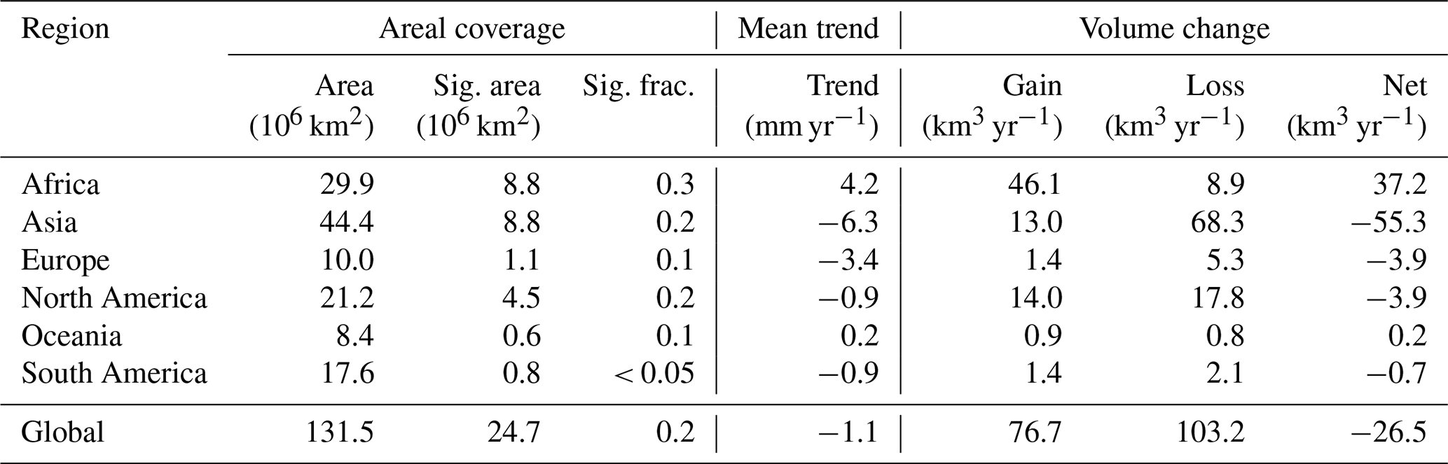
An important feature is that significant GWS trends cover a larger part of Europe than significant TWS trends at both thresholds. At 99 %, significant GWS trends cover 1.1 million km², compared with 0.8 million km² for TWS (Tables 2 and 1). At 95 %, the corresponding areas increase to 2.2 and 1.3 million km², respectively (Tables S1 and S2 in the Supplement). Thus, the broader GWS drying pattern is detected more consistently than the corresponding TWS pattern, despite the generally moderate magnitude of the GWS trends.

Table 1 Significance-filtered TWS trend and water budget statistics by continent. Significant trends computed by $\left|\mathrm{trend}\right|/\mathit{\sigma }$ ≥ 2.58, corresponding to the 99 % confidence level. The mean trend is the area-weighted mean over significant grid cells, and Net = Gain − Loss.

Table 2 Significance-filtered GWS trend statistics by continent. Significant trends computed by $\left|\mathrm{trend}\right|/\mathit{\sigma }$ ≥ 2.58, corresponding to the 99 % confidence level. The mean trend is the area-weighted mean over significant grid cells, and Net = Gain − Loss.

Localized positive GWS trends occur in Denmark, coastal southwestern Finland, Estonia, and coastal western Norway. These may reflect regional recharge variability, but direct attribution is beyond the scope of this study. In northern and coastal regions, component-separation errors and uncertainty in the GIA correction may additionally affect the residual GWS signal.

Relation between TWS and GWS

Across many non-glaciated parts of Europe, TWS and GWS trends show broad spatial correspondence, suggesting a substantial groundwater contribution to regional TWS change. Significant declines in both quantities occur particularly in southern Scandinavia and the northern UK, while the broader GWS drying pattern is consistent with previous GRACE-based groundwater assessments (Xanke and Liesch, 2022). The central Scandinavian decline may indicate a reversal relative to the wetting reported for 2002–2011 (Wang et al., 2013). The northern UK signal is less prominent in previous GRACE syntheses and is only partly consistent with reported in situ groundwater declines, which were mainly identified farther south (Jackson et al., 2015). The larger spatial extent of significant GWS trends, despite their smaller magnitude, likely reflects reduced temporal variability after removal of the other storage components. In TWS, seasonal and interannual variability from soil moisture, snow, and surface water increases trend uncertainty and can obscure moderate long-term groundwater-related changes. Because GWS is derived by component subtraction, however, this greater statistical detectability should not be interpreted as inherently lower physical uncertainty. The different spatial extent of significant TWS and GWS trends also highlights that trend magnitude does not imply statistical significance. At 99 %, the significant European TWS cells have an area-weighted mean trend of −17.0 mm yr⁻¹ and a net change of −13.1 km³ yr⁻¹, substantially more negative than the corresponding GWS values of −3.4 mm yr⁻¹ and −3.9 km³ yr⁻¹ (Tables 1 and 2). The strong TWS aggregate is therefore produced by a smaller significant area with comparatively large negative trends (e.g., Iceland), whereas the GWS drying signal is weaker in magnitude but significant over a larger area.

Component-level interpretation and high-latitude sensitivity

The component trends help explain this contrast. RZSM shows weak-to-moderate drying over Iberia, consistent with recurrent drought conditions (Spinoni et al., 2016), while SWS trends are mostly weak. SWE shows small positive tendencies in the north and negative tendencies farther south. Negative glacier trends over Norway and the Alps are consistent with accelerated glacier mass loss (Zemp et al., 2019; Ciracì et al., 2020). Because the adopted European domain also includes high-latitude cryosphere- and GIA-sensitive regions, the strongly negative continent-wide TWS aggregate cannot be interpreted as groundwater dominated without an additional cryosphere-specific analysis.

In Fennoscandia and the British Isles, uncertainty in the GIA correction can affect both TWS and residual GWS trend magnitudes and, locally, their signs. GWS carries the additional uncertainty of the component-separation procedure, while leakage from glacier mass loss may further affect signals in western Norway. Northern Europe should therefore be regarded as an artefact-sensitive region, in the same sense as discussed for northern Canada.

3.2.4 Africa

Our analysis reveals one of the clearest continent-scale contrasts in GWS: statistically significant depletion across northern Africa is opposed by widespread positive GWS trends extending from the Sahel and Niger Basin into parts of central and eastern Africa. Localized declines additionally occur in southeastern Africa and Madagascar.

Northern Africa

Statistically significant, predominantly moderate, but large-scale GWS declines extend across Algeria, Tunisia, Libya, northern Chad, and northern Egypt. The spatial pattern is consistent with depletion of the North Western Sahara Aquifer System (NWSAS) and Nubian Sandstone Aquifer System (NSAS) reported in previous modelling and GRACE-based assessments (Goncalves et al., 2013; Frappart, 2020; Springer et al., 2023; Shalby et al., 2023), now demonstrated to be significant. Groundwater pumping is commonly identified as the principal driver, although atmospheric water-balance variability may also contribute, particularly in the NWSAS. The broader pattern is also consistent with the high-resolution GRACE TWS trend analysis of Kvas et al. (2024). Despite a considerable natural variability previously reported for African TWS (Rodell et al., 2018; Ni et al., 2018), the northern African GWS-depletion signal remains persistent under our stochastic significance assessment.

West Africa and the Sahel

Pronounced significant positive GWS trends, locally exceeding +20 mm yr⁻¹, are concentrated in the Niger Basin and surrounding Sahelian regions. These trends agree with previous reports indicating groundwater increases in the Sahel and are consistent with enhanced recharge associated with rainfall variability, land-use change, and the so-called “Sahelian paradox” (Werth et al., 2017; Favreau et al., 2009; Felfelani et al., 2017; Ahmed and Wiese, 2019; Springer et al., 2023). Co-located positive TWS trends support the presence of a net regional water-storage increase, although the partitioning among storage components remains model-dependent. The available data are insufficient to attribute GWS gains to a single recharge mechanism.

Central and East Africa

Central Africa exhibits greater spatial heterogeneity. Non-significant negative tendencies occur in parts of the Congo Basin, whereas significant positive GWS trends are found around Chad and Sudan (in the Sahelian zone) and Cameroon. These spatial contrasts may reflect the combined influence of subsurface storage variability and large-scale climate modes, including ENSO and the Indian Ocean Dipole (Jiang et al., 2021; Jarugula and McPhaden, 2023).

In the broader northern East African region, significant positive GWS trends are concentrated across parts of South Sudan, large parts of Ethiopia, and Somalia. Farther south, strong interannual variability limits trend detection (Boergens et al., 2024; Anyah et al., 2018), see Sect. S2.4, Fig. S5. Although pronounced trends characterize these regions, the absence of widespread significant trends is therefore a result of the stochastic behaviour under long memory, as it is the case for Uganda, for example.

Southern Africa and Madagascar

Southern Africa shows predominantly weak positive or non-significant GWS tendencies, interrupted by localized declines in southern Mozambique and Madagascar. These negative trends are spatially consistent with regions affected by recurrent drought (Hoell et al., 2017; Spinoni et al., 2014). Drying tendencies over southern Angola and Namibia are more evident in RZSM than in GWS, indicating that regional drying is expressed more clearly in soil moisture than in groundwater storage.

Component-level interpretation

Across Africa, GWS also explains a substantial part of the large-scale TWS trend pattern, particularly the contrast between northern depletion and Sahelian and East African gains (cf. Figs. S4 and S5). The component trends nevertheless show important regional differences. RZSM decreases in northwest Africa, consistent with declining Mediterranean precipitation and increasing drought frequency (Schilling et al., 2020; Hirschi et al., 2025), and also shows drying over southern Angola and Namibia (Cook et al., 2020; Hirschi et al., 2025). Additional RZSM drying tendencies in parts of central Africa remain uncertain and require validation with independent products.

SWS trends are spatially heterogeneous, with negative tendencies around Lakes Tanganyika and Victoria and positive tendencies around Lake Malawi. The former contrast with documented lake-level rises during 2019–2021, which could be the result of strong multi-annual variability and sensitivity to the analysed period (Gbetkom et al., 2024). To date, no independent observational evidence supports the reported Lake Malawi trend.

3.2.5 Asia

Asia contains the largest continental net GWS loss and one of the most extensive significant groundwater-depletion patterns identified in our analysis. Major depletion regimes extend across Southwest and Central Asia, northern India, the North China Plain, and the Tarim Basin. Localized positive trends occur in western India, the Yangtze and Sichuan basins, parts of central China, and locally across the Tibetan Plateau. The observed continental pattern confirms wide-area groundwater losses, primarily caused by depletion, but also reveals regional contrasts related to groundwater recharge, reservoir-related storage effects, and climate variability.

Southwest and Central Asia

Significant GWS declines of approximately −8 to −10 mm yr⁻¹, with localized hotspots below −20 mm yr⁻¹, occur across the Arab–Persian region. Their spatial extent is consistent with previous GRACE-based evidence of groundwater depletion widely attributed to irrigation-driven abstraction under limited recharge (Joodaki et al., 2014; Nikraftar et al., 2024). Countries most affected by negative trends are Saudi Arabia, Iran and Afghanistan. Notably, significant positive TWS and GWS trends occur across large parts of Turkmenistan. Their co-location coincides with the irrigation-induced regional redistribution of water storage (e.g., Gafurov et al., 2024).

Farther north, strong TWS and SWS declines dominate the Caspian and Aral Sea basins. Caspian Sea losses result from increased evaporation and aridification (Chen et al., 2017), whereas the Aral Sea signal reflects the long-term effects of irrigation and increasingly dry climatic conditions (Wang et al., 2018). Significant negative GWS trends around the Aral Sea, locally reaching approximately −12 mm yr⁻¹, may indicate groundwater depletion associated with irrigation. Although we observe a spatial separation, their attribution remains uncertain as errors in separating the large SWS signal can propagate into GWS.

South Asia

Northern India forms one of the strongest global GWS-depletion hotspots, with local trends approaching −40 mm yr⁻¹. The spatial pattern is consistent with unsustainable irrigation pumping documented by previous GRACE and groundwater studies (Rodell et al., 2009; Dangar et al., 2021). Significant negative GWS tendencies also extend eastward across parts of eastern India and Bangladesh, indicating that the broader depletion pattern is not restricted to the northwestern Indo-Gangetic Basin, contributing to the heterogeneous nature of observed continental water storage patters.

In contrast, positive GWS trends of approximately +10 mm yr⁻¹ occur near Surat in Gujarat and extend eastward. These trends are broadly consistent with previously reported groundwater refilling in parts of western India and with the influence of monsoon-driven recharge variability and water-management interventions (Bhanja et al., 2017; Asoka et al., 2017). South Asia therefore illustrates that significant positive GWS tendencies can occur locally within a region predominantly characterized by depletion.

East Asia

China shows a pronounced spatial contrast in the drivers of significant negative GWS trends. Over the North China Plain and parts of northeastern China, the observed negative significant trend pattern coincides with one of the country's best-documented regions of groundwater over-abstraction, supported by well records, hydrological modelling, and geodetic observations (Cao et al., 2013; Feng et al., 2013; Zhao et al., 2019). Significant GWS losses also extend across Xinjiang and the Tarim Basin, where arid conditions, limited recharge, and irrigation-dominated water use stress groundwater storage. Zhao and Li (2017) reported a slight basin-wide TWS decline and pronounced spatial heterogeneity, but did not isolate the groundwater contribution or attribute the decline specifically to water extraction. In the neighbouring Hexi Corridor, Tangdamrongsub et al. (2017) similarly found declining TWS and GWS during 2002–2010, with the strongest losses in the Shiyang River Basin linked to agricultural water use. By contrast, the negative GWS trends in Yunnan and southwestern China are more consistent with drought and climate variability than with the intensive pumping regimes farther north (Tang et al., 2014). Our results therefore reveal a spatial contrast between well-documented abstraction-related depletion over the North China Plain, irrigation-associated losses in parts of the arid northwest, and declines in Yunnan and southwestern China that are more consistent with drought and climate variability.

Positive residual GWS trends occur in the Sichuan Basin, parts of central China, and locally across the Tibetan Plateau. In Sichuan, these positive tendencies broadly coincide with regions where previous GRACE studies reported increasing TWS (Yao et al., 2016; Cui et al., 2022). However, neither study independently isolated groundwater storage from the other TWS components. Yao et al. (2016) inferred a combined contribution from surface water and groundwater, whereas Cui et al. (2022) identified reservoir storage and climatic factors as major controls. The resulting contrast between depletion in northern and western China and positive trends in parts of central and southern China is a prominent feature of the heterogeneous Asian GWS pattern.

Northern Asia and Arctic Russia

Localized significant negative TWS and GWS trends occur over Taymyr and adjacent Kara Sea regions. These signals may reflect hydrological reorganization associated with permafrost degradation, including enhanced groundwater connectivity and discharge. Such responses have been modelled for the Yukon Flats Basin in Alaska (Walvoord et al., 2012), but their applicability to Taymyr remains tentative. High-latitude leakage, uncertainties in the representation of snow and surface water, and permafrost processes not explicitly represented by the component models can all influence the GWS estimate.

Across northern Russia more broadly, weak-to-moderate negative tendencies are spatially extensive but often not statistically significant. Their non-significance indicates that the apparent drying cannot generally be distinguished reliably from interannual and persistent low-frequency variability over the study period.

Component-level interpretation

The component trends emphasize the strong regional contrasts across Asia. RZSM decreases in the Caspian–Aral region, whereas positive tendencies in northern India and northeastern China may reflect irrigation effects or wetter conditions; these interpretations require further investigation. Extensive RZSM drying across the northern Russian tundra and taiga requires further validation; Chandanpurkar et al. (2025) identified northern Russia as a mega-drying region. However, it did not yet affect GWS or TWS trends to be large-scale significant, which also holds for the 95 % significance case (Fig. S7). Also, its interpretation remains uncertain because Arctic soil-moisture is reported to respond regionally heterogeneous and are affected by changing evapotranspiration, permafrost conditions, and surface-water–groundwater connectivity (Bring et al., 2016).

SWS declines around the Caspian and Aral seas indicate that surface-water loss contributes substantially to the regional TWS decline (Chen et al., 2017; Singh et al., 2012). Broad positive SWE tendencies across Siberia are broadly consistent with station observations showing increasing maximum SWE in parts of western and eastern Siberia, although the observation period and spatial coverage differ from those of the present analysis (Bulygina et al., 2011). Negative SWE trends in the Caucasus and parts of the Central Asian mountains require further validation. Elevated persistent variability in parts of Central Asia, the Middle East, and China increases trend uncertainties and limits the spatial extent of statistically significant trends (Sect. S2.4). These component signals help interpret TWS patterns but do not change the principal Asian GWS result: widespread groundwater depletion is in contrast to significant regional gains and with areas where variability or component-separation uncertainty prevents a clear attribution.

3.2.6 Oceania/Australia

Australia is characterized by a pronounced wet–dry contrast and strong interannual variability rather than by spatially extensive significant GWS depletion. Previous GRACE-based analyses identify repeated storage gains in the tropical north and northeast and persistent deficits across western and southern Australia (Yang et al., 2020). Our component analysis identifies a mild but significant GWS decline in central-western Australia, consistent with GRACE–model fusion studies indicating groundwater-dominated long-term TWS reductions under persistent rainfall deficits (Yang et al., 2020).

In northern Australia, strong precipitation-driven interannual variability limits the detection of persistent long-term trends. GRACE-derived TWS anomalies in this region are closely related to rainfall and vegetation variability (Yang et al., 2014), indicating that episodic wet and dry periods dominate the storage record. The principal finding is therefore not widespread groundwater depletion, but a localized significant GWS decline in central-western Australia embedded within otherwise highly variable and largely non-significant regional patterns.

3.2.7 The role of glacial isostatic adjustment (GIA)

GIA represents an important source of systematic uncertainty in GRACE/GRACE-FO trend analyses, particularly at northern latitudes and in formerly glaciated regions. Using an ensemble-based framework, Eicker et al. (2024) demonstrate that in parts of North America and Fennoscandia the magnitude – and, in some localized cases, also the sign – of GRACE-derived TWS trends can depend on the adopted GIA realization. The strongest sensitivities occur around Hudson Bay and northern Quebec, where GIA gravity-rate signals are large and spatially heterogeneous and GIA-related uncertainty can locally exceed several cm yr⁻¹ equivalent water height.

These regions coincide with areas highlighted in our analysis as requiring cautious interpretation, including northern Canada, parts of the Canadian Arctic Archipelago, Fennoscandia, and the British Isles. Also, Eicker et al. (2024) show that hydrological trend estimates over large parts of Europe and other mid-latitude regions are comparatively less sensitive to the adopted GIA realization. This indicates that GIA uncertainty is particularly important at northern latitudes and in formerly glaciated regions, whereas most mid-latitude continental patterns are expected to be less strongly affected.

Because G3P GWS is derived by component subtraction from TWS, any residual GIA from the GRACE/-FO lower-level processing in TWS propagates directly into the estimated GWS trends. In strongly GIA-affected regions, apparent GWS trends may therefore be biased locally by several mm yr⁻¹, potentially affecting both trend magnitude and statistical significance near the detection threshold. Residual GWS trends in the principal GIA-affected regions thus require particular caution because they combine GIA uncertainty with uncertainty from the storage-component separation. Outside these northern-latitude sensitivity regions, the large-scale continental interpretations are less likely to be much affected by GIA uncertainty and remain broadly consistent with independent hydrological evidence.

3.3 Rates of change, budgets and 95 % sensitivity

Here we present continentally aggregated, area-weighted mean trends and associated volume-change rates derived from G3P grid-cell time series that exhibit statistically significant trends, as described in Sect. 2.2. Unless stated otherwise, continental and global balances in this section refer to the sums of grid-cell volume-change rates passing the specified significance threshold. Gross gains and gross losses are reported as positive magnitudes, and the net volume-change rate is calculated as gain minus loss. Significance is assessed separately for TWS and GWS. Greenland and Antarctica are excluded from both aggregations. The primary TWS aggregation domain retains all eligible grid cells, and the primary GWS aggregation domain excludes signals in parts of the Canadian Arctic Archipelago because these strong GWS trends are particularly sensitive to glacier-signal leakage, GIA uncertainty, and potential limitations in the storage-component models (Sect. 2). Consequently, the areas used for the TWS–GWS ratio analysis differ slightly; we assess this sensitivity separately.

Global 99 % aggregates

Tables 1 and 2 summarise the 99 %-significance-filtered TWS and GWS trend and volume-change statistics by continent and globally.

For TWS, the net global volume-change rate over grid cells with significant trends amounts to −183.4 km³ yr⁻¹. The aggregate is dominated by losses in North America (−90.5 km³ yr⁻¹) and Asia (−89.3 km³ yr⁻¹), with smaller net losses in South America (−16.8 km³ yr⁻¹) and Europe (−13.1 km³ yr⁻¹). Africa shows a net TWS gain of +25.9 km³ yr⁻¹.

For GWS, the corresponding net global volume-change rate is −26.5 km³ yr⁻¹. This net decline is primarily associated with Asia (−55.3 km³ yr⁻¹), with smaller net losses in Europe (−3.9 km³ yr⁻¹), North America (−3.9 km³ yr⁻¹), and South America (−0.7 km³ yr⁻¹). These losses are partly compensated for by a substantial net GWS gain in Africa of +37.2 km³ yr⁻¹. The global gross negative GWS change amounts to 103.2 km³ yr⁻¹.

Global GWS-to-TWS ratios

Using the defined primary aggregation domains, the net negative GWS aggregate of −26.5 km³ yr⁻¹ is approximately 14 % of the net negative TWS aggregate of −183.4 km³ yr⁻¹, while the gross negative GWS change of 103.2 km³ yr⁻¹ is approximately 44 % of the corresponding TWS change of 232.1 km³ yr⁻¹. The substantially smaller net than gross GWS-to-TWS ratio reflects compensation between regions of groundwater loss and gain. At the 99 % threshold, significant GWS gains of 76.7 km³ yr⁻¹ compensate for approximately 74 % of the gross GWS loss, whereas significant TWS gains compensate for approximately 21 % of the gross TWS loss. The comparatively small global net GWS decline therefore does not imply uniformly weak groundwater trends, but partly results from compensation between substantial regional losses and gains, particularly the positive GWS aggregate in Africa.

Sensitivity to the spatial domain

Because the primary TWS and GWS spatial domains differ slightly, we separately tested the sensitivity of these ratios to the treatment of the Canadian Arctic Archipelago. Applying the same exclusion mask used for GWS to TWS reduces its net and gross negative changes to −144.9 and 193.6 km³ yr⁻¹, respectively, yielding corresponding GWS-to-TWS ratios of approximately 18 % and 53 %. Conversely, retaining the excluded Arctic cells in the GWS aggregation increases its net negative and gross negative changes to −35.8 and 112.9 km³ yr⁻¹, respectively. Thus, the primary descriptive GWS-to-TWS ratios are approximately 14 % for net loss and 44 % for gross loss, while the artefact-sensitivity analysis yields ratios of approximately 18 %–20 % and 49–53 %, respectively, depending on the treatment of the Canadian Arctic Archipelago.

Comparison with previous estimates and all-cell results

The gross negative significance-filtered GWS change of 103.2 km³ yr⁻¹ is of the same order of magnitude as earlier model-based estimates of global groundwater depletion of approximately 100–150 km³ yr⁻¹ (Döll et al., 2014). Most of the negative GWS aggregate is concentrated in established groundwater-depletion regions, although climate-driven recharge deficits, drought-related storage changes, permafrost-related processes, and residual component errors contribute locally. Groundwater depletion can itself be intensified by drought through reduced recharge and increased groundwater abstraction, as observed, for example, in the Persian/Iranian region.

As a complementary estimate of storage change, we also integrated all retained grid-cell trends without conditioning on statistical significance (Tables S3 and S4). The resulting global gross negative changes are substantially larger, amounting to 469.4 km³ yr⁻¹ for TWS and 262.6 km³ yr⁻¹ for GWS, corresponding to a gross GWS-to-TWS ratio of approximately 56 %. This all-cell ratio is closer to the 68 % groundwater contribution to TWS loss reported by Chandanpurkar et al. (2025), although differences in spatial domain and methodology remain.

Continental differences

The contribution of groundwater to continental TWS change differs strongly among continents, reflecting both the magnitude and spatial compensation of regional GWS trends. At the continental scale, the largest GWS contribution to significant TWS loss occurs in Asia: the net GWS loss is approximately 62 % of the net TWS loss, and the gross GWS loss approximately 70 % of the gross TWS loss. At the 99 % threshold, significant trends cover approximately one fifth of the analysed Asian area for both TWS and GWS. Africa shows the opposite behaviour, with a net GWS gain of +37.2 km³ yr⁻¹ compared with a net TWS gain of +25.9 km³ yr⁻¹. Significant GWS trends cover approximately 29 % of the analysed African area, compared with approximately 22 % for TWS.

The relation between TWS and GWS is considerably different on the other continents. In North America, the descriptive net GWS-to-TWS ratio is approximately 4 %, rising to about 8 % when both variables are aggregated over the same geographic domain ($\mathrm{3.9}/\mathrm{52.0}$). The comparatively small net GWS loss reflects substantial regional compensation: significant GWS gains of 14.0 km³ yr⁻¹ compensate for most of the gross loss of 17.8 km³ yr⁻¹. Thus, the spatially extensive groundwater-drying pattern does not yet translate into a comparably large continental net loss. Significant trends cover approximately 21 % of the analysed GWS domain and 17 % of the TWS domain. In Europe, significant GWS trends similarly cover a larger fraction of the analysed domain than TWS trends (approximately 11 % versus 8 %). In South America, in contrast, the significant TWS net loss of −16.8 km³ yr⁻¹ is accompanied by only −0.7 km³ yr⁻¹ of net significant GWS change. Thus, the continental TWS loss is not accompanied by a corresponding continent-wide groundwater-storage decline.

95 % sensitivity

Repeating the analysis at the 95 % confidence level using a test threshold of 1.96 (Fig. S7) preserves the principal large-scale TWS and GWS patterns while increasing the spatial extent of trends classified as significant. Globally, the significant TWS area increases from 21.4 to 27.9 million km², corresponding to an expansion of approximately 30 % relative to the 99 % values, while the significant GWS area increases from 24.7 to 33.6 million km², corresponding to a relative expansion of approximately 36 %.

The corresponding changes in the integrated volume-change rates are more moderate. The net global TWS loss increases from −183.4 to −199.7 km³ yr⁻¹ (approximately 9 %), and the gross negative TWS change from 232.1 to 264.5 km³ yr⁻¹ (approximately 14 %). The net GWS decline increases from −26.5 to −31.4 km³ yr⁻¹ (approximately 18 %), and the gross negative GWS change from 103.2 to 128.8 km³ yr⁻¹ (approximately 25 %; Tables S1 and S2). At the same time, the magnitude of the global area-weighted mean trend over significant cells decreases from −8.6 to −7.2 mm yr⁻¹ for TWS and from −1.1 to −0.9 mm yr⁻¹ for GWS. Thus, lowering the significance threshold primarily expands the detected spatial footprint by accepting a broader set of moderate trends rather than substantially altering the storage-change budgets. This increased sensitivity is also accompanied by the expected rise in the nominal false-positive probability from 1 % to 5 %, while at the same time the risk of missing weaker true trends is reduced.

The relative relationships between the global significance-filtered aggregates also change only moderately. The net GWS-to-TWS ratio increases from approximately 14 % to 16 %, while the gross ratio increases from approximately 44 % to 49 %. Compensation between significant gains and losses is likewise stable: at 95 %, GWS gains compensate approximately 76 % of the gross GWS loss, compared with approximately 25 % for TWS, similar to the corresponding 74 % and 21 % values at 99 %. This confirms that the comparatively small net global GWS decline is strongly influenced by compensation between regional groundwater losses and gains.

Regional changes at 95 %

The increase in spatial coverage is particularly evident in Europe. Significant GWS area doubles from 1.1 to 2.2 million km², corresponding to approximately 11 % and 22 % of the analysed European area, respectively. For TWS, the significant area increases from 0.8 to 1.3 million km², or from approximately 8 % to 13 %. Negative GWS trends become more spatially coherent, extending from northeastern Spain across large parts of France into Germany and the Alpine region. The 99 %-significant trends are therefore spatially embedded within a broader moderate negative GWS pattern that becomes apparent when the significance threshold is relaxed.

The main continental contrasts remain stable under the lower significance threshold. In Asia, the significant area increases to approximately 26 % of the analysed continental area for both TWS and GWS. The net GWS-to-TWS ratio changes only from approximately 62 % at 99 % to 60 % at 95 %, while the corresponding gross-loss ratio remains nearly unchanged at approximately 70 % and 69 %, respectively. Africa retains positive net TWS and GWS changes, while the significant areas increase from 6.5 to 8.3 million km² for TWS (approximately 22 % to 28 % of the analysed area) and from 8.8 to 11.3 million km² for GWS (approximately 29 % to 38 %). In North America, the significant-area fractions increase from approximately 17 % to 23 % for TWS and from approximately 21 % to 30 % for GWS. The net significant GWS loss correspondingly increases from −3.9 to −8.6 km³ yr⁻¹. A similar increase occurs in Europe, from −3.9 to −8.5 km³ yr⁻¹, whereas the much larger Asian net GWS loss changes only moderately from −55.3 to −60.8 km³ yr⁻¹. This contrast indicates that the broad moderate drying patterns in North America and Europe are more sensitive to the significance threshold, whereas the major Asian depletion signal is comparatively threshold-stable. In South America, the significant TWS net loss changes only slightly from −16.8 to −17.3 km³ yr⁻¹, whereas the net significant GWS change remains close to zero.

Overall, lowering the significance threshold substantially expands the spatial coverage of detected trends, particularly for GWS and most prominently in Europe, while producing only moderate changes in the integrated storage budgets. The principal continental contrasts – strong and threshold-stable groundwater losses in Asia, compensating groundwater gains in Africa, increasingly coherent moderate GWS drying in Europe, and substantial South American TWS losses without a corresponding continent-wide GWS decline – are preserved. The main spatial patterns and continental-scale volume estimates therefore change little with the selected significance threshold, while the absolute global GWS-to-TWS ratios change little depending on how the artefact-prone Canadian Arctic Archipelago is treated.

3.4 Assessment of trend significance and model evaluation

To examine how trend magnitude and stochastic variability jointly determine trend significance, Fig. 6 shows the estimated GWS trend against its standard deviation for each time-series cluster identified in Fig. 2. Gray-shaded regions denote trends classified as statistically significant, and logarithmic axes are used to improve visibility.

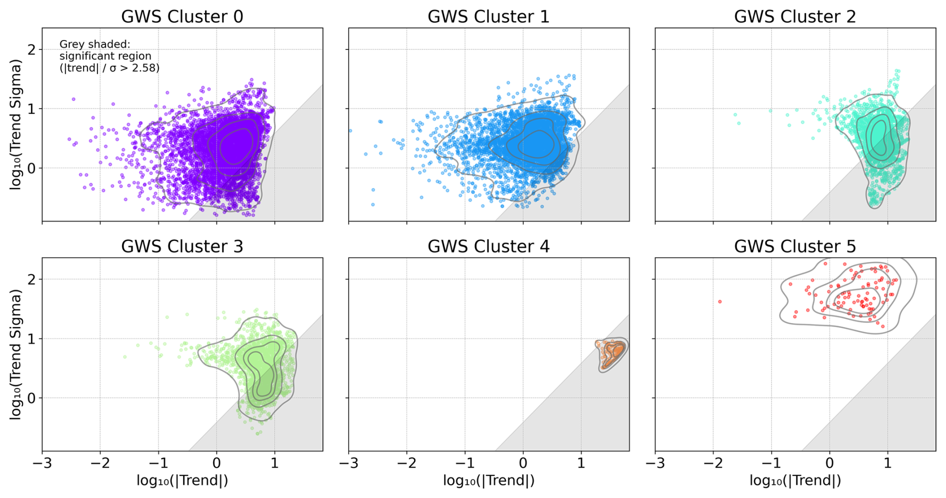
Figure 6 GWS trend magnitude versus trend standard deviation for each time-series cluster identified in Fig. 2. Each dot represents one grid cell; gray-shaded regions denote statistically significant trends. Logarithmic axes are used for better visibility.

The two globally dominant background-variability clusters (clusters 0 and 1; purple and blue) are largely characterized by non-significant trends (Fig. 6, top panels). The same applies to the Amazon high-amplitude seasonality cluster (cluster 5; red), where strong seasonal, interannual, and persistent low-frequency variability produces large trend uncertainties. In contrast, the strong-decline/cryosphere-adjacent cluster (cluster 4; orange), which includes Arctic regions and parts of India, is dominated by significant negative trends with comparatively limited scatter. The positive-GWS-tendency cluster (cluster 3; green) contains spatially widespread groundwater increases across several continents, of which approximately half reach statistical significance. Statistical significance does not, however, lead to unambiguous physical interpretation. This is particularly important for significant residual GWS trends in Arctic and cryosphere-adjacent regions, where leakage, GIA uncertainty, and errors in the modelled storage components can affect the estimated signal.

To investigate the transition between significant and non-significant trends in more detail, we focus on the moderate-GWS-drying cluster (cluster 2; turquoise; top-right panel of Fig. 6), which contains comparable numbers of significant and non-significant time series. Similar to the positive-GWS-tendency cluster, cluster 2 exhibits a similar distribution of trend magnitudes, but with greater variation in trend uncertainty associated with interannual and persistent low-frequency variability. The cluster predominantly contains small-to-moderate negative GWS trends and is therefore well suited for illustrating the sensitivity of significance classification to both trend magnitude and residual variability. Figure 7a shows its spatial distribution, with crosses marking grid cells whose trends are not statistically significant.

To select spatially coherent examples of significant and non-significant time series, we further group the cluster 2 series using K-means, now based on binary trend significance and demeaned geographic latitude and longitude, with all features standardized. We use seven sub-clusters, which provide a practical balance between spatial coherence and interpretability. Because significance is itself included as a clustering feature, this grouping is intended to support visualization and comparison of tradeoffs between significant and non-significant clusters.

The spatial distribution of the resulting sub-clusters is shown in Fig. 7b, and representative time series are presented in Fig. 8. In each panel, the upper series shows the observations after removal of the fitted periodic components for visual clarity, while the lower series shows the residuals from the complete parametric model fit. The panels in the left column show the time series of the significant trend clusters, the panels on the right column show the non-significant clusters.

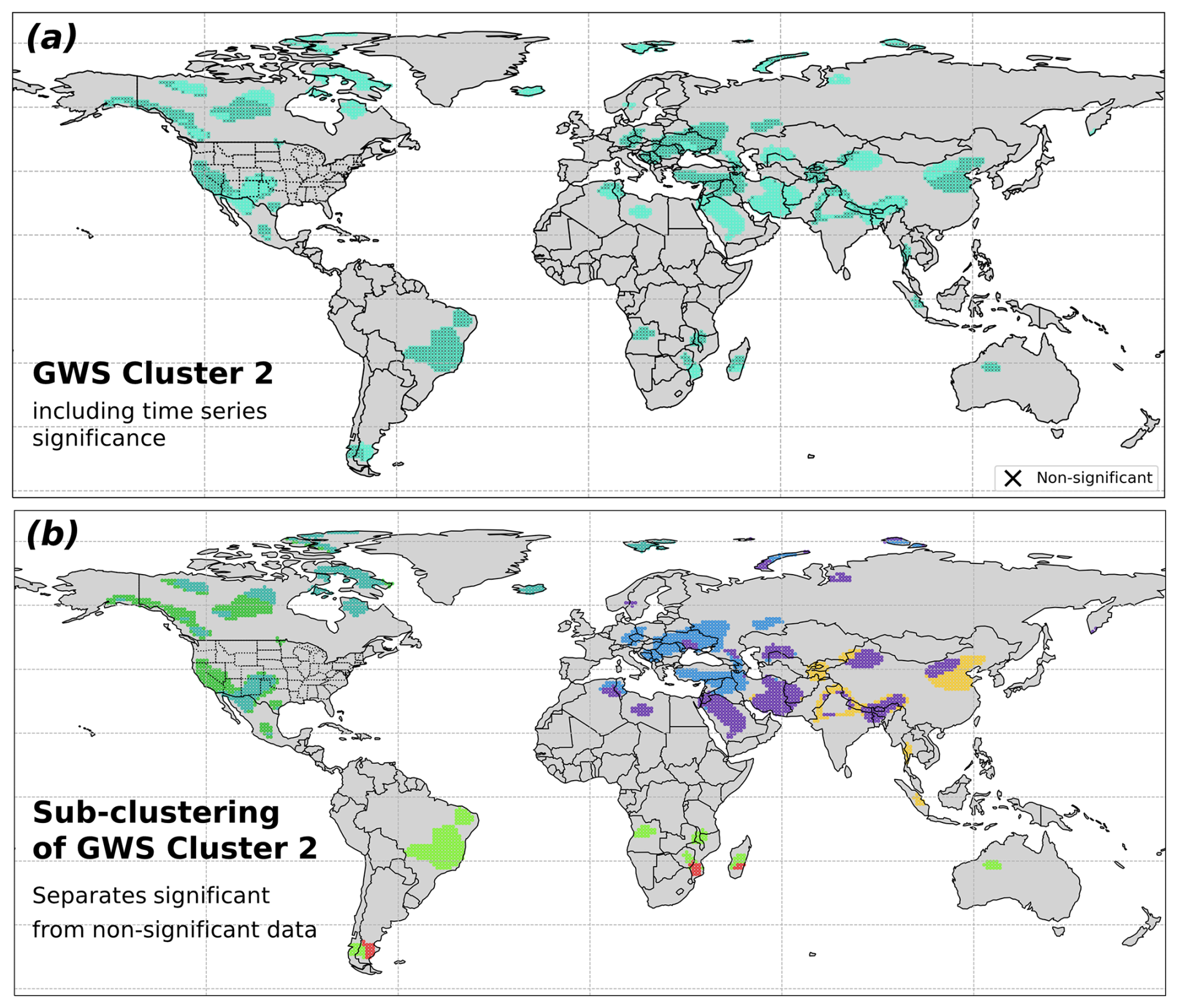
Figure 7 (a) Spatial distribution of GWS cluster 2 from Fig. 2; crosses indicate grid cells with non-significant trends. (b) Sub-clustering based on binary trend significance and geographic location, used to select spatially coherent examples of significant and non-significant time series.

Figure 8 Representative time series corresponding to the sub-clustering of GWS cluster 2 shown in Fig. 7b. The left panels show significant sub-clusters and the right panels non-significant sub-clusters. Observations after removal of the fitted periodic components are shown above the corresponding model residuals.

Comparison of the representative significant and non-significant time series in Fig. 8 illustrates systematic differences in both trend magnitude and residual variability. Significant trends range from approximately −7.1 to −11 mm yr⁻¹, whereas the selected non-significant trends are generally weaker, ranging from approximately −5.1 to −7.1 mm yr⁻¹. The significant examples also exhibit less residual variability, while stronger interannual and persistent low-frequency variations obscure the linear component in the non-significant examples.

In several cases, low-frequency residual variations are comparable to or larger than the fitted linear change. Some time series additionally exhibit weak non-linear behaviour, including slight positive tendencies before approximately 2007. These examples illustrate that trend significance depends jointly on the magnitude of the fitted trend and the stochastic properties of the time series; relatively large apparent trends may remain non-significant when persistent variability produces correspondingly large trend uncertainties.

Further evaluations include comparison of the empirical residual spectra with the fitted stochastic models and an assessment of the sensitivity of GWS trends to the treatment of temporal covariance using OLS and GLS (Sect. S2.6 “Model evaluation and trend sensitivity”). The fitted stochastic models reproduce the low- and intermediate-frequency empirical residual spectra well, including the frequencies most relevant for trend uncertainty. Compared with OLS, GLS yields a slightly narrower and more negative GWS trend distribution and global mean and median shifts of approximately 0.3–0.4 mm yr⁻¹, which indicates the sensitivity to proper covariance modelling. By accounting explicitly for temporal covariance, GLS provides more reliable trend estimates in the presence of persistent interannual variability and is less susceptible to such variability influencing the fitted linear trend, as particularly evident in the latitude-dependent comparison of Fig. S9, e.g., for South America.

(Döll et al., 2014)

Table 3 Summary of the main findings on G3P GWS and TWS trends for 2002–2023.

4 Conclusion and outlook

In this study, we present a globally consistent assessment of terrestrial water storage (TWS) and groundwater storage (GWS) trends using the Global Gravity-based Groundwater Product (G3P) and 21.5 years of GRACE/GRACE-FO observations from 2002 to 2023. Trend and periodic signals are estimated for each grid-cell time series together with a calibrated stochastic model of residual temporal covariance, which allows trend uncertainties to account for interannual variability, hydrological memory, and remaining observational noise. This provides significance-filtered continental and global groundwater gain, loss, and net storage-change estimates, complemented by aggregates over all retained grid-cell trends.

At the 99 % confidence level, significance-filtered net TWS and GWS changes amount to −183.4 and −26.5 km³ yr⁻¹, while gross negative changes reach 232.1 and 103.2 km³ yr⁻¹, respectively. Over the spatial aggregation domains, these correspond to descriptive GWS-to-TWS ratios of approximately 14 % for net change and 44 % for gross negative change; artefact-aware sensitivity tests yield approximately 18 %–20 % and 49 %–53 %, respectively. Integrating all retained grid-cell trends increases the gross negative changes to 469.4 km³ yr⁻¹ for TWS and 262.6 km³ yr⁻¹ for GWS, corresponding to a gross GWS-to-TWS ratio of approximately 56 %. Net balances additionally mask substantial compensating groundwater gains, particularly in Africa.

The principal global, regional, and methodological findings are synthesized in Table 3. Asia accounts for the largest net GWS loss (−55.3 km³ yr⁻¹), with extensive depletion across Southwest and Central Asia, northern India, the North China Plain, and the Tarim Basin. Africa exhibits the largest compensating GWS gain (+37.2 km³ yr⁻¹), with positive trends from the Sahel and Niger Basin into parts of central and eastern Africa despite continued depletion in northern Africa. Broad groundwater drying is also evident across western and central Canada and Europe, whereas persistent variability limits detection of spatially extensive trends across much of South America. Groundwater depletion can additionally be intensified by drought through reduced recharge and increased abstraction, illustrating coupled climatic and anthropogenic controls. GWS trends in GIA-, cryosphere-, surface-water-, reservoir-, and permafrost-affected regions, such as the Canadian Arctic Archipelago, require particular caution and should not be interpreted as groundwater change from statistical significance alone.

Across most of the analysed spectral range, residual GWS shows the largest spectral amplitudes among the individual storage components, including much of the seasonal-to-interannual range, whereas glacier mass dominates trends at the lowest frequencies. Because GWS is derived by component subtraction, it may also contain TWS errors and variability not represented in the subtracted components. Negative GWS tendencies are particularly widespread across the Northern Hemisphere.

Repeating the analysis at the 95 % confidence level preserves the principal spatial and volumetric conclusions. Relative to 99 %, significant area expands by approximately 30 % for TWS and 36 % for GWS, whereas net-loss magnitudes increase by only approximately 9 % and 18 %, respectively. The net GWS-to-TWS ratio changes from approximately 14 % to 16 %, and the gross ratio from 44 % to 49 %. Relaxing the threshold thus primarily expands the spatial extent of detected moderate trends and has only little effect on storage change budgets.

Further evaluations show that trend significance depends jointly on trend magnitude and persistent stochastic variability. Power-law-plus-white-noise models reproduce the low- and intermediate-frequency residual spectra governing long-term trend uncertainty. Separation of modelled non-groundwater components generally reduces low-frequency variability and associated stochastic trend uncertainty, improving GWS detectability, but introduces additional uncertainty from the RZSM, SWS, SWE, and glacier-storage products. Accounting for temporal covariance through GLS yields a slightly narrower global GWS trend distribution shifted by approximately 0.3–0.4 mm yr⁻¹ toward more negative values relative to OLS, with the largest differences in South America. Global water-storage trend estimates therefore remain sensitive to stochastic modelling, product selection, spatial masking, component separation, and significance criteria.

Compared with approaches based primarily on deterministic trend fitting or direct TWS interpretation, the framework combines component-resolved groundwater estimation, calibrated temporal-covariance modelling, and significance-aware volumetric aggregation. This allows long-term trends to be distinguished more effectively from persistent hydrological variability and separates trend magnitude, detectability, and uncertainty explicitly.

The significance-filtered gross negative GWS change of 103.2 km³ yr⁻¹ is of the same order of magnitude as previous model-based estimates of global groundwater depletion (e.g., Döll et al., 2014). The complementary all-cell integration yields substantially larger gross negative changes and a GWS-to-TWS ratio of approximately 56 %, closer to the 68 % groundwater contribution to TWS loss reported by Chandanpurkar et al. (2025). The difference from previous estimates should be interpreted in light of differences in spatial domain, component definition, and aggregation methodology.

Future work should improve characterization of the non-groundwater storage components, particularly RZSM, SWS, SWE, and glacier storage, whose errors propagate directly into residual GWS trends. A more complete uncertainty assessment should jointly account for the reduced stochastic uncertainty achieved through component separation and the additional uncertainty introduced by the component products. Improved leakage treatment and GIA corrections remain particularly important in high-latitude and glacier-dominated regions, while systematic differences between spherical-harmonic and mascon TWS products (Çakan et al., 2025) motivate cross-product trend and uncertainty assessments. Spatially correlated uncertainty in aggregated storage-change estimates and field-wide significance across the global grid also warrant further investigation.

Independent constraints from hydrological models, in situ groundwater observations, and complementary geodetic measurements such as GNSS and InSAR will be important for separating climatic, anthropogenic, and model-related contributions. Longer records from GRACE-C and subsequent mass-change missions, together with explicit measurement-stability uncertainty concepts (Gobron et al., 2026; Merchant et al., 2026) and full use of validated G3P formal uncertainties, should further improve trend detectability and volumetric change estimates.