Non-stationary low-flow frequency analysis with mixed Weibull components and Copula-based dependence framework

Extreme low flows are a pressing challenge for water management, reducing water availability and degrading water quality. Reliable design estimates are therefore essential. Traditional low-flow frequency analysis relies on the assumption of independent and identically distributed (i.i.d.) data, which is increasingly violated under climate change and by varying low-flow generating processes. In a seasonal snow-influenced climate, annual low-flow extremes may occur in both summer and winter, potentially exhibiting seasonal dependence that challenges conventional modelling approaches. This study extends traditional low-flow frequency analysis to non-stationary conditions by jointly accounting for temporal trends, seasonal heterogeneity and inter-event dependence. Building on previously developed mixed distribution and mixed copula frameworks, we generalise these frameworks to non-stationary conditions using three-parameter Weibull distributions. Seasonal low-flow distributions and their joint mixture vary over time, with linear non-stationarity in the location parameter and in inter-event dependence. Results are presented for more than 700 catchments from the European Reference Observatory of Basins for INternational hydrological climate change detection (ROBIN) dataset. Model evaluation shows that neglecting non-stationarity when present can lead to biased assessments of low-flow severity, particularly for higher return periods. In contrast, non-stationary models provide a more realistic representation of evolving low-flow regimes by revealing temporal changes that remain hidden from traditional estimators. By preserving the conceptual consistency of the previous stationary framework, the proposed non-stationary framework improves the statistical characterisation of extreme low flows and provides an enhanced basis for low-flow frequency analysis by offering new insights into past and current low-flow processes under climate change.

1 Introduction

Frequency analysis (FA) is the most straightforward statistical approach for estimating the probability of hydrological extremes. In the context of low-flows, low-flow frequency analysis (LFA) is used to derive design low-flows associated with specific non-exceedence probabilities by fitting probability distributions to characteristic time series, most often annual minimum streamflow (Tallaksen and Laaha, 2023). The reliability of these estimates depends strongly on both sample size and the validity of the underlying model assumptions. Traditional LFA assumes that observations are independent and identically distributed (i.i.d.), implying (i) stationarity of the time series, (ii) homogeneity of the underlying generating processes, and (iii) absence of serial dependence (Stedinger, 1993; Coles et al., 2001).

(Weak) Stationarity implies that the statistical properties such as mean, variance or autocovariance of a hydrological series remain constant over time, such that probability distributions fitted to historical observations are assumed to remain valid for future conditions and throughout the design life span of water resources infrastructure (Chebana and Ouarda, 2021). However, the validity of this assumption has been increasingly questioned over recent decades (Milly et al., 2008; Montanari et al., 2013; Bayazit, 2015; Salas et al., 2018; Volpi et al., 2024). Climate change-driven increases in temperature and shifts in precipitation regimes are projected to amplify both the frequency and severity of low-flow events, as highlighted in the Sixth Assessment Report of the Intergovernmental Panel on Climate Change (IPCC) (Lee et al., 2023). Empirical evidence from large sample studies supports this concern. Analyses of more than 1000 near-natural catchments across Europe, North and South America, and Australia, for the period 1975–2015, show that trends in extreme low-flow occurrence vary across climatic regions and low-flow regimes. While many regions exhibit no significant trends, statistically significant increases or decreases have been detected in specific cold- and warm-season regimes, with results depending on both the observation period and the dominant climatic drivers (Hodgkins et al., 2024). These findings indicate that the assumption of stationarity can be violated in observed low-flow records, and ignoring non-stationarity when it is present may lead to biased and unreliable estimates (Yu et al., 2015).

Non-stationarity in FA can be addressed either by removing the detected trend in the time series or by introducing time or other covariates to model time-varying parameters. Vogel and Kroll (2020) made an important contribution to the increasing awareness of non-stationarity in hydrological frequency analysis by considering parsimonious estimators that focus on a more homogeneous recent sub-period. Such approaches can reduce the influence of non-stationarity by using records that better represent current conditions. A complementary strategy is to retain the full record and represent non-stationarity explicitly by modelling time-varying parameters. This allows temporal change to be incorporated directly into the frequency model, but increases model complexity and therefore requires careful model selection to justify deviation from stationarity (Coles et al., 2001). Comprehensive reviews, such as those by Salas et al. (2018) and Volpi et al. (2024), have summarised recent advances in non-stationary hydrological frequency analysis for design purposes, with primary emphasis on flood extremes but also acknowledging relevance for low flows. Within this literature, non-stationary flood frequency analysis (NSFFA) has explored a wide range of methodological approaches, including Generalised Extreme Value (GEV) probability distribution with time dependent parameters (Delgado et al., 2010), regression-based frameworks linking annual maximum floods to external drivers of non-stationarity (Serago and Vogel, 2018), modelling non-stationary dependence structures using dynamic copulas (Chebana and Ouarda, 2021), and accounting for temporal changes in flood generating mechanisms and flood types (Fischer and Schumann, 2024).

In contrast, methodological development for non-stationary low-flow frequency analysis (NSLFA) remains comparatively limited (Vogel and Kroll, 2021). To date, only a small number of NSLFA studies have been reported. These include application of NSLFA to bivariate low-flow characteristics such as occurrence and severity in the Connecticut River Basin, USA (Ahn and Palmer, 2016). Additionally, NSLFA typically employs generalised additive models for location, scale, and shape (GAMLSS), in which the parameters of the selected low-flow distribution are expressed as functions of time or climatic covariates to account for non-stationary behaviour (Du et al., 2015; Wang et al., 2022; Yılmaz and Tosunoğlu, 2024). GAMLSS-based approaches provide a flexible framework for representing temporal variation in the distribution. However, they do not address the additional process heterogeneity that arises when annual low flows originate from distinct seasonal generating processes, nor the dependence that may exist between these seasonal components.

This imbalance is particularly concerning given the substantial environmental and socioeconomic impacts of low flows. Low flows are a major driver of deterioration in river water quality worldwide (Van Vliet et al., 2023). Reduced streamflow increases water residence times and decreases flushing capacity, thereby enhancing pollutant accumulation and intensifying thermal and biogeochemical stress on aquatic ecosystems (Graham et al., 2024; Mosley, 2015). Beyond ecological impacts, prolonged low-flow periods can constrain water availability for irrigation, reduce hydropower production, and disrupt inland navigation, leading to cascading socio-economic consequences (Ionita and Nagavciuc, 2020).

An additional challenge in LFA arises in seasonal climates, where low flows are generated by fundamentally different processes. Summer low-flows are typically driven by precipitation deficits and high evaporative demand, whereas winter low-flows in snow-influenced catchments are often associated with snow accumulation, freezing conditions, or delayed melt (Laaha and Blöschl, 2007; Tallaksen and Van Lanen, 2023). Consequently, the annual minimum low-flow represents a mixture of seasonal processes, violating the process homogeneity assumptions underlying traditional LFA. A mixed three-parameter Weibull distribution (LFA_mix) approach has been proposed to address this issue by explicitly combining seasonal low-flow distributions within a unified annual framework, thereby preserving seasonal process information (Laaha, 2023a).

However, the LFA_mix approach assumes independence between seasonal low-flow, an assumption that may not hold in practice. Low-flow events can persist over long time scales, and droughts may extend across seasons, introducing dependence between summer and winter low-flows (Bayazit, 2015). Copula-based models provide a flexible framework for representing dependence structures independently of the marginal distributions (Sklar, 1959; Klein et al., 2010) and are therefore well-suited for modelling seasonal low-flow dependence within the mixed distribution LFA framework. Within this context, Laaha (2023b) demonstrated that the mixed copula approach (LFA_mixC) represents a valid generalisation of LFA_mix and is particularly advantageous in regions with strong seasonal correlation.

Despite these advances, both LFA_mix and LFA_mixC have thus far been limited to stationary conditions. Under ongoing climate change, however, seasonal low-flow behaviour and its inter-seasonal dependence may evolve due to shifts in climatic drivers, snow dynamics or drought persistence. Ignoring such non-stationarity in the dependence structure may therefore lead to biased low-flow risk estimates, even when non-stationarity in the marginal distributions is considered. To address this limitation, the present study extends the mixed distribution and mixed copula framework to a non-stationary setting (NSLFA_mixC), allowing time-dependent parameters in the seasonal marginal distributions, their mixture, and the seasonal dependence, thereby enabling a consistent representation of evolving low-flow behaviour in the presence of climate change.

Within this paper, we address four key research questions:

1. To what extent do seasonal low flows exhibit significant trends and non-stationary behaviour in Europe?

2. How can non-stationary mixture distributions and non-stationary copula-based dependence be appropriately represented within a low-flow frequency analysis framework?

3. What insights do non-stationary seasonal models provide into past and present changes in low-flow behaviour?

4. How does explicitly accounting for non-stationarity affect estimates of design low flows compared to stationary low-flow frequency analysis?

The remainder of this paper is structured as follows. Section 2 describes the study area and data used in the analysis. Section 3 outlines the proposed methodological NSLFA_mixC framework. Section 4 presents and discusses the results. Finally, Sect. 5 summarises the main findings and highlights directions for future research.

2 Data and study area

The models developed in this study are evaluated using annual and seasonal low-flow data from 721 European catchments from the Reference Observatory of Basins for INternational hydrological climate change detection (ROBIN) dataset (Turner et al., 2025). ROBIN represents high-quality streamflow records from national reference hydrometric networks (RHNs) and is specifically designed to minimise direct human influences that can obscure climate-driven variability. All selected catchments belong to the Level-1 network, prioritising long records from near-natural catchments with limited documented impacts from reservoirs, abstractions, and land-use change. Although residual human influences cannot be fully excluded, the use of RHNs substantially reduces non-climatic confounding effects and provides a robust basis for attributing observed low-flow variability and trends primarily to climatic drivers (Stahl et al., 2010; Hodgkins et al., 2024). This is particularly important for low-flow studies, where regulation and water management can otherwise dominate observed changes.

The study domain covers a wide range of hydroclimatic conditions across Europe, including catchments located in Austria, Switzerland, Germany, Spain, Finland, France, the United Kingdom, Ireland, Norway, Poland, and Sweden. To increase temporal coverage, the original ROBIN records were complemented with streamflow data from the Global Runoff Data Centre (GRDC, 2025), the Austrian Hydrographic Service (eHYD, 2025), and publicly available European CAMELS-type datasets (Loritz et al., 2024; Höge et al., 2023; Delaigue et al., 2025; Casado Rodríguez, 2023). Only stations meeting comparable data-quality requirements and near-natural screening criteria were retained. All time series were harmonised to a common analysis period from 1976 to 2020, balancing spatial coverage with record length requirements for LFA. Annual and seasonal low-flow indices were derived from mean daily streamflow (m³ s⁻¹), with seasonal stratification of low flows defined following established continental-scale European conventions (Laaha et al., 2017), where summer is defined as the period from April to October and winter from November to March.

The considered catchment areas range from less than 1 to more than 10 000 km² and mean elevations range between 20 and 3000 m a.s.l. Figure 1a–b, shows that the study catchments are predominantly small to medium-sized and located at low to mid elevations, with fewer large or high-elevation catchments. In addition to these physiographic characteristics, Fig. 1c highlights clear spatial patterns of summer, winter, and mixed low-flow regimes across Europe. Overall, the dataset spans a broad range of physiographic and hydroclimatic settings, providing a robust basis for comparative analyses of stationary and non-stationary low-flow settings.

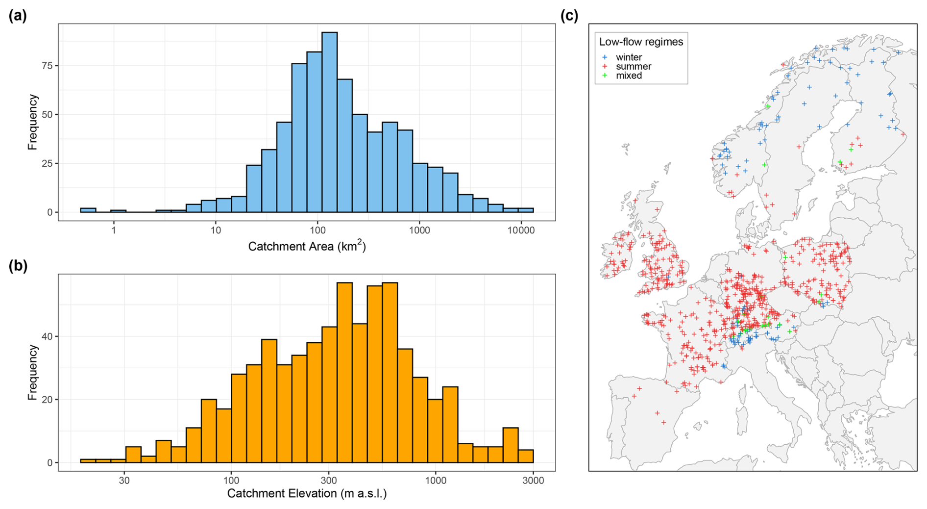
Figure 1 Catchment characteristics and low-flow regime classification for the study area. (a)–(b) show the distributions of catchment area and mean elevation (both on logarithmic scales). (c) show the spatial distribution of low-flow regimes derived using PAM clustering, distinguishing winter-dominated, summer-dominated, and mixed regimes.

3 Methods

This section presents the framework of NSLFA_mixC developed in this study (Fig. 2). The workflow consists of (i) data pre-processing and seasonal stratification, (ii) testing for non-stationarity and inter-seasonal dependence, (iii) model selection based on likelihood-based criteria (iv) estimation of stationary and non-stationary marginal low-flow distributions, (v) estimation of stationary and non-stationary mixed distribution and mixed copula models, and (vi) model performance evaluation using gain metrics.

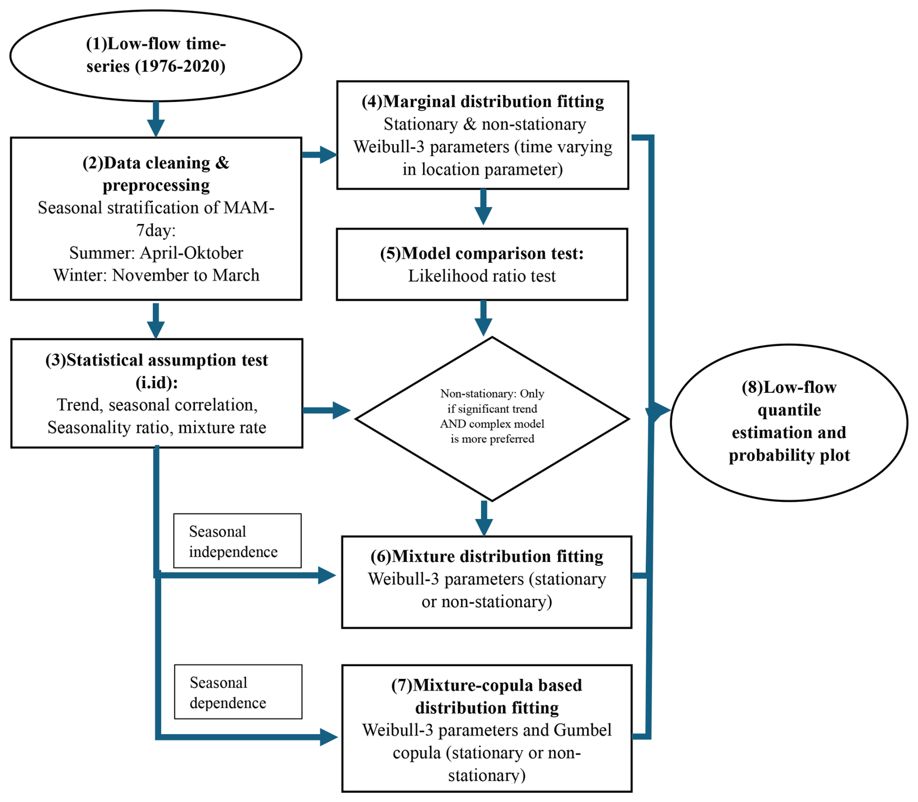
Figure 2 Workflow of the NSLFA framework. The procedure includes data pre-processing and seasonal stratification, testing of statistical assumptions, fitting and comparing stationary and non-stationary marginal Weibull distributions, modelling seasonal dependence using either a mixed distribution or a mixed distribution-copula approach, and estimation of low-flow quantiles and probability plots.

3.1 Data pre-processing

3.1.1 Delineation of homogeneous regions using partitioning around medoids (PAM)

To support a hydrologically meaningful regional interpretation of seasonal low-flow regimes, homogeneous low-flow regimes were delineated using seasonality histograms (SH) and classified using partitive clustering based on the partitioning around medoids (PAM), which helps identify dominant hydrological controls, reduce heterogeneity, and improve model choice (Laaha and Blöschl, 2006; Kaufman and Rousseeuw, 2009). SH describe the seasonal distribution of low flows using 12 variables that represent monthly frequencies of low flows. Low-flow days were identified from the M7Q series, obtained by smoothing the daily discharge series with a 7 d moving average, using a catchment-specific threshold Q₉₅, corresponding to the discharge exceeded on 95 % of days, which is a commonly used threshold in low-flow studies. A low-flow day is when its M7Q value is below Q₉₅ (Laaha and Blöschl, 2006).

For each catchment, monthly occurrence frequencies were calculated as the ratio of low-flow days to total observations in each calendar month, yielding a 12-dimensional SH vector that captures the timing and shape of low-flow seasonality. These SH vectors were then grouped using PAM clustering (Kaufman and Rousseeuw, 2009; Laaha, 2002) with the number of clusters selected from the silhouette plot, which orders the silhouette width of each SH and reflects its similarity to the assigned cluster relative to the nearest alternative cluster. PAM clustering of seasonality histograms identifies whether low-flow events occur predominantly in summer, winter or both seasons, thereby providing regional evidence that annual low-flow minima may originate from different seasonal generating processes and supporting the need for a seasonal mixture framework. Clusters were interpreted based on the seasonal peaks of their medoid histograms to identify dominant seasonal low-flow regimes, whereas catchments with silhouette widths below 0.2 were considered to have weak cluster membership and were therefore classified as having mixed seasonality (Laaha and Blöschl, 2006; Laaha, 2003).

3.1.2 Seasonal stratification

The annual low-flow series (AM) consists of the minimum 7 d average streamflow observed in each hydrological year (April to March), obtained from the M7Q series. The moving average filter reduces short-term variability and is widely applied in low-flow studies (Laaha et al., 2017; Floriancic et al., 2021). Let $X_{\mathrm{1}},\mathrm{\dots },X_n$ denote a sequence of independent and identically distributed (i.i.d.) random variables with common distribution function F (Coles et al., 2001). Under the conventional annual-minima approach, the annual low-flow series is defined as:

$$\begin{array}{}\text{(1)}& \mathrm{AM}=min\mathit{\{}{X}_{\mathrm{1}},\mathrm{\dots },X_n\mathit{\}}.\end{array}$$

which implicitly assumes that annual low flows are generated by a homogeneous underlying process. However, in seasonal climates, low-flow events may arise from distinct hydrological processes operating in different seasons (Laaha and Blöschl, 2007; Tallaksen and Van Lanen, 2023). In such cases, the annual minimum can be expressed as the minimum of the annual summer minima (AM_S) and winter minima (AM_W) (Laaha, 2023b),

$$\begin{array}{}\text{(2)}& \mathrm{AM}=min\mathit{\{}{\mathrm{AM}}_{\mathrm{S}},{\mathrm{AM}}_{\mathrm{W}}\mathit{\}}.\end{array}$$

For each catchment, the dependence between the annual summer and winter low-flow series was assessed using Kendall's rank correlation coefficient (τ) (Kendall, 1976). Statistical significance was evaluated at the 5 % level, and correlations with p>0.05 were classified as non-significant. Only significant correlations were subsequently grouped, for interpretation purposes, into weak ($\mathrm{0.10}\le \mathit{\tau }<\mathrm{0.30}$), moderate ($\mathrm{0.30}\le \mathit{\tau }<\mathrm{0.55}$), and strong (τ≥0.55) dependence classes. In addition, a mixture rate was calculated as the proportion of years in which the summer minimum 7 d flow was lower than the winter minimum 7 d flow. Based on this rate, catchments were classified as summer-dominated (>0.55), winter-dominated (<0.45), or mixed (0.45–0.55). This provides a gradual measure of seasonal dominance at the individual-catchment scale, whereas PAM clustering yields a discrete classification into mutually exclusive regime groups (Laaha and Blöschl, 2006).

3.1.3 Trend analysis

In this study, non-stationarity is assessed by separately detecting trends in the summer (AM_S) and winter (AM_W) low-flow series using the non-parametric modified Mann-Kendall test with block bootstrapping (BBSMK) with block size determined from the number of contiguous significant serial correlations, plus an additional η=1 (Patakamuri et al., 2020). Compared to the original Mann-Kendall test, BBSMK preserves the original data structure, accounts for autocorrelation in the time series, and reduces the risk of false trend detection. Due to its resampling technique, the method is robust even for relatively short records (Önöz and Bayazit, 2012; Patakamuri et al., 2020). A total of 2000 bootstrap replicates is generated to construct the empirical distribution of the Mann-Kendall test statistic. Statistical significance is evaluated using the empirical bootstrap confidence interval of the standardised test statistic (Z). A trend is considered significant at the 95 % confidence level when the observed Z value lies outside the corresponding 95 % empirical bootstrap confidence interval. The magnitude of the trend is quantified using the Sen slope estimator, a robust non-parametric estimate of the monotonic rate of change based on the median of all pairwise slopes. Positive and negative values indicate increasing and decreasing trends, respectively (Sen, 1968).

3.2 NSLFA_mixC framework for low flows

3.2.1 Stationary mixed copula approach for low flows

The AM_S and AM_W are samples from two random variables S (annual summer low flow) and W (annual winter low flow). Under the assumption that summer and winter events are independent, the probability that the low-flow event is equal to or smaller than magnitude q can be obtained from its seasonal non-exceedance probabilities:

$$\begin{array}{}\text{(3)}& F_{\mathrm{S}}\left(q\right)=P(S\le q),F_{\mathrm{W}}\left(q\right)=P(W\le q),\end{array}$$

Given that the same discharge magnitude q is inserted into both marginal distributions, the mixed probability estimator can be written as

$$\begin{array}{}\text{(4)}& F_{\mathrm{mix}}\left(q\right)=\mathrm{1}-(\mathrm{1}-F_{\mathrm{S}}(q\left)\right)(\mathrm{1}-F_{\mathrm{W}}(q\left)\right).\end{array}$$

This estimator provides a valid generalisation of the annual-frequency estimator and yields improved probability estimates when the summer and winter distributions differ (Laaha, 2023a). Following the Fisher–Tippett–Gnedenko theorem, seasonal low-flow minima are modelled using three-parameter Weibull (WEI3) distributions for both summer and winter,

$$\begin{array}{}\text{(5)}& F_i\left(q\right)=\mathrm{1}-\exp \left[-{\left({\displaystyle \frac{q-{\mathit{\mu }}_i}{{\mathit{\sigma }}_i}}\right)}^{{\mathit{\xi }}_i}\right],i\in \mathit{\{}S,W\mathit{\}},\end{array}$$

defined for q>μ_i, where μ_i denotes the location parameter, σ_i>0 the scale parameter, and ξ_i>0 the shape parameter of the WEI3 distribution. The parameters are estimated separately for each season by maximum likelihood (ML) which is adopted for its flexibility in accommodating changes in model structure, which is important for extending from stationary to non-stationary settings (Coles et al., 2001).

The multiplication rule assumes that the events in the two seasons are independent. However, this is not always the case, leading to a more general bivariate frequency problem in which the joint occurrence probability of events in two variables is required. This can be addressed using bivariate frequency analysis, in which a joint probability model is used to estimate the probability that both S and W do not exceed given magnitudes s and w,

$$\begin{array}{}\text{(6)}& P(S\le s,W\le w)=F_{\mathrm{S},\mathrm{W}}(s,w).\end{array}$$

To model the joint distribution $F_{\mathrm{S},\mathrm{W}}(s,w)$, a copula-based approach is applied. A copula is a function that fully characterises the dependence structure between random variables independently of their marginal distributions (Sklar, 1959; Klein et al., 2010). Following Sklar’s theorem, the joint cumulative distribution function can be written as

$$\begin{array}{}\text{(7)}& F_{\mathrm{S},\mathrm{W}}(s,w)=C\left(F_{\mathrm{S}}\left(s\right),F_{\mathrm{W}}\left(w\right)\right),\end{array}$$

where C(⋅) denotes a bivariate copula.

In this study, the Gumbel-Hougaard copula was chosen, motivated by the pan-European comparative assessment of copula-based mixed estimators presented by Laaha (2023b). Although alternative families (e.g. Frank and Plackett) performed well for individual catchments, the Gumbel copula emerged as a robust and station-wide suitable model for capturing positive tail dependence in seasonal low-flow extremes and was therefore adopted for continental-scale applications (Laaha, 2023b). Following this established evidence, and given that the focus of the present study is on extending the mixed copula framework to non-stationary conditions, alternative copula families are not re-evaluated here. The Gumbel copula is defined as

$$\begin{array}{}\text{(8)}& \begin{array}{rl}{C}_{\mathit{\theta }}(u,v)=& \exp \left(-{\left[(-\ln u{)}^{\mathit{\theta }}+(-\ln v{)}^{\mathit{\theta }}\right]}^{\mathrm{1}/\mathit{\theta }}\right),\\ & \mathit{\theta }\in [\mathrm{1},\mathrm{\infty }),\end{array}\end{array}$$

where u and v denote the pseudo-observations corresponding to the marginal probabilities of S and W, respectively. The parameter θ is directly related to Kendall’s rank correlation coefficient τ.

The copula-based mixed probability estimator for annual low-flow occurrences is obtained by inserting the same discharge magnitude q into both marginal distributions and applying the AND-operator for minima. This yields

$$\begin{array}{}\text{(9)}& F_{\mathrm{mix},C}\left(q\right)=F_{\mathrm{S}}\left(q\right)+F_{\mathrm{W}}\left(q\right)-C_{\mathit{\theta }}\left(F_{\mathrm{S}}\left(q\right),F_{\mathrm{W}}\left(q\right)\right).\end{array}$$

For the special case of independence (θ=1), the copula reduces to the independence copula and $C\left(F_{\mathrm{S}}\left(q\right),F_{\mathrm{W}}\left(q\right)\right)=F_{\mathrm{S}}\left(q\right)F_{\mathrm{W}}\left(q\right)$, such that Eq. (9) simplifies to the mixed distribution estimator in Eq. (4). The mixed copula estimator therefore represents a valid generalisation of the mixed distribution approach for situations where summer and winter low flows are not independent (Laaha, 2023b).

3.2.2 Non-stationary mixed copula approach for low flows

Under non-stationary conditions, both seasonal low-flow behaviour and the dependence between summer and winter low flows may change over time. To account for such changes, the mixed copula framework is extended to allow temporal variation in both the marginal distributions and the dependence structure.

Non-stationarity in seasonal low-flow behaviour is represented by allowing the location parameter of the marginal Weibull distributions to vary linearly with time, while keeping the scale and shape parameters constant. Allowing additional parameters to vary without strong empirical support substantially increases estimation uncertainty. Moreover, scaling analysis indicates that the moments of streamflow series (mean, variance, and skewness) are nearly perfectly related (Vogel and Sankarasubramanian, 2000), suggesting that independent temporal variation in scale and shape parameters would be inconsistent with these structural dependencies (Serago and Vogel, 2018). Let $t=\mathrm{1},\mathrm{\dots },n$ denote the (annual) time index of the observation record. The time-dependent location parameter is then defined as

$$\begin{array}{}\text{(10)}& \mathit{\mu }\left(t\right)={\mathit{\beta }}_{\mathrm{0}}+{\mathit{\beta }}_{\mathrm{1}}t,\end{array}$$

where β₁ quantifies the temporal trend in low-flow magnitude. Accordingly, the seasonal marginal distributions are expressed as time-dependent cumulative distribution functions,

$$\begin{array}{}\text{(11)}& F_{\mathrm{S}}(q\mid t)=P(S\le q\mid t),F_{\mathrm{W}}(q\mid t)=P(W\le q\mid t),\end{array}$$

with non-stationarity in both summer and winter low-flow series introduced through the time-varying location parameter of the WEI3 distribution. Assuming seasonal independence, the non-stationary mixed distribution for annual low flows is obtained by inserting F_S(q∣t) and F_W(q∣t) into Eq. (4).

To explicitly account for inter-seasonal dependence that may itself vary over time, a non-stationary copula-based estimator is adopted. As in the stationary case, a Gumbel-Hougaard copula is used to model positive dependence between seasonal low flows, but now with a time-variant parameter θ. The non-stationary copula is defined as

$$\begin{array}{}\text{(12)}& \begin{array}{rl}{C}_{\mathit{\theta }\left(\mathrm{t}\right)}(u,v)=& \exp \left(-{\left[(-\ln u{)}^{\mathit{\theta }\left(\mathrm{t}\right)}+(-\ln v{)}^{\mathit{\theta }\left(\mathrm{t}\right)}\right]}^{\mathrm{1}/\mathit{\theta }\left(\mathrm{t}\right)}\right),\\ & \mathit{\theta }\left(t\right)\in [\mathrm{1},\mathrm{\infty }),\end{array}\end{array}$$

where $u=F_{\mathrm{S}}(q\mid t)$ and $v=F_{\mathrm{W}}(q\mid t)$ denote time-dependent pseudo-observations and

$$\begin{array}{}\text{(13)}& \mathit{\theta }\left(t\right)=\mathrm{1}+\exp \left({\mathit{\gamma }}_{\mathrm{0}}+{\mathit{\gamma }}_{\mathrm{1}}{z}_{\mathrm{t}}\right),\end{array}$$

where $z_{\mathrm{t}}\in [\mathrm{0},\mathrm{1}]$ is a standardized time covariate. This formulation ensures valid parameter values and allows for gradual changes in dependence strength over time, and assuming the observations are independent, the likelihood functions for the stationary and non-stationary WEI3 models are provided in Appendix A.

The non-stationary copula-based mixed probability estimator for annual low-flow occurrences is then obtained analogously to Eq. (9). The non-stationary mixed copula estimator therefore represents a generalisation of both the stationary mixed copula approach and the non-stationary mixed distribution approach, allowing simultaneous representation of temporal changes in marginal low-flow behaviour and inter-seasonal dependence.

Design low-flow quantiles for a given return period T are finally obtained by numerical inversion of the time-dependent form of Eq. (9) at selected time points, yielding time-dependent return levels that reflect evolving seasonal processes and dependence structures.

3.3 Model comparison

Model selection using likelihood ratio test

Stationary and non-stationary marginal models are compared using the likelihood ratio (LR) test within a nested modelling framework, where M1 denotes the simpler stationary model and M2 the more complex non-stationary model (Coles et al., 2001). The LR deviance statistic is defined as

$$\begin{array}{}\text{(14)}& D=\mathrm{2}\left\{\mathrm{\ell }\left(\mathrm{M}\mathrm{2}\right)-\mathrm{\ell }\left(\mathrm{M}\mathrm{1}\right)\right\},\end{array}$$

where ℓ(M1) and ℓ(M2) denote the maximized log-likelihoods of the stationary and non-stationary models, respectively.

Model selection follows a parsimony principle, whereby a non-stationary model is adopted only when the LR test indicates a statistically significant improvement over the stationary formulation.

3.4 Model evaluation methods

Model evaluation follows the gain-based framework of Laaha (2023a, b), in which deviations between alternative estimators are interpreted as relative gains or losses in accuracy rather than absolute errors. This interpretation reflects the fact that the true low-flow distribution is unknown and that models incorporating additional hydrological process information are considered conceptually superior to simpler representations. It should be noted that the interpretation of the deviation as a gain depends on the assumption that the model provides a more appropriate representation of the underlying low-flow process than the alternative model. The terminology is therefore used in the context of nested model comparisons, where the more complex formulation extends the simpler alternative. The evaluation is based on the differences in the estimated return periods for selected design events. As low flows represent minima, return periods are defined as the reciprocal of the non-exceedence probability, $T=\mathrm{1}/p$.

In the stationary framework, model performance is evaluated by comparing return period estimates from one conventional model M1 with those from an extended model M2, e.g. the mixture model or mixture copula model. For a given return period T_M1, the corresponding annual low-flow quantile is first estimated from the conventional model M1 and then inserted into the alternative probability models M2 to obtain the associated return periods T_M2.

The performance gain of the extended estimators relative to the conventional estimator is quantified using the relative deviation

$$\begin{array}{}\text{(15)}& {\mathrm{rd}}_{\mathrm{T}}={\displaystyle \frac{T_{\mathrm{M}\mathrm{1}}-T_{\mathrm{M}\mathrm{2}}}{T_{\mathrm{M}\mathrm{2}}}},\end{array}$$

Positive values indicate that the conventional estimator overestimates the return period relative to the extended estimator. To avoid cancellation when aggregating results, the relative absolute deviation ${\mathrm{rad}}_{\mathrm{T}}=\left|{\mathrm{rd}}_{\mathrm{T}}\right|$ is also reported. The added value of explicitly accounting for seasonal dependence is assessed by comparing the mixed distribution (M1 =mix) and mixed copula estimators (M2 =mixC).

In the non-stationary framework, the same evaluation principle is applied, but return periods are evaluated at selected temporal snapshots t. When rdT is used to compare two different time points within the non-stationary model, it should be interpreted as a distributional shift, expressed as a change in estimated return period, rather than as a performance gain. For either non-stationary approach, let T(t) denote the time-dependent return period at snapshot t, i.e., $T\left(t\right)\in \mathit{\left\{}{T}_{\mathrm{ns}.\mathrm{mix}}\right(t),T_{\mathrm{ns}.\mathrm{mixC}}(t\left)\mathit{\right\}}$. Changes in low-flow severity between two snapshots, t₁ and t₂, are quantified as well as the difference between a stationary model and a non-stationary model with parameters at the end of the observation period.

Corresponding relative absolute deviations are additionally reported for aggregation. Together, these metrics quantify the added value of accounting for seasonal heterogeneity, seasonal dependence, and temporal non-stationarity in low-flow frequency analysis.

4 Results and Discussion

4.1 Seasonal regimes, dependence, and trends

The classification of seasonality histograms with PAM clustering shows pronounced spatial low-flow regimes across Europe (Fig. 1c). Three regimes are identified: summer, winter, and mixed seasonality. Summer regimes dominate, comprising 82.5 % of the catchments, and are distributed mainly across western, central, and southern Europe. Their seasonal peaks between April and October indicate low-flow conditions primarily associated with warm-season precipitation deficits and high evaporative demand. This broad pattern is also in line with recent studies pointing to a contribution of internal multidecadal North Atlantic Variability to the warming of early spring droughts in Europe (Haslinger and Mayer, 2023). Winter regimes account for 14.4 % of the catchments and occur mainly in northern Europe and mountainous regions, where peaks between November and March reflect the influence of snow accumulation and other cold-season hydrological processes. The remaining 3.1 % of catchments, classified as mixed seasonality based on silhouette widths below 0.2, indicating weak or less distinct seasonal dominance (Sect.3.1.1). The classification is robust to the choice of silhouette-width threshold, with thresholds of 0.15 and 0.25 retaining 98.47 % and 98.89 % agreement, respectively, with the baseline threshold of 0.2, changes primarily affect the proportion of catchments classified as mixed. Additional sensitivity analyses of the clustering approach and seasonal definition similarly support the robustness of the dominant summer-winter structure, with detailed results provided in Appendix B. This result is consistent with the mixture-rate analysis results shown in the Appendix C, which likewise highlights the predominance of summer low-flow conditions across the study domain.

Trend patterns also differ between the summer and winter low flow series. Figure 3a–b show that significant trends are more common in summer than in winter, occurring in 36.1 % and 18.1 % of catchments, respectively, while non-significant trends dominate overall, particularly in winter (82.1 %). This suggests a greater sensitivity of summer low flows to long-term hydrological change. In summer, decreasing trends dominate (73.8 % of significant cases) and are concentrated mainly in western, central, and southern Europe. In winter, decreasing trends are more frequent than increasing trends (59.2 %), but the share of increasing trends (40.8 %) is notably higher than in summer, particularly in northern Europe and snow-influenced regions. These patterns suggest that summer low flows are shaped by the combined effects of warming, enhanced evapotranspiration, drought intensification, and regional precipitation deficits, particularly in central Europe (Zeder and Fischer, 2020), whereas winter low flows reflect a more mixed response linked to snow processes and cold-season hydrological dynamics.

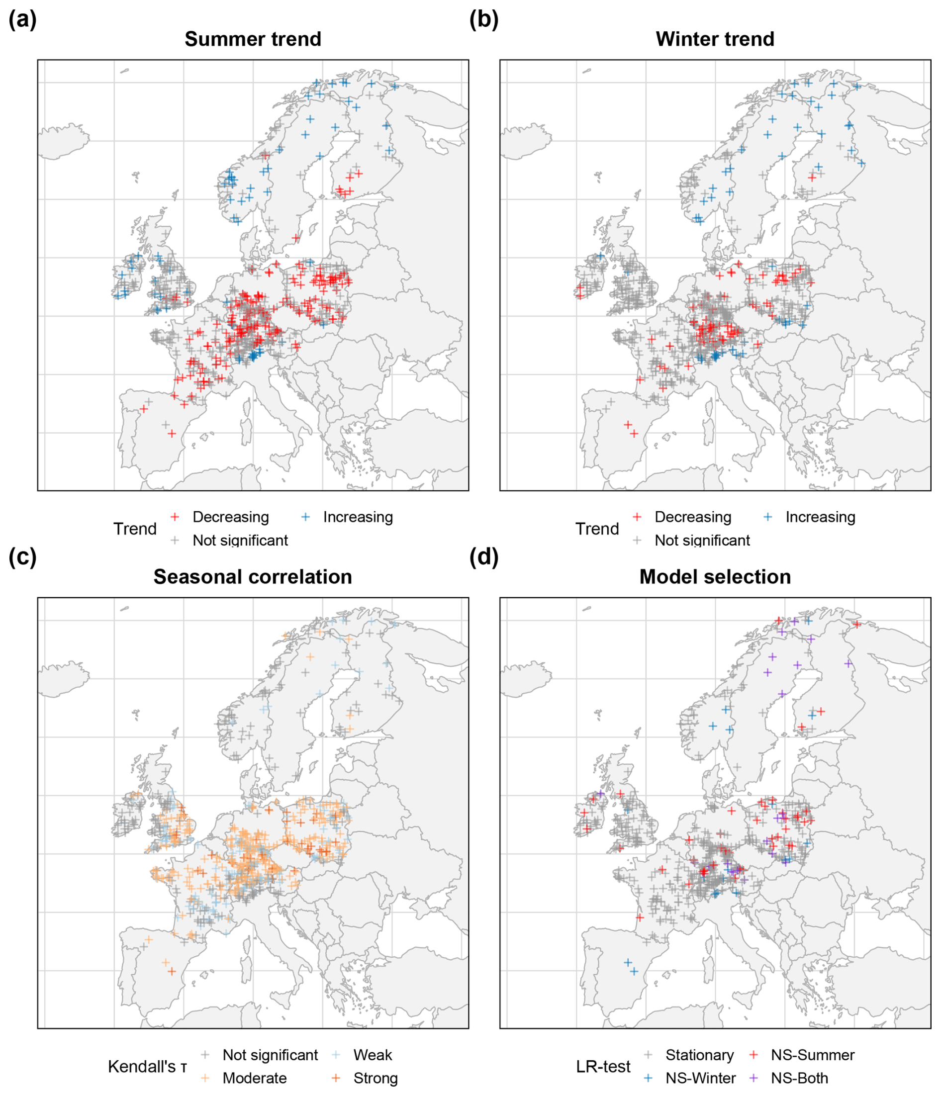
Figure 3 Spatial distribution of statistical assumption tests and final model selection. (a)–(b) show significant and non-significant trends in summer and winter low-flow series across the study catchments, based on the block bootstrap Mann-Kendall test. (c) summarises dependence between seasonal low-flow using Kendall's τ, while (d), shows the final model decision, distinguishing stationary catchments from those requiring non-stationary modelling in summer, winter, or both seasons.

The dependence analysis further shows that summer and winter low flows are neither fully independent nor strongly coupled across most catchments. Using the significance criterion and Kendall's τ classes defined in Sect. 3.1.2, significantly low to moderate Kendall's τ correlations dominate the study domain (Fig. 3c), accounting for 41.5 % and 25.9 % of catchments, respectively, whereas strong significant correlations are rare (0.1 %). Non-significant correlations are primarily confined to the low-correlation class (32.3 %), indicating that seasonal dependence is common but generally weak to moderate, implying that the two seasonal components often share part of the same hydro-climatic forcing while still retaining distinct behaviour.

Taken together, these results show that low-flow regimes across the study area are governed by different generating processes, varying degrees of seasonal dependence, and temporal dynamics, thereby highlighting the need for a low-flow frequency analysis framework that is flexible but also explicitly accounts for these conditions.

4.2 Application and evaluation of the NSLFA_mixC framework

4.2.1 Model selection and spatial distribution of non-stationarity

The first step in applying the NSLFA_mixC framework is to fit the WEI3 distribution to the low-flow time series. The use of the WEI3 distribution is theoretically motivated by the Fisher-Tippett-Gnedenko theorem, as the Weibull distribution represents a limiting distribution for lower extremes with a finite lower bound and is therefore well established in low-flow frequency analysis. Nevertheless, departures from the fitted distribution may occur at individual catchments. Such departures are interpreted not only as a distributional issue, but also as a diagnostic indication of sample properties, particularly process heterogeneity between summer and winter low-flow generation. Alternative low-flow distributions may also provide suitable representations at individual catchments. However, the present study retains WEI3 because of its theoretical basis for lower extremes and its consistency with the established LFA_mixC framework.

In this study, WEI3 with ML estimation converged to feasible parameter estimates in 76.1 % of catchments, indicating that the procedure is suitable for modelling low-flow behaviour in most cases. The remaining optimisation failures are likely related to the constrained parameter space, which may yield infeasible parameter combinations. The unsuccessful fits were distributed throughout the study domain rather than being concentrated in a single geographical region, while the successfully fitted catchments retained broad spatial coverage across Europe. Unsuccessfully fitted catchments tended to be smaller and generally had lower low-flow values relative to catchment area in the annual, summer, and winter series, with less year-to-year variability. Mean catchment elevation was similar between the two groups. The unsuccessful catchments also showed consistently higher positive L-skewness, indicating differences in the distributional shape of their low-flow series. These characteristics may contribute to the greater difficulty in estimating the WEI3 parameters within the constrained parameter space. Similar convergence issues have been reported in earlier low-flow studies (Vogel and Kroll, 1989), suggesting that they arise from the estimation procedure rather than a general limitation of the WEI3 distribution itself. We also provide the corresponding spatial comparison and detailed catchment, low-flow, and distributional characteristics in Appendix D.

After fitting the stationary and non-stationary WEI3 distributions to annual and seasonal low-flow data, the evidence supporting the more complex non-stationary formulation must be evaluated for each catchment to avoid overfitting and increased estimation bias. Based on the likelihood ratio test with 5 % significance level, comparing stationary and non-stationary WEI3 models, 84.5 % of summer catchments and 91.3 % of winter catchments favour the simpler stationary model, whereas 15.5 % and 8.7 %, respectively, show a statistically significant improvement when non-stationarity is introduced.

When combining the results of the likelihood ratio test and the Mann-Kendall trend test, the proportion of catchments classified as non-stationary in both cases decreases slightly to 12.2 % in summer and 7.7 % in winter, while the stationary model remains preferred in 87.8 % and 92.3 % of catchments, respectively. The reduction is expected, as the combined criterion is more restrictive and requires both improved statistical fit and evidence of temporal change. In addition, the Type-I error of statistical tests has to be considered. The results indicate that stationary formulations remain adequate for most catchments, while a non-negligible subset exhibits evidence of temporal change that cannot be ignored and justifies the more complex non-stationary representation, with a clearer signal in summer than in winter, which is consistent with the trend analysis presented in Sect. 4.1.

The spatial distribution of the model selection (Fig. 3d) further shows that non-stationarity is spatially structured rather than randomly distributed across the study domain. Catchments classified as non-stationary in summer-only are more frequent and occur mainly in central and eastern Europe, whereas winter-only non-stationary catchments are less common and more scattered. Catchments requiring non-stationary modelling in both seasons are concentrated particularly in northern Europe and other snow-influenced regions, suggesting that temporal change there affects both seasonal components simultaneously. By contrast, stationary models dominate across much of western and central Europe, indicating that for most catchments the simpler stationary model remains sufficient.

The observed spatial structure therefore suggests that the detected non-stationarity may be linked to differences in low- flow generating processes across regions and catchment types. Although the ROBIN Level-1 network minimises direct human influence, low-flow regimes are strongly controlled by catchment storage and release processes, including soil and aquifer characteristics, recharge, evapotranspiration, vegetation, topography, and climate (Smakhtin, 2001). Therefore, residual effects from small abstractions, groundwater interactions, land- use change, local water management, reservoirs, or flow regulation cannot be fully excluded and may contribute to temporal changes in some catchments.

Overall, these results suggest that the proposed non-stationary framework is particularly relevant for catchments with evident non-stationarity, even though it is not required for all catchments. Its value lies not in universally replacing stationary models, but in identifying and representing catchments where seasonal low-flow regimes exhibit temporal change. In this case, the stationarity assumption may be violated and should not be ignored in the frequency analysis. To keep the framework parsimonious, non-stationarity was introduced as a linear trend in the location parameter and was evaluated formally by comparing the non-stationary and stationary models using a likelihood-ratio test. The linear formulation was chosen as a simple and parsimonious way to represent gradual temporal change. Given the limited record length, more flexible non-linear formulations or time-varying scale and shape parameters would require stronger empirical support and could substantially increase estimation uncertainty and the risk of overfitting. More complex temporal dynamics, including regime shifts, accelerations, thresholds, or oscillatory behaviour linked to climatic variability, may also occur. Nonlinear formulations, change-point approaches, or climatic covariates could therefore be considered where sufficiently long records and supporting evidence are available. Therefore, NSLFA_mixC provides an extension of the stationary framework, preserving its conceptual basis while improving the representation of evolving low-flow conditions where non-stationarity is evident. Given that the stationary model remains a special case of the more complex non-stationary model, the non-stationary model provides a robust framework that can cover both sides.

Finally, intermittent-flow conditions relevant to the applicability of the WEI3-based framework were identified by comparing the ROBIN catchments used in this study with the intermittent-flow classifications of Tramblay et al. (2021). There are 3.2 % of catchments that were classified as intermittent and were retained in the analysis. Because the WEI3 distribution is continuous and cannot explicitly represent a probability mass at zero, catchments with repeated zero-flow occurrences would require a modelling framework that accounts for zero flows, for example by treating zeros as censored observations within a mixed discrete-continuous L-moment framework (Laaha, 2023a, b; Bhatti et al., 2019). However, explicitly accounting for these data conditions is beyond the scope of the current study..

4.2.2 Catchment-scale application: illustrative case study

To illustrate the practical application of the NSLFA_mixC framework, the catchment Stauf Vöckla at Traun in Upper Austria is used as a representative example. The catchment covers an area of 99.7 km² and has a mean elevation of 503 m a.s.l. Figure 4a shows the time series of observed summer and winter minimum flow. Trend analysis using BBMSK identified a significant decreasing trend in summer flow, whereas no significant trend was detected in winter. The catchment is further characterised by moderate seasonal dependence (Kendall's τ=0.48) and a nearly balanced mixture rate (0.52), indicating a mixed seasonal low-flow regime. Stationary and non-stationary WEI3 distributions were then fitted separately to the annual series, used here as a reference model, and to the seasonal series. Based on the likelihood ratio and trend test, the non-stationary model was preferred for summer, whereas the stationary model was not rejected for winter. Notably, this seasonal contrast is already visible in Fig. 4a, where temporal change is more evident in summer than in winter.

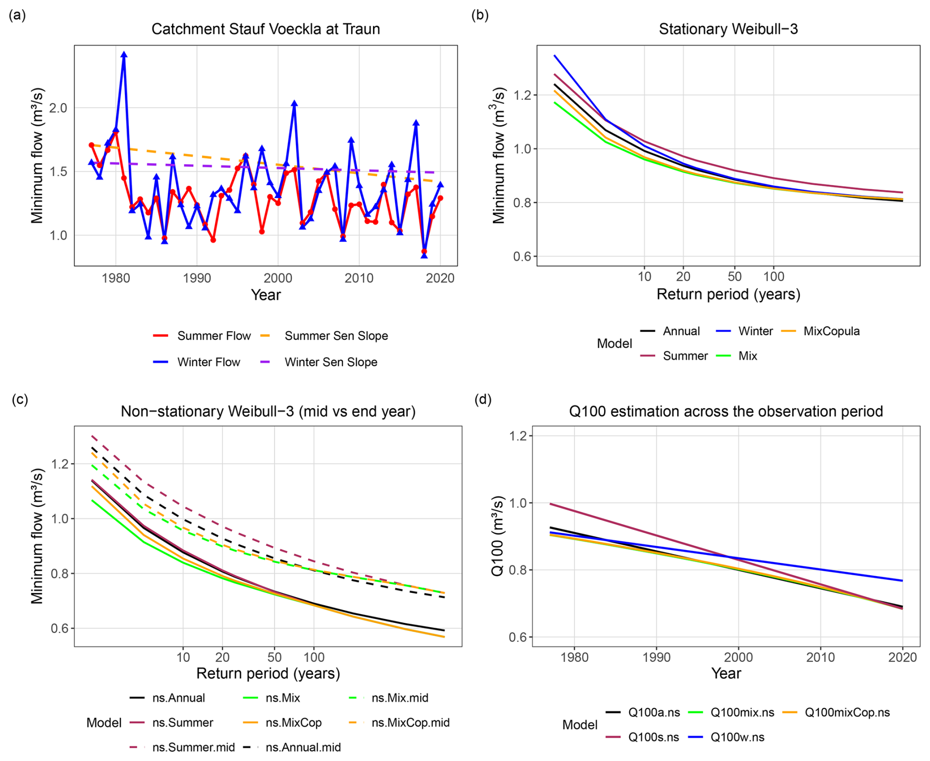
Figure 4 Catchment Stauf Vöckla at Traun (a) Observed summer and winter minimum 7 d flows (M7Q) with corresponding Sen’s slope trend estimates. (b) Stationary WEI3 return period curves for summer, winter, annual, and seasonal mixture (independence and Gumbel copula) models. (c) Non-stationary WEI3 return level curves evaluated at the mid-point and final year of the record, including NS mixture and NS copula-mixture formulations. (d) Temporal evolution of the 100-year low-flow quantile (Q₁₀₀) under non-stationary seasonal, annual, mixture, and mixture-copula models, illustrating how changes in seasonal regimes propagate into extreme low-flow behaviour.

Under stationary conditions, five low-flow frequency models were fitted using WEI3 distribution and Gumbel-Hougaard copula following the framework of Laaha (2023a, b): the annual, summer, winter, mixture, and mixture-copula models. Figure 4b shows the resulting stationary probability plot across different return periods (T). The practical interpretation focuses mainly on the 100-year return period, which can be used as a stress-test or worst-case scenario in water management and infrastructure planning (Hodgkins et al., 2024). In this study, the 100-year return period is used to compare the sensitivity of low-flow estimates to seasonality, dependence, and non-stationarity, while higher return periods are shown only for illustrative comparison of lower-tail behaviour.

For all models, estimated minimum flows decrease with increasing return period. Importantly, the annual curve lies above the mixture-based estimators, indicating that explicit representation of seasonal structure yields lower, and therefore more extreme, design low-flow estimates. The mixture and mixture-copula curves are very close, consistent with the catchment's moderate inter-seasonal dependence. Their differences are more visible at short return periods (T<10 years), which are less relevant for design purposes. In this respect, this behaviour is consistent with Laaha (2023a, b) showing that under moderate seasonal dependence, the copula-based correction has only a limited influence, whereas larger differences would be expected for increased seasonal dependence between summer and winter low-flow components.

When non-stationarity is explicitly taken into account, the seasonal WEI3 location parameter is allowed to vary over time, while the scale and shape parameters are kept constant. For the copula-based formulation, the dependence parameter is also time-varying (Sect.3.2.2). The effect of this formulation is illustrated by the non-stationary probability plot in Fig. 4c. Because non-stationarity was detected in summer, but not in winter, the non-stationarity comparison is shown only for the annual, summer, mixture, and mixture-copula models. The probabilities are evaluated at two reference points: the midpoint in 1998 (dashed lines) and the end of the observation period in 2020 (solid lines) to capture more recent conditions. The separation between the dashed and solid lines indicates a downward shift in estimated low-flow magnitudes over time across all models. Notably, summer low flows were lower in 2020 than in 1998, confirming a shift in the summer low flow regime. At the same time, the mixture-copula model accounting for time-varying dependence yields similar behaviour to the stationary models, where the difference between the mixture and the copula-based mixture remains small. Overall, this Fig. 4c indicates that the temporal behaviour of the low-flow regime cannot be fully described under a stationary assumption.

This temporal change becomes even clearer when examining the evolution of extreme low-flow Q₁₀₀ over the full observation period. Figure 4d shows that all non-stationary Q₁₀₀ estimates decline over time, indicating a general intensification of low-flow conditions. At the beginning of the record, the summer curve lies above the winter curve, implying that winter low flows are initially more severe than summer low flows. Over time, however, the two seasonal curves then converge around the middle of the period, and towards the end of the period, the summer curve falls below the winter curve. This clearly shows a gradual shift from winter dominance to summer dominance. The annual, mixture, and mixture-copula estimates closely track this transition and remain very similar throughout, suggesting that for this catchment the effect of seasonal dependence on the long-term evolution of Q₁₀₀ is relatively small compared with the overall temporal decline. Comparing return periods from the NSLFA_mixC (Sect. 3.4) between the start of the observation period in 1976 and its end in 2020 suggests a substantial increase in the frequency of extreme low flows within the observed record. In particular, an event corresponding to a 100-year return period in 1976 is associated with a return period of about 43 years by 2020, indicating that such an event became approximately on average 2.3 times as frequent according to the fitted non-stationary model. This comparison is a statistical diagnostic of change within the historical observation period and should not be interpreted as a projection of future event frequency.

To further illustrate the framework under contrasting hydro-climatic conditions, we analysed the catchment Oksfjordvatn in Norway as a second example. Unlike Stauf Vöckla, which represents a mixed seasonal regime (mixture rate = 0.52), Oksfjordvatn is winter-dominated (mixture rate = 0.40) and exhibits weaker inter-seasonal dependence (Kendall's τ=0.26, compared with 0.48 at Stauf Vöckla). The temporal behaviour also differs between the two catchments. At Stauf Vöckla, non-stationarity is mainly associated with declining summer low flows, whereas at Oksfjordvatn both summer and winter components were identified as non-stationary and low-flow magnitudes increase over time. Consequently, the non-stationary Q₁₀₀ estimates decrease through time at Stauf Vöckla, indicating increasingly severe low-flow conditions, but increase at Oksfjordvatn, indicating less severe low-flow conditions toward the end of the observation period. The corresponding four-panel analysis for Oksfjordvatn is provided in Appendix E.

Overall, both examples demonstrate how the NSLFA_mixC framework captures seasonal contrasts, temporal shifts, and dependence effects within a single coherent analysis. It also illustrates that non-stationarity may alter not only the magnitude of design low flows, but also the relative importance of summer and winter contributions to the annual low-flow regime.

4.3 Performance evaluation and model gains

In the following, we assess the performance of the full non-stationary framework across European catchments. A benchmark comparison of the stationary annual and stationary mixture-based estimators is provided in Appendix F. As the main focus here is the extension to non-stationary low-flow frequency analysis, the detailed stationary benchmark is not discussed further in the main text.

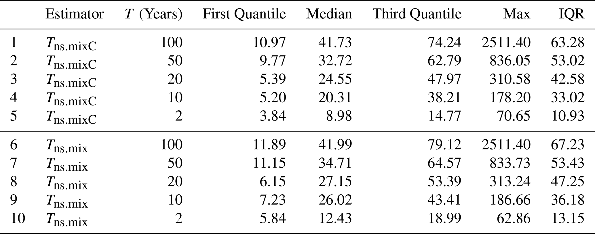
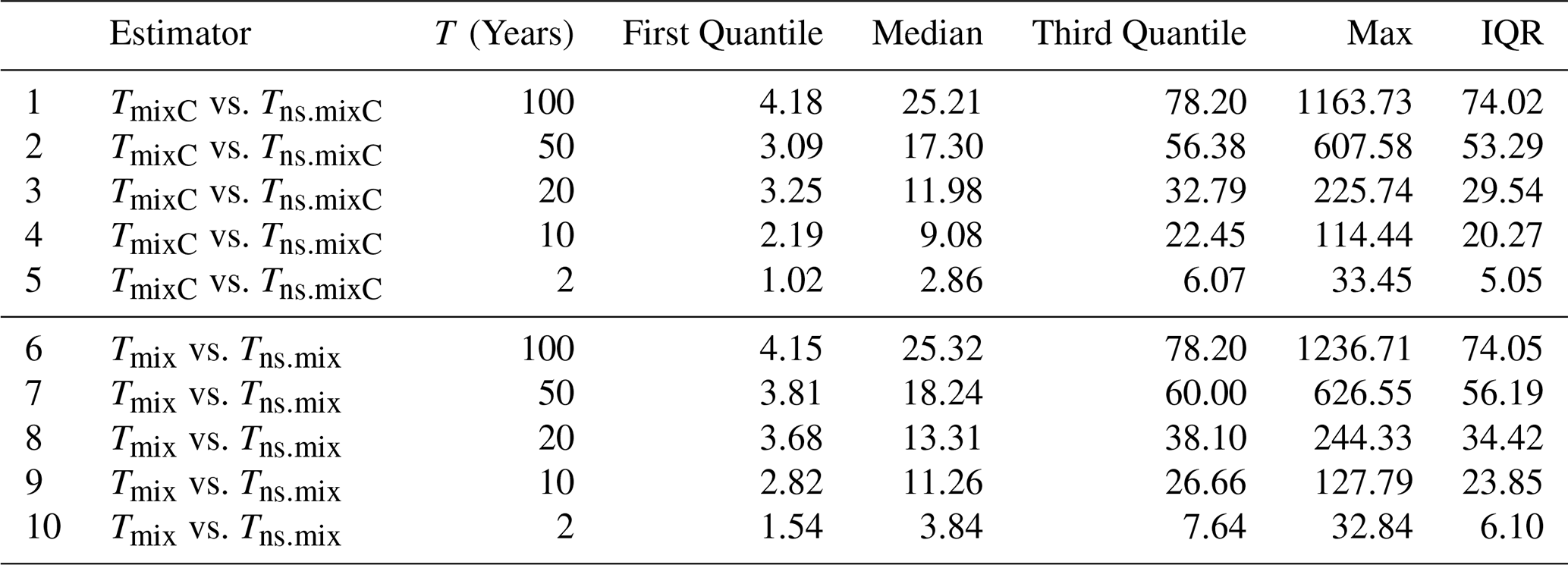
Building on the stationary comparison, we conduct three assessments to quantify the impact of non-stationarity modelling on low-flow return-period estimates. First, for catchments with evident non-stationarity, we compare return-period estimates for the beginning (1976) and end (2020) of the observation period. The resulting relative absolute deviations are summarised across catchments, and are reported in Table 1, thereby quantifying the temporal shift captured by the non-stationary framework. A clear pattern emerges: the deviations are largest for high return periods and decrease steadily towards more frequent events. For T=100 years, the median relative absolute deviation is 41.73 % for T_ns.mixC and 41.99 % for T_ns.mix, while for T=50 years the medians remain high at 32.72 % and 34.71 %, respectively. Even at T=10 years, the median deviations still reach about 20 %–26 %, and at T=2 years they remain close to 9 %–12 %. This indicates that between 1976 and 2020, the estimated return periods of low-flow events changed markedly in catchments with evident non-stationarity, particularly for rare events. It also implies that low-flow events classified as very rare in 1976, may have very different recurrence characteristics by 2020. The largest changes occur in the upper tail of the distribution, indicating that temporal change affects the severity assessment of extreme low-flow events more strongly than that of frequent events. Depending on the direction of change, a low-flow event of fixed magnitude may therefore have become either more frequent or less frequent by 2020.

Table 1 Summary statistics of the relative absolute deviation (%) of the non-stationary mixture-based estimators T_ns.mixC and T_ns.mix between the beginning and end of the observation period for catchments with evident non-stationarity.

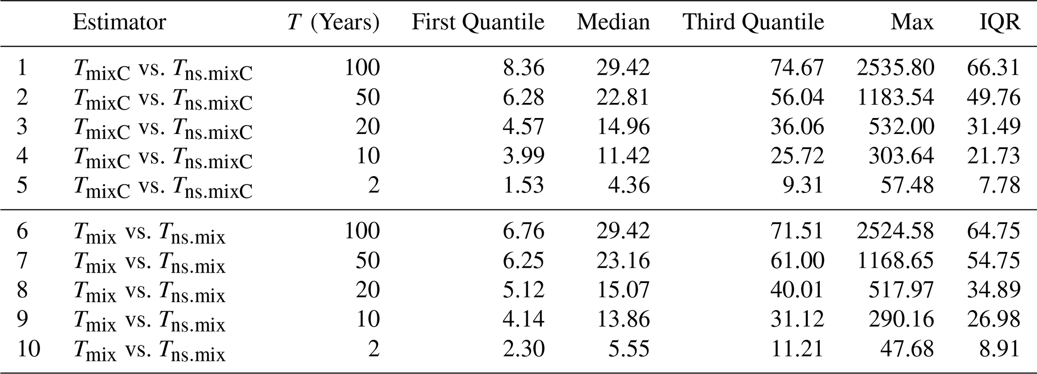
By comparison, Table 2 provides a practical measure of how far a stationary model can depart from a non-stationary formulation under recent conditions in catchments with evident non-stationarity. While this does not establish the error in an absolute sense, it does quantify the discrepancy incurred when temporal change is ignored. The same overall pattern is observed, with the largest deviations again occurring for high return periods and smaller deviations for more frequent events. For T=100 years, the median relative absolute deviation is 29.42 % for both estimator pairs, while for T=50 years it remains around 23 %. At lower return periods, the differences decrease further, but remain non-negligible, reaching about 11 %–14 % for T=10 years and 4 %–6 % for T=2 years. In practical terms, this means that, in catchments where non-stationarity is evident, stationary estimates may differ by around 30 % or more from non-stationary estimates for rare events. Compared with the previous assessment, these deviations are systematically smaller, as the earlier comparison captures the full temporal shift between 1976 and 2020 within the non-stationary framework, whereas the present one contrasts a fixed stationary estimate with the non-stationary estimate at a single point in time. Accordingly, the former describes temporal evolution, while the latter indicates the potential bias from representing recent low-flow conditions with a stationary model.

Table 2 Summary statistics of the relative absolute deviation (%) between the stationary estimators T_mixC and T_mix and their non-stationary counterparts T_ns.mixC and T_ns.mix, evaluated at the end of the observation period for catchments with evident non-stationarity.

Compared with the subset of catchments showing evident non-stationarity, however, the deviations are systematically smaller once all catchments are included. As shown in Table G1 at T=100 years, for example, the median deviation decreases from 29.42 % to about 25.2 %, and the same reduction appears at all return periods. This is consistent with expectations, because the full sample also includes catchments where non-stationarity is weak (or not significant). Including those catchments naturally reduces the overall contrast between stationary and non-stationary formulations. As illustrated in Fig. 5, deviations between stationary and non-stationary estimates are generally small for frequent events (T=2 years), but become much larger and more widespread for rare events (T=100 years), both in catchments with evident non-stationarity (Fig. 5a–b) and across the full set of catchments (Fig. 5c–d). In that sense, the pan-European comparison provides a more conservative estimate of the average effect of non-stationarity modelling.

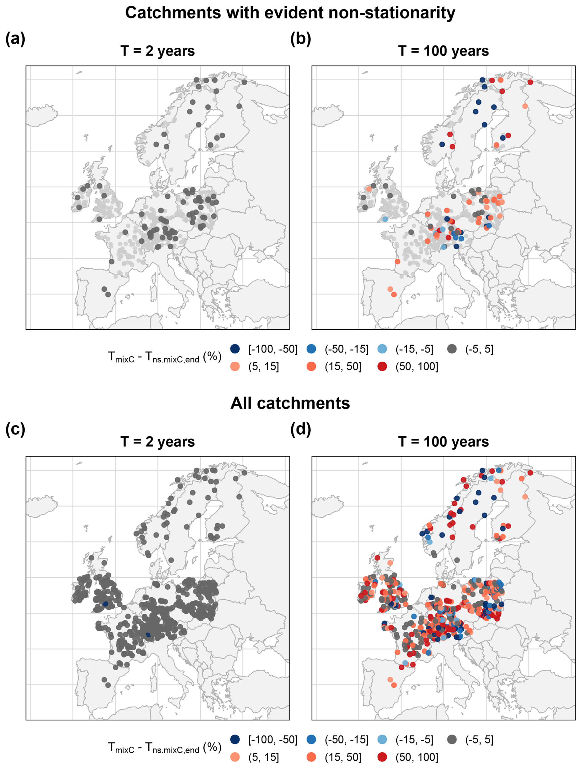
Figure 5 Spatial comparison of stationary and non-stationary return-period estimates across European catchments. Panels (a)–(b) show the relative deviation between T_mixC and the non-stationary end-of-period estimate $T_{\mathrm{ns}.\mathrm{mixC},\mathrm{end}}$ for catchments classified as non-stationary; panels (c)–(d) show the same comparison for all catchments.

Another notable result across all three comparisons is that the two mixture-based models remain very similar: The summary statistics for T_ns.mixC and T_ns.mix, as well as for the stationary versus non-stationary comparisons, differ only slightly. This suggests that the dominant effect arises from introducing temporal non-stationarity itself, rather than from the distinction between the mixture and mixture-copula formulations. In other words, once seasonal structure is already represented, the largest additional change arises from allowing the distribution parameters to vary with time and not by considering the dependency of events.

Overall, the results show that non-stationarity modelling has a tangible impact on low-flow frequency estimation, particularly for rare events. The largest deviations occur when the full temporal shift within the non-stationary framework is considered in catchments with evident non-stationarity, smaller but still substantial deviations arise when stationary and non-stationary formulations are compared under recent conditions in the same subset of catchments, and somewhat smaller deviations again are found when this comparison is extended to all catchments. This progression is physically plausible and suggests that the strongest benefits of non-stationary modelling are concentrated in catchments where temporal change is most evident, while the broader European data set still shows a meaningful overall effect.

5 Conclusions

This study developed and evaluated the non-stationary seasonal low-flow frequency analysis framework NSLFA_mixC, extending the stationary mixture and mixture-copula approaches to a non-stationary setting. The framework provides a consistent and unified way to represent seasonal low-flow behaviour, inter-seasonal dependence, and temporal change, and is particularly relevant where key assumptions of traditional low-flow frequency analysis are violated due to process heterogeneity and non-stationarity.

The results show that non-stationary behaviour is evident in in approximately 10 % of the near-natural European catchments used in this study, although its strength varies across regions and return periods. In the present application, non-stationarity is introduced through the location parameter, so temporal change is represented mainly as a shift in the lower bound of the seasonal low-flow distribution. Comparisons between the beginning and end of the observation period indicate that return period estimates can change significantly within the historical record, especially for rare events, implying that low-flow events considered very rare at the start of the record may have substantially different recurrence characteristics under recent conditions.

The comparison with stationary formulations further shows that ignoring non-stationarity can lead to substantial differences, particularly in catchments where temporal change is evident and especially for high return periods. At the same time, the non-stationary analysis confirms that the largest gain still comes from explicitly representing seasonal low-flow structure, while the additional refinement from the mixture copula-based approach is generally smaller. Overall, the results suggest a clear hierarchy of model gains: the largest improvement comes from accounting for seasonal process heterogeneity, followed by temporal non-stationarity, whereas the added gain from modelling inter-seasonal dependence is more modest. In this sense, NSLFA_mixC provides a coherent and flexible framework for describing historical changes in low-flow frequency behaviour across diverse European hydro-climatic settings.

5.1 Limitations and future work

Some limitations should be noted. In the present study, non-stationarity is introduced only through the location parameter. While this parsimonious formulation is attractive for interpretation and large-sample application, it may be insufficient since variability can also change over time. Moreover, the non-stationary model is used here solely to describe historical change and is not intended to predict future trends. A further challenge is that non-stationary models generally require sufficiently long data records to estimate temporal changes in a robust way. Where records are short, the additional parameters introduced by non-stationary formulations may be difficult to estimate, increase uncertainty and reduce the reliability of inferred trends. This is particularly relevant in low-flow applications, where data scarcity and limited record length remain common in many catchments.

These limitations point to several directions for future work. An important next step is to investigate whether temporal changes in low-flow variability can be represented parsimoniously as consequential changes associated with shifts in the mean, rather than by independently varying additional distribution parameters, while remaining consistent with the underlying physical processes driving change. Further work should also aim to more directly link the inferred temporal changes to physical drivers, such as temperature, precipitation deficits, snow processes, evaporative demand, catchment storage dynamics, and large-scale climate variability. It would also be useful to extend it to multivariate settings, such as low flow and high water temperature, which would be valuable given its relevance for aquatic ecosystem health. In addition, the present framework is developed using WEI3, supported by its theoretical basis for lower extremes and its established use in low-flow frequency analysis. Extending the framework to alternative marginal distributions would provide a useful assessment of its broader applicability. Finally, it would be useful to examine more explicitly how non-stationary low-flow frequency estimates can contribute to drought management, environmental flow assessment, and water-resources planning under changing climatic conditions.

Appendix A: Maximum-likelihood estimation

The parameters of the three-parameter Weibull (WEI3) distribution are estimated by maximum likelihood separately for the summer and winter low-flow series. Let $\mathit{\{}{q}_{\mathrm{t}}{\mathit{\}}}_{t=\mathrm{1}}^n$ denote a seasonal sample of low-flow minima.

In the stationary case, the location parameter μ is constant over time, and the log-likelihood function is given by

$$\begin{array}{}\text{(A1)}& \begin{array}{rl}& \mathrm{\ell }(\mathit{\xi },\mathit{\sigma },\mathit{\mu })=\sum _{t=\mathrm{1}}^n\\ & \left[\ln \left(\mathit{\xi }\right)-\ln \left(\mathit{\sigma }\right)+(\mathit{\xi }-\mathrm{1})\ln \left({\displaystyle \frac{q_{\mathrm{t}}-\mathit{\mu }}{\mathit{\sigma }}}\right)-{\left({\displaystyle \frac{q_{\mathrm{t}}-\mathit{\mu }}{\mathit{\sigma }}}\right)}^{\mathit{\xi }}\right],\end{array}\end{array}$$

defined for q_t>μ, with σ>0 and ξ>0.

In the non-stationary case, temporal variation in low-flow behaviour is introduced through a time-dependent location parameter,

$$\begin{array}{}\text{(A2)}& \mathit{\mu }\left(t\right)={\mathit{\beta }}_{\mathrm{0}}+{\mathit{\beta }}_{\mathrm{1}}t,\end{array}$$

while the scale and shape parameters are assumed constant. The corresponding log-likelihood function becomes

$$\begin{array}{}\text{(A3)}& \begin{array}{rl}& \mathrm{\ell }(\mathit{\xi },\mathit{\sigma },{\mathit{\beta }}_{\mathrm{0}},{\mathit{\beta }}_{\mathrm{1}})=\sum _{t=\mathrm{1}}^n\\ & \left[\ln \left(\mathit{\xi }\right)-\ln \left(\mathit{\sigma }\right)+(\mathit{\xi }-\mathrm{1})\ln \left({\displaystyle \frac{q_{\mathrm{t}}-\mathit{\mu }\left(t\right)}{\mathit{\sigma }}}\right)-{\left({\displaystyle \frac{q_{\mathrm{t}}-\mathit{\mu }\left(t\right)}{\mathit{\sigma }}}\right)}^{\mathit{\xi }}\right],\end{array}\end{array}$$

with q_t>μ(t) for all t.

In both cases, parameter estimation is carried out by minimising the negative log-likelihood subject to the constraints σ>0, ξ>0, and valid support of the distribution.

Appendix B: Sensitivity analysis of the seasonal low flow classification

Table B1 Sensitivity of the low-flow seasonality classification to the silhouette-width threshold used to identify catchments with mixed seasonality. The baseline threshold is s<0.20. Agreement refers to the percentage of catchments retaining the same classification as under the baseline threshold.

Table B2 Sensitivity of the physical interpretation of the PAM clusters to the seasonal definition. The baseline defines summer as April–October and winter as November–March.

Appendix C: Low flow regime classification with Mixture rate

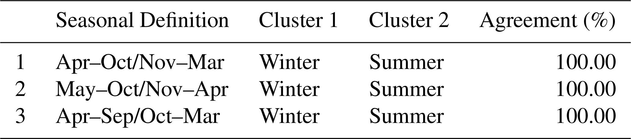
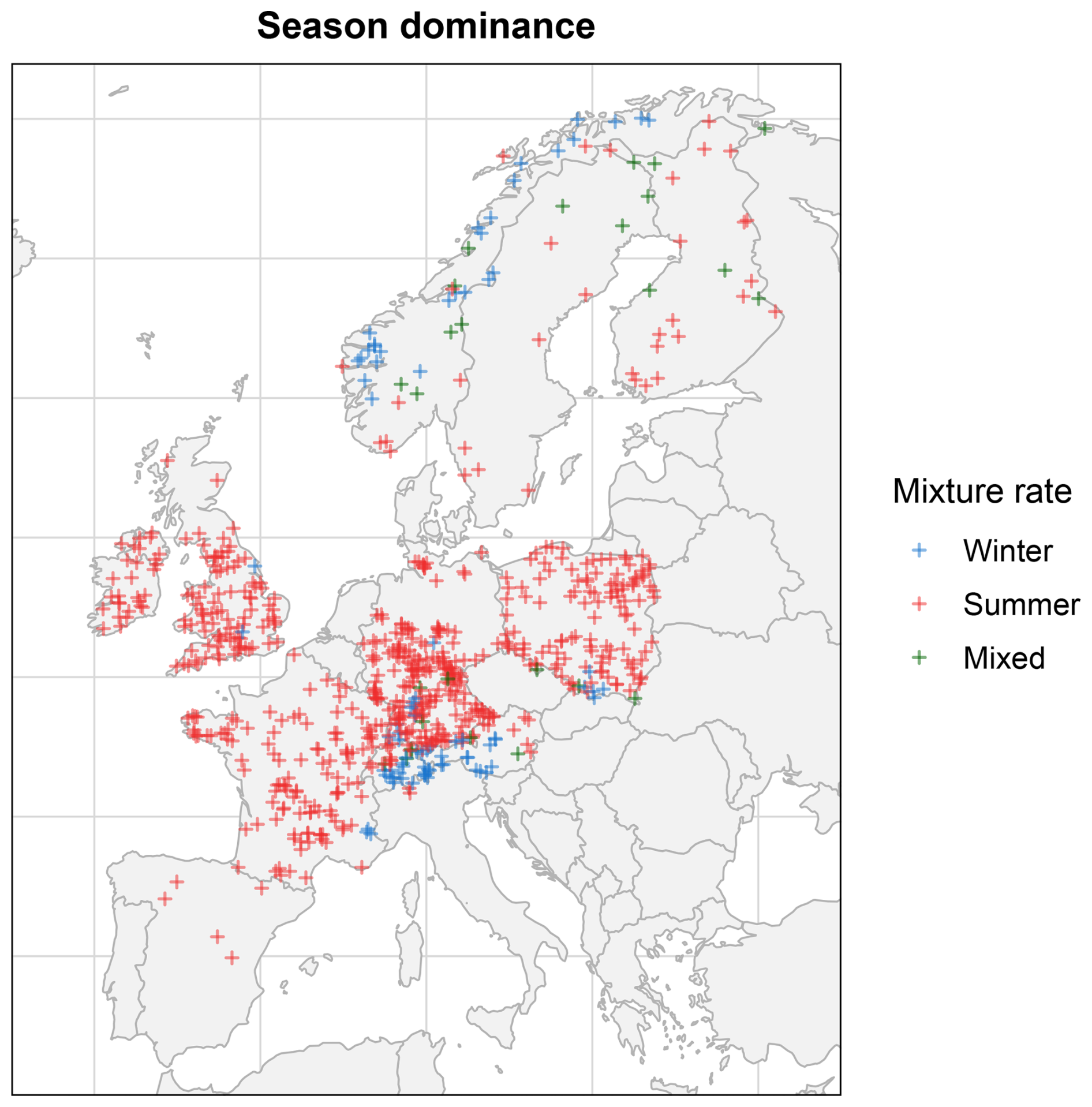
Figure C1 Spatial distribution of the dominant seasonal low-flow regime across the study catchments based on the mixture rate.

Appendix D: Spatial and hydrological characteristics of WEI3 fitting outcomes

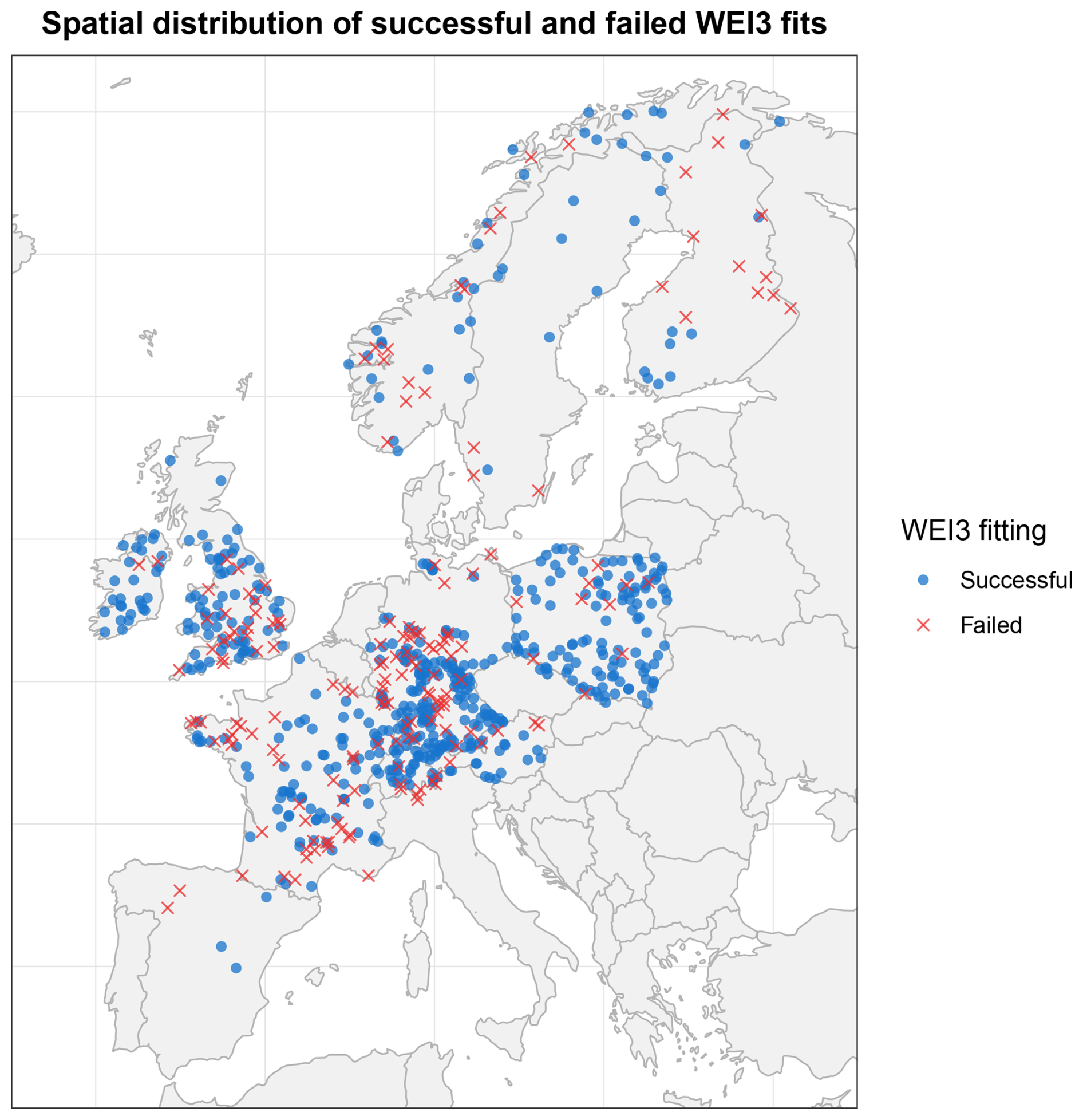
Figure D1 Spatial distribution of catchments with successful and unsuccessful WEI3 fits with MLE across the European study domain.

Table D1 Comparison of catchment characteristics, low-flow characteristics and distributional shape between catchments with successful and unsuccessful WEI3 fits. Values are reported as median [Q1–Q3]. Low-flow values are normalized by catchment area. p-values are based on Wilcoxon rank-sum tests.

Appendix E: Contrasting catchment example: Oksfjordvatn, Norway

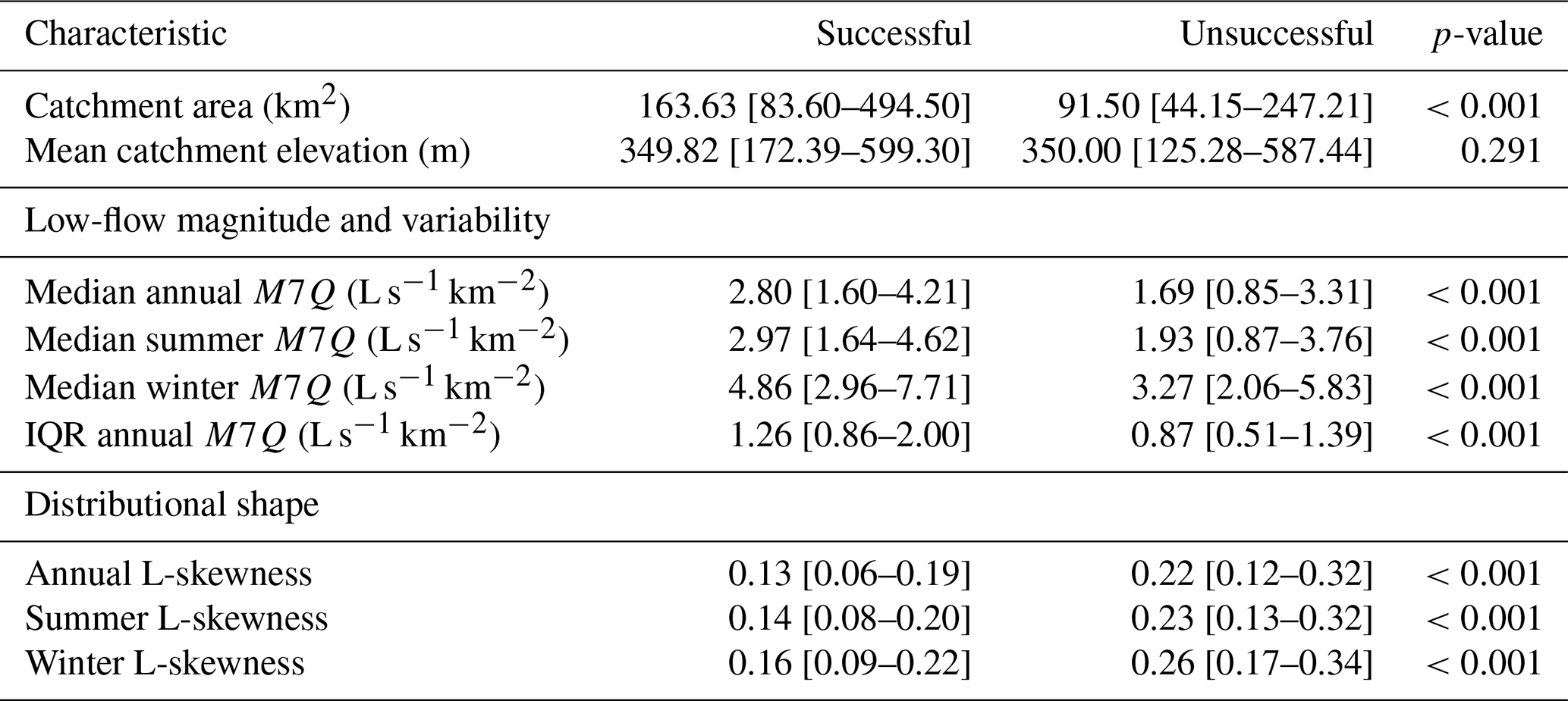
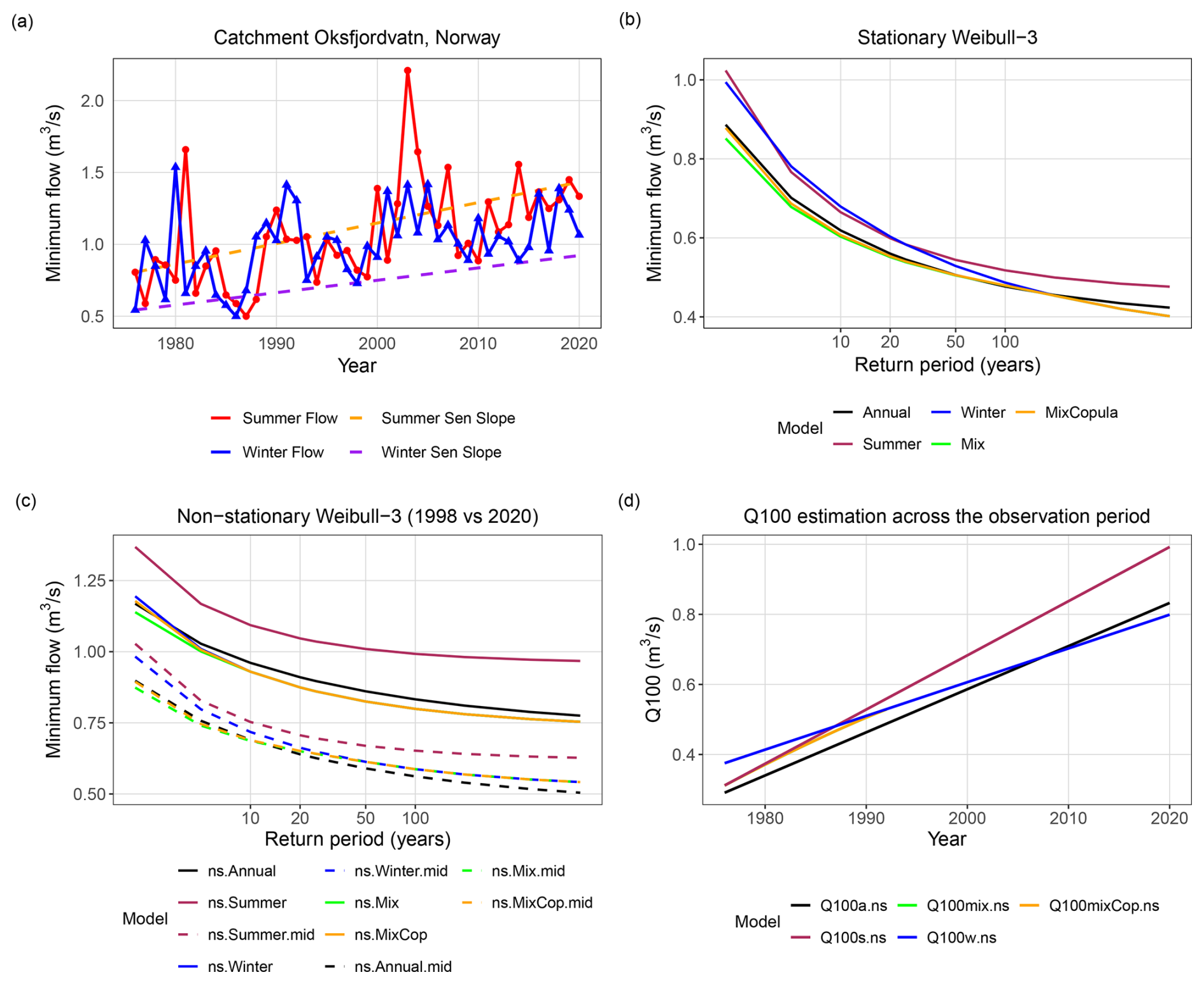
Figure E1 Application of the NSLFA_mixC framework to Oksfjordvatn, Norway. (a) Observed summer and winter minimum flows with corresponding Sen's slope trends. (b) Stationary WEI3 low-flow frequency estimates for the annual, summer, winter, mixture, and mixture-copula models. (c) Non-stationary low-flow frequency estimates evaluated at the midpoint (1998) and end (2020) of the observation period. (d) Temporal evolution of the estimated 100-year low-flow quantile (Q₁₀₀) over the observation period.

Appendix F: Performance gains of the stationary modelling

The stationary benchmark comparison confirms the findings of Laaha (2023b), with the main added value of the present analysis being the use of an extended and more recent observation period. As shown in Table F1, both mixture-based estimators deviate from the annual estimator, especially at high return periods (T=100), while the differences decrease toward more frequent events (T=2) as also illustrated in Fig.F1a–b. These findings support the conclusion that a conventional annual distribution may not adequately capture the combined influence of distinct summer and winter low-flow generating processes. In addition, Table F2 further shows that differences between T_mix and T_mixC are generally small for the most extreme events in most catchments, suggesting that seasonal dependence has only a minor influence in the distribution tail. For more frequent events, however, the deviations become more pronounced, indicating that dependence plays a more visible role outside the most extreme conditions.

Table F1 Summary statistics of the relative absolute deviation (%) of the stationary mixture-based estimators T_mixC and T_mix from the conventional annual estimator T.

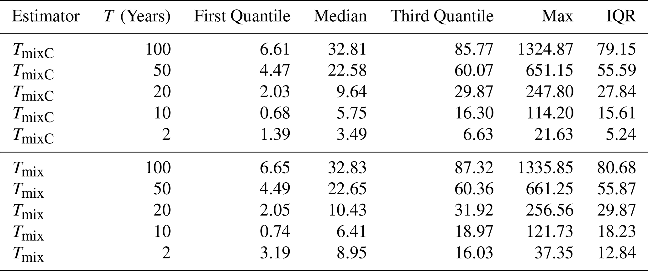
Table F2 Summary statistics of relative deviation of Δrd between the mix and the mix copula estimator (in %).

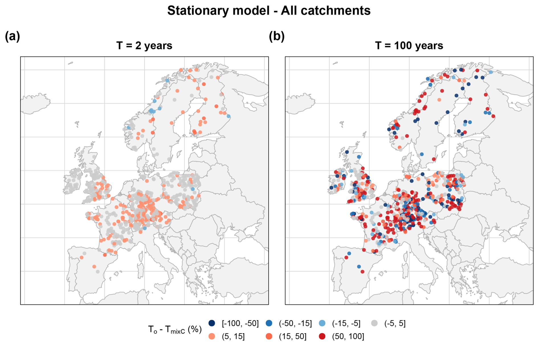
Figure F1 Spatial comparison of stationary models return-period estimates across European catchments. (a, b) show the relative deviation between the annual estimate T and the stationary mixed distribution-copula estimate T_mixC for return periods of 2 and 100 years.

Appendix G: Model gain between stationary and non-stationary estimators for all catchments

Table G1 Summary statistics of the relative absolute deviation (%) between the stationary estimators T_mixC and T_mix and their non-stationary counterparts T_ns.mixC and T_ns.mix, evaluated at the end of the observation period for all catchments.